Pressure Metrics and Manhattan Curves for Teichmüller Spaces of Punctured Surfaces

Abstract.

In this paper, we extend the construction of pressure metrics to Teichmüller spaces of surfaces with punctures. This construction recovers Thurston’s Riemannian metric on Teichmüller spaces. Moreover, we prove the real analyticity and convexity of Manhattan curves of finite area type-preserving Fuchsian representations, and thus we obtain several related entropy rigidity results. Lastly, relating the two topics mentioned above, we show that one can derive the pressure metric by varying Manhattan curves.

1. Introduction

Let $S=S_{g,n}$ be an orientable surface of genus $g$ and $n$ punctures with negative Euler characteristic. In this paper, we discuss how one can characterize Fuchsian representations and the geometry of ${\mathcal{T}}(S)$ the Teichmüller space of $S$ by studying dynamics objects associated with them. For example, we prove rigidity results via examining the shape of Manhattan curves, and we construct a Riemannian metric on ${\mathcal{T}}(S)$ by derivatives of pressure.

When $S$ has no puncture, results in this work are not new. Manhattan curves and rigidity results are, for instance, discussed in [Bur93, Sha98], and the pressure metric on ${\mathcal{T}}(S)$ is discovered in [McM08] and further investigated in [PS16, BCS18]. Nevertheless, when $S$ has punctures, especially when Fuchsian representations are not convex co-compact, much less results along this line are proved. Indeed, in such cases, their dynamics are much more complicated because the presence of parabolic elements.

Using a similar idea in [LS08, Kao18], we study geodesics flows over hyperbolic surfaces with cusps by countable state Markov shifts and corresponding suspension flows. Notice that for countable state Markov shifts, different from compact cases, for unbounded potentials without sufficient control of their regularity and values around cusps, the pressure of their perturbation might not only lose the analyticity but also information of some thermodynamics data. For example, time changes for suspension flows over a non-compact Markov shift may not take equilibrium states to equilibrium states for some potentials (cf. [CI18]).

To overcome these issues, we carefully study the associated geometric potential (or the roof function of the suspension flow). By doing so, we know exactly where the pressure function (of geometric potentials and their weighted sums) is analytic. Thus, we can mimic the procedure used in compact cases. More precisely, we derive a version of Bowen’s formula which relating the topological entropy of the geodesic flow and the corresponding roof function. With Bowen’s formula and the analyticity of pressure, we prove the convexity of Manhattan curves, and using the second derivative of pressure we construct a Riemannian metric on ${\mathcal{T}}(S)$.

To put our results in context, we now introduce necessary notations and definitions. Recall that a representation $\rho\in{\rm Hom}(\pi_{1}S,\mathrm{PSL}(2,\mathbb{R}))$ is Fuchsian if it is discrete and faithful, and $\rho$ has finite area if the hyperbolic surface $X_{\rho}=\rho(\pi_{1}S)\backslash\mathbb{H}$ has finite area. We say two finite area Fuchsian representations $\rho_{1},\rho_{2}$ are type-preserving if there exists an isomorphism $\iota:\rho_{1}(\pi_{1}S)\to\rho_{2}(\pi_{1}S)$ sending parabolic elements to parabolic elements and hyperbolic elements to hyperbolic elements. Here ${\rm PSL}(2,\mathbb{R})$ refers to the space of orientation preserving isometries of the hyperbolic plane $\mathbb{H}$.

Let $\rho_{1}$ and $\rho_{2}$ be two Fuchsian representations. Recall that $d_{\rho_{1},\rho_{2}}^{a,b}$ the weighted Manhattan metric on $\mathbb{H}\times\mathbb{H}$ with respect to $\rho_{1},\rho_{2}$ is given by, fixing $o=(o_{1},o_{2})$, $d_{\rho_{1},\rho_{2}}^{a,b}(o,\gamma o):=ad(o_{1},\rho_{1}(\gamma)o_{1})+bd(o_{2},\rho_{1}(\gamma)o_{2})$ for $\gamma\in\pi_{1}(S)$ where $d$ is the hyperbolic distance on $\mathbb{H}$. Notice that we only interested in non-negative weights, i.e., $a,b\geq 0$ and $ab\neq 0$. We denote the associated Poincaré series by

$$Q_{\rho_{1},\rho_{2}}^{a,b}(s):={\displaystyle\sum_{\gamma\in\pi_{1}(S)}e^{-s\cdot d_{\rho_{1},\rho_{2}}^{a,b}(o,\gamma o)}.}$$

Definition 1.1 (Manhattan Curve).

The Manhattan curve ${\mathcal{C}}(\rho_{1},\rho_{2})$ of $\rho_{1}$, $\rho_{2}$ is given by

$${\mathcal{C}}(\rho_{1},\rho_{2}):=\{(a,b)\in\mathbb{R}_{\geq 0}\times\mathbb{R}_{\geq 0}\backslash(0,0):\ \delta_{\rho_{1},\rho_{2}}^{a,b}=1\}$$

where $\delta_{\rho_{1},\rho_{2}}^{a,b}$ is the critical exponent of $Q_{\rho_{1},\rho_{2}}^{a,b}(s)$, i.e., $Q_{\rho_{1},\rho_{2}}^{a,b}(s)$ is divergent if $s<\delta_{\rho_{1},\rho_{2}}^{a,b}$ and is convergent if $s>\delta_{\rho_{1},\rho_{2}}^{a,b}$.

By definition, one can regard ${\mathcal{C}}(\rho_{1},\rho_{2})$ as a generalization of the critical exponents for $\rho_{1}$ and $\rho_{2}$. Obviously, taking $a=0$ (respectively, $b=0$), $\delta_{\rho_{1},\rho_{2}}^{a,b}$ reduces to $\delta_{\rho_{1}}$ the classical critical exponent for $\rho_{1}$ (respectively, $\delta_{\rho_{2}}$). By Otal and Peigné [OP04], we know $\delta_{\rho_{1}}$ is also the topological entropy of the geodesic flow over $X_{\rho_{1}}$.

As mentioned above, using a symbolic model given in [LS08], for every finite area Fuchsian representation $\rho$, we can code the geodesic flow over $X_{\rho}$. Elaborated discussion of the coding of geodesic flows is in Section 3. We briefly introduce the idea and strategy below. We will associate the geodesic flow on the smaller special section $\Omega_{0}\subset T^{1}X_{\rho}$ with a suspension flow $(\Sigma^{+},\sigma,\tau_{\rho})$ where $(\Sigma^{+},\sigma)$ is a countable state Markov shift and $\tau_{\rho}:\Sigma^{+}\to\mathbb{R}^{+}$ is the roof function. Furthermore, by the construction, the roof function $\tau_{\rho}$ is a continuous function prescribing the length of closed geodesics. We sometimes call $\tau_{\rho}$ the geometric potential of $\rho$. Moreover, one important feature of this symbolic model is that if $\rho_{1},\rho_{2}$ are finite area type-preserving Fuchsian representations, then they correspond to the same Markov shift $(\Sigma^{+},\sigma)$ but to different roof functions $\tau_{\rho_{1}},\tau_{\rho_{2}}$. In other words, we can use roof functions to characterize finite area type-preserving Fuchsian representations.

Using this symbolic model, we can characterize ${\mathcal{C}}(\rho_{1},\rho_{2})$ as solutions of a version of Bowen’s formula. Furthermore, we derive the first main result of the paper:

Theorem A.

Let $\rho_{1}$, $\rho_{2}$ be two finite area type-preserving Fuchsian representations. Then ${\mathcal{C}}(\rho_{1},\rho_{2})$ is a real analytic curve, and ${\mathcal{C}}(\rho_{1},\rho_{2})$ is strictly convex unless $\rho_{1}$ and $\rho_{2}$ are conjugate in ${\rm PSL}(2,\mathbb{R})$, in such cases ${\mathcal{C}}(\rho_{1},\rho_{2})$ is a straight line.

Using the shape of Manhattan curve, we can further prove rigidity results related with following dynamics quantities.

Definition 1.2.

Let $\rho_{1}$, $\rho_{2}$ be a pair of Fuchsian representations.

1. Bishop-Steiger entropy $h_{BS}(\rho_{1},\rho_{2})$ of $\rho_{1}$ and $\rho_{2}$ is defined as

   $$h_{{\rm BS}}(\rho_{1},\rho_{2}):={\displaystyle\lim_{T\to\infty}\frac{1}{T}\ln\left(\#\{[\gamma]\in[\pi_{1}(S)]:d(o,\rho_{1}(o,\gamma o))+d(o,\rho_{2}(o,\gamma o))\leq T\}\right)}.$$

2. The intersection number ${\rm I}(\rho_{1},\rho_{2})$ of $\rho_{1}$ and $\rho_{2}$ is defined as

   $${\rm I}(\rho_{1},\rho_{2}):=\lim_{n\to\infty}\frac{l_{2}[\gamma_{n}]}{l_{1}[\gamma_{n}]}$$

   where $\{[\gamma_{n}]\}_{n=1}^{\infty}$ is a sequence of conjugacy classes for which the associated closed geodesics $\gamma_{n}$ become equidistributed on $X_{\rho_{1}}$ with respect to area.

Using a dynamics interpretation of ${\rm I}(\rho_{1},\rho_{2})$ and the convexity and analyticity of pressure, we recover the following results of Bishop and Steiger [BS93], and Thurston.

Theorem B.

Let $\rho_{1}$, $\rho_{2}$ be a pair of area type-preserving Fuchsian representations, we have

1. $($Bishop-Steiger Rigidity$)$ $h_{{\rm BS}}(\rho_{1},\rho_{2})\leq\frac{1}{2}$, and the equality holds if and only if $\rho_{1}$ and $\rho_{2}$ are conjugate in $\mathrm{PSL}(2,\mathbb{R})$.

2. $($The Intersection Number Rigidity$)$ ${\rm I}(\rho_{1},\rho_{2})\geq 1$, and the equality holds if and only if $\rho_{1}$ and $\rho_{2}$ are conjugate in $\mathrm{PSL}(2,\mathbb{R})$.

Remark 1.3.

1. One might prove ${\mathcal{C}}(\rho_{1},\rho_{2})$ is $C^{1}$ and Theorem B without employing symbolic dynamics. Nevertheless, symbolic dynamics provides a convenient approach to control the analyticity of pressure, and hence to prove the analyticity of ${\mathcal{C}}(\rho_{1},\rho_{2})$.

2. It is no very clear why ${\rm I}(\rho_{1},\rho_{2})$ is well-defined. We will justify it in Section 3.

3. The intersection number rigidity is known as a work of Thurston amount experts. However, due to the limited knowledge of the author, for the non-convex co-compact cases we cannot find a reference of it.

We now change gear from pairs of Fuchsian representations to the space of conjugacy classes of Fuchsian representations, that is, the Teichmüller space of $S=S_{g,n}$. Recall that the Teichmüller space of $S$ is defined as

$${\mathcal{T}}(S):={\rm Hom_{tp}^{F}}(\pi_{1}(S),\mathrm{PSL}(2,\mathbb{R}))/\sim$$

where ${\rm Hom_{tp}^{F}}(\pi_{1}(S),\mathrm{PSL}(2,\mathbb{R}))$ is the space of finite area type-preserving Fuchsian representations, and $\rho_{1}\sim\rho_{2}$ if they are conjugate in $\mathrm{PSL}(2,\mathbb{R})$.

Through the symbolic model, there is a thermodynamic mapping $\Psi:{\mathcal{T}}(S)\to{\rm\mathbf{P}}$ where ${\rm\mathbf{P}}$ is a special space of continuous functions over $\Sigma^{+}$ containing geometric potentials. Using the pressure and variance we can define a norm $||\cdot||_{{\rm P}}$ over ${\rm\mathbf{P}}$. Using the pullback of $||\cdot||_{{\rm P}}$, we can define a Riemannian metric $||\cdot||$ on ${\mathcal{T}}(S)$. We call this Riemannian metric the pressure metric. Moreover, $||\cdot||$ can also be derived by the Hessian of the intersection number:

Theorem C (The Pressure Metric).

Suppose $\rho_{t}\in{\mathcal{T}}(S)$ is an analytic path for $t\in(-\varepsilon,\varepsilon)$. Then ${\rm I}(\rho_{0},\rho_{t})$ is real analytic and

$$||\dot{\rho}_{0}||^{2}:=||{\rm d}\psi(\dot{\rho}_{0})||_{{\rm P}}^{2}=\left.\frac{{\rm d}^{2}{\rm I}(\rho_{0},\rho_{t})}{{\rm d}t^{2}}\right|_{t=0}$$

defines a Riemannian metric on ${\mathcal{T}}(S_{g,n})$.

We briefly discuss the history of this Riemannian metric $||\cdot||$ on ${\mathcal{T}}(S_{g,n})$. When $n=0$, Thurston first discovered it by using the Hessian of the intersection number. Thus, this Riemannian metric is also known as Thurston’s Riemannian metric. Moreover, proved by Wolpert [Wol86], this Riemannian metric is exactly the Weil-Petersson metric on ${\mathcal{T}}(S_{g,0})$. McMullen [McM08] recovered this Riemannian metric using thermodynamic formalism and called it the pressure metric. Carrying over the same spirit, Bridgeman, Canary, Labourie, and Sambarino [BCLS15] generalized this dynamics approach and constructed a Riemannian metric on the space of Anosov representations, i.e., a higher rank generalization of ${\mathcal{T}}(S_{g,0})$. Our Theorem C extends the pressure metric and Thurston’s construction to ${\mathcal{T}}(S_{g,n})$ for $n>0$.

The last result of the paper is to link the two main topics in this work: Manhattan curves and the pressure metric. We prove that when we look at a path in ${\mathcal{T}}(S)$, the variation of corresponding Manhattan curves contains information of the pressure metric. Similar result has been proved by Pollicott and Sharp [PS16] when $S$ is a closed surface. We generalize it to surfaces with punctures.

Theorem D.

Let $(s,\chi_{t}(s))$ be the coordinates of points on the Manhattan curve ${\mathcal{C}}(\rho_{0},\rho_{t})$, then we have

$$\left.\frac{{\rm d}^{2}{\mathcal{\chi}}_{t}(s)}{{\rm d}t^{2}}\right|_{t=0}=s(s-1)\cdot||\dot{\rho}_{0}||^{2}\ \ {\rm for\ }s\in(0,1).$$

The paper is organized as follows. In Section 2, we introduce some background knowledge of geometry and thermodynamic formalism of countable state Markov shifts. In Section 3 we discuss the coding of geodesic flows and important properties of the corresponding roof functions. We study the analyticity of the pressure function in Section 4. Section 5 is devoted to investigating the shape of Manhattan curve and rigidity. In Section 6, we construct the pressure metric. In the last section, we focus on the relation between Manhattan curves and the pressure metric.

Acknowledgement.

The author is grateful to Prof. François Ledrappier for proposing the problem and numerous supports, to Prof. Dick Canary for many insightful suggestions and helps. Substantial portions of this paper were written while the author was visiting Prof. Jih-Hsin Cheng at Academia Sinica, Taiwan. The author would like to thank Prof. Jih-Hsin Cheng and Academia Sinica for their hospitality. The author is partially supported by the National Science Foundation Postdoctoral Research Fellowship under grant DMS 1703554.

2. Preliminary

2.1. Geometry

Through out this paper, $S=S_{g,n}$ is an orientable surface of $g$ genus and $n$ punctures and with negative Euler characteristic. In this work, we are interested in finite area hyperbolic surfaces homemorphic to $S$, that is, $S$ pair with a Riemannian metric ${\rm g}$ of Gaussian curvature -1. Notice that every such surface $(S,{\rm g)}$ can be obtained by a Fuchsian representation. More precisely, $(S,{\rm g)}$ is isomorphic to the hyperbolic surface $X_{\rho}=\rho(\pi_{1}(S))\backslash\mathbb{H}$.

For short, let us denote $\rho(\pi_{1}S)$ by $\Gamma$. Recall that $\partial_{\infty}\mathbb{H}$ the boundary of $\mathbb{H}$ is defined as $\mathbb{R}\cup\{0\}$, and $\Lambda(\Gamma):=\overline{\{\gamma\cdot o:\gamma\in\Gamma\}}$ denotes the limit set of $\Gamma$. An element $\gamma\in\Gamma$ is called hyperbolic if $\gamma$ has two fixed points on $\Lambda(\Gamma)$, namely, the attracting fixed point $\gamma_{+}$ (i.e., $\lim_{n\to\infty}\gamma^{n}o=\gamma_{+}$) and the repelling fixed point $\gamma_{-}$ (i.e., $\lim_{n\to-\infty}\gamma^{n}o=\gamma_{-}$); $\gamma$ is called parabolic if it has one fixed point. Because $X_{\rho}$ is negatively curved, we know that every closed geodesic $\lambda$ on $X_{\rho}$ corresponds to a unique hyperbolic element $\gamma$ (up to conjugation), and vice versa. Moreover, the length of $\lambda$ equals to $l[\gamma]$ the translation distance of $\gamma$, that is, $l[\gamma]:=\min\{d(x,\gamma x):x\in\mathbb{H}\}$.

A natural dynamical system associated to $X_{\rho}$ is the geodesic flow $g_{t}:T^{1}X_{\rho}\to T^{1}X_{\rho}$ on the unit tangent bundle $T^{1}X_{\rho}$, which translates many geometric problems to dynamics problems. We recall that the Busemann function $B:\partial_{\infty}\mathbb{H}\times\mathbb{H}\times\mathbb{H}$ is defined as

$$B_{\xi}(x,y):={\displaystyle\lim_{z\to\xi}d(x,z)-d(y,z)}$$

for $x,y,z\in\mathbb{H}$ and $\xi\in\partial_{\infty}\mathbb{H}.$ Lift the geodesic flow $g_{t}:T^{1}X_{\rho}\to T^{1}X_{\rho}$ to its universal covering $T^{1}\mathbb{H}$, by abusing the notation, we have the geodesic flow $g_{t}:T^{1}\mathbb{H}\to T^{1}\mathbb{H}.$

Recall that two Fuchsian representations $\rho_{1}$, $\rho_{2}$ are type-preserving if there exists an isomorphism $\iota:\rho_{1}(\pi_{1}S)\to\rho_{2}(\pi_{1}S)$ such that $\iota$ sends hyperbolic elements to hyperbolic elements and parabolic elements to parabolic elements. The following theorem indicates that if $\rho_{1},\rho_{2}$ are type-preserving finite area Fuchsian representations, then we can link $X_{\rho_{1}}$ and $X_{\rho_{2}}$ is a controlled manner.

Theorem 2.1 (Fenchel-Nielsen Isomorphism Theorem; [Kap09], Theorem 5.5, 8.16, 8.29).

Suppose $\rho_{1},\rho_{2}$ are two finite area type-preserving Fuchsian representations of $\pi_{1}S$. Then there exists an bilipschitz homeomorphism ${\rm b}:X_{\rho_{1}}\to X_{\rho_{2}}$. Moreover, one can extend ${\rm b}$ to an equivarient bilipschitz map, abusing the notation, ${\rm b}:\partial_{\infty}\mathbb{H}\cup\mathbb{H}\to\partial_{\infty}\mathbb{H}\cup\mathbb{H}$.

Remark 2.2.

In [Kap09], the homeomorphism ${\rm b}:X_{\rho_{1}}\to X_{\rho_{2}}$ is stated to be quasiconformal. Nevertheless, using Mori’s Theorem (cf. p.30 [Ahl06]) it is not hard to see that quasiconformal homeomorphisms are indeed bilipschitz maps.

In the following, we state a special case of [Kim01, Theorem A].

Theorem 2.3 (Marked Length Spectrum Rigidity).

Let $\rho_{1},\rho_{2}:\pi_{1}(S)\to{\rm PSL}(2,\mathbb{R})$ be Zariski dense Fuchsian representations. Suppose $\rho_{1},\rho_{2}$ have the same marked length spectrum, that is, $l[\rho_{1}(\gamma)]=k\cdot l[\rho_{2}(\gamma)]$ for some $k>0$ and for sufficiently many yet finite $\gamma\in\pi_{1}(S)$. Then $\rho_{1}$ and $\rho_{2}$ are conjugate in ${\rm PSL}(2,\mathbb{R})$.

Remark 2.4.

1. A representation $\rho:\pi_{1}(S)\to{\rm PSL}(2,\mathbb{R})$ is called Zariski dense if it is irreducible and $\rho(\pi_{1}(S))$ has no global fixed point on $\partial_{\infty}\mathbb{H}$. It is clear that finite area Fuchsian representations are Zariski dense.

2. The above result should be known before Kim, and [Kim01, Theorem A] is much more general than the above one. Nevertheless for the convenience we quote [Kim01, Theorem A].

2.2. Countable State Markov Shifts

In this subsection we aim to introduce terminologies of thermodynamic formalism for countable state (topological) Markov shifts. Reader can find more details in Mauldin’s and Urbański’s book [MU03] and Sarig’s note [Sar09].

Let ${\mathcal{A}}$ a countable set and $\mathbb{A}=(t_{ij})_{{\mathcal{A}}\times{\mathcal{A}}}$ be a matrix of zeros and ones with no columns or rows are all zeros.

Definition 2.5 (Countable State Markov Shift).

The (one-sided) countable state Markov shift with set of alphabet (or states) ${\mathcal{\mathcal{A}}}$ and transition matrix $\mathbb{A}$ is defined by

$$\Sigma^{+}_{\mathbb{A}}:=\{x=(x_{i})\in{\mathcal{A}}^{\mathbb{N}}:t_{x_{n}x_{n+1}}=1\ {\rm\forall}n\in\mathbb{N}\}$$

equipped with the topology generated by the collection of cylinders

$$[a_{0},...,a_{n}]:=\{x\in\Sigma^{+}_{\mathbb{A}}:x_{i}=a_{i},0\leq i\leq n\}\ \ (n\in\mathbb{N},a_{0},...,a_{n}\in{\mathcal{A}})$$

and coupled the the left (shift) map $\sigma:(x_{0},x_{1},x_{2}...)\mapsto(x_{1},x_{2},...)$.

A word of length $n$ on an alphabet $\mathcal{A}$ is a finite sequence $(a_{0},a_{1},...,a_{n-1})\in{\mathcal{A}}^{n-1}$ for all $n\in\mathbb{N}\backslash\{0\},$ and a word $(a_{0},a_{1},...,a_{n-1})$ is admissible with respect to $\mathbb{A}=(t_{ab})_{\mathcal{A}\times\mathcal{A}}$ if $t_{a_{i}a_{j}}=1$.

From now on we will omit the subscript $\mathbb{A}$ from $\Sigma^{+}_{\mathbb{A}}$ and simply use $\Sigma^{+}$ for one-sided Markov shifts because our discussion here only focus on a fixed transition matrix.

Recall that a Markov shift $(\Sigma^{+},\sigma)$ is topologically transitive if for all $a,b\in\mathcal{A}$ there exists an admissible word $(a,...,b)$, and is topological mixing if for all $a,b\in\mathcal{A}$ there exists a number $N_{ab}$ such that for all $n\geq N_{ab}$ there exists an admissible word $(a,...,b)$ of length $n$.

Let $g:\Sigma^{+}\to\mathbb{R}$ be a function. For $n\geq 1,$ the $n$-th variation of $g$ is defined by

$${\rm V}_{n}(g):=\sup\{|g(x)-g(y)|:\ x,y\in\Sigma^{+},x_{i}=y_{i}\ {\rm for\ }0\leq i\leq n-1\}.$$

When $\sum_{n=0}^{\infty}{\rm V}_{n}(g)<\infty$ we say that $g$ has summable variations, and in particular, we call $g$ a locally Hölder continuous function if there exists $C>0$ and $\theta\in(0,1)$ such that ${\rm V}_{n}(g)\leq C\cdot\theta^{n}$ for $n\geq 1.$

We remark that when the set of alphabet ${\mathcal{A}}$ is finite the Markov shift is called a subshift of finite type, and in that case $\Sigma^{+}$ is a compact set. When $\mathcal{A}$ is infinite $\Sigma^{+}$ is no longer compact. Nevertheless, countable state Markov shifts with the following property can be studied similarly as in the compact cases.

Definition 2.6 (BIP).

We say $(\Sigma^{+}_{\mathbb{A}},\sigma)$ has the big image and preimages (BIP) property if there exists a finite collection of states $s_{1},s_{2},...,s_{n}\in\mathcal{A}$ such that for every state $s\in\mathcal{A}$ there are some $i,j\in\{1,2,..,n\}$ such that $(s_{i},s)$, $(s,s_{j})$ are admissible.

Definition 2.7 (Topological Pressure for Countable State Markov Shifts).

Let $(\Sigma^{+},\sigma)$ be a topologically mixing Markov shifts and $g:\Sigma^{+}\to\mathbb{R}$ has summable variations. The topological pressure (or the Gurevich pressure) of $g$ is defined by

$$P(g):=\lim_{n\to\infty}\frac{1}{n}\log\sum_{x\in{\rm Fix}^{n}}e^{S_{n}g(x)}\mathds{1}{}_{[a]}(x),$$

where ${\rm Fix}^{n}:=\{x\in\Sigma^{+}:\sigma^{n}(x)=x\}$, $a\in\mathcal{A}$ is any state, and $S_{n}g(x)=g(x)+...+g(\sigma^{n-1}(x))$ is the $n$-th ergodic sum of $g$.

Notice that the topological pressure is independent on the state $a\in\mathcal{A}$ (cf. [Sar09]).

Theorem 2.8 (Variational Principle; [Sar99] Theorem 3).

Let $(\Sigma^{+},\sigma)$ be a topologically mixing Markov shifts and $g:\Sigma^{+}\to\mathbb{R}$ has summable variations. If $\sup g<\infty$ then

$$P(g)=\sup\{h_{\sigma}(m)+\int_{\Sigma^{+}}g\,\mathrm{d}m:\ m\in{\mathcal{M}_{\sigma}}\ {\rm and}\ -\int_{\Sigma^{+}}g\,\mathrm{d}m<\infty\}$$

where $h_{\sigma}(m)$ is the measure theoretic entropy of $m$ and ${\mathcal{M}}_{\sigma}$ is the set of $\sigma-$invariant Borel probability measures on $\Sigma^{+}$.

We want to remark that although Mauldin and Urbański, and Sarig defined countable state Markov shifts and the topological pressure differently. However, when the Markov shift is topologically mixing and has the BIP property, their definition are the same (cf. [MU01, Section 7]). Since in this paper we only focus on topologically mixing Markov shifts with the BIP property, we will use both results from Mauldin and Urbański, and Sarig.

Recall that a measure $m\in\mathcal{M_{\sigma}}$ is called an equilibrium state for $g$ if $P(g)=h_{\sigma}(m)+\int g\,\mathrm{d}m$. A measure $\nu\in{\mathcal{M}}_{\sigma}$ is called a Gibbs measure for $g$ if there exists constants $G>1$ and $P$ such that for all cylinder $[a_{0},...,a_{n-1}]$ and for very $x\in[a_{0},...,a_{n-1}]$ we have

$$\frac{1}{G}\leq\frac{\nu[a_{0},a_{1},...,a_{n-1}]}{\exp[S_{n}g(x)-nP]}\leq G.$$

Remark 2.9.

We would like to point out that there are subtle differences between Gibbs states and equilibrium states. Every equilibrium state is a Gibbs state but not vice versa. More precisely, if $g$ is locally Hölder with finite pressure and $\sup g<\infty$. Then $g$ has a unique Gibbs measure $\nu_{g}$, and $g$ has at most one equilibrium state. Furthermore, with the additional condition $-\int g\,\mathrm{d}\nu_{g}<\infty$, we know the unique Gibbs state $\nu_{g}$ is the equilibrium state for $g$ (cf. [Sar09, Theorem 4.5, 4.6, 4.9] and [MU03, Theorem 2.2.4, 2.2.9]).

Two functions $f,g:\Sigma^{+}\to\mathbb{R}$ are cohomologus, denoted by $f\sim g$, if there exists a function $h:\Sigma^{+}\to\mathbb{R}$ such that $f=g+h-h\circ\sigma$ where $h$ is called a transition function. The following theorem shows that the thermodynamic data are invariant in each cohomologus class of locally Hölder continuous functions.

Theorem 2.10.

[MU03, Theorem 2.2.7] Suppose $(\Sigma^{+},\sigma)$ is topologically mixing, and $f,g:\Sigma^{+}\to\mathbb{R}$ are locally Hölder continuous function with Gibbs measures $\nu_{f}$ and $\nu_{g}$, respectively. Then the following are equivalent:

1. $\nu_{f}=\nu_{g}$.

2. $($Livšic Theorem$)$ There exists a constant $R>0$ such that $\forall$ $n\geq 1$ and $x\in{\rm Fix}^{n}$ we have $S_{n}f(x)-S_{n}g(x)=nR$.

3. $f-g$ is cohomologus to a constant $R$ via a bounded Hölder continuous transition function.
   Moreover, when above assertions are true, then $R=P(f)-P(g)$.

We remark that we can define a two-sided countable state Markov shift $\Sigma_{\mathbb{A}}$ as

$$\Sigma_{\mathbb{A}}:=\{x=(x_{i})\in{\mathcal{A}}^{\mathbb{Z}}:t_{x_{n}x_{n+1}}=1\ {\rm\forall}n\in\mathbb{Z}\}$$

and define similarly all the thermodynamics data. Notice that if a potential on a two-sided shift space $(\Sigma,\sigma)$ is only depending on its future coordinate, then to understand the associated thermodynamics data, it is sufficient to study its behavior on the one-sided shift $(\Sigma^{+},\sigma)$. For a two-sided sequence $(...,a,\dot{b},c,...)$, $\dot{b}$ means $b$ is at the zero-th coordinate, i.e., $a=x_{-1},b=x_{0},c=x_{1}$.

Let $(\Sigma^{+}_{\mathbb{}},\sigma)$ be a topologically mixing countable state Markov shift with the BIP property. In the following, we list a few theorems about the analyticity of pressure and phase transition phenomena.

Theorem 2.11 (Analyticity of Pressure; [MU03] Theorem 2.6.12 and 2.6.13, [Sar03] Corollary 4).

Suppose $t\mapsto f_{t}$ is an real analytic family of locally Hölder continuous functions for $t\in\Delta$ where $\Delta$ is an interval of $\mathbb{R}$ and $P(f_{t})<\infty$ for $\Delta$. Then the pressure function $t\mapsto P(f_{t})$, for $t\in\Delta$, is also real analytic. Moreover, the derivative of the pressure is

$$\left.\frac{{\rm d}}{{\rm d}t}P(f_{t})\right|_{t=0}=\int_{\Sigma^{+}}\dot{f}_{0}\,\mathrm{d}\nu_{f_{0}},$$

where $\nu_{f_{0}}$ is the unique Gibbs state for $f_{0}$.

Theorem 2.12 (Phase Transition; [Sar99, Sar01], [MU03]).

Let $g:\Sigma^{+}\to\mathbb{R}$ be a locally Hölder continuous function with $g>0$. Then there exists $s_{\infty}>0$ such that

$$P_{\sigma}(-tg)=\begin{cases}\infty&\mbox{if}\ t<s_{\infty},\\ \mbox{real analytic}&\mbox{if}\ t>s_{\infty},\end{cases}$$

where $t\mapsto P_{\sigma}(-tg)$ is the pressure function. Moreover, $-tg$ has a unique Gibbs state $\nu_{-tg}$ for $t>s_{\infty}$.

Let $f:\Sigma^{+}\to\mathbb{R}$ be a locally Hölder continuous function and $m\in{\mathcal{M}}_{\sigma}$ is an invariant measure. Recall that the variance ${\rm Var}(f,m)$ of $f$ with respect to $m$ is defined by

$${\rm Var}(f,m):=\lim_{n\to\infty}(\frac{1}{n}\int_{\Sigma^{+}}(S_{n}f-\int_{\Sigma^{+}}f\,\mathrm{d}m)^{2})^{\frac{1}{2}}.$$

Using Theorem 2.11 and [Sar09, Theorem 5.10, 5.12] (or [MU03, Theorem 2.6.14, Lemma 4.8.8], we have the following corollary.

Corollary 2.13 (Derivatives of Pressure).

Suppose $f+tg$ is a family of locally Hölder continuous functions with finite pressure for $t\in(-\varepsilon,\varepsilon)$. If $g$ is bounded then

$$P(f+tg)=P(f)+t\cdot\int_{\Sigma^{+}}f\,\mathrm{d}\nu_{f}+\frac{t^{2}}{2}\cdot{\rm Var}(g,\nu_{f})+o(t^{2})$$

where $\nu_{f}$ is the Gibbs measure for $f$. Moreover, ${\rm Var}(g,\nu_{f})=0$ if and only if $g$ is cohomologus to zero.

2.3. Suspension Flows over Countable State Markov Shifts

Let $(\Sigma^{+},\sigma)$ be a topologically mixing countable state Markov shift with the BIP property and $\tau:\Sigma^{+}\to\mathbb{R}^{+}$ be bounded away from zero and locally Hölder continuous. The suspension space (relatively to $\tau)$ is the set

$$\Sigma^{+}_{\tau}:=\{(x,t)\in\Sigma^{+}\times\mathbb{R}:\ 0\leq t\leq\tau(x)\}/\sim,$$

where $(x,\tau(x))\sim(\sigma x,0)$ for every $x\in\Sigma^{+}$. The suspension flow $\phi_{t}$ with roof function $\tau$ is the (vertical) translation flow on $\Sigma^{+}_{\tau}$ given by

$$\phi_{t}(x,s)=(x,s+t)\ \mbox{for}\ x\in\Sigma^{+}{\rm\ and\ }0\leq s+t\leq\tau(x).$$

Similarly, we can define suspension flows over a two-sided shift.

In the following, we list several equivalent definitions of the topological pressure for suspension flows. These definitions are from Savchenko [Sav98]; Barreira and Iommi [BI06]; Kempton [Kem11]; and Jaerisch and Kesseböhmer, and Lamei [JKL14].

Given a $F:\Sigma^{+}_{\tau}:\mathbb{R}$ continuous function, we define the function $\Delta_{F}:\Sigma^{+}\to\mathbb{R}$ by

$$\Delta_{F}(x):=\int_{0}^{\tau(x)}F(x,t)\,\mathrm{d}t.$$

Definition/Theorem 2.14 (Topological Pressure for Suspension Flows).

Suppose $F:\Sigma^{+}_{\tau}\to\mathbb{R}$ is a function such that $\Delta_{F}:\Sigma^{+}\to\mathbb{R}$ is locally Hölder continuous. The following description of $P_{\phi}(F)$ the topological pressure of $F$ over the suspension flow $(\Sigma^{+}_{\tau},\phi)$ are equivalent:

$$P_{\phi}(F) =\lim_{T\to\infty}\frac{1}{T}\log\left(\sum_{\underset{0\leq s\leq T}{\phi_{s}(x,0)=(x,0)}}\exp\left(\int_{0}^{s}F(\phi_{t}(x,0))\,\mathrm{d}t\right)\mathds{1}_{[a]}(x)\right)$$

$$=\sup\left\{h_{\phi}(\mu)+\int_{\Sigma^{+}_{\tau}}F\,\mathrm{d}\mu:\ \mu\in\mathcal{M_{\phi}}\ \mbox{and }-\int_{\Sigma^{+}_{\tau}}\tau\,\mathrm{d}\mu<\infty\right\},$$

where $a$ is any state in $\mathcal{A}$ and $\mathcal{M}_{\phi}$ is the set of $\phi-$invariant Borel probability measures on $\Sigma^{+}_{\tau}$. Moreover, if $\mu\in{\mathcal{M}_{\phi}}$ such that $P_{\phi}(F)=h_{\phi}(\mu)+\int_{\Sigma^{+}_{\tau}}F\,\mathrm{d}\mu$ then we call $\mu$ an equilibrium state for $F$.

We finish this subsection by recalling an important observation of relations between invariant measures on $\Sigma^{+}$ and on $\Sigma^{+}_{\tau}$.

Theorem 2.15 ([AK42]).

Let ${\mathcal{M}}_{\sigma}(\tau):=\{m\in{\mathcal{M}}_{\sigma}:\ \int_{\Sigma^{+}}\tau\,\mathrm{d}m<\infty\}$ then there exists a bijection

$$\begin{array}[]{cccc}R:&{\mathcal{M}}_{\sigma}(\tau)&\to&{\mathcal{M}}_{\phi}\\ &m&\mapsto&\frac{m\times{\rm Leb}}{m\times{\rm Leb}(\Sigma^{+}_{\tau})}\end{array}$$

where ${\rm Leb}$ is the Lebesgue measure for the flow direction.

In other words, for any continuous function $F:\Sigma^{+}_{\tau}\to\mathbb{R}$ , we have

$$\int_{\Sigma^{+}_{\tau}}F\,\mathrm{d}R(m)=\frac{\int_{\Sigma^{+}}\Delta_{F}\,\mathrm{d}m}{\int_{\Sigma^{+}}\tau\,\mathrm{d}m}.$$

Theorem 2.16 (Equilibrium States for flows; [IJT15] Theorem 3.4, 3.5 ).

Let $F:\Sigma^{+}_{\tau}\to\mathbb{R}$ be a continuous function such that $\Delta_{F}$ is locally Hölder. Suppose $\Delta_{F}$ has an equilibrium state $m_{\Delta_{F}}$ such that $\int\tau\,\mathrm{d}m_{\Delta_{F}}<\infty$. Then $F$ has an unique equilibrium state $\mu=R(m_{\Delta_{F}})$.

3. Geodesic Flows for Finite Area Hyperbolic Surfaces

3.1. A Symbolic Model for Geodesics Flows

In this section, we survey a symbolic model for the geodesic flow. More precisely, we will construct a geodesic flow invariant subset $\Omega_{0}$ of the unit tangent bundle, and study it through a symbolic model. This construction is given by Ledrappier and Sarig in [LS08]. We will mostly follow their notations and use the Poincaré disk model $\mathbb{D}$ in this section.

Let $S=S_{g,n}$ be a surface with $g$ genus and $n$ punctures, $X=X_{\rho}$ be the finite area hyperbolic surface given by the Fuchsian representation $\rho:\pi_{1}(S)\to\mathrm{PSL}(2,\mathbb{R})$, and $g_{t}:T^{1}X\to T^{1}X$ be the geodesic flow for $X$. In this paper, we only interested in non-compact surfaces, because the compact cases have been studied before. In other words, in our discussion $n$ is no less than 1.

Theorem 3.1 ([Tuk72, Tuk73]).

Suppose $X$ is a non-compact finite area hyperbolic surface with negative Euler characteristic. Then there exists a closed ideal hyperbolic polygon $D_{0}\subset\mathbb{D}$ such that

1. The origin is in $D_{0}$.

2. $D_{0}$ has 2$k$ vertices, and all vertices are on $\partial_{\infty}\mathbb{D}$, where $k=2g+n-1=-\chi(X)+1\geq 2$.

3. These vertices partition $\partial_{\infty}\mathbb{D}$ to $2k$ intervals $I_{i}$, $i\in{\mathcal{\mathcal{S}}}$ where ${\mathcal{S}}:=\{1,1^{\prime},2,2^{\prime},...,k,k^{\prime}\}$. Moreover, each $I_{i}$ can be paired with the other interval $I_{i^{\prime}}$ such that there exists a pair of Möbius transformations $g_{i},g_{i^{\prime}}=g_{i}^{-1}$ with $g_{i}$ maps $I_{i}$ onto $\partial_{\infty}\mathbb{D}\backslash I_{i^{\prime}}$ and $g_{i^{\prime}}$ maps $I_{s^{\prime}}$ onto $\partial_{\infty}\mathbb{D}\backslash I_{i}$.

4. $X$ is isomorphic to the space obtained by identifying all pairs of $(I_{i},I_{i^{\prime}}$) through $g_{i}$ for all $i\in{\mathcal{S}}$.

5. Take $i$ (or $i^{\prime}$) from each side pair $(I_{i},I_{i^{\prime}})$ and consider the corresponding Möbius transformation $g_{i}$, then

   $$\Gamma=\rho(\pi_{1}(X))=\langle g_{1},...,g_{k}\rangle$$

   where $\rho$ is the Fuchsian representation such that $X=\Gamma\backslash\mathbb{D}$.

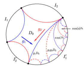
Figure 3.1. Finite Area Surfaces with Cusps

From now on, for the finite area hyperbolic surface $X$, we use the generator given in the above theorem, and denote $\Gamma=\langle g_{1},...,g_{k}\rangle$. Roughly speaking, there are two steps to construct the Ledrappier-Sarig coding. One first uses the generators $\{g_{1},...,g_{k}\}$ to derive a Markov shift $(\Sigma_{1},\sigma_{1})$ (i.e., cutting sequences), then modify $(\Sigma_{1},\sigma_{1})$ to get another Markov shift $(\Sigma_{A},\sigma_{A})$ on which the first returning map has better regularity. We will discuss their construction in detail below.

The shape of the fundamental fundamental $D_{0}$ plays a crucial role in the Ledrappier and Sarig’s coding. We start from looking at vertices of $D_{0}$. Notice that for every vertex $v$ of $D_{0}$, there exists a (shortest) cycle, say $l$ elements, of edge-pairing isometries $g_{s_{i}}$ for $1\leq i\leq l$ such that $v$ is the unique fixed point of $g_{s_{l}}g_{s_{l-1}}...g_{s_{2}}g_{s_{1}}$ provided $g_{s_{i}}...g_{s_{2}}g_{s_{1}}(D_{0})$ and $(g_{s_{1}}^{-1}g_{s_{2}}^{-1}...g_{s_{i}}^{-1})(D_{0})$ touch $\partial_{\infty}\mathbb{D}$ at $v$ for all $1\leq i\leq l$. We call $\underline{w}=(s_{1},...,s_{l})$ and $\underline{w^{\prime}}=(s^{\prime}_{l},....,s^{\prime}_{1})$ the cycles of $v$. We denote the set of all vertex cycles by $\mathfrak{C}$, and $N(\mathcal{\mathfrak{C}})$ is the least common multiplier of length of cycles of all vertices (see Figure 3.1).

3.1.1. The Classical Coding

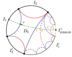
Figure 3.2. Classical Coding

Recall that a vector $v\in T^{1}X$ escapes to infinity if $g_{t}(v)$ leaves, eventually, all compact set $K\subset T^{1}M$ as $t\to\infty$ or $-\infty.$ Let $\Omega_{0}\subset T^{1}X$ be the set of non-escaping vectors. It is clearly that $\Omega_{0}$ is a flow invariant set and contains most of the interesting dynamics.

A unit vector $v\in T^{1}\mathbb{D}$ based at $\mathbb{D}\cap\partial D_{0}$ is called inward pointing if $g_{t}(v)\in{\rm int}(D_{0})$ for sufficiently small $t$. We denote by $(\partial D_{0})_{{\rm in}}$ the set of all inward pointing vectors. It is not hard to see $(\partial D_{0})_{{\rm in}}$ projects to a Poincaré section of $g_{t}:\Omega_{0}\to\Omega_{0}$, by abusing the notation, we also denote this section by $(\partial D_{0})_{{\rm in}}$.

In the following, we recall two equivalent methods of coding of geodesic flows on $\Omega_{0}$: cutting sequences and boundary expansion. To derive the coding, we first label edges of $D_{0}$ in the following manner. For each edge $e$ of $D_{0}$, it determines a boundary interval $I_{s(e)}$ for some $s(e)\in{\mathcal{S}}$ such that $I_{s(e)}$ has the same vertices as $e$ and is on the side of $e$ which does not contain $D_{0}$. We call $s=s(e)\in{\mathcal{S}}$ the external label of $e$, and $s^{\prime}=s^{\prime}(e)$ the internal label of $e$. See Figure 3.2 for an illustration.

Now we are ready to state two canonical coding or Markov partition associated to $(\partial D_{0})_{{\rm in}}$. For every $v\in(\partial D_{0})_{{\rm in}}$ it is determined by

1. Cutting sequence $(x_{k})\in{\mathcal{S}}^{\mathbb{Z}}$ : $x_{k}$ are the internal labels of the edges of $D_{0}$ cut by $g_{t}(v)$ where $k=1$ is the first cut in postive time and $k=0$ is the first cut in non-negative time.

2. Boundary expansion $(y_{k})\in{\mathcal{S}}^{\mathbb{Z}}$: the lift $\widetilde{(g_{t}v)}\subset T^{1}\mathbb{D}$ is a geodesic on $T^{1}\mathbb{D}$ has a attracting limit point (or the ending point) in $\bigcap_{k\geq 1}I_{y_{1},...,y_{k}}^{+}$, and a repelling limit point (or the beginning point) in $\bigcap_{k\leq 0}I_{y_{0},...,y_{k}}^{-}$ where $I_{s_{1},s_{2},...,s_{k}}^{+}=g_{s_{1}}g_{s_{2}}...g_{s_{k-1}}(I_{s^{\prime}_{k}})$ and $I_{s_{1},s_{2},...,s_{k}}^{-}=g_{s_{1}}^{-1}g_{s_{2}}^{-1}...g_{s_{k-1}}^{-1}(I_{s_{k}})$.

It is not hard to see $(x_{k})_{k\in\mathbb{Z}}=(y_{k})_{k\in\mathbb{Z}}$ because all vertices of $D_{0}$ are on $\partial_{\infty}\mathbb{D}$. Thus we can and will interchange in between these two perspectives. In sum, the classical coding means that for every $v\in(\partial D_{0})_{{\rm in}}$, the geodesic $g_{t}(v)$ correspond to an element in

$$\Sigma_{1}:=\{(x_{k})\in\mathcal{S}^{\mathbb{Z}}:x_{k+1}\neq(x_{k})^{\prime}\}$$

and $\sigma_{1}$ is the left shift on $\Sigma_{1}$.

3.1.2. The Modified Coding

As pointed out in [LS08], $(\Sigma_{1},\sigma_{1})$ is not “good” enough for our purpose. For example, the classcal coding is not necessarly one to one, and the first returning map is not regular enough to push the machinery. Thus we need to modify $(\Sigma_{1},\sigma_{1}$) by looking at a smaller section of the flow $g_{t}:\Omega_{0}\to\Omega_{0}$.

Fix a number $n^{*}$ large, set $N^{*}=4n^{*}N(\mathfrak{C})$, and the set of length $N^{*}$ repeating vertiex cycles defined as

$$\mathfrak{C}^{*}:=\{\underset{N^{*}/|\underline{w}|\ {\rm copies}}{\underbrace{(\underline{w},\underline{w},...,\underline{w})}}:\ \underline{w}\in\mathfrak{C}\}.$$

We write $N^{\#}:=\frac{1}{2}N^{*}-1$. Now consider the following set

$$A:=\{y\in\Sigma_{1}:\ \underset{N^{*}}{\underbrace{(y_{-N^{\#},...,}y_{\frac{N^{*}}{2}})}}\notin\mathfrak{C}^{*}\}\subset\Sigma_{1}.$$

The smaller section $S_{A}\subset(\partial D_{0})_{{\rm in}}$ is given by

$$S_{A}:=\{v\in(\partial D_{0})_{{\rm in}}:\ {\rm the\ cutting\ sequence\ of\ }g_{t}(v)\ {\rm is\ in\ }A\}$$

(see Figure 3.3).

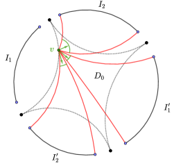
Figure 3.3. The Smaller Section

It is not hard to see that $S_{A}$ is a Poincaré section of $g_{t}:\Omega_{0}\to\Omega_{0}$. Moreover, by the combinatorial property of $\mathfrak{C}$ pointed in [LS08, Section 2.1], we know for a geodesic $g_{t}(v)$ with the cutting sequence $(x_{n})_{n\in\mathbb{Z}}$ which stops returning to $A$ at some point, $(x_{n})$ will eventually repeating an element $\underline{w}\in\mathfrak{C}^{*}$, i.e., $(x_{n})_{n\in\mathbb{Z}}=(....,x_{n},...,\underline{w},\underline{w},\underline{w},...)$.

In other words, if $v$ does not escape to infinity, then the cutting sequence of $g_{t}(v)$ always returns to $A$. More precisely, $\forall x\in A,$ there exists $N=N(x)\in\mathbb{R}$ such that $\sigma_{1}^{N}(x)\in A$. We define the induced shift map on $A$ by $\sigma_{A}(x):=\sigma_{1}^{N_{A}(x)}$ where $N_{A}(x)=\min\{N\in\mathbb{N}:\ \sigma_{1}^{N}(x)\in A\}.$

Now, we are ready to describe a Markov partition of this modified Markov shift $\sigma_{A}:A\to A$:

1. Type I, denoted by $\Sigma_{A}({\rm I})$: cylinders of length $N^{*}+1$, namely $[x_{-N^{\#}},...,\dot{x}_{0},...,x_{\frac{N}{2}^{*}-1},x_{\frac{N}{2}^{*}}]$, such that
   $\underset{{\rm length}=N^{*}}{\underbrace{[x_{-N^{\#}},...,\dot{x}_{0},...,x_{\frac{N}{2}^{*}-1}]}}\subset A$ and $[x_{-N^{\#}+1},...,\dot{x}_{1},...,x_{\frac{N}{2}^{*}}]=\sigma_{1}([x_{-N^{\#}},...,\dot{x}_{0},...,x_{\frac{N}{2}^{*}-1}])\subset A$. The shape of $[\underline{e}]\in\Sigma_{A}({\rm I})$ is defined as $\mathfrak{s}(\underline{e})=(\underline{e})$.

2. Type II, denoted by $\Sigma_{A}({\rm II})$: cylinders of length bigger than $N^{*}+1$, namely

   $$B_{l,k}(a,\underline{w},c):=[x_{-N^{{}^{\#}}},w_{1},...,\dot{w}_{N^{\#}},...,w_{N^{*}},(\underline{w})^{l-1},w_{1},w_{2},...,w_{k},\underline{b}]$$

   where $a:=x_{-N^{\#}},c\in{\mathcal{S}},$ $\underline{w}\in\mathfrak{C}^{*}$, $l\geq 0$, $0\leq k<N^{*}$ are not both zero, and

   $$\underline{b}:=\begin{cases}(w_{k+1},...,w_{N^{*}},w_{1},...,w_{k-1},c)&l=0,k\neq 0\\ (w_{1},...,w_{N^{*}-1},c)&l\neq 0,k=0\\ (w_{k+1},...,w_{N^{*}},w_{1},...,w_{k-1},c)&l,k\neq 0\end{cases}$$

   provided $B_{l,k}(a,\underline{w},c)\subset A$, $[\underline{b}]\subset A$. The shape of $[\underline{e}]\in\Sigma_{A}({\rm II})$ and of the form $B_{l,k}(a,\underline{w},c)$ is deifned as

   $$\mathfrak{s}(\underline{e}):=(k,a,\underline{w},c)\in\{0,...,N^{*}-1\}\times{\mathcal{S}}\times\mathfrak{C}^{*}\times{\mathcal{S}}.$$

Proposition 3.2 ([LS08], Lemma 2.1).

$\sigma_{A}:A\to A$ is topologically mixing, and the Markov partition given by $\Sigma_{A}({\rm I})$ and $\Sigma_{A}({\rm II})$ has the BIP property.

Let $(\Sigma_{A},\sigma_{A})$ be the countable state Markov shift derived by the Markov partition $\Sigma_{A}({\rm I})$ and $\Sigma_{A}({\rm II})$. We write the alphabet set of $\Sigma^{+}_{A}$ by

$${\mathcal{S}}_{A}:=\{\underline{e}\in\bigcup_{n\geq N^{*}+1}{\mathcal{S}}^{n}:\sigma_{1}^{\#}[\underline{e}]\in\Sigma_{A}({\rm I})\cup\Sigma_{A}({\rm II})\}.$$

Let $\pi_{A}:\Sigma_{A}\mapsto A\subset\Sigma_{1}$ denote the natural coding map. For $x\in\Sigma_{A}$, we use $x_{0}$ to denote the letter in the zero-th coordinate. Notice that we can always write $x_{0}=(s_{-N^{\#}},...,s_{n-N^{\#}-1})$ in terms of ${\mathcal{S}}$ letters, and in this representation $n-N^{*}$ is the $\sigma_{1}-$return time of $[x_{0}]$.

Remark 3.3.

1. $\Sigma_{A}({\rm I})$ is composed by return time 1 (i.e., $N_{A}=1)$ cylinders, and $\underset{n+1\ {\rm terms}}{\underbrace{[x_{-N^{\#},...,}x_{n-N^{\#}}]}}\in\Sigma_{A}({\rm II})$ has return time $n-N^{*}$.

2. There are only finitely different shapes $\mathfrak{s}(\underline{a})$ for all $\underline{a}\in{\mathcal{S}}_{A}$.

3. The length $|\underline{a}|$ for $\underline{a}\in{\mathcal{S}}_{A}$ is unbounded.

Recall that every $x=(x_{k})\in\Sigma_{A}$ determines a point $\pi_{A}(x)=(s_{i})\in\Sigma_{1}$, and $\pi_{A}(x)$ corresponds to a unit tangent vector $v(x)\in S_{A}\subset(\partial D_{0})_{{\rm in}}$. We write $\xi(x)$ the attracting limit point of $v(x)$ and $\eta(x)$ the repelling fixed point of $v(x)$. Since $\xi(x)=\bigcap_{k\geq 1}I_{s_{1},...,s_{k}}^{+}$and $\eta(x)=\bigcup_{k\leq 0}I_{s_{0},...,s_{k}}^{-}$ where $\pi_{A}(x)=(s_{i})_{i\in\mathbb{Z}}$, we know that $\xi(x)$ only depends on $x^{+}=(x_{k})_{k\geq 0}$ and $\eta(x)$ only depends on $x^{-}=(x_{k})_{k\leq 0}$ .

Definition 3.4.

The geometric potential $\tau:\Sigma_{A}\to\mathbb{R}$ is defined as

$$\tau(x):=B_{\xi(x)}(o,(g_{x_{0}})o)$$

where $o$ is the origin, $x_{0}=(s_{-N^{\#}},...,s_{n-N^{\#}-1})\in{\mathcal{S}}_{A}$, and $g_{x_{0}}=g_{s_{1}}\circ...\circ g_{s_{n-N^{*}}}$.

Proposition 3.5 (Geometric Potential (I), [LS08], Lemma 2.2).

Let $(\Sigma_{A},\sigma_{A})$ be the Markov shift constructed above. Then

1. Suppose $v$ generates a closed geodesics, namely $g_{l(v)}v=v,$ then there exists a unique (up to permutations) $x=(\overline{x_{1}x_{2}...x_{m}})\in{\rm Fix}^{m}(\Sigma_{A})$ such that $l(v)=S_{m}\tau(x)$, and vice versa.

2. $\tau$ is locally Hölder continuous.

3. $\tau$ only depends on the future coordinates, i.e., if $x_{0}^{\infty}=y_{0}^{\infty}$ then $\tau(x)=\tau(y)$.

4. $\exists C,K>0$ such that $\tau(x)+\tau(\sigma(x))+...+\tau(\sigma^{n}(x))\geq C$ for all $n\geq K$.

Since the geometric potential $\tau$ is only dependent on the future coordinate, we can focus on $(\Sigma^{+}_{A},\sigma_{A})$ the one-sided countable Markov shift deduced from $(\Sigma_{A},\sigma_{A})$ by forgetting the past coordinate.

Proposition 3.6 (Geometric Potential (II), [LS08], Lemma 3.1).

On the one-sided countable Markov shift $(\Sigma^{+}_{A},\sigma_{A})$, we have

1. $\tau$ has a unique equilibrium state $m_{-\tau}$ and $\int_{\Sigma^{+}_{A}}\tau\,\mathrm{d}m_{-\tau}<\infty$.

2. The Liouville measure $m_{L}$ on $T^{1}X$ is given by $m_{L}=R(m_{-\tau})\circ\widetilde{\pi}_{A}^{-1}$ where $R:{\mathcal{\mathcal{M}}_{\sigma}\to{\mathcal{M}}_{\tau}}$ given in Theorem 2.15.

3. $P(-\tau)=0$.

4. $\tau$ is bounded on $\Sigma_{A}({\rm I})$, and there exists $C_{1}>0$ such that $2\ln|x_{0}|-C_{1}\leq\tau(x)\leq 2\ln|x_{0}|+C_{1}$ for all $x\in\Sigma_{A}({\rm II})$.

Proof.

Everything is in [LS08, Lemma 3.1], and only the first assertion of (4) needs more explorations. Let $[x_{0}]\in\Sigma_{A}({\rm I)}$ and $x\in[x_{0}]$. We can write $x_{0}=(s_{-N^{\#}},...,s_{\frac{N^{*}}{2}-1},s_{\frac{N^{*}}{2}})$, $g_{x_{0}}(x)=g_{s_{1}}$, and $\tau(x)=B_{\xi(x)}(o,g_{s_{1}}o)$ where $s_{i}\in{\mathcal{S}}$ for $i=-N^{\#},...,\frac{N^{*}}{2}$. Recall that in the disc model, $B_{\xi}(o,y)=\ln\frac{1-|y|^{2}}{|\xi-y|^{2}}$. Since $\xi(x)\in I_{s_{1},s_{2},...,s_{\frac{N^{*}}{2}}}^{+}$, it is not hard to see $B_{\xi(x)}(o,g_{s_{1}}o)=\ln(\frac{1-|g_{s_{1}}o|^{2}}{|\xi(x)-g_{s_{1}}o|})$ is (uniformly) bounded for all $x\in[x_{0}]$. Notice that this bound depends on $[x_{0}]\in\Sigma_{A}({\rm I}).$ We can find a universal bound $\tau(x)$ on $\Sigma_{A}({\rm I})$ because $|\Sigma_{A}({\rm I})|<\infty$. ∎

Remark 3.7.

1. By standard techniques in symbolic dynamics, we know $\tau$ is cohomologus to $\tau^{\prime}$ which is locally Hölder and bounded away from zero (cf. [Kao18, Lemma 3.8]). From now on, we will use $\tau^{\prime}$ to replace $\tau$ whenever $\tau$ needs to be bounded away from zero. Abusing the notation, we will continue denote $\tau^{\prime}$ by $\tau$.

2. In [LS08], the constant $C_{1}$ in Proposition 3.6 (4) depends on the shape of $x_{0}$. Because there are only finitely many shapes, we can replace it by a universal constant.

3.2. Type-preserving Finite Area Fuchsian Representations

In the this subsection, we consider $\rho_{1},\rho_{2}$ two type-preserving finite area Fuchsian representations. The Fenchel-Neilsen Isomorphism Theorem (cf. Theorem 2.1) shows that there exists a bilipschitz map taking the limit set $\Lambda(\rho_{1}(\pi_{1}S))$ and fundamental domain of $X_{\rho_{1}}$ to $\Lambda(\rho_{2}(\pi_{1}S))$ and the fundamental domain of $X_{\rho_{2}}$, and hence $\Lambda_{0}(\rho_{1})$ to $\Lambda_{0}(\rho_{2})$. Hence, the suspension flows corresponding the geodesic flows on $\Omega_{0}(\rho_{1})$ and $\Omega_{0}(\rho_{2})$ correspond to the same Markov shift $(\Sigma^{+}_{A},\sigma_{A})$ but different roof functions $\tau_{\rho_{1}}$, $\tau_{\rho_{2}}$, respectively. The following result shows that we have a nice control of these roof functions.

Corollary 3.8.

There exists $C>0$ such that $|\tau_{\rho_{1}}(x)-\tau_{\rho_{2}}(x)|<C$ for all $\Sigma^{+}_{A}$.

Proof.

It follows immediately from Proposition 3.6 (4). ∎

In the second part of this subsection, we discuss the intersection number ${\rm I}(\rho_{1},\rho_{2})$ of $\rho_{1}$ and $\rho_{2}$ proposed by Thurston. Recall that ${\rm I}(\rho_{1},\rho_{2})$ of $\rho_{1}$ and $\rho_{2}$ is defined as

$${\rm I}(\rho_{1},\rho_{2}):=\lim_{n\to\infty}\frac{l_{2}[\gamma_{n}]}{l_{1}[\gamma_{n}]}$$

where $\{[\gamma_{n}]\}_{n=1}^{\infty}$ is a sequence of conjugacy classes for which the associated closed geodesics $\gamma_{n}$ become equidistributed on $\rho_{1}(\pi_{1}S)\backslash\mathbb{H}$ with respect to the Liouville measure. However, it is unclear why ${\rm I}(\rho_{1},\rho_{2})$ is well-defined, especially, when $S$ has punctures. We will discuss this issue in Proposition 3.9 where we give ${\rm I}(\rho_{1},\rho_{2})$ a dynamics characterization.

We now can state and prove the main result of this subsection: characterizing ${\rm I}(\rho_{1},\rho_{2})$ by the symbolic model.

Proposition 3.9.

Suppose $\rho_{1},\rho_{2}$ are two type-preserving finite area Fuchsian representations. Then the intersection ${\rm I}(\rho_{1},\rho_{2})$ is well-defined. Moreover, if $\tau$, $\kappa$ are the geometric potential for $\rho_{1}$, $\rho_{2}$, respectively, then

$${\rm I(\rho_{1},\rho_{2})=}\frac{\int\kappa\,\mathrm{d}m_{-\tau}}{\int\tau\,\mathrm{d}m_{-\tau}}$$

where $m_{-\tau}$ is the equilibrium state of $\tau$.

Proof.

Since the lifted measure $R(m_{-\tau})$ on $\Sigma_{\tau}^{+}$ is the unique measure of maximum entropy, we know it ergodic. Plus $(\Sigma^{+}_{A},\sigma_{A})$ is topologically mixing, we know $R(m_{-\tau})$ is the weak-start limit of some period orbits $\{\lambda_{n}\}\subset\Sigma^{+}_{\tau}$, that is, $\frac{\delta_{\lambda_{n}}}{l(\lambda_{n})}\overset{weak^{*}}{\longrightarrow}R(m_{-\tau})$ where $\lambda_{n}=\{(x_{n},t)\in\Sigma^{+}_{\tau}:\ 0\leq t\leq S_{m}\tau(x_{n}),\ x_{n}\in{\rm Fix}^{m}\ {\rm for}\ {\rm some\ }m\}$, $\delta_{\lambda_{n}}$ is the Dirac measure on $\lambda_{n}$, and $l(\lambda_{n}):=S_{m}\tau(x_{n})=l_{1}[\gamma_{n}]$ with $\gamma_{n}\in\pi_{1}S$ the hyperbolic elements corresponding to $\lambda_{n}$.

Let us consider the (symbolic) reparametrization function $\psi(x,t)=\frac{\kappa(x)}{\tau(x)}$ for $0\leq t\leq\tau(x)$ . By Proposition 3.6 and Corollary 3.8, we know $\psi$ is a bounded locally Hölder continuous function such that $\int_{\rho_{1}(\gamma_{n})}\psi(\phi_{t})\,\mathrm{d}t=l_{2}[\gamma_{n}]$. Thus ,

$$\left.\frac{\langle\delta_{o_{n}},\psi\rangle}{l(o_{n})}\right|_{\Sigma^{+}_{\tau}}=\frac{l_{2}[\gamma_{n}]}{l_{1}[\gamma_{n}]}\to\int_{\Sigma^{+}_{\tau}}\psi\,\mathrm{d}R(m_{-\tau})=\frac{\int_{\Sigma^{+}}\kappa\,\mathrm{d}m_{-\tau}}{\int_{\Sigma^{+}}\tau\,\mathrm{d}m_{-\tau}}$$

where the last equality follows Theorem 2.15. ∎

4. Phase Transitions for Geodesic Flows

Through out this section, let $\rho_{1}$ and $\rho_{2}$ be two type-preserving finite volume Fuchsian representations, and we write $X_{1}=\Gamma_{1}\backslash\mathbb{D}$ and $X_{2}=\Gamma_{2}\backslash\mathbb{D}$ where $\Gamma_{1}=\rho_{1}(\pi_{1}(S))$ for $i=1,2$. Following the above section, let $(\Sigma^{+},\sigma)=(\Sigma^{+}_{A},\sigma_{A})$ be the Markov shift associated with $X_{1}$ and $X_{2}$, and we denote their geometric potentials by $\tau$ and $\kappa$, respectively.

To derive the analyticity of pressure, we need to locate the place where phase transition happens. As in [Kao18], we have the following observation.

Theorem 4.1 (Phase Transition).

Suppose $a,b\geq 0$, $a+b\neq 0$, and $\tau,\kappa$ are given above. Then we have

$$P(-t(a\tau+b\kappa))=\begin{cases}{\rm analytic}&t>\frac{1}{2(a+b)},\\ \infty&t<\frac{1}{2(a+b)}.\end{cases}$$

Moreover, there exists a unique $t_{ab}\in(\frac{1}{2(a+b)},\infty)$ such that $P(-t_{a,b}(a\tau+b\kappa))=0$.

Proof.

By Theorem 2.11, we know it is sufficient to show

$$P(-t(a\tau+b\kappa))=\begin{cases}{\rm finite}&t>\frac{1}{2(a+b)},\\ \infty&t<\frac{1}{2(a+b)}.\end{cases}$$

Recall [MU03, Theorem 2.19], we know for any locally Hölder continuous function $f$, $P(f)<\infty$ if and only if

$$Z_{1}(f):=\sum_{x_{0}\in{\mathcal{S}}_{A}}e^{\sup\{f(x):x\in[x_{0}]\}}<\infty.$$

By Proposition 3.6, there exists constants $C_{1}$, $C_{2}>0$ such that

$$Z_{1}(-t(a\tau+b\kappa))= \sum_{x_{0}\in\Sigma_{A}({\rm I})}e^{\sup\{-t(a\tau+b\kappa):x\in[x_{0}]\}}+\sum_{x_{0}\in\Sigma_{A}({\rm II})}e^{\sup\{-t(a\tau+b\kappa):x\in[x_{0}]\}}$$

$$\leq C_{1}+\sum_{x_{0}\in\Sigma_{A}({\rm II})}\sum_{|x_{0}|=N^{*}+1}^{\infty}e^{-2t(a\tau+b\kappa))\log|x_{0}|+C}$$

$$= C_{1}+C_{2}\sum_{x_{0}\in\Sigma_{A}({\rm II})}\sum_{|x_{0}|=N^{*}+1}^{\infty}e^{-2t(a\tau+b\kappa))\log|x_{0}|}.$$

Similarly, there exists constants $C_{3}$, $C_{4}>0$ such that

$$Z_{1}(-t(a\tau+b\kappa))\geq C_{3}+C_{4}\sum_{x_{0}\in\Sigma_{A}({\rm II})}\sum_{|x_{0}|=N^{*}+1}^{\infty}e^{-2t(a\tau+b\kappa))\log|x_{0}|}.$$

Thus, it is clear that $Z_{1}(-t(a\tau+b\kappa))<\infty$ if and only if $t>\frac{1}{2(a+b)}$.

Lastly, fix $a,b$ with $a,b\geq 0,a+b\neq 0$, then the computation in [MU03, Theorem 2.19] showed that, in our case, $Z_{1}(-t(a\tau+b\kappa))\to\infty$ as $t\to\frac{1}{2(a+b)}$ implies $P(-t(a\tau+b\kappa))\to\infty$ as $t\to\frac{1}{2(a+b)}$. In particular, taking $t$ close to $\frac{1}{2(a+b)}$, we have $P(-t(a\tau+b\kappa))>0$. Moreover, it is obvious that $P(-t(a\tau+b\kappa))<0$ when $t$ is big enough. Hence, by the analyticity and the monotonicity of the pressure, we know there exists a unique $t_{a,b}$ such that $P(-t_{a,b}(a\tau+b\kappa))=0$. ∎

Corollary 4.2.

The set $\{(a,b):\ a,b\geq 0,a+b\neq 0,{\rm\ and}\ P(-a\tau-b\kappa)=0\}$ is a real analytic curve.

Proof.

The proof of [Kao18, Theorem 3.14] applies to here. In short, by Theorem 4.1, it makes sense to discuss solutions to $P(-a\tau-b\kappa)=0$. To see the solution set is a real analytic curve one only needs to apply the Implicit Function Theorem, because we know

$$\left.\partial_{b}P(-a\tau-b\kappa)\right|_{(a_{0},b_{0})}=-\int\kappa\,\mathrm{d}\nu_{-a_{0}\tau-b_{0}\kappa}<-c$$

where $c>0$ is a lower bound for $\kappa$ and $\nu_{-a_{0}\tau-b_{0}\kappa}$ is the Gibbs measure for $-a_{0}\tau-b_{0}\kappa$. ∎

5. Manhattan Curves, Critical Exponents, and Rigidity

In this section, we will prove Theorem A and Theorem B. The ideas most follow [Kao18]. In [Kao18], the author used results of Paulin, Pollicott and Schapira [PPS15] to analyze the geometric Gurevich pressure over the geodesics flow. The general frame work in [PPS15] includes finite area hyperbolic surfaces. Nevertheless, for the completeness, we will give outlines of the proofs, and reader can find all details in [Kao18].

Following the notations in Section 4, let $\rho_{1},\rho_{2}$ be two type-preserving finite area Fuchsian representations, $X_{1}=X_{\rho_{1}}$ and $X_{2}=X_{\rho_{2}}$ be the corresponding hyperbolic surfaces, and $\tau$,$\kappa$ be the corresponding geometric potentials over the Markov shift $(\Sigma^{+},\sigma)=(\Sigma^{+}_{A},\sigma_{A})$. Recall that the Poincaré series $Q_{\rho_{1},\rho_{2}}^{a,b}(s)$ of the weighted Manhattan metric $d_{\rho_{1},\rho_{2}}^{a,b}$ is defined by

$$Q_{\rho_{1},\rho_{2}}^{a,b}(s):=\sum_{\gamma\in\pi_{1}(S)}\exp(-s\cdot d_{\rho_{1},\rho_{2}}^{a,b}(o,\gamma o)),$$

$\delta_{\rho_{1},\rho_{2}}^{a,b}$ is the critical exponent of $Q_{\rho_{1},\rho_{2}}^{a,b}$, and the Manhattan curved ${\mathcal{C}}(\rho_{1},\rho_{2})$ of $\rho_{1}$ and $\rho_{2}$ is the set $\{(a,b)\in\mathbb{R}_{\geq 0}\times\mathbb{R}_{\geq 0}\backslash(0,0):\ {\displaystyle\delta_{\rho_{1},\rho_{2}}^{a,b}=1\}}$. For the brevity, we will drop the subscript $\rho_{1},\rho_{2}$ in the rest of this subsection.

The goal of this subsection is to prove the following theorem:

Theorem 5.1.

[Kao18, Section 4] Suppose $a,b\geq 0$ and $ab\neq 0$, then

$$P(-\delta_{\rho_{1},\rho_{2}}^{a,b}(a\tau+b\kappa))=0.$$

In particular, $(a,b)\in{\mathcal{C}}(\rho_{1},\rho_{2})$ if and only if the pair $(a,b)$ satisfies $P(-a\tau-b\kappa)=0$.

Proof.

As we mentioned before results in [Kao18, Section 4] are applicable here. Here we give a brief outline of the proof. We consider following growth rates and their relations:

• the geometric Gurevich pressure $P_{{\rm Geo}}^{a,b}$ given by growth rates of closed orbits on $T^{1}X_{1}$:

  $$P_{{\rm Geo}}^{a,b}:={\displaystyle\limsup_{s\to\infty}\frac{1}{s}\log Z_{W}(s)}$$

  where $Z_{W}(s):={\displaystyle\sum_{\stackrel{{\scriptstyle[}}{{\lambda}}\in{\rm Per}_{1}(s)]{\lambda\cap W\neq\phi}{}}e^{-al_{1}[\lambda]-bl_{2}[\lambda]}}$ where $W\subset T^{1}X_{1}$ is a relatively compact open set and ${\rm Per}_{1}(s):=\{\lambda:\ \mbox{$\lambda\ $is a closed orbit on }T^{1}X_{1}{\rm\ and\ }l_{1}[\lambda]\leq s\}$.

• the critical exponent $\overline{\delta}^{a,b}$ proposed in [PPS15]: $\overline{\delta}^{a,b}$ is the critical exponent of $Q_{{\rm PPS},x,y}^{a,b}(s):={\displaystyle\sum_{\gamma\in\pi_{1}(S)}e^{-d^{a,b}(x,\gamma y)-sd(x,\rho_{1}(\gamma)y)}}$ the Paulin-Pollicott-Schapira’s (PPS) Poincaré series.

• Let $\psi(x,t):=\frac{\kappa(x)}{\tau(x)}:\Sigma^{+}_{\tau}\to\mathbb{R}$ for $t\in[0,\tau(x)]$. Then [Kao18, Lemma 4.7] showed that $P_{\phi}(-a-b\psi)=0\iff P(-a\tau-b\kappa)=0$.

• [Kao18, Lemma 4.3, 4.4] showed that $P_{{\rm Geo}}^{a,b}=\overline{\delta}^{a,b}=P_{\phi}(-a-b\psi).$

• [Kao18, Lemma 4.5] pointed out that $\overline{\delta}^{a,b}=0\iff\delta^{a,b}=1$.

In sum, we have

$$\delta^{a,b}=1 \iff\overline{\delta}^{a,b}=0$$

$$\iff P_{{\rm Geo}}^{a,b}=0$$

$$\iff P_{\phi}(-a-b\psi)=0$$

$$\iff P(-a\tau-b\kappa)=0.$$

Thus, $P(-t_{a,b}(a\tau+b\kappa))=0\iff\delta^{t_{a,b}a,t_{a,b}b}=1$ , i.e. $Q_{{\rm PPS},o,o}^{t_{a,b}a,t_{a,b}b}(s)={\displaystyle\sum_{\gamma\in\pi_{1}(S)}e^{-t_{ab}d^{a,b}(o,\gamma o)}}$ has critical exponent 1. Hence, $Q_{{\rm PPS},o,o}^{t_{a,b}a,t_{a,b}b}(s)={\displaystyle\sum_{\gamma\in\pi_{1}(S)}e^{-sd^{a,b}(o,\gamma o)}}$ has critical exponent $t_{a,b}$, and thus, $\delta^{a,b}=t_{a,b}$. ∎

By Corollary 4.2 and the above theorem, we have:

Corollary 5.2.

The Manhattan curve ${\mathcal{C}}(\rho_{1},\rho_{2})$ is a real analytic curve give by, for $a,b\geq 0$ and $a+b\neq 0$,

$${\mathcal{C}}(\rho_{1},\rho_{2})=\{(a,b):\ P(-a\tau-b\kappa)=0\}.$$

The following theorem is Bowen’s formula which characterize the topological entropy of the geodesic flow by the pressure and the geometric potential.

Corollary 5.3.

Suppose $\rho_{1}$ is a finite volume Fuchsian representation $\rho_{1}$. Then

$$P(-1\cdot\tau)=0$$

where $1$ is the critical exponent of $\rho_{1}(\pi_{1}(S))$.

Proof.

It follows Proposition 3.6 and the fact that when $\rho_{1}$ is a finite area Fuchsian representation then the critical exponent of $\rho_{1}(\pi_{1}(S))$ is 1 (cf. [OP04]). ∎

Notice that by Bowen’s formula and the Implicit Function Theorem, we can prove that the pressure varies analytically when $\tau$ varies analytically with $P(-\tau)=0$.

Now we are ready to prove Theorem A.

Theorem 5.4 (Theorem A).

The ${\mathcal{C}}(\rho_{1},\rho_{2})$ is a convex real analytic curve. Moreover, ${\mathcal{C}}(\rho_{1},\rho_{2})$ is strictly convex unless $\rho_{1}$ and $\rho_{2}$ are conjugate in ${\rm PSL}(2,\mathbb{R})$, in such cases ${\mathcal{C}}(\rho_{1},\rho_{2})$ is a straight line.

Proof.

The analyticity of ${\mathcal{C}}$ is proved in Corollary 5.2. To show the remaining parts, we first notice that by Hölder’s inequality the Manhattan curve ${\mathcal{C}}$ is always convex, and because ${\mathcal{C}}$ is real analytic we know ${\mathcal{C}}$ is either a straight line or strictly convex. It is clear that if $\rho_{1}$ and $\rho_{2}$ are conjugate then ${\mathcal{C}}$ is a straight line. We claim that if ${\mathcal{C}}$ is a straight line then $\rho_{1}$ and $\rho_{2}$ are conjugate in ${\rm PSL}(2,\mathbb{R})$.

To see this, suppose ${\mathcal{C}}$ is a straight line. Then the slope of this line is $-1$ because $(1,0)$,$(0,1)\in{\mathcal{C}}$. In other words, we have

(5.1) $$-1=-\frac{\int\tau\,\mathrm{d}m_{-\tau}}{\int\kappa\,\mathrm{d}m_{-\tau}}=-\frac{\int\tau\,\mathrm{d}m_{-\kappa}}{\int\kappa\,\mathrm{d}m_{-\kappa}}$$

where $m_{-\tau}$, $m_{-\kappa}$ are the equilibrium states for $-\tau$ and $-\kappa$, respectively.

It is sufficient to show that $\tau$ and $\kappa$ are cohomologus, because $\tau\sim\kappa$ implies that $X_{1}$ and $X_{2}$ has the same marked length spectrum, and which implies that $\rho_{1}$ and $\rho_{2}$ are conjugate in $\mathrm{PSL}(2,\mathbb{R})$ (cf. Theorem 2.3).

To see $\tau$ and $\kappa$ are cohomologus, by Theorem 2.10, it is enough to show $m_{-\tau}=m_{-\kappa}$. Notice that $m_{-\tau}$, $m_{-\kappa}$ are the equilibrium state of $-\tau$, $-\kappa$, respectively, we have

$$h_{\sigma}(m_{-\tau})-\int\tau\,\mathrm{d}m_{-\tau}=P(-\tau)=0=P(-\kappa)=h_{\sigma}(m_{-\kappa})-\int\kappa\,\mathrm{d}m_{-\kappa}.$$

Moreover, by equation $($5.1$)$, we know $\int\kappa\,\mathrm{d}m_{-\tau}=\int\tau\,\mathrm{d}m_{-\tau}$. Thus, we get

$$h_{\sigma}(m_{-\tau})+\int(-\kappa)\,\mathrm{d}m_{-\tau}=0=P(-\kappa).$$

In other words, $m_{-\tau}$ is a equilibrium state for $-\kappa$, and by the uniqueness of equilibrium states, we get $m_{-\kappa}=m_{-\tau}$. ∎

Using the strictly convexity of the Manhattan curve, we have the following rigidity results.

Theorem 5.5 (Bishop-Steiger Rigidity; Theorem B).

Suppose $\rho_{1},\rho_{2}$ is two type-preserving finite volume Fuchsian representations. Then $h_{{\rm BS}}(\rho_{1},\rho_{2})\leq\frac{1}{2}$. Moreover, the equality holds if and only if $\rho_{1}$ and $\rho_{2}$ are conjugate in $\mathrm{PSL}(2,\mathbb{R})$.

Proof.

We first notice that it is a standard and well-known procedure (cf. [Kao18, Theorem 4.8]) to show

$$\delta^{1,1}=h_{{\rm BS}}=\lim_{T\to\infty}\frac{1}{T}\ln\left(\#\{[\gamma]\in[\pi_{1}(S)]:d(o,\rho_{1}(o,\gamma o)+d(o,\rho_{2}(o,\gamma o)\leq T\}\right).$$

Moreover, since $(\frac{1}{2},\frac{1}{2})$ is the middle point of $(0,1),(1,0)\in{\mathcal{C}}(\rho_{1},\rho_{2})$, by Theorem 5.4, we know $(\frac{1}{2},\frac{1}{2})$ is above $\delta^{1,1}\cdot(1,1)\in{\mathcal{C}}(\rho_{1},\rho_{2})$ and $\delta^{1,1}=\frac{1}{2}$ if and only if ${\mathcal{C}}$ is a straight line. ∎

Theorem 5.6 (Thurston’s Rigidity; Theorem B).

Suppose $\rho_{1},\rho_{2}$ is two type-preserving finite volume Fuchsian representations. Then

$${\rm I}(\rho_{1},\rho_{2})\geq 1$$

and equals to 1 if and only if $\rho_{1}$ and $\rho_{2}$ are conjugate in $\mathrm{PSL}(2,\mathbb{R})$.

Proof.

By Proposition 3.9, we know

$${\rm I}(\rho_{1},\rho_{2})=\frac{\int\kappa\,\mathrm{d}m_{-\tau}}{\int\tau\,\mathrm{d}m_{-\tau}}.$$

Recall that $m_{-\kappa}$ is the equilibrium state of $-\kappa$ and $m_{-\tau}\in{\mathcal{M}}_{\sigma}$ we have

$$0=P(-\kappa)=h_{\sigma}(m_{-\kappa})-\int\kappa\,\mathrm{d}m_{-\kappa}\geq h_{\sigma}(m_{-\tau})-\int\kappa\,\mathrm{d}m_{-\tau}.$$

Notice that $m_{-\tau}$ is the equilibrium state of $-\tau$, i.e., $0=P(-\tau)=h_{\sigma}(m_{-\tau})-\int\tau\,\mathrm{d}m_{-\tau}$, we have

$$\int\tau\,\mathrm{d}m_{-\tau}=h_{\sigma}(m_{-\tau})\leq\int\kappa\,\mathrm{d}m_{-\tau}.$$

The rigidity part has proved in Theorem 5.4. More precisely, we proved in Theorem 5.4 that if $1=\frac{\int\kappa\,\mathrm{d}m_{-\tau}}{\int\tau\,\mathrm{d}m_{-\tau}}$ then $\rho_{1}\sim\rho_{2}$ in $\mathrm{PSL}(2,\mathbb{R})$. ∎

6. The Pressure Metric

6.1. The Pressure Metric and Thurston’s Riemannian Metric

The aim of this subsection is to construct a Riemannian metric for the Teichmüller space of surfaces with punctures. Using the symbolic model of geodesics flows discussed in Section 3, we can relate the Teichmüller space with the space of geometric potentials.

Recall that $S=S_{g,n}$ is an orientable surface of $g$ genus and $n$ punctures and with negative Euler characteristic. The Teichmüller space ${\mathcal{T}}(S)$ is the space of conjugacy classes of finite area type-preserving Fuchsian representations. By Section 3, we know that for every $\rho\in{\mathcal{T}}(S)$, the geodesics flow on a smaller section $\Omega_{0}\subset T^{1}X_{\rho}$ conjugates the suspension flow over a Markov shift $(\Sigma^{+},\sigma)=(\Sigma^{+}_{A},\sigma_{A})$ with a unique (up to cohomologacy) locally Hölder continuous roof function $\tau$. We want to point out again that the Markov shift $(\Sigma^{+},\sigma)$ is constructed through the shape of fundamental domain. Since type-preserving Fuchsian representations have the same shape of fundamental domain, we know the suspension flow models for all $\rho\in{\mathcal{T}}(S)$ have the same base space $(\Sigma^{+},\sigma)$ yet with different roof functions.

Let $\mathtt{\mathbf{P}}$ be the set of pressure zero locally Hölder continuous functions on $\Sigma^{+}$, that is,

$$\mathbf{\mathbf{P}}:=\{\tau\in C(\Sigma^{+}):\tau{\rm\ is\ locally\ H\ddot{o}lder,\ }P(-\tau)=0\}.$$

In the following, we will discuss the relations between ${\mathcal{T}}(S)$ and $\mathtt{\mathbf{P}}$. Notice that since ${\mathcal{T}}(S)$ is composed by representations in $\mathrm{PSL}(2,\mathbb{R})$, it inherits a natural analytic structure from $\mathrm{PSL}(2,\mathbb{R})$ (see [Ham03] for more details). The following proposition indicates that there exists an analytic thermodynamic mapping $\Phi:{\rm Hom_{tp}^{F}}(\pi_{1}(S),{\rm PSL}(2,\mathbb{R}))\to\mathbf{\mathbf{P}}$.

Proposition 6.1 (Thermodynamic Mapping).

Let $0<\varepsilon\ll 1$ and $\{\rho_{t}\}_{t\in(-\varepsilon,\varepsilon)}\subset{\mathcal{T}}(S)$ be an analytic one-parameter family in ${\mathcal{T}}(S)$, then $\Phi(\{\rho_{t}\})=\{\tau_{t}\}\subset\mathbf{\mathbf{P}}$ is an analytic one-parameter family in $\mathbf{\mathbf{P}}$.

Proof.

We first notice that if $\{\rho_{t}\}\subset{\mathcal{T}}(S)$ is analytic then the boundary map (derived in Theorem 2.1) ${\rm b}_{t}:\partial_{\infty}\mathbb{H}=\Lambda(\rho_{0}(\pi_{1}S))\to\Lambda(\rho_{t}(\pi_{1}S))=\partial_{\infty}\mathbb{H}$ is real analytic (see [McM08, Section 2] or [BCS18, Proposition 4.1]). For the completeness, we summarize the proof of this fact. The idea of [McM08, Section 2], as well as [BCS18, Proposition 4.1], is a complex analytic approach, namely, using holomorphic motions and the $\lambda-$lemma.

Let us denote $QF(S)$ the space conjugacy classes of quasi-Fuchsian (i.e., the limit set is a Jordan curve) representations of $\pi_{1}(S)\to{\rm\mathrm{PSL}(2,\mathbb{C})}$. Recall that $QF(S)$ is an open neighborhood of ${\mathcal{T}}(S)$ in the $\mathrm{PSL}(2,\mathbb{C})-$character variety of $\pi_{1}(S)$. Let $\rho_{t}$ vary in $QF(S)$, then there exist an embedding $\overline{{\rm b}}_{t}:\partial_{\infty}\mathbb{H}\to\Lambda(\rho_{t}(\pi_{1}S)\subset\hat{\mathbb{C}}$. Notice that $\rho_{0}\in{\mathcal{T}}(S)$ is fixed. It is clear that if $\xi\in\Lambda(\rho_{0}(\pi_{1}S))$ is fixed by a nontrivial element $\rho_{0}(\gamma)$, then $b_{t}(\xi)$ varies holomorphically. Thus by Slodkowski’s generalized $\lambda-$lemma (cf. [Slo91]), we know $\overline{{\rm b}}_{t}$ varies complex analytically when $\rho_{t}$ varies in $QF(S)$; hence, ${\rm b}_{t}(={\rm\overline{b}_{t}})$ varies real analytically when $\rho_{t}$ varies in ${\mathcal{T}}(S)$.

To see $\{\tau_{t}\}$ is real analytic, by definition

$$\tau_{t}(x)=B_{\xi_{t}(x)}(o,\rho_{t}(g_{x_{0}})o)$$

where $x=x_{0}...$, and $\xi_{t}={\rm b}_{t}\circ\xi_{0}:\Sigma^{+}\to\Lambda(\rho_{t}(\pi_{1}S))$. Recall that in the disk model, we know $B_{\xi}(x,y)=\ln(\frac{1-|y|^{2}}{|\xi-y|^{2}}\frac{|\xi-x|^{2}}{1-|x|^{2}})$. Thus we have, without loss of generality, taking $o$ to be the origin,

$$\tau_{t}(x)=B_{{\rm b}_{t}\circ\xi_{0}}(o,\rho_{t}(g_{x_{0}})o)=\ln\frac{1-|\rho_{t}(g_{x_{0}})o|^{2}}{|{\rm b}_{t}\circ\xi_{0}(x)-\rho_{t}(g_{x_{0}})o|^{2}}.$$

Since both $\rho_{t}$ and $b_{t}$ vary real analytically, from the above expression we know $\tau_{t}$ also varies real analytically. ∎

By Corollary 3.8 we know that $\tau_{\rho_{1}}$ is locally Hölder continuous and $|\Phi(\rho_{1})-\Phi(\rho_{0})|=|\tau_{\rho_{1}}-\tau_{\rho_{0}}|$ is bounded for all $\rho_{0},\rho_{1}\in{\mathcal{\mathcal{T}}}(S)$. Thus, consider an analytic path $\rho_{t}\subset{\mathcal{T}}(S)$, and we write out the analytic path $\tau_{t}=\Psi(\rho_{t})$, in terms of Taylor expansion, $\tau_{t}=\tau_{0}+t\cdot\dot{\tau}_{0}+...$. We know the perturbation $\dot{\tau}_{0}$ is a bounded locally Hölder continuous function. Therefore, it is sufficient to consider $T_{\tau_{0}}\mathbf{P}$, the corresponding tangent space of $T_{\rho_{0}}{\mathcal{T}}(S)$, as

$$T_{\tau_{0}}\mathbf{P}:=\{f\in C(\Sigma^{+}):\int_{\Sigma^{+}}f\,\mathrm{d}m_{-\tau_{0}}=0,f{\rm\ is\ locally\ H\ddot{o}lder\ and\ bounded}\}\subset{\rm Ker}D_{-\tau_{0}}P.$$

Moreover, we are interested in the pressure norm $||\cdot||_{P}$ on $\mathbf{P}$ given by

$$||f||_{{\rm P}}:=\frac{{\rm Var}(f,m_{-\tau_{0}})}{\int\tau_{0}\,\mathrm{d}m_{-\tau_{0}}}.$$

Notice that this norm degenerates precisely when $f\sim 0$. In the theorem below, we prove that one can define the pressure metric $||\cdot||$ on ${\mathcal{T}}(S_{g,n})$ through $||\cdot||_{P}$:

Theorem 6.2 (Theorem C).

Suppose $0<\varepsilon\ll 1$ and $\rho_{t}\in{\mathcal{T}}(S_{g,n})$ is an analytic path for $t\in(-\varepsilon,\varepsilon)$. Then ${\rm I}(\rho_{0},\rho_{t})$ is real analytic and

$$||\dot{\rho}_{0}||^{2}:=||d\Psi(\dot{\rho}_{0})||_{{\rm P}}^{2}=\left.\frac{{\rm d}^{2}{\rm I}(\rho_{0},\rho_{t})}{{\rm d}t^{2}}\right|_{t=0}$$

defines a Riemannian metric on ${\mathcal{T}}(S_{g,n})$.

Proof.

Follows Proposition 3.9 and Proposition 6.1, we know ${\rm I}(\rho_{0},\rho_{t})$ is real analytic. Thus, it is sufficient to show that $\left.\frac{{\rm d}^{2}{\rm I}(\rho_{0},\rho_{t})}{{\rm d}t^{2}}\right|_{t=0}=||d\Psi(\dot{\rho}_{0})||_{{\rm P}}^{2}$ and $||d\Psi(\dot{\rho}_{0})||_{{\rm P}}^{2}>0$ when $\dot{\rho}_{0}\neq 0$.

By Proposition 3.9 and Proposition 6.1, we know

$$\left.\frac{{\rm d}^{2}{\rm I}(\rho_{0},\rho_{t})}{{\rm d}t^{2}}\right|_{t=0}=\left.\frac{{\rm d}^{2}}{{\rm d}t^{2}}(\frac{\int\tau_{t}\,\mathrm{d}m_{-\tau_{0}}}{\int\tau_{0}\,\mathrm{d}m_{-\tau_{0}}})\right|_{t=0}=\frac{\int\ddot{\tau}_{0}\,\mathrm{d}m_{-\tau_{0}}}{\int\tau_{0}\,\mathrm{d}m_{-\tau_{0}}}$$

where $\tau_{t}=\Psi(\rho_{t})$. Moreover, by Corollary 2.13, we know

$$0=\left.\frac{{\rm d}^{2}P(-\tau_{t})}{{\rm d}t^{2}}\right|_{t=0}=(D_{-\tau_{0}}P)(-\ddot{\tau}_{0})+(D_{-\tau_{0}}^{2}P)(-\dot{\tau}_{0})=-\int\ddot{\tau}_{0}\,\mathrm{d}m_{-\tau_{0}}+{\rm Var}(-\dot{\tau}_{0},m_{-\tau_{0}})$$

and ${\rm Var}(-\dot{\tau}_{0},m_{-\tau_{0}})=0$ if and only if $\dot{\tau}_{0}\sim 0$.

To see the non-degeneracy, suppose $\dot{\tau}_{0}\sim 0$ and let $h$ be any hyperbolic element. Then $l(\rho_{t}[h])=S_{m}\tau_{t}(x)$ for some $x\in{\rm Fix}^{m}$, and thus

$$\left.\frac{{\rm d}}{{\rm d}t}\right|_{t=0}l(\rho_{t}[h])=S_{m}\dot{\tau}_{0}(x)=0.$$

Moreover, since ${\mathcal{T}}(S)$ is can be parametrized by finitely many (simple) closed geodesics (cf., for example, [Ham03]), $\left.\frac{{\rm d}}{{\rm d}t}\right|_{t=0}l(\rho_{t}[h])=0$ for all $h$ is hyperbolic implies $\dot{\rho}_{0}=0$. Hence, we have $||\dot{\rho}_{0}||^{2}:=||d\Psi(\dot{\rho}_{0})||_{{\rm P}}^{2}=\left.\frac{{\rm d}^{2}{\rm I}(\rho_{0},\rho_{t})}{{\rm d}t^{2}}\right|_{t=0}$ and $||\dot{\rho}_{0}||^{2}=0$ if and only $\dot{\rho}_{0}=0$ in $T_{\rho_{0}}{\mathcal{T}}(S_{g,n})$. ∎

6.2. The Pressure Metric and Manhattan Curves

In this subsection, we will prove Theorem D, which points out that one can recover the Thurston’s Riemannian metric through varying the Manhattan curves. Let $\{\rho_{t}\}\in{\mathcal{T}}(S_{g,n})$ be an analytic path, and ${\mathcal{C}}(\rho_{0},\rho_{t})$ be the Manhattan curve of $\rho_{0},\rho_{t}$. By Theorem A, we know ${\mathcal{C}}(\rho_{0},\rho_{t})$ is a real analytic curve. Thus we can parametrize ${\mathcal{C}}(\rho_{0},\rho_{t})$ by writing ${\mathcal{C}}(\rho_{0},\rho_{t})=\{(s,\chi_{t}(s)):s\in[0,1]\}$ where $\chi_{t}(s)$ is a real analytic function. See Figure 6.1.

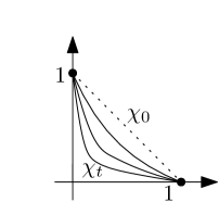
Figure 6.1. Manhattan Curves

Theorem 6.3 (Theorem D).

Following the above notations, we have for all $s\in(0,1)$

$$\left.\frac{{\rm d}^{2}\chi_{t}(s)}{{\rm d}t^{2}}\right|_{t=0}=s(s-1)\cdot||\dot{\rho}_{0}||^{2}.$$

Proof.

For a fixed $t$, ${\mathcal{C}}(\rho_{0},\rho_{t})$ can be identified as

$$\{(a,b):a,b\geq 0,a+b\neq 0,{\rm and\ }P(-a\tau_{0}-b\tau_{t})=0\}=\{(s,\chi_{t}(s)):\ P(-s\tau_{0}-\chi_{t}(s)\tau_{t})=0,s\in[0,1]\}.$$

For convenience, let us denote $\varphi_{t}(s):=-s\tau_{0}-\chi_{t}(s)\tau_{t}$. Since when $t=0,$ $\chi_{0}$ is a straight line satisfying $s+\chi_{0}(s)=1$, we have $\varphi_{0}=-\tau_{0}.$ Thus, we know $\dot{\varphi}_{0}=-\dot{\chi}_{0}\tau_{0}-\chi_{0}\dot{\tau}_{0}$ and $\ddot{\varphi}_{0}=-\ddot{\chi_{t}}\tau_{0}-2\dot{\chi}_{0}\dot{\tau}_{0}-\chi_{0}\ddot{\tau}_{0}$. By Corollary 2.13, we get

$$0=\left.\frac{{\rm d}}{{\rm d}t}P(\varphi_{t})\right|_{t=0} =\int\dot{\varphi}_{0}\,\mathrm{d}m_{\varphi_{0}}$$

$$=\int-\dot{\chi}_{0}\tau_{0}-\chi_{0}\dot{\tau}_{0}\,\mathrm{d}m_{-\tau_{0}}$$

$$=-\dot{\chi}_{0}(s)\int\tau_{0}\,\mathrm{d}m_{-\tau_{0}}-\chi_{0}(s)\int\dot{\tau}_{0}\,\mathrm{d}m_{-\tau_{0}}.$$

Since $\int\dot{\tau}_{0}\,\mathrm{d}m_{-\tau_{0}}=0$ (because $P(-\tau_{t})=0$) and $\int-\tau_{0}\,\mathrm{d}m_{-\tau_{0}}<0$, we have $\dot{\chi}_{0}(s)=0,\ \forall s\in[0,1]$. Furthermore, by taking the second derivative of pressure (as in the proof of Theorem 6.2) we get

$$0=\left.\frac{{\rm d}^{2}}{{\rm d}t^{2}}P(\varphi_{t})\right|_{t=0} ={\rm Var}(\dot{\varphi}_{0},m_{\varphi_{0}})+\int\ddot{\varphi}_{0}\,\mathrm{d}m_{\varphi_{0}}$$

$$={\rm Var}(\underset{\overset{\shortparallel}{0}}{\underbrace{-\dot{\chi}_{0}}}\tau_{0}-\chi_{0}\dot{\tau}_{0},m_{-\tau_{0}})-\int\left(\ddot{\chi_{0}}\tau_{0}+2\underset{\overset{\shortparallel}{0}}{\underbrace{\dot{\chi_{0}}}}\dot{\tau}_{0}+\chi_{0}\ddot{\tau}_{0}\right)\,\mathrm{d}m_{-\tau_{0}}$$

$$=(\chi_{0}(s))^{2}\cdot{\rm Var(}\dot{\tau}_{0},m_{-\tau_{0}})-\ddot{\chi_{0}}\int\tau_{0}\,\mathrm{d}m_{-\tau_{0}}-\chi_{0}\int\ddot{\tau}_{0}\,\mathrm{d}m_{-\tau_{0}}.$$

Notice that $P(-\tau_{t})=0,$ similarly we have

$$0=\left.\frac{{\rm d}^{2}P(-\tau_{t})}{{\rm d}t^{2}}\right|_{t=0}=-\int\ddot{\tau}_{0}\,\mathrm{d}m_{-\tau_{0}}+{\rm Var}(-\dot{\tau}_{0},m_{-\tau_{0}}).$$

Therefore, we have

$$\ddot{\chi}_{0}(s) =(\chi_{0}(s)^{2}-\chi_{0}(s))\frac{{\rm Var(}\dot{\tau}_{0},m_{-\tau_{0}})}{\int\tau_{0}\,\mathrm{d}m_{-\tau_{0}}}$$

$$=\left((1-s)^{2}-(1-s)\right))\frac{{\rm Var(}\dot{\tau}_{0},m_{-\tau_{0}})}{\int\tau_{0}\,\mathrm{d}m_{-\tau_{0}}}=(s^{2}-s)||\dot{\rho}_{0}||^{2}.$$

∎

References

- [Ahl06] Lars V. Ahlfors, Lectures on quasiconformal mappings, second ed., University Lecture Series, vol. 38, American Mathematical Society, Providence, RI, 2006, With supplemental chapters by C. J. Earle, I. Kra, M. Shishikura and J. H. Hubbard. MR 2241787
- [AK42] Warren Ambrose and Shizuo Kakutani, Structure and continuity of measurable flows, Duke Math. J. 9 (1942), 25–42. MR 0005800
- [BCLS15] Martin Bridgeman, Richard Canary, François Labourie, and Andrés Sambarino, The pressure metric for Anosov representations, Geom. Funct. Anal. 25 (2015), no. 4, 1089–1179.
- [BCS18] Martin Bridgeman, Richard Canary, and Andrés Sambarino, An introduction to pressure metrics for higher Teichmüller spaces, Ergodic Theory Dynam. Systems 38 (2018), no. 6, 2001–2035. MR 3833339
- [BI06] Luis Barreira and Godofredo Iommi, Suspension flows over countable Markov shifts, J. Stat. Phys. 124 (2006), no. 1, 207–230.
- [BS93] Christopher Bishop and Tim Steger, Representation-theoretic rigidity in PSL(2, R), Acta Mathematica 170 (1993), no. 1, 121–149.
- [Bur93] Marc Burger, Intersection, the Manhattan curve, and Patterson-Sullivan theory in rank , Internat. Math. Res. Notices (1993), no. 7, 217–225.
- [CI18] Italo Cipriano and Godofredo Iommi, Time change for flows and thermodynamic formalism, arXiv.org (2018).
- [Ham03] Ursula Hamenstädt, Length functions and parameterizations of Teichmüller space for surfaces with cusps, Ann. Acad. Sci. Fenn. Math. 28 (2003), no. 1, 75–88. MR 1976831
- [IJT15] Godofredo Iommi, Thomas Jordan, and Mike Todd, Recurrence and transience for suspension flows, Israel J. Math. 209 (2015), no. 2, 547–592.
- [JKL14] Johannes Jaerisch, Marc Kesseböhmer, and Sanaz Lamei, Induced topological pressure for countable state Markov shifts, Stoch. Dyn. 14 (2014), no. 2, 1350016–1350031.
- [Kao18] Lien-Yung Kao, Manhattan Curves for Hyperbolic Surfaces with Cusps, Ergodic Theory Dynam. Systems (2018), 1–32.
- [Kap09] Michael Kapovich, Hyperbolic manifolds and discrete groups, Modern Birkhäuser Classics, Birkhäuser Boston, Inc., Boston, MA, Boston, 2009.
- [Kem11] Tom Kempton, Thermodynamic formalism for suspension flows over countable Markov shifts, Nonlinearity 24 (2011), no. 10, 2763–2775.
- [Kim01] Inkang Kim, Marked length rigidity of rank one symmetric spaces and their product, Topology 40 (2001), no. 6, 1295–1323. MR 1867246
- [LS08] François Ledrappier and Omri Sarig, Fluctuations of ergodic sums for horocycle flows on -covers of finite volume surfaces, Discrete Contin. Dyn. Syst. 22 (2008), no. 1-2, 247–325.
- [McM08] Curtis McMullen, Thermodynamics, dimension and the Weil-Petersson metric, Invent. Math. 173 (2008), no. 2, 365–425.
- [MU01] Daniel Mauldin and Mariusz Urbański, Gibbs states on the symbolic space over an infinite alphabet, Israel J. Math. 125 (2001), no. 1, 93–130.
- [MU03] by same author, Graph directed Markov systems, Cambridge Tracts in Mathematics, vol. 148, Cambridge University Press, Cambridge, Cambridge, 2003.
- [OP04] Jean-Pierre Otal and Marc Peigné, Principe variationnel et groupes kleiniens, Duke Math. J. 125 (2004), no. 1, 15–44.
- [PPS15] Frédéric Paulin, Mark Pollicott, and Barbara Schapira, Equilibrium states in negative curvature, no. 373, Astérisque, 2015.
- [PS16] Mark Pollicott and Richard Sharp, Weil-Petersson metrics, Manhattan curves and Hausdorff dimension, Math. Z. 282 (2016), no. 3-4, 1007–1016.
- [Sar99] Omri Sarig, Thermodynamic formalism for countable Markov shifts, Ergodic Theory Dynam. Systems 19 (1999), no. 6, 1565–1593.
- [Sar01] by same author, Phase transitions for countable Markov shifts, Comm. Math. Phys. 217 (2001), no. 3, 555–577.
- [Sar03] by same author, Existence of Gibbs measures for countable Markov shifts, Proc. Amer. Math. Soc. 131 (2003), no. 6, 1751–1758 (electronic).
- [Sar09] by same author, Lecture notes on thermodynamic formalism for topological Markov shifts, 2009.
- [Sav98] Sergei V. Savchenko, Special flows constructed from countable topological Markov chains, Funktsional. Anal. i Prilozhen. 32 (1998), no. 1, 40–53, 96.
- [Sha98] Richard Sharp, The Manhattan curve and the correlation of length spectra on hyperbolic surfaces, Mathematische Zeitschrift 228 (1998), no. 4, 745–750.
- [Slo91] Zbigniew Slodkowski, Holomorphic motions and polynomial hulls, Proc. Amer. Math. Soc. 111 (1991), no. 2, 347–355. MR 1037218
- [Tuk72] Pekka Tukia, On discrete groups of the unit disk and their isomorphisms, Ann. Acad. Sci. Fenn. Ser. A I (1972), no. 504, 45 pp. (errata insert). MR 0306487
- [Tuk73] by same author, Extension of boundary homeomorphisms of discrete groups of the unit disk, Ann. Acad. Sci. Fenn. Ser. A I (1973), no. 548, 16. MR 0338358
- [Wol86] Scott Andrew Wolpert, Thurston’s Riemannian metric for Teichmüller space, Journal of Differential Geometry 23 (1986), no. 2, 143–174.