Evaluating Recurrent Neural Network Explanations

Abstract

Recently, several methods have been proposed to explain the predictions of recurrent neural networks (RNNs), in particular of LSTMs. The goal of these methods is to understand the network’s decisions by assigning to each input variable, e.g., a word, a relevance indicating to which extent it contributed to a particular prediction. In previous works, some of these methods were not yet compared to one another, or were evaluated only qualitatively. We close this gap by systematically and quantitatively comparing these methods in different settings, namely (1) a toy arithmetic task which we use as a sanity check, (2) a five-class sentiment prediction of movie reviews, and besides (3) we explore the usefulness of word relevances to build sentence-level representations. Lastly, using the method that performed best in our experiments, we show how specific linguistic phenomena such as the negation in sentiment analysis reflect in terms of relevance patterns, and how the relevance visualization can help to understand the misclassification of individual samples.

1 Introduction

Recurrent neural networks such as LSTMs Hochreiter and Schmidhuber (1997) are a standard building block for understanding and generating text data in NLP. They find usage in pure NLP applications, such as abstractive summarization Chopra et al. (2016), machine translation Bahdanau et al. (2015), textual entailment Rocktäschel et al. (2016); as well as in multi-modal tasks involving NLP, such as image captioning Karpathy and Fei-Fei (2015), visual question answering Xu and Saenko (2016) or lip reading Chung et al. (2017).

As these models become more and more widespread due to their predictive performance, there is also a need to understand why they took a particular decision, i.e., when the input is a sequence of words: which words are determinant for the final decision? This information is crucial to unmask “Clever Hans” predictors Lapuschkin et al. (2019), and to allow for transparency of the decision-making process EU-GDPR (2016).

Early works on explaining neural network predictions include Baehrens et al. (2010); Zeiler and Fergus (2014); Simonyan et al. (2014); Springenberg et al. (2015); Bach et al. (2015); Alain and Bengio (2017), with several works focusing on explaining the decisions of convolutional neural networks (CNNs) for image recognition. More recently, this topic found a growing interest within NLP, amongst others to explain the decisions of general CNN classifiers Arras et al. (2017a); Jacovi et al. (2018), and more particularly to explain the predictions of recurrent neural networks Li et al. (2016, 2017); Arras et al. (2017b); Ding et al. (2017); Murdoch et al. (2018); Poerner et al. (2018).

In this work, we focus on RNN explanation methods that are solely based on a trained neural network model and a single test data point. Thus, methods that use additional information, such as training data statistics, sampling, or are optimization-based Ribeiro et al. (2016); Lundberg and Lee (2017); Chen et al. (2018) are out of our scope. Among the methods we consider, we note that the method of Murdoch et al. (2018) was not yet compared against Arras et al. (2017b); Ding et al. (2017); and that the method of Ding et al. (2017) was validated only visually. Moreover, to the best of our knowledge, no recurrent neural network explanation method was tested so far on a toy problem where the ground truth relevance value is known.

Therefore our contributions are the following: we evaluate and compare the aforementioned methods, using two different experimental setups, thereby we assess basic properties and differences between the explanation methods. Along-the-way we purposely adapted a simple toy task, to serve as a testbed for recurrent neural networks explanations. Lastly, we explore how word relevances can be used to build sentence-level representations, and demonstrate how the relevance visualization can help to understand the (mis-)classification of selected samples w.r.t. semantic composition.

2 Explaining Recurrent Neural Network Predictions

First, let us settle some notations. We suppose given a trained recurrent neural network based model, which has learned some scalar-valued prediction function $f_{c}(\cdot)$, for each class $c$ of a classification problem. Further, we denote by $\mathbf{x}=(\boldsymbol{x_{1}},\boldsymbol{x_{2}},...,\boldsymbol{x_{T}})$ an unseen input data point, where $\boldsymbol{x_{t}}$ represents the $t$-th input vector of dimension $D$, within the input sequence $\mathbf{x}$ of length $T$. In NLP, the vectors $\boldsymbol{x_{t}}$ are typically word embeddings, and $\mathbf{x}$ may be a sentence.

Now, we are interested in methods that can explain the network’s prediction $f_{c}(\mathbf{x})$ for the input $\mathbf{x}$, and for a chosen target class $c$, by assigning a scalar relevance value to each input variable or word. This relevance is meant to quantify the variable’s or word’s importance for or against a model’s prediction towards the class $c$. We denote by $R_{x_{i}}$ (index $i$) the relevance of a single variable. This means $x_{i}$ stands for any arbitrary input variable $x_{t,d}$ representing the $d$-th dimension, $d\in\{1,...,D\}$, of an input vector $\boldsymbol{x_{t}}$. Further, we refer to $R_{\boldsymbol{x_{t}}}$ (index $t$) to designate the relevance value of an entire input vector or word $\boldsymbol{x_{t}}$. Note that, for most methods, one can obtain a word-level relevance value by simply summing up the relevances over the word embedding dimensions, i.e. $R_{\boldsymbol{x_{t}}}=\sum_{d\in\{1,...,D\}}{R_{x_{t,d}}}$ .

2.1 Gradient-based explanation

One standard approach to obtain relevances is based on partial derivatives of the prediction function: $R_{x_{i}}=\big{|}\tfrac{\partial{f_{c}}}{\partial x_{i}}(\mathbf{x})\big{|}$, or $R_{x_{i}}=\big{(}\tfrac{\partial{f_{c}}}{\partial x_{i}}(\mathbf{x})\big{)}^{2}$ Dimopoulos et al. (1995); Gevrey et al. (2003); Simonyan et al. (2014); Li et al. (2016).

In NLP this technique was employed to visualize the relevance of single input variables in RNNs for sentiment classification Li et al. (2016). We use the latter formulation of relevance and denote it as Gradient. With this definition the relevance of an entire word is simply the squared $L_{2}$-norm of the prediction function’s gradient w.r.t. the word embedding, i.e.  $R_{\boldsymbol{x_{t}}}=\|{\nabla}_{\boldsymbol{x}_{t}}\;f_{c}({\mathbf{x}})\|{{}_{2}^{2}}$ .

A slight variation of this approach uses partial derivatives multiplied by the variable’s value, i.e. $R_{x_{i}}=\tfrac{\partial{f_{c}}}{\partial x_{i}}(\mathbf{x})\cdot x_{i}$. Hence, the word relevance is a dot product between prediction function gradient and word embedding: $R_{\boldsymbol{x_{t}}}=({\nabla}_{\boldsymbol{x}_{t}}\;f_{c}({\mathbf{x}}))^{T}\,\boldsymbol{x_{t}}$  Denil et al. (2015). We refer to this variant as Gradient$\times$Input.

Both variants are general and can be applied to any neural network. They are computationally efficient and require one forward and backward pass through the net.

2.2 Occlusion-based explanation

Another method to assign relevances to single variables, or entire words, is by occluding them in the input, and tracking the difference in the network’s prediction w.r.t. a prediction on the original unmodified input Zeiler and Fergus (2014); Li et al. (2017). In computer vision the occlusion is performed by replacing an image region with a grey or zero-valued square Zeiler and Fergus (2014). In NLP word vectors, or single of its components, are replaced by zero; in the case of recurrent neural networks, the technique was applied to identify important words for sentiment analysis Li et al. (2017).

Practically, the relevance can be computed in two ways: in terms of prediction function differences, or in the case of a classification problem, using a difference of probabilities, i.e. $R_{x_{i}}=f_{c}(\mathbf{x})-f_{c}(\mathbf{x}_{|x_{i}=0})$, or $R_{x_{i}}=P_{c}(\mathbf{x})-P_{c}(\mathbf{x}_{|x_{i}=0})$, where $P_{c}(\cdot)=\tfrac{\exp f_{c}(\cdot)}{\sum_{k}{\exp f_{k}(\cdot)}}$ . We refer to the former as Occlusion${}_{\text{f-diff}}$, and to the latter as Occlusion${}_{\text{P-diff}}$. Both variants can also be used to estimate the relevance of an entire word, in this case the corresponding word embedding is set to zero in the input. This type of explanation is computationally expensive and requires $T$ forward passes through the network to determine one relevance value per word in the input sequence $\mathbf{x}$.

A slight variation of the above approach uses word omission (similarly to Kádár et al., 2017) instead of occlusion. On a morphosyntactic agreement experiment (see Poerner et al., 2018), omission was shown to deliver inferior results, therefore we consider only occlusion-based relevance.

2.3 Layer-wise relevance propagation

A general method to determine input space relevances based on a backward decomposition of the neural network prediction function is layer-wise relevance propagation (LRP) Bach et al. (2015). It was originally proposed to explain feed-forward neural networks such as convolutional neural networks Bach et al. (2015); Lapuschkin et al. (2016), and was recently extended to recurrent neural networks Arras et al. (2017b); Ding et al. (2017); Arjona-Medina et al. (2018).

LRP consists in a standard forward pass, followed by a specific backward pass which is defined for each type of layer of a neural network by dedicated propagation rules. Via this backward pass, each neuron in the network gets assigned a relevance, starting with the output neuron whose relevance is set to the prediction function’s value, i.e. to $f_{c}(\mathbf{x})$. Each LRP propagation rule redistributes iteratively, layer-by-layer, the relevance from higher-layer neurons to lower-layer neurons, and verifies a relevance conservation property. These rules were initially proposed in Bach et al. (2015) and were subsequently justified by Deep Taylor decomposition Montavon et al. (2017) for deep ReLU nets.

In practice, for a linear layer of the form $z_{j}=\sum_{i}z_{i}w_{ij}+b_{j}\;$, and given the relevances of the output neurons $R_{j}$, the input neurons’ relevances $R_{i}$ are computed through the following summation: $R_{i}=\sum_{j}\tfrac{z_{i}\cdot w_{ij}}{z_{j}\,+\,\epsilon\cdot{\text{s}ign}(z_{j})}\;\cdot R_{j}\,$, where $\epsilon$ is a stabilizer (small positive number); this rule is commonly referred as $\epsilon$-LRP or $\epsilon$-rule. With this redistribution the relevance is conserved, up to the relevance assigned to the bias and “absorbed” by the stabilizer.

Further, for an element-wise nonlinear activation layer, the output neurons’ relevances are redistributed identically onto the input neurons.

In addition to the above rules, in the case of a multiplicative layer of the form $z_{j}=z_{g}\cdot z_{s}$, Arras et al. (2017b) proposed to redistribute zero relevance to the gate (the neuron that is sigmoid activated) i.e. $R_{g}=0$, and assign all the relevance to the remaining signal neuron (which is usually tanh activated) i.e. $R_{s}=R_{j}$. We call this LRP variant LRP-all, which stands for “signal-take-all” redistribution. An alternative rule was proposed in Ding et al. (2017); Arjona-Medina et al. (2018), where the output neuron’s relevance $R_{j}$ is redistributed onto the input neurons via: $R_{g}=\tfrac{z_{g}}{z_{g}+z_{s}}R_{j}$ and $R_{s}=\tfrac{z_{s}}{z_{g}+z_{s}}R_{j}$. We refer to this variant as LRP-prop, for “proportional” redistribution. We also consider two other variants. The first one uses absolute values instead: $R_{g}=\tfrac{|z_{g}|}{|z_{g}|+|z_{s}|}R_{j}$ and $R_{s}=\tfrac{|z_{s}|}{|z_{g}|+|z_{s}|}R_{j}$, we call it LRP-abs. The second uses equal redistribution: $R_{g}=R_{s}=0.5\cdot R_{j}$ Arjona-Medina et al. (2018), we denote it as LRP-half. We further add a stabilizing term to the denominator of the LRP-prop and LRP-abs formulas, it has the form $\epsilon\cdot{\text{s}ign}(z_{g}+z_{s})$ in the first case, and simply $\epsilon$ in the latter.

Since the relevance can be computed in one forward and backward pass, the LRP method is efficient. Besides, it is general as it can be applied to any neural network made of the above layers: it was applied successfully to CNNs, LSTMs, GRUs, and QRNNs Poerner et al. (2018); Yang et al. (2018).

Method	Relevance Formulation	Redistributed Quantity ($\sum_{i}R_{x_{i}}$)	Complexity
Gradient	$R_{x_{i}}=\big{(}\tfrac{\partial{f_{c}}}{\partial x_{i}}(\mathbf{x})\big{)}^{2}$	$\|{\nabla}_{\mathbf{x}}\;f_{c}({\mathbf{x}})\|{{}_{2}^{2}}$	$\Theta(2\cdot T)$
Gradient$\times$Input	$R_{x_{i}}=\tfrac{\partial{f_{c}}}{\partial x_{i}}(\mathbf{x})\cdot x_{i}$	$({\nabla}_{\mathbf{x}}\;f_{c}({\mathbf{x}}))^{T}\,\mathbf{x}$	$\Theta(2\cdot T)$
Occlusion	$R_{x_{i}}=f_{c}(\mathbf{x})-f_{c}(\mathbf{x}_{|x_{i}=0})$	-	$\Theta(T^{2})$
LRP	backward decomposition of the neurons’ relevance	$f_{c}({\mathbf{x}})$	$\Theta(2\cdot T)$
CD	linearization of the activation functions	$f_{c}({\mathbf{x}})$	$\Theta(T^{2})$

Table 1: Overview of the considered explanation methods. The last column indicates the computational complexity to obtain one relevance value per input vector, or word, where $T$ is the length of the input sequence.

2.4 Contextual Decomposition

Another method, specific to LSTMs, is contextual decomposition (CD) Murdoch et al. (2018). It is based on a linearization of the activation functions that enables to decompose the LSTM forward pass by distinguishing between two contributions: those made by a chosen contiguous subsequence (a word or a phrase) within the input sequence $\mathbf{x}$, and those made by the remaining part of the input. This decomposition results in a final hidden state vector $h_{T}$ (see the Appendix for a full specification of the LSTM architecture) that can be rewritten as a sum of two vectors: $\beta_{T}$ and $\gamma_{T}$, where the former corresponds to the contribution from the “relevant” part of interest, and the latter stems from the “irrelevant” part. When the LSTM is followed by a linear output layer of the form $w_{c}^{T}h_{T}+b_{c}\,$ for class $c$, then the relevance of a given word (or phrase) and for the target class $c$, is given by the dot product: $w_{c}^{T}\beta_{T}$.

The method is computationally expensive as it requires $T$ forward passes through the LSTM to compute one relevance value per word. Although it was recently extended to CNNs Singh et al. (2019); Godin et al. (2018), it is yet not clear how to compute the CD relevance in other recurrent architectures, or in networks with multi-modal inputs.

See Table 1 for an overview of the explanation methods considered in the present work.

2.5 Methods not considered

Other methods to compute relevances include Integrated Gradients Sundararajan et al. (2017). It was previously compared against CD in Murdoch et al. (2018), and against the LRP variant of Arras et al. (2017b) in Poerner et al. (2018), where in both cases it was shown to deliver inferior results. Another method is DeepLIFT Shrikumar et al. (2017), however, according to its authors, DeepLIFT was not designed for multiplicative connections, and its extension to recurrent networks remains an open question. For a comparative study of explanation methods with a main focus on feed-forward nets, see Ancona et al. (2018). For a broad evaluation of explanations, including several recurrent architectures, we refer to Poerner et al. (2018). Note that the latter didn’t include the CD method of Murdoch et al. (2018), and the LRP variant of Ding et al. (2017), which we compare here.

3 Evaluating Explanations

3.1 Previous work

How to generally and objectively evaluate explanations, without resorting to ad-hoc evaluation procedures that are domain and task specific, is still active research Alishahi et al. (2019); Belinkov and Glass (2019).

In computer vision, it has become common practice to conduct a perturbation analysis Bach et al. (2015); Samek et al. (2017); Shrikumar et al. (2017); Lundberg and Lee (2017); Ancona et al. (2018); Chen et al. (2018); Morcos et al. (2018): hereby a few pixels in an image are perturbated (e.g. set to zero or blurred) according to their relevance (most relevant or least relevant pixels are perturbated first), and then the impact on the network’s prediction is measured. The higher the impact, the more accurate is the relevance.

Other studies explored in which way relevances are consistent or helpful w.r.t. human judgment Ribeiro et al. (2016); Lundberg and Lee (2017); Nguyen (2018). Some other works relied solely on the visual inspection of a few selected relevance heatmaps Li et al. (2016); Sundararajan et al. (2017); Ding et al. (2017).

In NLP, Murdoch et al. (2018) proposed to measure the correlation between word relevances obtained on an LSTM, and the word importance scores obtained from a linear Bag-of-Words. However, the latter model ignores the word ordering and context, which the LSTM can take into account, hence this type of evaluation is not adequate. Other evaluations in NLP are task specific. For example Poerner et al. (2018) use the subject-verb agreement task proposed by Linzen et al. (2016), where the goal is to predict a verb’s number, and use the relevances to verify that the most relevant word is indeed the correct subject (or a noun with the predicted number).

Other studies include an evaluation on a synthetic task: Yang et al. (2018) generated random sequences of MNIST digits and train an LSTM to predict if a sequence contains zero digits or not, and verify that the explanation indeed assigns a high relevance to the zero digits’ positions.

A further approach uses randomization of the model weights and data as sanity checks Adebayo et al. (2018) to verify that the explanations are indeed dependent on the model and data. Lastly, some evaluations are “indirect” and use relevances to solve a broader task, e.g. to build document-level representations Arras et al. (2017a), or to redistribute predicted rewards in reinforcement learning Arjona-Medina et al. (2018).

	$\rho({R_{\boldsymbol{x_{a}}}},{n_{a}})$	$\rho({R_{\boldsymbol{x_{b}}}},{n_{b}})$	$E[\frac{|{R_{\boldsymbol{x_{a}}}}|+|{R_{\boldsymbol{x_{b}}}}|}{\sum_{t}{|R_{\boldsymbol{x_{t}}}|}}]$	$E[(({R_{\boldsymbol{x_{a}}}}+{R_{\boldsymbol{x_{b}}}})-y_{\text{pred}})^{2}]$
	(in %)	(in %)	(in %)	(“MSE”)
Toy Task Addition
Gradient$\times$Input	99.960 (0.017)	99.954 (0.019)	99.68 (0.53)	24.10-4 (8.10-4)
Occlusion	99.990 (0.004)	99.990 (0.004)	99.82 (0.27)	20.10-5 (8.10-5)
LRP-prop	0.785 (3.619)	10.111 (12.362)	18.14 (4.23)	1.3 (1.0)
LRP-abs	7.002 (6.224)	12.410 (17.440)	18.01 (4.48)	1.3 (1.0)
LRP-half	29.035 (9.478)	51.460 (19.939)	54.09 (17.53)	1.1 (0.3)
LRP-all	99.995 (0.002)	99.995 (0.002)	99.95 (0.05)	2.10-6 (4.10-6)
CD	99.997 (0.002)	99.997 (0.002)	99.92 (0.06)	4.10-5 (12.10-5)
Toy Task Subtraction
Gradient$\times$Input	97.9 (1.6)	-98.8 (0.6)	98.3 (0.6)	6.10-4 (4.10-4)
Occlusion	99.0 (2.0)	-69.0 (19.1)	25.4 (16.8)	0.05 (0.08)
LRP-prop	3.1 (4.8)	-8.4 (18.9)	15.0 (2.4)	0.04 (0.02)
LRP-abs	1.2 (7.6)	-23.0 (11.1)	15.1 (1.6)	0.04 (0.002)
LRP-half	7.7 (15.3)	-28.9 (6.4)	42.3 (8.3)	0.05 (0.06)
LRP-all	98.5 (3.5)	-99.3 (1.3)	99.3 (0.6)	8.10-4 (25.10-4)
CD	-25.9 (39.1)	-50.0 (29.2)	49.4 (26.1)	0.05 (0.05)

Table 2: Statistics of the relevance w.r.t. the input numbers $n_{a}$ and $n_{b}$ and the predicted output $y_{\text{pred}}$, on toy arithmetic tasks. $\rho$ denotes the correlation and $E$ the mean. Each statistic is computed over 2500 test data points. Reported are the mean (and standard deviation in parenthesis) over 50 trained LSTM models.

3.2 Toy Arithmetic Task

As a first evaluation, we ask the following question: if we add two numbers within an input sequence, can we recover from the relevance the true input values? This amounts to consider the adding problem Hochreiter and Schmidhuber (1996), which is typically used to test the long-range capabilities of recurrent models Martens and Sutskever (2011); Le et al. (2015). We use it here to test the faithfulness of explanations. To that end, we define a setup similar to Hochreiter and Schmidhuber (1996), but without explicit markers to identify the sequence start and end, and the two numbers to be added. Our idea is that, in general, it is not clear what the ground truth relevance for a marker should be, and we want only the relevant numbers in the input sequence to get a non-zero relevance. Hence, we represent the input sequence $\mathbf{x}=(\boldsymbol{x_{1}},\boldsymbol{x_{2}},...,\boldsymbol{x_{T}})$ of length $T$, with two-dimensional input vectors as:

$$(\setcounter{MaxMatrixCols}{11}\begin{smallmatrix}0&0&0&n_{a}&0&0&0&n_{b}&0&0&0\\ n_{1}&...&n_{a-1}&0&n_{a+1}&...&n_{b-1}&0&n_{b+1}&...&n_{T}\end{smallmatrix})$$

where the non-zero entries $n_{t}$ are random real numbers, and the two relevant positions $a$ and $b$ are sampled uniformly among $\{1,...,T\}$ with $a<b$.

More specifically, we consider two tasks that can be solved by an LSTM model with a hidden layer of size one (followed by a linear output layer with no bias): the addition of signed numbers ($n_{t}$ is sampled uniformly from $[-1,-0.5]\cup[0.5,1.0]$) and the subtraction of positive numbers ($n_{t}$ is sampled uniformly from $[0.5,1.0]$). In the former case the target output $y$ is $n_{a}+n_{b}$, in the latter it is $n_{a}-n_{b}$. During training we minimize Mean Squared Error (MSE). To ensure that train/val/test sets do not overlap we use 10000 sequences with lengths $T\in\{4,...,10\}$ for training, 2500 sequences with $T\in\{11,12\}$ for validation, and 2500 sequences with $T\in\{13,14\}$ as test set. For each task we train 50 LSTMs with a validation MSE $<10^{-4}$, the resulting test MSE is $<10^{-4}$.

Then, given the model’s predicted output $y_{\text{pred}}$, we compute one relevance value $R_{\boldsymbol{x_{t}}}$ per input vector $\boldsymbol{x_{t}}$ (for the occlusion method we compute only Occlusion${}_{\text{f-diff}}$ since the task is a regression; we also don’t report Gradient results since it performs poorly). Finally, we track the correlation between the relevances and the two input numbers $n_{a}$ and $n_{b}$. We also track the portion of relevance assigned to the relevant time steps, compared to the relevance for all time steps. Lastly, we calculate the “MSE” between the relevances for the relevant positions $a$ and $b$ and the model’s output. Our results are compiled in Table 2.

Interestingly, we note that on the addition task several methods perform well and produce a relevance that correlates perfectly with the input numbers: Gradient$\times$Input, Occlusion, LRP-all and CD (they are highlighted in bold in the Table). They further assign all the relevance to the time steps $a$ and $b$ and almost no relevance to the rest of the input; and present a relevance that sum up to the predicted output. However, on subtraction, only Gradient$\times$Input and LRP-all present a correlation of near one with $n_{a}$, and of near minus one with $n_{b}$. Likewise these methods assign only relevance to the relevant positions, and redistribute the predicted output entirely onto these positions.

The main difference between our addition and subtraction tasks, is that the former requires only summing up the first dimension of the input vectors and can be solved by a Bag-of-Words approach (i.e. by ignoring the ordering of the inputs), while our subtraction task is truly sequential and requires the LSTM model to remember which number arrived first, and which number arrived second, via exploiting the gating mechanism.

Since in NLP several applications require the word ordering to be taken into account to accurately capture a sentence’s meaning (e.g. in sentiment analysis or in machine translation), our experiment, albeit being an abstract numerical task, is pertinent and can serve as a first sanity check to check whether the relevance can reflect the ordering and the value of the input vectors.

Hence we view our toy task as a minimal and unambiguous test (which besides being sequential, also exhibits a linear input-output relationship) that acts as a necessary (though not sufficient) requirement for a recurrent neural network explanation method to be trustworthy in a more complex setup, where the ground truth relevance is less clear.

For the Occlusion method, the unreliability is probably due to the fact that the neural network has always seen two “relevant” input numbers in the input sequence during training, and therefore gets confused when one of these inputs is missing at the time of the relevance computation (“out-of-sample” effect). For CD, the weakness may come from the saturation of the activations, in particular of the gates, which makes their linearization induced by the CD decomposition inaccurate.

Accuracy Change (in %)	random	Grad.	Grad.$\times$Input	LRP-prop	LRP-abs	LRP-half	LRP-all	CD	Occlusion${}_{\text{f-diff}}$	Occlusion${}_{\text{P-diff}}$
decreasing order (std$<$16)	0	35	66	15	-1	-3	97	92	96	100
increasing order (std$<$5)	0	-18	31	11	-1	3	49	36	50	100

Table 3: Average change in accuracy when removing up to 3 words per sentence, either in decreasing order of their relevance (starting with correctly classified sentences), or in increasing order of their relevance (starting with falsely classified sentences). In both cases, the relevance is computed with the true class as the target class. Results are reported proportionally to the changes for i) random removal (0% change) and ii) removal based on Occlusion${}_{\text{P-diff}}$ (100% change). For all methods, the higher the reported value the better. We boldface those methods that perform on-par with the occlusion-based relevances.

3.3 5-Class Sentiment Prediction

As a sentiment analysis dataset, we use the Stanford Sentiment Treebank Socher et al. (2013) which contains labels (very negative $--$, negative $-$, neutral $0$, positive $+$, very positive $++$) for resp. 8544/1101/2210 train/val/test sentences and their constituent phrases. As a classifier we employ the bidirectional LSTM from Li et al. (2016), which achieves 82.9% binary, resp. 46.3% five-class, accuracy on full sentences.

Perturbation Experiment. In order to evaluate the selectivity of word relevances, we perform a perturbation experiment aka “pixel-flipping“ in computer vision Bach et al. (2015); Samek et al. (2017), i.e. we remove words from the input sentences according to their relevance, and track the impact on the classification performance. A similar experiment has been conducted in previous NLP studies Arras et al. (2016); Nguyen (2018); Chen et al. (2018); and besides, such type of experiment can be seen as the input space pendant of ablation, which is commonly used to identify “relevant” intermediate neurons, e.g. in Lakretz et al. (2019). For our experiment we retain test sentences with a length $\geq$ 10 words (i.e. 1849 sentences), and remove 1, 2, and 3 words per sentence, according to their relevance obtained on the original sentence with the true class as the target class. Our results are reported in Table 3. Note that we distinguish between sentences that are initially correctly classified, and those that are initially falsely classified by the LSTM model. Further, in order to condense the “ablation” results in a single number per method, we compute the accuracy decrease (resp. increase) proportionally to two cases: i) random removal, and ii) removal according to Occlusion${}_{\text{P-diff}}$. Our idea is that random removal is the least informative approach, while Occlusion${}_{\text{P-diff}}$ is the most informative one, since the relevance for the latter is computed in a similar way to the perturbation experiment itself, i.e. by deleting words from the input and tracking the change in the classifier’s prediction. Thus, with this normalization, we expect the accuracy change (in %) to be mainly rescaled to the range $[0,100]$.

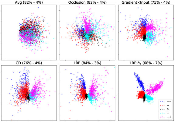
Figure 1: PCA projection of sentence-level representations built on top of word embeddings that were linearly combined using their respective relevance. Avg corresponds to simple averaging of word embeddings. For LRP ${{h}_{T}}$ the last time step hidden layer was reweighted by its relevance. In parenthesis we indicate the percentage of variance explained by the first two PCA components (those that are plotted) and by the third PCA component. The resulting representations were roughly ordered (row-wise) from less structured to more structured.

When removing words in decreasing order of their relevance, we observe that LRP-all and CD perform on-par with the occlusion-based relevance, with near 100% accuracy change, followed by Gradient$\times$Input which performs only 66%.

When removing words in increasing order of their relevance (which mainly corresponds to remove words with a negative relevance), Occlusion${}_{\text{P-diff}}$ performs best, followed by Occlusion${}_{\text{f-diff}}$ and LRP-all (both around 50%), then CD (36%). Unsurprisingly, Gradient performs worse than random, since its relevance is positive and thus low relevance is more likely to identify unimportant words for the classification (such as stop words), rather than identify words that contradict a decision, as noticed in Arras et al. (2017b). Lastly Occlusion${}_{\text{f-diff}}$ is less informative than Occlusion${}_{\text{P-diff}}$, since the former is not normalized by the classification scores for all classes.

This analysis revealed that methods such as LRP-all and CD can detect influential words supporting (resp. contradicting) a specific classification decision, although they were not tuned towards the perturbation criterion, as opposed to Occlusion (which can be seen as the brute force approach to determine the inputs the model is the most sensitive to), whereas gradient-based methods are less accurate in this respect. Remarkably LRP-all only require one forward and backward pass to provide this information.

Sentence-Level Representations. In addition to testing selectivity, we explore if the word relevance can be leveraged to build sentence-level representations that present some regularities akin word2vec vectors. For this purpose we linearly combine word embeddings using their respective relevance as weighting. For methods such as LRP and Gradient$\times$Input that deliver also relevances for single variables, we perform an element-wise weighting, i.e. we construct the sentence representation as: $\sum_{t}{R_{\boldsymbol{x_{t}}}}\odot{\boldsymbol{x_{t}}}$. For every method we report the best performing variant from previous experiments, i.e. Occlusion${}_{\text{P-diff}}$, Gradient$\times$Input, CD and LRP-all. Additionally we report simple averaging of word embeddings (we call it Avg). Further, for LRP, we consider an element-wise reweighting of the last time step hidden layer $h_{T}$ by its relevance, since LRP delivers also a relevance for each intermediate neuron (we call it LRP $h_{T}$). We also tried using $h_{T}$ directly: this gave us a visualization similar to Avg. The resulting 2D whitened PCA projections of the test set sentences are shown in Fig. 1.

Qualitatively LRP delivers the most structured representations, although for all methods the first two PCA components explain most of the data variance. Intuitively it makes also sense that the neutral sentiment is located between the positive and negative sentiments, and that the very negative and very positive sentiments depart from their lower counterparts in the same vertical direction.

The advantage of having such regularities emerging via PCA projection, is that the sentence/phrase semantics might be investigated visually, without requiring any nonlinear dimensionality reduction like t-SNE (typically used to explore the representations learned by recurrent models, e.g. in Cho et al., 2014; Li et al., 2016). Such representations might also be useful in information retrieval settings, where one could retrieve similar sentences/phrases by employing standard euclidean distance.

Composition		Predicted	Heatmap	Relevance			# samples
1.	“negated positive sentiment”	$-$		2.5 0.3	-1.4 0.5		213
2.	“amplified positive sentiment”	$++$		1.1 0.3	4.5 0.7		347
3.	“amplified negative sentiment”	$--$		0.8 0.2	4.3 0.6		173
4.	“negated amplified positive sentiment”	$-$		2.74 0.54	-0.34 0.17	-2.00 0.40	1745

Table 4: Typical heatmaps for various types of semantic compositions (indicated in first column), computed with the LRP-all method. The LSTM’s predicted class (second column) is used as the target class. The remaining columns contain the average heatmap (positive relevance is mapped to red, negative to blue, and the color intensity is normalized to the maximum absolute relevance), the corresponding word relevance mean (and std as subscript), and the number of bigrams (resp. trigrams) considered for each type of composition.

No	Predicted	Heatmap
1	$--$
1a	$+$
1b	$-$
1c	$--$
2	$++$
2a	$++$
2b	$--$
2c	$++$

Table 5: Misclassified test sentences (1 and 2), and manually constructed sentences (1a-c, 2a-c). The LSTM’s predicted class (second column) is used as the target class for the LRP-all heatmaps.

4 Interpreting Single Predictions

Next, we analyze single predictions using the same task and model as in Section 3.3, and illustrate the usefulness of relevance visualization with LRP-all, which is the method that performed well in both our previous quantitative experiments.

Semantic Composition. When dealing with real data, one typically has no ground truth relevance available. And the visual inspection of single relevance heatmaps can be counter-intuitive for two reasons: the relevance is not accurately reflecting the reasons for the classifier’s decision (the explanation method is bad), or the classifier made an error (the classifier doesn’t work as expected). In order to avoid the latter as much as possible, we automatically constructed bigram and trigram samples, which are built solely upon the classifier’s predicted class, and visualize the resulting average relevance heatmaps for different types of semantic compositions in Table 4. For more details on how these samples were constructed we refer to the Appendix, note though that in our heatmaps the negation <not>, the intensifier <very> and the sentiment words act as placeholders for words with similar meanings, since the representative heatmaps were averaged over several samples. In these heatmaps one can see that, to transform a positive sentiment into a negative one, the negation is predominantly colored as red, while the sentiment word is highlighted in blue, which intuitively makes sense since the explanation is computed towards the negative sentiment, and in this context the negation is responsible for the sentiment prediction. For sentiment intensification, we note that the amplifier gets a relevance of the same sign as the amplified word, indicating the amplifier is supporting the prediction for the considered target class, but still has less importance for the decision than the sentiment word itself (deep red colored). Both previous identified patterns also reflect consistently in the case of a negated amplified positive sentiment.

Understanding Misclassifications. Lastly, we inspect heatmaps of misclassified sentences in Table 5. In sentence 1, according to the heatmap, the classifier didn’t take the negation never into account, although it identified it correctly in sentence 1b. We postulate this is because of the strong sentiment assigned to fails that overshadowed the effect of never. In sentence 2, the classifier obviously couldn’t grasp the meaning of the words preceding must-see. If we use a negation instead, we note that it’s taken into account in the case of neither (2b), but not in the case of never (2c), which illustrates the complex dynamics involved in semantic composition, and that the classifier might also exhibit a bias towards the types of constructions it was trained on, which might then feel more “probable” or “understandable” to him.

Besides, during our experimentations, we empirically found that the LRP-all explanations are more helpful when using the classifier’s predicted class as the target class (rather than the sample’s true class), which intuitively makes sense since it’s the class the model is the most confident about. Therefore, to understand the classification of single samples, we generally recommend this setup.

5 Conclusion

In our experiments with standard LSTMs, we find that the LRP rule for multiplicative connections introduced in Arras et al. (2017b) performs consistently better than other recently proposed rules, such as the one from Ding et al. (2017). Further, our comparison using a 5-class sentiment prediction task highlighted that LRP is not equivalent to Gradient$\times$Input (as sometimes inaccurately stated in the literature, e.g. in Shrikumar et al., 2017) and is more selective than the latter, which is consistent with findings of Poerner et al. (2018). Indeed, the equivalence between Gradient$\times$Input and LRP holds only if using the $\epsilon$-rule with no stabilizer ($\epsilon=0$), and if the network contains only ReLU activations and max pooling as non-linearities Kindermans et al. (2016); Shrikumar et al. (2016). When using other LRP rules, or if the network contains other activations or product non-linearities (such as this is the case for LSTMs), then the equivalence does not hold (see Montavon et al. (2018) for a broader discussion).

Besides, we discovered that a few methods such as Occlusion Li et al. (2017) and CD Murdoch et al. (2018) are not reliable and get inconsistent results on a simple toy task using an LSTM with only one hidden unit.

In the future, we expect decomposition-based methods such as LRP to be further useful to analyze character-level models, to explore the role of single word embedding dimensions, and to discover important hidden layer neurons. Compared to attention weights (such as Bahdanau et al., 2015; Xu et al., 2015; Osman and Samek, 2019), decomposition-based explanations take into account all intermediate layers of the neural network model, and can be related to a specific class.

Appendix A Appendix

A.1 Long-Short Term Memory (LSTM) model

All LSTMs used in the present work have the following recurrence form Hochreiter and Schmidhuber (1997); Gers et al. (1999), which is also the most commonly used in the literature Greff et al. (2017):

$$\begin{split}i_{t}&=\texttt{sigm}\;\;\Big{(}W_{i}\;h_{t-1}+U_{i}\;x_{t}+b_{i}\Big{)}\\ f_{t}&=\texttt{sigm}\;\Big{(}W_{f}\;h_{t-1}+U_{f}\;x_{t}+b_{f}\Big{)}\\ o_{t}&=\texttt{sigm}\;\Big{(}W_{o}\;h_{t-1}+U_{o}\;x_{t}+b_{o}\Big{)}\\ g_{t}&=\texttt{tanh}\;\Big{(}W_{g}\;h_{t-1}+U_{g}\;x_{t}+b_{g}\Big{)}\\ c_{t}&=f_{t}\odot c_{t-1}\;+\;i_{t}\odot g_{t}\\ h_{t}&=o_{t}\odot\texttt{tanh}(c_{t})\end{split}$$

where $\mathbf{x}=(x_{1},x_{2},...,x_{T})$ is the input sequence, sigm and tanh are element-wise activations, and $\odot$ is an element-wise multiplication. The matrices $W$’s, $U$’s, and vectors $b$’s are connection weights and biases, and the initial states $h_{0}$ and $c_{0}$ are set to zero. The resulting last time step hidden vector $h_{T}$ is ultimately fed to a fully-connected linear output layer yielding a prediction vector $\boldsymbol{f}(\mathbf{x})$, with one entry ${f_{c}}(\mathbf{x})$ per class.

The bidirectional LSTM Schuster and Paliwal (1997) we use for the sentiment prediction task, is a concatenation of two separate LSTM models as described above, each of them taking a different sequence of word embedding vectors as input. One LSTM takes as input the words in their original order, as they appear in the input sentence/phrase. The other LSTM takes as input the same word sequence but in reversed order. Each of these LSTMs yields a final hidden vector, say $h^{\rightarrow}_{T}$ and $h^{\leftarrow}_{T}$. The concatenation of these two vectors is then fed to a fully-connected linear output layer, retrieving one prediction score ${f_{c}}(\mathbf{x})$ per class.

A.2 Layer-wise Relevance Propagation (LRP) implementation

We employ the code released by the authors Arras et al. (2017b) (https://github.com/ArrasL/LRP_for_LSTM), and adapt it to work with different LRP product rule variants.

In the toy task experiments, we didn’t find it necessary to add any stabilizing term for numerical stability (therefore we use $\epsilon=0$ for all LRP rules). In the sentiment analysis experiments, we use $\epsilon=0.001$ (except for the LRP-prop variant where we use $\epsilon=0.2$, we tried the following values: [0.001, 0.01, 0.1, 0.2, 0.3, 0.4, 1.0] and took the lowest one to achieve numerical stability).

A.3 Contextual Decomposition (CD) implementation

We employ the code released by the authors Murdoch et al. (2018) (https://github.com/jamie-murdoch/ContextualDecomposition), and adapt it to work with a bidirectional LSTM. We also made a slight modification w.r.t. the author’s latest available version (commit e6575aa from March 30, 2018). In particular in file sent_util.py we changed line 125 to: if i$>=$start and i$<$stop, to exclude the stop index, and call the function CD with the arguments start=k and stop=k+1 to compute the relevance of the k-th input vector, or word, in the input sequence. This consistently led to better results for the CD method in all our experiments.

A.4 Toy task setup

As an LSTM model we consider a unidirectional LSTM with a hidden layer of size one (i.e. with one memory cell $c_{t}$), followed by a linear output layer with no bias. Since the input is two-dimensional, this results in an LSTM model with 17 learnable parameters. The weights are randomly initialized with the uniform distribution $U(-1.0,1.0)$, and biases are initialized to zero. We train the model with Pytorch’s LBFGS optimizer, with an initial learning rate of 0.002, for 1000 optimizer steps, and reduce the learning rate by a factor of 0.95 if the error doesn’t decrease within 10 steps. We also clip the gradient norm to 5.0. With this setting around 1/2 of the trained models on addition and 1/3 of the models for subtraction converged to a good solution with a validation MSE $<10^{-4}$.

A.5 Semantic composition: generation of representative samples

In a first step, we build a list of words with a positive sentiment ($+$), resp. a negative sentiment ($-$), as identified by the bidirectional LSTM model. To that end, we predict the class of each word contained in the model’s vocabulary, and select for each sentiment a list of 50 words with the highest prediction scores. This way we try to ensure that the considered sentiment words are clearly identified by the model as being from the positive sentiment ($+$), resp. the negative sentiment ($-$) class.

In a second step, we build a list of negations and amplifiers. To that end, we start by considering the same lists of 39 negations and 69 amplifiers as in Strohm and Klinger (2018), from which we retain only those that are classified as neutral (class $0$) by the LSTM model, which leaves us with a list of 8 negations and 29 amplifiers. This way we discard modifiers that are biased towards a specific sentiment, since our goal is to analyze the compositional effect of modifiers.

Then, for each type of considered semantic composition (see Table 4), we generate bigrams resp. trigrams by using the previously defined lists of modifiers and sentiment words.

For compositions of type 1 (“negation of positive sentiment”), we note that among the constructed bigrams 60% are classified as negative ($-$) by the LSTM model, 26% are predicted as neutral ($0$), and for the remaining 14% of bigrams the negation is not identified correctly and the corresponding bigram is classified as positive ($+$). In order to remove negations that are ambiguous to the classifier, we retain only those negations which in at least 40% of the cases predict the bigram as negative. These negations are: [’neither’, ’never’, ’nobody’, ’none’, ’nor’]. Then we average the results over all bigrams classified as negative ($-$).

For compositions of type 2 and 3 we proceed similarly. For type 2 compositions (“amplification of positive sentiment”), we note that 29% of the constructed bigrams are classified as very positive ($++$), and for type 3 compositions (“amplification of negative sentiment”), 24% are predicted as very negative ($--$), while the remaining bigrams are of the same class as the original sentiment word (thus the amplification is not identified by the classifier). Here again we retain only unambiguous modifiers, which in at least 40% of the cases amplified the corresponding sentiment. The resulting amplifiers are: [’completely’, ’deeply’, ’entirely’, ’extremely’, ’highly’, ’insanely’, ’purely’, ’really’, ’so’, ’thoroughly’, ’utterly’, ’very’] for type 2 compositions; and [’completely’, ’entirely’, ’extremely’, ’highly’, ’really’, ’thoroughly’, ’utterly’] for type 3 compositions. Then we average the results over the corresponding bigrams which are predicted as very positive ($++$), resp. very negative ($--$).

For type 4 compositions (“negation of amplified positive sentiment”), we construct all possible trigrams with the initial lists of negations, amplifiers and positive sentiment words. We keep for the final averaging of the results only those trigrams where both the effect of the amplifier, and of the negation are correctly identified by the LSTM model. To this end we classify the corresponding bigram formed by combining the amplifier with the positive sentiment word, and keep the corresponding sample if this bigram is predicted as very positive  ($++$). Then we average the results over trigrams predicted as negative ($-$) (this amounts to finally retain 1745 trigrams).

We also tried to investigate the following composition: “negation of negative sentiment”, similarly to compositions of type 1. However, we found that only 1% of the constructed bigrams are classified as neutral ($0$), and that the remaining bigrams are classified as negative ($-$) (81%) or even very negative ($--$) (18%). This means, in most cases, negating a negative sentiment doesn’t change the classifier’s prediction, i.e. the negation is not detected by the LSTM model. Therefore we did not retain this type of composition for constructing representative heatmaps. That the impact of negation is not symmetric across different sentiments was also observed in previous works Socher et al. (2013); Li et al. (2016), and is probably due to the fact that some type of semantic compositions are more frequent than others in the training data (and more generally, in natural language) Fraenkel and Schul (2008).

References

- Adebayo et al. (2018) Julius Adebayo, Justin Gilmer, Michael Muelly, Ian Goodfellow, Moritz Hardt, and Been Kim. 2018. Sanity Checks for Saliency Maps. In Advances in Neural Information Processing Systems 31 (NIPS), pages 9505–9515.
- Alain and Bengio (2017) Guillaume Alain and Yoshua Bengio. 2017. Understanding intermediate layers using linear classifier probes. In International Conference on Learning Representations - Workshop track (ICLR).
- Alishahi et al. (2019) Afra Alishahi, Grzegorz Chrupala, and Tal Linzen. 2019. Analyzing and Interpreting Neural Networks for NLP: A Report on the First BlackboxNLP Workshop. arXiv:1904.04063. Version 1.
- Ancona et al. (2018) Marco Ancona, Enea Ceolini, Cengiz Öztireli, and Markus Gross. 2018. Towards better understanding of gradient-based attribution methods for deep neural networks. In International Conference on Learning Representations (ICLR).
- Arjona-Medina et al. (2018) Jose A. Arjona-Medina, Michael Gillhofer, Michael Widrich, Thomas Unterthiner, Johannes Brandstetter, and Sepp Hochreiter. 2018. RUDDER: Return Decomposition for Delayed Rewards. arXiv:1806.07857. Version 2.
- Arras et al. (2016) Leila Arras, Franziska Horn, Grégoire Montavon, Klaus-Robert Müller, and Wojciech Samek. 2016. Explaining Predictions of Non-Linear Classifiers in NLP. In Proceedings of the 2016 ACL Workshop on Representation Learning for NLP (Rep4NLP), pages 1–7. Association for Computational Linguistics.
- Arras et al. (2017a) Leila Arras, Franziska Horn, Grégoire Montavon, Klaus-Robert Müller, and Wojciech Samek. 2017a. ”What is relevant in a text document?”: An interpretable machine learning approach. PLoS ONE, 12(8):e0181142.
- Arras et al. (2017b) Leila Arras, Grégoire Montavon, Klaus-Robert Müller, and Wojciech Samek. 2017b. Explaining Recurrent Neural Network Predictions in Sentiment Analysis. In Proceedings of the 2017 EMNLP Workshop on Computational Approaches to Subjectivity, Sentiment and Social Media Analysis (WASSA), pages 159–168. Association for Computational Linguistics.
- Bach et al. (2015) Sebastian Bach, Alexander Binder, Grégoire Montavon, Frederick Klauschen, Klaus-Robert Müller, and Wojciech Samek. 2015. On Pixel-Wise Explanations for Non-Linear Classifier Decisions by Layer-Wise Relevance Propagation. PLoS ONE, 10(7):e0130140.
- Baehrens et al. (2010) David Baehrens, Timon Schroeter, Stefan Harmeling, Motoaki Kawanabe, Katja Hansen, and Klaus-Robert Müller. 2010. How to Explain Individual Classification Decisions. Journal of Machine Learning Research (JMLR), 11:1803–1831.
- Bahdanau et al. (2015) Dzmitry Bahdanau, Kyunghyun Cho, and Yoshua Bengio. 2015. Neural Machine Translation by Jointly Learning to Align and Translate. In International Conference on Learning Representations (ICLR).
- Belinkov and Glass (2019) Yonatan Belinkov and James Glass. 2019. Analysis Methods in Neural Language Processing: A Survey. Transactions of the Association for Computational Linguistics, 7:49–72.
- Chen et al. (2018) Jianbo Chen, Le Song, Martin Wainwright, and Michael Jordan. 2018. Learning to Explain: An Information-Theoretic Perspective on Model Interpretation. In Proceedings of the 35th International Conference on Machine Learning (ICML), pages 883–892.
- Cho et al. (2014) Kyunghyun Cho, Bart van Merrienboer, Caglar Gulcehre, Dzmitry Bahdanau, Fethi Bougares, Holger Schwenk, and Yoshua Bengio. 2014. Learning Phrase Representations using RNN Encoder-Decoder for Statistical Machine Translation. In Proceedings of the 2014 Conference on Empirical Methods in Natural Language Processing (EMNLP), pages 1724–1734. Association for Computational Linguistics.
- Chopra et al. (2016) Sumit Chopra, Michael Auli, and Alexander M. Rush. 2016. Abstractive Sentence Summarization with Attentive Recurrent Neural Networks. In Proceedings of the 2016 Conference of the North American Chapter of the Association for Computational Linguistics: Human Language Technologies (NAACL-HLT), pages 93–98. Association for Computational Linguistics.
- Chung et al. (2017) Joon Son Chung, Andrew Senior, Oriol Vinyals, and Andrew Zisserman. 2017. Lip Reading Sentences in the Wild. In IEEE Conference on Computer Vision and Pattern Recognition (CVPR), pages 3444–3453.
- Denil et al. (2015) Misha Denil, Alban Demiraj, and Nando de Freitas. 2015. Extraction of Salient Sentences from Labelled Documents. arXiv:1412.6815. Version 2.
- Dimopoulos et al. (1995) Yannis Dimopoulos, Paul Bourret, and Sovan Lek. 1995. Use of some sensitivity criteria for choosing networks with good generalization ability. Neural Processing Letters, 2(6):1–4.
- Ding et al. (2017) Yanzhuo Ding, Yang Liu, Huanbo Luan, and Maosong Sun. 2017. Visualizing and Understanding Neural Machine Translation. In Proceedings of the 55th Annual Meeting of the Association for Computational Linguistics (ACL), pages 1150–1159. Association for Computational Linguistics.
- EU-GDPR (2016) EU-GDPR. 2016. Regulation (EU) 2016/679 of the European Parliament and of the Council of 27 April 2016 on the protection of natural persons with regard to the processing of personal data and on the free movement of such data, and repealing Directive 95/46/EC (General Data Protection Regulation). Official Journal of the European Union L 119, 59:1–88.
- Fraenkel and Schul (2008) Tamar Fraenkel and Yaacov Schul. 2008. The meaning of negated adjectives. Intercultural Pragmatics, 5(4):517–540.
- Gers et al. (1999) Felix A. Gers, Jürgen Schmidhuber, and Fred Cummins. 1999. Learning to Forget: Continual Prediction with LSTM. In International Conference on Artificial Neural Networks (ICANN), volume 2, pages 850–855.
- Gevrey et al. (2003) Muriel Gevrey, Ioannis Dimopoulos, and Sovan Lek. 2003. Review and comparison of methods to study the contribution of variables in artificial neural network models. Ecological Modelling, 160(3):249–264.
- Godin et al. (2018) Fréderic Godin, Kris Demuynck, Joni Dambre, Wesley De Neve, and Thomas Demeester. 2018. Explaining Character-Aware Neural Networks for Word-Level Prediction: Do They Discover Linguistic Rules? In Proceedings of the 2018 Conference on Empirical Methods in Natural Language Processing(EMNLP), pages 3275–3284. Association for Computational Linguistics.
- Greff et al. (2017) Klaus Greff, Rupesh K. Srivastava, Jan Koutník, Bas R. Steunebrink, and Jürgen Schmidhuber. 2017. LSTM: A Search Space Odyssey. IEEE Transactions on Neural Networks and Learning Systems, 28(10):2222–2232.
- Hochreiter and Schmidhuber (1996) Sepp Hochreiter and Jürgen Schmidhuber. 1996. LSTM can Solve Hard Long Time Lag Problems. In Advances in Neural Information Processing Systems 9 (NIPS), pages 473–479.
- Hochreiter and Schmidhuber (1997) Sepp Hochreiter and Jürgen Schmidhuber. 1997. Long Short-Term Memory. Neural Computation, 9(8):1735–1780.
- Jacovi et al. (2018) Alon Jacovi, Oren Sar Shalom, and Yoav Goldberg. 2018. Understanding Convolutional Neural Networks for Text Classification. In Proceedings of the 2018 EMNLP Workshop BlackboxNLP: Analyzing and Interpreting Neural Networks for NLP, pages 56–65. Association for Computational Linguistics.
- Kádár et al. (2017) Ákos Kádár, Grzegorz Chrupala, and Afra Alishahi. 2017. Representation of Linguistic Form and Function in Recurrent Neural Networks. Computational Linguistics, 43(4):761–780.
- Karpathy and Fei-Fei (2015) Andrej Karpathy and Li Fei-Fei. 2015. Deep visual-semantic alignments for generating image descriptions. In IEEE Conference on Computer Vision and Pattern Recognition (CVPR), pages 3128–3137.
- Kindermans et al. (2016) Pieter-Jan Kindermans, Kristof Schütt, Klaus-Robert Müller, and Sven Dähne. 2016. Investigating the influence of noise and distractors on the interpretation of neural networks. arXiv:1611.07270. Version 1.
- Lakretz et al. (2019) Yair Lakretz, Germán Kruszewski, Théo Desbordes, Dieuwke Hupkes, Stanislas Dehaene, and Marco Baroni. 2019. The Emergence of Number and Syntax Units in LSTM Language Models. In Proceedings of the 2019 Conference of the North American Chapter of the Association for Computational Linguistics: Human Language Technologies (NAACL-HLT), pages 11–20. Association for Computational Linguistics.
- Landecker et al. (2013) Will Landecker, Michael D. Thomure, Luís M. A. Bettencourt, Melanie Mitchell, Garrett T. Kenyon, and Steven P. Brumby. 2013. Interpreting Individual Classifications of Hierarchical Networks. In IEEE Symposium on Computational Intelligence and Data Mining (CIDM), pages 32–38.
- Lapuschkin et al. (2016) Sebastian Lapuschkin, Alexander Binder, Grégoire Montavon, Klaus-Robert Müller, and Wojciech Samek. 2016. Analyzing Classifiers: Fisher Vectors and Deep Neural Networks. In IEEE Conference on Computer Vision and Pattern Recognition (CVPR), pages 2912–2920.
- Lapuschkin et al. (2019) Sebastian Lapuschkin, Stephan Wäldchen, Alexander Binder, Grégoire Montavon, Wojciech Samek, and Klaus-Robert Müller. 2019. Unmasking Clever Hans Predictors and Assessing What Machines Really Learn. Nature Communications, 10:1096.
- Le et al. (2015) Quoc V. Le, Navdeep Jaitly, and Geoffrey E. Hinton. 2015. A Simple Way to Initialize Recurrent Networks of Rectified Linear Units. arXiv:1504.00941. Version 2.
- Li et al. (2016) Jiwei Li, Xinlei Chen, Eduard Hovy, and Dan Jurafsky. 2016. Visualizing and Understanding Neural Models in NLP. In Proceedings of the 2016 Conference of the North American Chapter of the Association for Computational Linguistics: Human Language Technologies (NAACL-HLT), pages 681–691. Association for Computational Linguistics.
- Li et al. (2017) Jiwei Li, Will Monroe, and Dan Jurafsky. 2017. Understanding Neural Networks through Representation Erasure. arXiv:1612.08220. Version 3.
- Linzen et al. (2016) Tal Linzen, Emmanuel Dupoux, and Yoav Goldberg. 2016. Assessing the Ability of LSTMs to Learn Syntax-Sensitive Dependencies. Transactions of the Association for Computational Linguistics, 4:521–535.
- Lundberg and Lee (2017) Scott M. Lundberg and Su-In Lee. 2017. A Unified Approach to Interpreting Model Predictions. In Advances in Neural Information Processing Systems 30 (NIPS), pages 4765–4774.
- Martens and Sutskever (2011) James Martens and Ilya Sutskever. 2011. Learning Recurrent Neural Networks with Hessian-Free Optimization. In Proceedings of the 28th International Conference on Machine Learning (ICML), pages 1033–1040.
- Montavon et al. (2017) Grégoire Montavon, Sebastian Lapuschkin, Alexander Binder, Wojciech Samek, and Klaus-Robert Müller. 2017. Explaining nonlinear classification decisions with deep Taylor decomposition. Pattern Recognition, 65:211–222.
- Montavon et al. (2018) Grégoire Montavon, Wojciech Samek, and Klaus-Robert Müller. 2018. Methods for interpreting and understanding deep neural network. Digital Signal Processing, 73:1–15.
- Morcos et al. (2018) Ari S. Morcos, David G.T. Barrett, Neil C. Rabinowitz, and Matthew Botvinick. 2018. On the importance of single directions for generalization. In International Conference on Learning Representations (ICLR).
- Murdoch et al. (2018) W. James Murdoch, Peter J. Liu, and Bin Yu. 2018. Beyond Word Importance: Contextual Decomposition to Extract Interactions from LSTMs. In International Conference on Learning Representations (ICLR).
- Nguyen (2018) Dong Nguyen. 2018. Comparing Automatic and Human Evaluation of Local Explanations for Text Classification. In Proceedings of the 2018 Conference of the North American Chapter of the Association for Computational Linguistics: Human Language Technologies (NAACL-HLT), pages 1069–1078. Association for Computational Linguistics.
- Osman and Samek (2019) Ahmed Osman and Wojciech Samek. 2019. DRAU: Dual Recurrent Attention Units for Visual Question Answering. Computer Vision and Image Understanding.
- Poerner et al. (2018) Nina Poerner, Hinrich Schütze, and Benjamin Roth. 2018. Evaluating neural network explanation methods using hybrid documents and morphosyntactic agreement. In Proceedings of the 56th Annual Meeting of the Association for Computational Linguistics (ACL), pages 340–350. Association for Computational Linguistics.
- Ribeiro et al. (2016) Marco Tulio Ribeiro, Sameer Singh, and Carlos Guestrin. 2016. ”Why Should I Trust You?”: Explaining the Predictions of Any Classifier. In Proceedings of the 22nd ACM SIGKDD International Conference on Knowledge Discovery and Data Mining, pages 1135–1144.
- Rocktäschel et al. (2016) Tim Rocktäschel, Edward Grefenstette, Karl Moritz Hermann, Tomas Kocisky, and Phil Blunsom. 2016. Reasoning about Entailment with Neural Attention. In International Conference on Learning Representations (ICLR).
- Samek et al. (2017) Wojciech Samek, Alexander Binder, Grégoire Montavon, Sebastian Lapuschkin, and Klaus-Robert Müller. 2017. Evaluating the Visualization of what a Deep Neural Network has learned. IEEE Transactions on Neural Networks and Learning Systems, 28(11):2660–2673.
- Schuster and Paliwal (1997) Mike Schuster and Kuldip K. Paliwal. 1997. Bidirectional Recurrent Neural Networks. IEEE Transactions on Signal Processing, 45(11):2673–2681.
- Shrikumar et al. (2017) Avanti Shrikumar, Peyton Greenside, and Anshul Kundaje. 2017. Learning Important Features Through Propagating Activation Differences. In Proceedings of the 34th International Conference on Machine Learning (ICML), pages 3145–3153.
- Shrikumar et al. (2016) Avanti Shrikumar, Peyton Greenside, Anna Shcherbina, and Anshul Kundaje. 2016. Not Just A Black Box: Interpretable Deep Learning by Propagating Activation Differences. 1605.01713. Version 1.
- Simonyan et al. (2014) Karen Simonyan, Andrea Vedaldi, and Andrew Zisserman. 2014. Deep Inside Convolutional Networks: Visualising Image Classification Models and Saliency Maps. In International Conference on Learning Representations - Workshop track (ICLR).
- Singh et al. (2019) Chandan Singh, W. James Murdoch, and Bin Yu. 2019. Hierarchical interpretations for neural network predictions. In International Conference on Learning Representations (ICLR).
- Socher et al. (2013) Richard Socher, Alex Perelygin, Jean Y. Wu, Jason Chuang, Christopher D. Manning, Andrew Y. Ng, and Christopher Potts. 2013. Recursive Deep Models for Semantic Compositionality Over a Sentiment Treebank. In Proceedings of the 2013 Conference on Empirical Methods in Natural Language Processing (EMNLP), pages 1631–1642. Association for Computational Linguistics.
- Springenberg et al. (2015) Jost T. Springenberg, Alexey Dosovitskiy, Thomas Brox, and Martin Riedmiller. 2015. Striving for Simplicity: The All Convolutional Net. In International Conference on Learning Representations - Workshop track (ICLR).
- Strohm and Klinger (2018) Florian Strohm and Roman Klinger. 2018. An Empirical Analysis of the Role of Amplifiers, Downtoners, and Negations in Emotion Classification in Microblogs. In IEEE International Conference on Data Science and Advanced Analytics (DSAA), pages 673–681.
- Sundararajan et al. (2017) Mukund Sundararajan, Ankur Taly, and Qiqi Yan. 2017. Axiomatic Attribution for Deep Networks. In Proceedings of the 34th International Conference on Machine Learning (ICML), pages 3319–3328.
- Xu and Saenko (2016) Huijuan Xu and Kate Saenko. 2016. Ask, Attend and Answer: Exploring Question-Guided Spatial Attention for Visual Question Answering. In Computer Vision - ECCV 2016, pages 451–466.
- Xu et al. (2015) Kelvin Xu, Jimmy Ba, Ryan Kiros, Kyunghyun Cho, Aaron Courville, Ruslan Salakhutdinov, Richard Zemel, and Yoshua Bengio. 2015. Show, Attend and Tell: Neural Image Caption Generation with Visual Attention. In Proceedings of the 32nd International Conference on Machine Learning (ICML), pages 2048–2057.
- Yang et al. (2018) Yinchong Yang, Volker Tresp, Marius Wunderle, and Peter A. Fasching. 2018. Explaining Therapy Predictions with Layer-Wise Relevance Propagation in Neural Networks. In IEEE International Conference on Healthcare Informatics (ICHI), pages 152–162.
- Zeiler and Fergus (2014) Matthew D. Zeiler and Rob Fergus. 2014. Visualizing and Understanding Convolutional Networks. In Computer Vision - ECCV 2014, pages 818–833.