Structural Invertibility and Optimal Sensor Node Placement for Error and Input Reconstruction in Dynamic Systems

Abstract

Despite recent progress in our understanding of complex dynamic networks, it remains challenging to devise sufficiently accurate models to observe, control or predict the state of real systems in biology, economics or other fields. A largely overlooked fact is that these systems are typically open and receive unknown inputs from their environment. A further fundamental obstacle are structural model errors caused by insufficient or inaccurate knowledge about the quantitative interactions in the real system.

Here, we show that unknown inputs to open systems and model errors can be treated under the common framework of invertibility, which is a requirement for reconstructing these disturbances from output measurements. By exploiting the fact that invertibility can be decided from the influence graph of the system, we analyse the relationship between structural network properties and invertibility under different realistic scenarios. We show that sparsely connected scale free networks are the most difficult to invert. We introduce a new sensor node placement algorithm to select a minimum set of measurement positions in the network required for invertibility. This algorithm facilitates optimal experimental design for the reconstruction of inputs or model errors from output measurements. Our results have both fundamental and practical implications for nonlinear systems analysis, modelling and design.

I Introduction

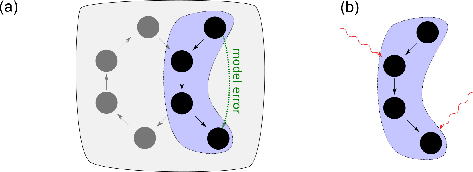
Figure 1: Schematic illustration of an open system and its environment. (a) The open system (blue shadowed region) interacts with its dynamic environment. The state (black nodes) of the open system is determined by both internal interactions and by the interactions with the (unknown) state of the environment (grey nodes). There are also systematic model errors, as indicated by a missing interaction between state variables (green dashed line). (b) Both the effects of the environment on the state of the open system and model errors can be regarded as unknown inputs.

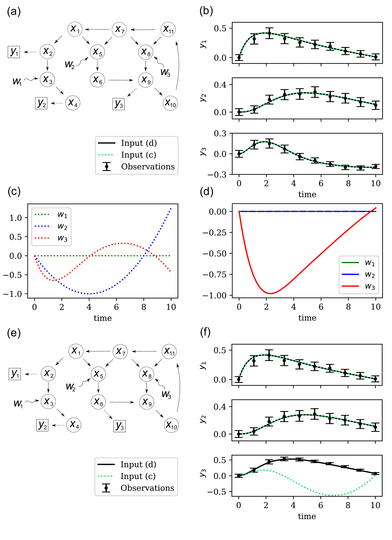
Figure 2: Invertibility of a dynamic system. (a) The influence graph represents the states ${\mbox{$x$}}=(x_{1},\ldots,x_{9})$ of a system as nodes (circles). Endogenous interactions are indicated by arrows between the states. This system receives three input signals ${\mbox{$w$}}(t)=(w_{1}(t),w_{2}(t),w_{3}(t))$ (wiggly arrows) targeting the input nodes $S=\{x_{3},x_{5},x_{8}\}$. The output ${\mbox{$y$}}(t)=(y_{1}(t),y_{2}(t),y_{3}(t))$ (squares) is given by measurements of the state variables in the sensor node set $Z=\{x_{2},x_{4},x_{9}\}$. (b) The measured output data (dots) of the open system can be explained by different input signals (c,d) causing identical outputs, as indicated by the dotted line for input (c) and by the solid line for input (d). Thus, the system is not invertible. (e) For $Z=\{x_{2},x_{4},x_{6}\}$, i.e. if the sensor for the output $y_{3}$ is moved to state $x_{6}$ instead of $x_{9}$ (compare (a)), we obtain an invertible system and the input signal in (d) is unique for the observed output in (f).

Dynamic systems in such diverse areas like physics, biology, economics or engineering are often composed of many interacting components. Developing useful and sufficiently accurate models of such complex dynamic networks having many degrees of freedom remains challenging Raue et al. (2013); Almog and Korngreen (2016); Papin et al. (2017); Tsigkinopoulou et al. (2017) despite the ever increasing size of network data sets providing the wiring diagrams of diverse systems Rossi and Ahmed (2015); Batagelj and Mrvar ; Kunegis (2013); Leskovec and Krevl .

One important challenge for modelling real dynamic networks is that they are open systems receiving inputs from their environment, see Fig. 1. These inputs need to be either known or under experimental control to fully characterise the dynamic state of the network. For example, a biological cell is a system with a certain autonomy, but at the same time is crucially dependent on signals and nutrients received from the exterior. It is practically impossible to simultaneously detect or control all signals received by a living cell in their natural environment and to measure all compounds exchanged with the extracellular space. As another example, consider a population dynamic system in a certain geographical area. The state, i.e. the population count of the different species in this area, is not only determined by the inner dynamic interactions (e.g. pray and predator relationships) between the species, but also by migration and by environmental factors. Again, for state estimation it is typically neither feasible to directly quantify all these inputs nor is it possible to ignore them. The same applies to physical, engineering, or economic systems, which will always be subject to inputs and disturbances from the environment.

If the inputs to the system cannot directly be obtained, then we might want to infer the inputs from the measurable outputs. For the biological cell, we can try to estimate the transport fluxes across the membrane and the signals received by the cell from time series of measured protein concentrations. For a population, the number of certain species will be monitored and we will try to estimate dynamic changes of birth and migration rates for other, not directly observed species. Algorithms to estimate the inputs from the outputs of systems described by ordinary differential equations (ODEs) are an ongoing research topic, see e.g. Kühl et al. (2011); Raue et al. (2012); Fonod et al. (2014); Engelhardt et al. (2016, 2017); Chakrabarty et al. (2017); Tsiantis et al. (2018). However, no such algorithm can succeed, if the output doesn’t provide sufficient information about the input. Mathematically, this means that the map from input to output is not invertible and thus, systems inversion is bound to fail.

The situation is illustrated in Fig. 2(a), where a hypothetical system is represented by an influence graph. The nodes correspond to the systems states ${\mbox{$x$}}=(x_{1},\ldots x_{11})$ and the black arrows indicate the endogenous interactions amongst them. The open system receives three input signals ${\mbox{$w$}}(t)=(w_{1}(t),w_{2}(t),w_{3}(t))$ (wiggly arrows) from its exosystem, targeting the set $S=\{x_{3},x_{5},x_{8}\}$ of three input nodes. The output signal ${\mbox{$y$}}(t)=(y_{1}(t),y_{2}(t),y_{3}(t))$ in Fig. 2(b) is formed by measuring the time course of the sensor node set $Z=\{x_{2},x_{4},x_{9}\}$, i.e.$y_{1}(t)=x_{2}(t)$, $y_{2}(t)=x_{4}(t)$ and $y_{3}(t)=x_{9}(t)$. Nonetheless, these output observations are insufficient to uniquely reconstruct the corresponding input signals. Indeed, the two different input signals (Fig. 2(c,d)) generate identical outputs (solid and dahed lines Fig. 2(b)) and both reproduce the data points with good accuracy. Thus, the system is not invertible.

The lack of invertibility can be remedied by a careful experimental design. In the example of Fig. 2, the system can be made invertible by measuring the state $y_{3}(t)=x_{6}(t)$ instead of $x_{9}(t)$, compare Fig. 2(a) and (e). As explained below, the modified output from the sensor node set $Z=\{x_{2},x_{4},x_{6}\}$ provides sufficient information to uniquely identify the input signal in Fig. 2(c) as the cause for the observed data (Fig. 2(f)). This example highlights the need for a sensor node placement algorithm for invertibility of open systems, which is one important result of this text.

Systematic model errors are another important source of potential discrepancies between measurements and model outputs. One type of model errors is caused by an incorrect influence graph, i.e. by missing or spurious interactions between the state variables (Fig. 1). Another type of model errors originates from misspecifications of the functional form or parameters of the interactions. However, both types of these endogenous model errors can effectively be treated as unknown inputs to the model system at hand, see Sec. II. As for genuine exogenous inputs, a unique reconstruction of these unknown inputs caused by endogenous model errors is again only possible if the systems model is invertible.

Controllability and observability are other important systems properties, which have attracted renewed interest from a complex systems point of view Liu et al. (2011); Cornelius et al. (2011); Liu et al. (2013); Sun and Motter (2013); Cornelius et al. (2013); Gao et al. (2014); Yan et al. (2015); Motter (2015); Liu and Barabási (2016); Summers et al. (2016); Aguirre et al. (2018); Haber et al. (2018). Structural approaches use only the influence graph Lin (1974); Liu et al. (2011, 2013); Gao et al. (2014); Motter (2015); Liu and Barabási (2016) and are therefore well suited to examine the controllability/observability properties related to topological network features. Structural controllability (observability) analysis provide binary decisions whether a system is controllable (observable) or not. Later, it was emphasised that realistic control and state estimation often require quantitative information about the network interactions and parameters of the system  Krener and Kayo (2009); Cornelius et al. (2011); Sun and Motter (2013); Cornelius et al. (2013); Yan et al. (2015); Lo Iudice et al. (2015); Summers et al. (2016); Klickstein et al. (2017); Aguirre et al. (2018); Haber et al. (2018). The underlying reason is that the specific functional form of the couplings might require huge energies for control or very sensitive measurements for state estimation. Continuous measures quantifying the degree of controllability or observability Krener and Kayo (2009); Cornelius et al. (2011); Sun and Motter (2013); Cornelius et al. (2013); Yan et al. (2015); Lo Iudice et al. (2015); Summers et al. (2016); Klickstein et al. (2017); Aguirre et al. (2018); Haber et al. (2018) were derived as alternatives to binary decisions about controllability or observability.

In contrast, the invertibility of open systems has not sufficiently been investigated in the context of large complex dynamic systems. Work in controllabity and observability of complex networks builds on older results from the control engineering literature Lin (1974), providing algebraic and graphical conditions for both traits. The situation is similar for invertibility: Theorems providing algebraic conditions for the invertibility of linear systems were already published in the 1960s R. W. Brockett and M. D. Mesarović (1965); Silverman (1969); M. Sain  and J. Massey (1969) and later extended to nonlinear systems (Hirschorn, 1979; Nijmeijer, 1982, 1986; Fliess, 1986). These algebraic conditions require a full specification of the ODE system including all the parameters. Even in the rather exceptional case, where these data are available, the numerical test of these conditions is computationally very demanding for large networks. Fortunately, invertibility is a structural property  Wey (1998); Dion et al. (2003), which can for all practical purposes be inferred from the influence graph and the input and output node sets $S$ and $Z$ (see Fig. 2). This structural invertibility condition (see Sec. III) can efficiently be tested even for very large linear or nonlinear systems with thousands of state nodes.

In this text, we add invertibility as a systems property which is essential for understanding open and incompletely known systems. As our main new contributions we

• show that unknown inputs to open systems and structural model errors can be treated under the the same conceptual framework (Sec. II);

• establish invertibility as a necessary condition for unknown input observers and input reconstruction algorithms to work (Subsec. III.7);

• provide a new recursive algebraic criterion for invertibility (Subsec. III.3);

• discover important structural network properties influencing invertibility (Sec. IV);

• provide a simple but efficient algorithm for sensor node placement to achieve structural invertibility with a minimum number of measured outputs (Sec. V).

First we show, that structural model errors in nonlinear dynamic system can be treated as unknown inputs (Sec. II). Thus, the question of whether it is possible to reconstruct model errors and unknown inputs to open systems can be treated under the common framework of invertibility. Second, we provide a novel criterion for the invertibility of linear systems, which can be used for medium sized networks up to a few hundred state nodes due to its recursive nature (Sec.  III). For large systems we exploit the structural invertibility criterion, which uses only the graph structure encoded in the interactions of the system. We will also briefly touch upon the topic of practical systems inversion, which requires careful regularisation schemes even for invertible systems. Throughout this text, we will consider three different scenarios (SC 1-3). Scenario SC 1 refers to the case, that the positions of the inputs and outputs of the system are given and that we have no opportunity to deliberately choose these positions (Sec. IV). For SC 1 we show that invertibility depends largely on the degree distribution of the influence graph and that many sparse and scale free networks tend to be non-invertible. Since many real networks show this characteristics, we assume in scenario SC 2, that the inputs are given, but the output positions can be chosen. As an important result we present a sensor node placement algorithm in Sec. V, which provides a minimum set of outputs required to uniquely reconstruct the inputs. This algorithm is also useful in scenario SC 3, where we assume that the positions of both inputs and outputs can be manipulated. We show that placing the inputs at hubs with a high out-degree can drastically increase the probability that a certain dynamic network can be made invertible, if in addition the outputs are suitably chosen, e.g. by our sensor node placement algorithm. In Sec. VI we discuss the far reaching implications of invertibility for nonlinear systems analysis and some open questions for further research.

II Open systems, unknown inputs and model errors

There are two basic reasons for discrepancies between observed time series data from a real world open system and the output of a mathematical model for the system: First, the system might receive unknown inputs Mook and Junkins (1988); Boukhobza et al. (2007); Moreno et al. (2014); Engelhardt et al. (2016); Chakrabarty et al. (2017); Engelhardt et al. (2017) from the environment, which are not covered by the model, but nevertheless influence the state and the resulting measured output. Second, there might be model errors, i.e. misspecified functional descriptions or missing interactions between internal model states or inaccurate parameter values. In this section, we define open systems with unknown inputs and then show that for ODE models, both types of error can be treated as additive unknown inputs to the model.

II.1 Open systems with unknown inputs

Consider a dynamic system $\mathcal{S}_{o}$ with time dependent state vector ${\mbox{$x$}}(t)=(x_{1}(t),\ldots,x_{N}(t))^{T}\in\mathcal{X}$. The state space $\mathcal{X}$ is either $\mathbb{R}^{N}$, a subset of it, or an $N$-manifold. A dynamic model of the open system can be formulated as a system of ordinary differential equations (ODEs)

$$\dot{{\mbox{$x$}}}(t) = {\mbox{$f$}}\left({\mbox{$x$}}(t)\right)+D{\mbox{$w$}}(t)$$ (1a)

$${\mbox{$x$}}(0) = {\mbox{$x$}}_{0}$$ (1b)

$${\mbox{$y$}}(t) = {\mbox{$c$}}\left({\mbox{$x$}}(t)\right)\,.$$ (1c)

The vector field ${\mbox{$f$}}({\mbox{$x$}})=(f_{1}({\mbox{$x$}}),\ldots,f_{N}({\mbox{$x$}}))^{T}$ represents the internal dynamic interactions between the state variables. In addition, the system receives $M$ unknown inputs, which are collected in the vector function

$${\mbox{$w$}}(t)=(w_{1}(t),\ldots,w_{M}(t))^{T}.$$ (2)

The $N\times M$ matrix $D$ describes, how the unknown input signals are distributed over the $N$ states $x$. The rows of $D$ provide information about the inputs acting on the respective state. Zero rows correspond to states which are not directly affected by model errors. As discussed below, the unknown input $w$ incorporates genuine inputs from the exterior as well as all possible types of model errors, including incorrect interactions between internal states $x$ and incorrect parameter values. The unknown input aka model error $w$ needs to be estimated from data. This would not be a problem, if the internal system state ${\mbox{$x$}}(t)$ could directly be measured. However, typically only a smaller set of $P$ scalar output signals

$${\mbox{$y$}}(t)=(y_{1}(t),\ldots,y_{P}(t))^{T}={\mbox{$c$}}\left({\mbox{$x$}}(t)\right)$$ (3)

is directly accessible to measurements. The map from the state to the output is here assumed to be given by the function ${\mbox{$c$}}\left({\mbox{$x$}}\right)$. We assume that both $f$ and $c$ satisfy a Lipschitz condition. In addition, the initial state ${\mbox{$x$}}_{0}$ needs to be specified.

It is often useful to represent systems of the form in Eq. (1) as an influence graph, see Fig. 2(a) for an example. The nodes of this directed graph correspond to the states $x_{i},\,i=1,\ldots,N$ , and the edges represent the interactions encoded by $f$. More precisely, a directed edge $x_{i}\to x_{j}$ indicates, that $\frac{\partial f_{j}}{\partial x_{i}}\neq 0$ for some $x$ in the state space $\mathcal{X}$. The state nodes targeted by unknown inputs are determined by the nonzero rows of the matrix $D$. Please note, that these input nodes are sometimes also called driver nodes, in particular in the context of control. In the special case were each unknown input component $w_{k},\,k\in\{1,2,\ldots,M\}$ affects only one state node we can choose each element $D_{ik}$ to be either zero or one and we have

$$D_{ik}\in\{0,1\}$$ (10a)

and

$$\sum_{k=1}^{M}D_{ik}=\begin{cases}1&\text{if input}\;w_{k}\;\text{affects state}\,x_{i}\\ 0&\text{otherwise}\,,\end{cases}$$ (10b)

as indicated in Fig. 2(a) by red arrows. Similarly, if the output function is given by the linear relationship ${\mbox{$c$}}\left({\mbox{$x$}}\right)=C{\mbox{$x$}}$ with the $P\times N$-matrix $C$ and if, in addition, we have $C_{ij}\in\{0,1\}$ and $\sum_{i}C_{ij}\in\{0,1\}$, we can indicate the subset of directly measured states by blue arrows. These correspond to the nonzero columns of $C$.

II.2 Model errors and unknown inputs

We now show that the unknown input function ${\mbox{$w$}}(t)$ in Eq. (1) can represent both the effect of an exterior dynamic system to our open system $\mathcal{S}_{o}$ and the effect of structural model errors in $f$, i.e. erroneous descriptions of the interactions between the internal state variables.

Let us start with a closed system $\mathcal{S}$ modelled by

$$\dot{{\mbox{$x$}}}(t)={\mbox{$f$}}\left({\mbox{$x$}}(t)\right),$$ (11)

where only the internal dynamics of the system is described, but unknown inputs are not taken into account. In reality, however, the system $\mathcal{S}$ might be embedded into a larger system (see Fig. 1) and interact also with external state variables ${\mbox{$\xi$}}(t)=(\xi_{1}(t),\ldots,\xi_{N_{\text{e}}}(t))^{T}$, which are not included in the model in Eq. (11). Instead, the joint dynamics of the system $\mathcal{S}$ and its exterior should rather be described by

$$\dot{{\mbox{$x$}}}(t) = {\mbox{$\phi$}}\left({\mbox{$x$}}(t),{\mbox{$\xi$}}(t)\right)$$ (12a)

$$\dot{{\mbox{$\xi$}}}(t) = {\mbox{$\psi$}}\left({\mbox{$x$}}(t),{\mbox{$\xi$}}(t)\right)\,.$$ (12b)

The function $\phi$ combines the effect of interactions between internal states $x$ and the effect of the external states $\xi$ on the dynamics of the internal states. The dynamics of the external system is determined by $\psi$, which is usually not known and thus difficult to include in the model. This unknown dynamics leads to the structural model error $\eta$, which can formally be defined as the discrepancy between the model in Eq. (11) and the system Eq. (12a)

$${\mbox{$\eta$}}\left({\mbox{$x$}}(t),{\mbox{$\xi$}}(t)\right):={\mbox{$\phi$}}\left({\mbox{$x$}}(t),{\mbox{$\xi$}}(t)\right)-{\mbox{$f$}}\left({\mbox{$x$}}(t)\right)\,.$$ (13)

Thus, instead of explicitly extending the simpler model Eq. (11) to the potentially complicated joint system Eq. (12), we could correct the former by adding an unknown input

$${\mbox{$\eta$}}(t):={\mbox{$\eta$}}\left({\mbox{$x$}}(t),{\mbox{$\xi$}}(t)\right)$$ (14)

to obtain

$$\dot{{\mbox{$x$}}}(t)={\mbox{$f$}}\left({\mbox{$x$}}(t)\right)+{\mbox{$\eta$}}(t)\,.$$ (15)

Replacing ${\mbox{$\eta$}}(t)=D{\mbox{$w$}}(t)$ in Eq. (15) leads to Eq. (1).

Let us illustrate the relationship between model errors and unknown inputs by a simple concrete example. Consider the following model

$$\dot{x}_{1}(t) = -0.2\,x_{1}(t)$$ (16a)

$$\dot{x}_{2}(t) = \frac{x_{1}(t)}{1+x_{4}(t)}-x_{2}(t)$$ (16b)

$$\dot{x}_{3}(t) = x_{2}(t)-x_{3}(t)$$ (16c)

$$\dot{x}_{4}(t) = x_{3}(t)-x_{4}(t)$$ (16d)

for a protein cascade Milo et al. (2002) and assume that Eq. 16c in the model is misspecified. Instead, assume that the correct description is

$$\dot{x}_{3}(t)=x_{2}(t)-\frac{x_{3}(t)}{a(t)+x_{3}(t)}\\$$ (17)

with a time dependent function $a(t)$. Thus, the degradation of $x_{3}$ is an enzyme catalysed reaction with a time dependent affinity $a(t)$, which can not be described by the mass action term in Eq. 16c. In addition, the affinity $a(t)$ is controlled by an exogenous regulatory process, which is not covered by the model in Eq. (16). The model error (compare Eq. (13)) is given by

$${\mbox{$\eta$}}(t) = \left(0,\,0,\,x_{3}(t)-\frac{x_{3}(t)}{a(t)+x_{3}(t)},\,0\right)^{T}$$

$$= \left(Dw_{1}(t)\right)^{T}$$

with $w_{1}(t)=x_{3}(t)-\frac{x_{3}(t)}{a(t)+x_{3}(t)}$ and $D=(0,0,1,0)^{T}$. If the correct relationship in Eq. (17) is unknown, we can replace Eq. (16c) by

$$\dot{x}_{3}(t)=x_{2}(t)-x_{3}(t)+w_{1}(t)\\$$ (18)

and treat $w_{1}(t)$ as an external input, which needs to be estimated from measurement data. An example for such an unknown input estimate is provided in Subsec. III.7.

III Criteria for invertibility

If the unknown input function ${\mbox{$w$}}(t)$ can uniquely be reconstructed from the output signal ${\mbox{$y$}}(t)$, we call the system invertible. An algebraic criterion to check for invertibility of a system was first derived for linear systems M. Sain  and J. Massey (1969), see Subsec. III.4 for details. An algorithm to invert the system, which terminates in the case of a non-invertibility, was also first devised for the linear case Silverman (1969), but later extended Hirschorn (1979) to nonlinear affine models of the form given in Eq. (1). Another type of results is based on differential geometric or differential algebraic criteria for the invariant control distributions Nijmeijer (1982, 1986); Fliess (1986). All these criteria involve algebraic manipulations of the systems equations, which makes them useful for smaller models, but limits their utility for large networks. In addition, the invertibility tests require a full specification of the system (Eq. (1)), including the complete functional form and the parameters of the interaction terms encoded by $f$.

Here, we state the exact mathematical definition for invertibility of dynamic systems Hirschorn (1979). Then, we provide a new recursive algorithm to check invertibility for linear systems, which might be easier to apply to systems of moderate size, in contrast to the mathematically equivalent algebraic rank condition M. Sain  and J. Massey (1969). However, for large networks, the structural invertibility algorithm has the huge advantages of scaling to large systems and of only requiring the topology of the influence graph. Invertibility is only a necessary condition and the robustness of unknown input reconstruction to measurement noise might be influenced by other factors than just the network structure. We briefly touch upon this important problem, discuss the role of regularisation and provide a simple, but illustrative example for an unknown input estimate.

III.1 Invertibility

Mathematically, invertibility means that the map from the unknown input signal $w$ to the output $y$ is injective, which can be expressed as Hirschorn (1979):

Definition 1.

The system (1) is invertible at the initial state ${\mbox{$x$}}_{0}$, if two distinct input signals ${\mbox{$w$}}(t)$ and $\tilde{{\mbox{$w$}}}(t)$ always induce two distinct outputs ${\mbox{$y$}}(t)\neq\tilde{{\mbox{$y$}}}(t)$. If the system is invertible in an open neighbourhood of ${\mbox{$x$}}_{0}$, it is called strongly invertible at ${\mbox{$x$}}_{0}$. The system is strongly invertible, if there exists a dense submanifold $\mathcal{M}$ of $\mathcal{X}$, such that the system is strongly invertible for any ${\mbox{$x$}}_{0}\in\mathcal{M}$.

For linear systems

$$\dot{{\mbox{$x$}}}(t) = A{\mbox{$x$}}(t)+D{\mbox{$w$}}(t)$$ (19a)

$${\mbox{$x$}}(0) = {\mbox{$x$}}_{0}$$ (19b)

$${\mbox{$y$}}(t) = C{\mbox{$x$}}(t)$$ (19c)

with a real $N\times N$ matrix $A$ and an $P\times N$ output matrix $C$, all the three definitions are equivalent Hirschorn (1979), since invertibility at some ${\mbox{$x$}}_{0}\in\mathbb{R}^{N}$ implies invertibility at all points in their state space $\mathcal{X}=\mathbb{R}^{N}$. Such linear systems are typically obtained as local approximations of the nonlinear model in Eq. (1), where $A$ and $C$ are given by the Jacobi matrices of $f$ and $c$, respectively, taken at a certain reference point.

For linear systems (Eq. (19)), invertibility is a global property and thus it is sufficient to consider the initial condition ${\mbox{$x$}}_{0}={\mbox{$0$}}$. Then, the input-output map $\Phi$ is given by the linear operator

$${\mbox{$y$}}(t)=\left(\Phi{\mbox{$w$}}\right)(t)=\int^{t}_{0}C\exp[{A(t-s)}]D{\mbox{$w$}}(s)\,\text{d}s\,.$$ (20)

The linear system is invertible, if this operator is one-to-one. Below, we state two different versions of an algebraic criterion to decide invertibility for linear systems. More details on the three criteria are given in the Appendix A. Here, we only motivate the structure of the algebraic criteria below: Taking successive time derivatives ${\mbox{$y$}}^{(l)}(t)$ of the output (Eq. (20)), for $l\in\{1,2,\ldots\}$

$${\mbox{$y$}}^{(l)}(t)=CA^{l}{\mbox{$x$}}(t)+\sum_{k=0}^{l-1}CA^{l-k-1}D{\mbox{$w$}}^{(k)}(t)\,,$$ (21)

and evaluating at $t=0$, we obtain the sequence of linear equations

$$\dot{{\mbox{$y$}}}(0) = CD{\mbox{$w$}}(0)$$

$$\ddot{{\mbox{$y$}}}(0) = CAD{\mbox{$w$}}(0)+CD\dot{{\mbox{$w$}}}(0)$$

$$\vdots$$

$${\mbox{$y$}}^{(l)}(0) = CA^{l-1}D{\mbox{$w$}}(0)+CA^{l-2}D\dot{{\mbox{$w$}}}(0)+$$

$$\quad\ldots+CD{\mbox{$w$}}^{(l-1)}(0)\,.$$

Invertibility implies, that we can solve these linear equations uniquely for ${\mbox{$w$}}^{(l)}(0)$ for given ${\mbox{$y$}}^{(l)}(0)$, or, equivalently, that ${\mbox{$y$}}^{(l)}(0)={\mbox{$0$}}$ implies ${\mbox{$w$}}^{(l)}(0)={\mbox{$0$}}$. Basically, the two equivalent algebraic criteria in Subsecs.  III.4 and III.3 provide conditions for unique solutions of this system.

III.2 Invertibility versus Unknown Input Observability

Let us clarify the relationship between unknown input observability and invertibility. The notion of unknown input observability is not uniquely defined in the literature. Some authors call a system unknown input observable, if the state is completely or partially observable even in the presence of unknown inputs (see e.g. Martinelli (2019)). This weaker definition does not necessarily imply that the unknown input itself can be reconstructed. Other authors define unknown input observability in the stricter sense that both the systems state as well as the unknown input can be inferred from the outputs Boukhobza et al. (2007).

Invertibility or structural invertibility ensures, that the unknown input can uniquely be reconstructed from the output. It does not necessarily imply that the system state can simultaneously be observed Boukhobza et al. (2007). Only if the initial state ${\mbox{$x$}}_{0}$ is known, then invertibility is not only necessary but also sufficient for simultaneous state and input observability.

It is only recently, that a general algorithm for testing the weaker form of unknown input observability of nonlinear systems exists Martinelli (2019). This algorithm is based on symbolic computation and thus restricted to very small systems with only a few state variables.

III.3 Recursive Algebraic Criterion for Invertibility of Linear Systems

For the first version of the algebraic criterion we define a sequence of block matrices

$$R_{l}:=\left[(CD)(CAD)\ldots(CA^{l}D)\right]\,,\quad l\in\mathbb{N}_{0}\,,$$ (22)

which appear in the derivatives of the output (Eq. (21)). Each matrix $R_{l}$ in the sequence has $P$ rows and $(l+1)M$ columns. Recall, that $P$ was the number of measurement signals and $M$ the number of unknown inputs. For each matrix $R_{l}$ in the sequence, the null space is defined as

$$\ker R_{l}=\left\{{\mbox{$v$}}\in\mathbb{R}^{(l+1)M}\left|\,R_{l}{\mbox{$v$}}={\mbox{$0$}}\right.\right\}\,,\quad l\in\mathbb{N}_{0}\,.$$ (23)

In addition, we recursively define the following sets

$$K_{0} := \ker R_{0}\backslash\{0\}$$

$$K_{l} := \ker R_{l}\cap\left(\mathbb{R}^{M}\times K_{l-1}\right)\,.$$

Here, “$\times$” indicates the cartesian product of two sets. Now we can state the invertibility criterion: The linear system in Eq. (19) is invertible, if and only if $K_{l}$ is the empty set $\emptyset$ for some $l\leq N-1$.

To apply this criterion we have to calculate the null spaces of all $R_{l}$ and then iteratively to evaluate the sequence of sets $K_{l}$, starting from $l=0$. The iteration terminates if $K_{l}=\emptyset$ for some $l\leq N-1$, indicating invertibility. If no such $l$ can be found, the system is not invertible.

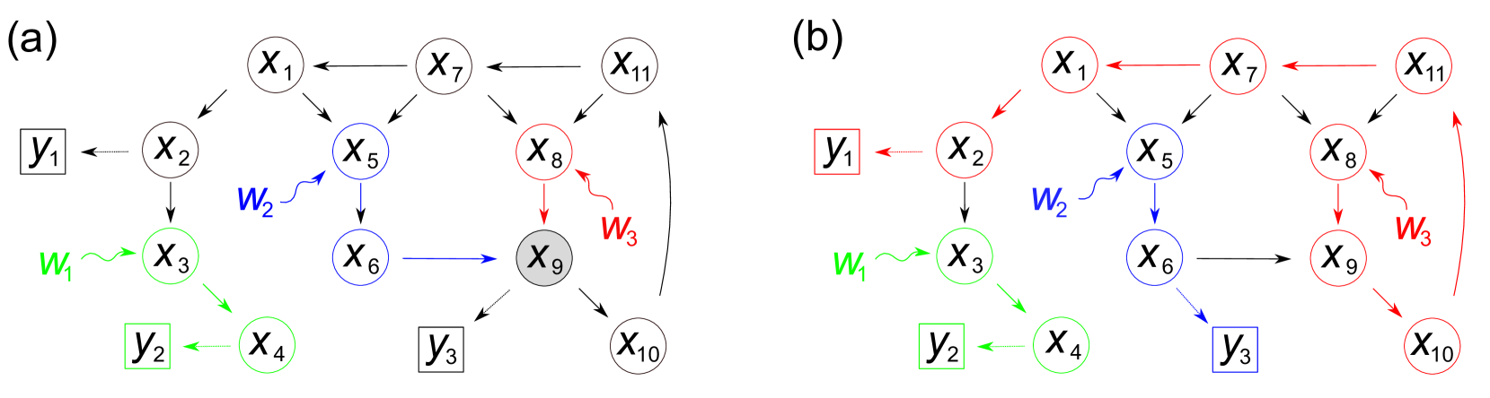
Figure 3: The graphical condition for invertibility. (a) The system represented by the influence graph with input node set $S=\{x_{3},x_{5},x_{8}\}$ is non-invertible, if the output measurements ${\mbox{$y$}}=(y_{1},y_{2},y_{3})$ (squares) are placed at the sensor node set $Z=\{x_{2},x_{4},x_{9}\}$. The only possible paths from the input nodes $x_{5}$ and $x_{8}$ to any of the outputs (here $y_{3}$) collide at $x_{9}$. (b) The same graph with the same input nodes $S$ as in (a), but with outputs ${\mbox{$y$}}=(y_{1},y_{2},y_{3})$ (squares) placed at $Z=\{x_{2},x_{4},x_{6}\}$ (i.e. $x_{6}$ replaces the sensor node $x_{9}$ in (a)) is invertible. There is a family $\Pi=\{{\color[rgb]{0,1,0}w_{1}\rightsquigarrow x_{3}\rightarrow x_{4}\rightarrow y_{2}},\,{\color[rgb]{0,0,1}w_{2}\rightsquigarrow x_{5}\rightarrow x_{6}\rightarrow y_{3}},\,{\color[rgb]{1,0,0}w_{3}\rightsquigarrow x_{8}\rightarrow x_{9}\rightarrow x_{10}\rightarrow x_{11}\rightarrow x_{7}\rightarrow x_{1}\rightarrow x_{2}\rightarrow y_{1}}\}$ of three non intersecting (node disjoint) paths joining each input with one output.

III.4 Rank Condition for Invertibility of Linear Systems

The iterative criterion above is equivalent to the following algebraic rank condition proofed by Sain and Massey M. Sain  and J. Massey (1969): Consider the sequence of matrices

$$Q_{l}:=\begin{bmatrix}CD&CAD&\dots&CA^{l}D\\ 0&CD&\dots&CA^{l-1}D\\ \vdots&&\ddots&\vdots\\ 0&\dots&&CD\end{bmatrix}$$ (24)

for $l\in\mathbb{N}_{0}$. The linear system in Eq. (19) is invertible, if and only if

$$\text{rank}\,Q_{N-1}-\text{rank}\,Q_{N-2}=M\,.$$ (25)

As before, $N$ is the number of states in the system and $M$ the number of inputs. Thus, the criterion requires to compute the rank of two matrices. The size of these matrices increases quadratically with the number of states $N$ in the system. Such rank computations can be very memory intensive for large networks with many nodes.

It is worthwhile remarking on an interesting property of invertibility. For an invertible system, the null space of the operator $\Phi$ is zero dimensional, containing as its single element the zero input ${\mbox{$w$}}(t)\equiv{\mbox{$0$}}$. For a non-invertible system, the null space of $\Phi$ is always infinite dimensional (see Lemma 1 in the Appendix). This means that for non-invertible systems there are infinitely many independent inputs which cannot be distinguished from each other. This shows, that there is no such thing like “nearly invertible”. Thus, any algorithm attempting to infer the inputs for the outputs is bound to fail without further assumptions about the inputs. Assumptions like smoothness and sparsity of the input signals can be encoded into these inversion algorithms by using suitable regularisation schemes Engelhardt et al. (2016) or Bayesian priors Engelhardt et al. (2017). However, even these additional smoothness and sparsity assumptions restricting the domain of the input-output map are not always sufficient for invertibility Engelhardt et al. (2016).

III.5 Graphical Criterion for Linear and Nonlinear Systems

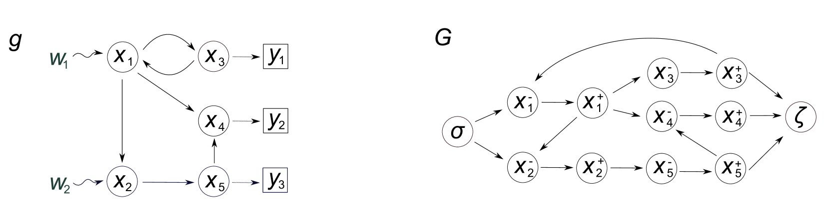
Figure 4: An example for the structural invertibility algorithm counting the number of node-disjoint paths connecting the input node set $S=\{x_{1},x_{2}\}$ with the output node set $Z=\{x_{3},x_{4},x_{5}\}$. The influence graph $g$ is transformed into the graph $G$ by replicating each of the state nodes $x_{1},\ldots,x_{5}$ to $x_{1}^{+},\ldots,x_{5}^{+}$ and $x_{1}^{-},\ldots,x_{5}^{-}$, thereby separating the ingoing and outgoing edges. A family of node-disjoint paths in $g$ corresponds to a family of edge-disjoint paths in $G$. Then, an additional source node $\sigma$ is connected to the inputs and an additional sink node $\zeta$ to the outputs and edge weights of $1$ are added to $G$. The maximum flow from $\sigma$ to $\zeta$ corresponds to the number of node-disjoint paths from $S$ to $Z$ in g.

The quite intricate algebraic conditions can be replaced by a simple graphical criterion Dion et al. (2003), see Fig. 3. Recall, that in the influence graph $g$ each state variable $x_{i}$ is represented as a node and the edges are determined by the adjacency matrix $A$: For each $A_{ji}\neq 0$ draw an directed edge $i\to j$. Now assume, that the columns of the input matrix consist only of a subset of $M$ canonical basis vectors ${\mbox{$e$}}_{k}\in\mathbb{R}^{N}$. Thus $D_{ik}\in\{0,1\}$ with $\sum_{k}D_{ik}\in\{0,1\}$. Then, the nonzero rows of $D$ indicate the states receiving an input signal. Denote these $M$ input nodes as

$$S=\{s_{1},\ldots,s_{M}\}\subseteq\{x_{1},\ldots,x_{N}\}\,.$$ (26)

Similarly, we assume that the output matrix $C$ has only $P$ rows which are a subset of the canonical basis of $\mathbb{R}^{P}$ and thus $C_{ji}\in\{0,1\}$ with $\sum_{j}C_{ji}\in\{0,1\}$. Then, the nonzero columns of $C$ indicate the output or sensor nodes

$$Z=\{z_{1},\ldots,z_{P}\}\subseteq\{x_{1},\ldots,x_{N}\}\,,$$ (27)

i.e. the state nodes for which direct measurements are available.

Now, the graphical criterion can be stated as follows: The linear system in Eq. (19) is structurally invertible, if and only if there is a family $\Pi$ of $M$ directed paths in the influence graph $g$ fulfilling the following conditions

1. Each path in $\Pi$ starts in $S$ and terminates in $Z$.

2. All paths of $\Pi$ are pairwise node-disjoint.

In the following, we will call the triplet $(S,g,Z)$ consisting of the influence graph $g$, the input node set $S$ and the output node set $Z$ invertible, if the structural invertibility criterion is fulfilled.

To put it differently: There must be a family $\Pi$ of directed paths in $g$ connecting each input node in $S$ with an output node in $Z$ and no two paths in the family intersect at any node of the influence graph. If no such family of node-disjoint paths exists, the systems is structurally non-invertible. For the example graphs in Fig. 2(a,b), this path condition is illustrated in Fig. 3(a,b) for the non-invertible (a) and invertible case (b), respectively. Obviously, a system with fewer output nodes than input nodes is never invertible.

This intuitive graphical condition implies, that only the structure of the influence graph and the position of the inputs and outputs, i.e. only the patterns of nonzero entries in the systems matrices $A$, $D$, and $C$, are relevant for invertibility Dion et al. (2003). Indeed, structural invertibility and algebraic invertibility coincide up to pathological cases, where the graphical condition could indicate structural invertibility, whereas none of the algebraic conditions would be fulfilled due to an exact cancellation of numerical terms. These pathological conditions are irrelevant in practice, since any arbitrarily small numerical perturbation of one of the nonzero terms in the systems matrices would repair invertibility. Or, in mathematical language: The set of systems matrices $A$, $D$, and $C$, for which the graphical and the algebraic conditions give contradictory results is a set of measure zero. The situation is completely analogous to the structural and algebraic controllability or observability conditions Lin (1974); Dion et al. (2003); Liu et al. (2011, 2013).

The structural invertibility condition was extended to nonlinear systems of the form in Eq. (1), see Wey (1998) for details. This means, that we can replace the matrix $A$ by the Jacobi matrix of $f$ and the output matrix $C$ by the Jacobi matrix of $c$ at some point of the state space $\mathcal{X}$ to obtain the systems graph and the output node set $Z$. Thus, the structural properties of the linearisation of Eq. (1) are also sufficient to detect the invertibility of a nonlinear system. There is one subtlety for nonlinear systems: The structural invertibility condition does not imply regularity of the system, which is relevant for feedback systems, see Wey (1998) for further details.

III.6 Structural Invertibility Algorithm

The graphical criterion for (structural) invertibility requires to count the number of node-disjoint paths connecting the input nodes $S$ with the output nodes $Z$. Counting all these paths in a combinatorial manner is not feasible for larger systems. Thanks to the Max-Flow-Min-Cut-Theorem Menger (1927); Dion et al. (2003); B. Korte and J. Vygen (2018), the graphical node disjoint path counting problem can be reformulated as flow problem, which can efficiently be solved.

As an initial step of the algorithm, the influence graph $g$ is transformed to a corresponding flow graph $G$ by copying each node $i$ to separate the ingoing and outgoing edges (see Fig. 4). Now, a familiy $\Pi$ of node-disjoint paths in the original graph $g$ corresponds to a family of edge-disjoint paths in $G$. In a second step, an additional source node $\sigma$ is connected to each of the input nodes and an additional sink node $\zeta$ is connected to each of the output nodes. If each edge in the resulting graph $G$ is assigned a weight of $1$, the maximum flow from source $\sigma$ to sink $\zeta$ in $G$ equals the number of edge-disjoint paths from source to sink, and thus the number of node-disjoint paths from $S$ to $Z$ in the original graph $g$. In our implementation we use the Goldberg-Tarjan algorithm A. Goldberg (1988) to efficiently compute the maximum flow. Several alternative algorithms exist in the combinatorial optimisation literature, see e.g. B. Korte and J. Vygen (2018).

To analyse the computational complexity of the structural invertibility algorithm, let $N$ and $E$ be the number of nodes and edges in the original graph $g$. As before, we denote the number of input nodes by $M$ and the number of sensor nodes by $P$. In directed graphs the number of edges is limited by $E\leq N^{2}$. For large networks we can assume $M\approx P<<N$. To create the flow graph $G$, $n=2N+2$ nodes and $e=N+E+M+P$ edges are created. On $G$ we use the Goldberg-Tarjan algorithm with running time scaling like $\mathcal{O}(n^{2}\sqrt{e})$ to compute the maximum flow. All together we find that the structurally invertibility algorithm has a running time of $\mathcal{O}(N^{3})$. Please note that there are even more efficient optimised versions of the Goldberg-Tarjan algorithm with better running time B. Korte and J. Vygen (2018), but for all our purposes the standard version was sufficient.

Our implementation is based on the python networkx package. On a single node of an Intel® Xeon® Processor E5-2690 v2 we need an average time of $0.15\pm 0.03$ seconds for a network with $N=10^{3}$ nodes and $2.4\pm 0.4$ seconds for $N=10^{4}$ nodes to decide structural invertibility.

III.7 Practical invertibility and robustness

Invertibility (or structural invertibility) is a necessary condition for the unique reconstruction of unknown inputs ${\mbox{$w$}}(t)$ from outputs ${\mbox{$y$}}(t)$. If the input-output map $\Phi$ defined by the general system in Eq. (1) is invertible, the operator equation

$${\mbox{$y$}}=\Phi{\mbox{$w$}}$$ (28)

for given ${\mbox{$y$}}={\mbox{$y$}}(t)$ has a unique solution ${\mbox{$w$}}(t)$ and the inverse operator $\Phi^{-1}$ exists.

In reality, we have to reconstruct the unknown input $w$ from measured output data ${\mbox{$y$}}^{\text{data}}$, which will always be subject to measurement errors and noise. Therefore, the data based estimate $\hat{{\mbox{$w$}}}=\Phi^{-1}{\mbox{$y$}}^{\text{data}}$ will differ from the true input ${\mbox{$w$}}=\Phi^{-1}{\mbox{$y$}}$. For a discontinuous inverse operator $\Phi^{-1}$, the difference between $\hat{{\mbox{$w$}}}$ and $w$ can be drastic. Unfortunately, the inverse operator of the general nonlinear system Eq. (1) is not continuous. Thus, estimating the unknown input from real data remains an ill posed problem Engl et al. (2000); G. Nakamura and R. Potthast (2015), even if the system is invertible and $\Phi^{-1}$ exists.

The underlying reason for the discontinuity of the inverse input-output operator $\Phi^{-1}$ of the linear system (Eq. (19)) is a well known theorem from the theory of inverse problems (see e.g. Engl et al. (2000); G. Nakamura and R. Potthast (2015)): Linear compact operators with an infinite dimensional range cannot have a continuous inverse. The linear input-output operator Eq. (20) corresponding to the linear system in Eq. (19) is an integral operator and thus it is compact and has infinite range, as shown in the Appendix (Theorem 1). For nonlinear operators, a similar theorem states that completely-continous operators with infinite range cannot have a continuous inverse. This indicates, that the inverse of the nonlinear system Eq. (1) cannot be continuous.

The degree of discontinuity of the inverse to the linear compact operator in Eq. (20) can be quantified by means of the singular value decomposition (SVD). Since $\Phi$ has an infinite dimensional range, its SVD is an infinite series. The infinite series $(\sigma_{k}),\,k=1,2,\ldots$ of singular values is usually ordered by decreasing magnitude ($\sigma_{k+1}\geq\sigma_{k})$. The smaller singular values determine the response of $\Phi^{-1}$ to high frequency components of ${\mbox{$y$}}^{\text{data}}$ and are thus responsible for the discontinuity of the inverse. Thus, it is in principle possible to quantify the degree of discontinuity by the speed of decay of the sequence $(\sigma_{k})$. The problem in Eq. (28) is considered to be mildly ill-posed, if the sequence of singular value $(\sigma_{k})$ decays at most with polynomial speed, whereas it is called severely ill-posed, if $(\sigma_{k})$ decays faster than any polynomial Engl et al. (2000). However, this approach is not straightforward to implement, because it requires computing the spectrum of the gramian operator $\Phi^{*}\,\Phi$, where $\Phi^{*}$ is the adjoint of Eq. (20). In addition, it is not yet clear whether the SVD can also be useful for the inverse nonlinear input-output operator corresponding to nonlinear system Eq. (1), possibly after a suitable linearisation. This is certainly beyond the scope of this text and we leave this as an interesting direction for further research.

Please note, that the situation for invertibility is different from that of controllability or observability  Krener and Kayo (2009); Cornelius et al. (2011); Sun and Motter (2013); Cornelius et al. (2013); Yan et al. (2015); Summers et al. (2016); Aguirre et al. (2018); Haber et al. (2018), where the corresponding gramian matrices correspond to operators with finite dimensional range. Consequently, there is a smallest singular value which can be used as the condition number characterising the degree of controllability or observability, respectiveley.

Regularisation of Unknown Inputs

There are several algorithms for estimating the unknown input $w$ from measurement data, ranging from feedback controllers via modifications of the nonlinear Kalman filter to moving horizon estimation  Kühl et al. (2011); Raue et al. (2012); Fonod et al. (2014); Engelhardt et al. (2016, 2017); Chakrabarty et al. (2017); Tsiantis et al. (2018). We can not discuss all these approaches here, but it is instructive to briefly discuss a simple version of the optimisation based approach, where an error functional $J[{\mbox{$w$}}]$ is minimised with respect to ${\mbox{$w$}}(t)$. This leads to the following optimal control problem

$$\text{minimize}\,J[{\mbox{$w$}}]=d[{\mbox{$y$}}^{\text{data}},{\mbox{$y$}}]+R[{\mbox{$w$}}]$$ (29)

subject to

$$\dot{{\mbox{$x$}}}(t)={\mbox{$f$}}({\mbox{$x$}}(t))+{\mbox{$w$}}(t)$$

$${\mbox{$y$}}(t)={\mbox{$c$}}({\mbox{$x$}})\,.$$

Here, $d$ quantifies the fit of the corrected model output $y$ to the data ${\mbox{$y$}}^{\text{data}}$. A typical choice is the squared error

$$d[{\mbox{$y$}}^{\text{data}},{\mbox{$y$}}] = \frac{1}{T}\sum_{i=1}^{P}\int_{0}^{T}\left(y_{i}^{\text{data}}(t)-y_{i}(t)\right)^{2}\text{d}t$$

$$\approx \frac{1}{n}\sum_{i=1}^{P}\sum_{k=1}^{n}\left(y_{i}^{\text{data}}(t_{k})-y_{i}(t_{k})\right)^{2}\,.$$

Usually, one has discrete time measurements ${\mbox{$y$}}^{\text{data}}(t_{k})$ at time points $t_{k}\in[0,T],\,k=0,1,\ldots,n$ and the discrete time squared error in the second row is used instead of the integral. If the components of the output function have very different magnitudes, it is often also useful to use a weighted squared error. In addition, for zero mean gaussian measurement noise ${\mbox{$y$}}^{\text{data}}-{\mbox{$y$}}$, the squared error corresponds to the log-likelihood function G. Nakamura and R. Potthast (2015).

The regularisation term $R[{\mbox{$w$}}]$ in Eq. (29) can be chosen to penalise overly complex input functions ${\mbox{$w$}}(t)$. The regularisation parameter $\alpha\geq 0$ provides a way of balancing the data fit ($d$) with the complexity of the estimated function ${\mbox{$w$}}(t)$. There are several ways to select the regularisation parameter. One useful idea is known as the discrepancy principle G. Nakamura and R. Potthast (2015), where the regulation parameter is chosen such that the data error $d$ is approximatl y equal to the level of measurement noise.

Even for invertible systems the regularisation is necessary, because the unregularised least squares fit ($\alpha=0$) will be very sensitive to measurement errors, again a symptom of the discontinuity of the inverse input-output operator $\Phi^{-1}$ corresponding to Eq. (1). Typical choices for the regularisation function are

$$R[{\mbox{$w$}}]=\frac{1}{T}\sum_{i=1}^{p}\int_{0}^{T}w_{i}^{2}(t)\text{d}t\,,$$

which penalises the squared 2-norm of the unknown input $w$ or

$$R[{\mbox{$w$}}]=\frac{1}{T}\int_{0}^{T}\dot{w}^{2}_{i}(t)\text{d}t\,,$$ (30)

which penalises the norm of the first derivative $\dot{{\mbox{$w$}}}$. These two examples are known as Tikhonov regularisation in function spaces G. Nakamura and R. Potthast (2015). For linear operators like the Eq. (20), the effect of the regularisation is to suppress the effect of small singular values. There are many more possible choices for regularisation terms, e.g. sparsity promoting regularisation Engelhardt et al. (2016). Often, regularisation terms are also chosen to render the optimisation problem convex, which avoids problems with local minima Abarbanel (2013).

Example for an unknown input estimate

In our computational experiments we found the regularisation of the derivative as in Eq. $\eqref{eq:reg_deriv}$ to yield good results for the case of additive measurement noise, where ${\mbox{$y$}}^{\text{data}}-{\mbox{$y$}}$ is a zero mean stochastic disturbance of the output measurement. This is illustrated in Fig. 5 for the model of a protein cascade Milo et al. (2002)

$$\dot{x}_{1}(t) =-0.2\,x_{1}(t)+w_{1}(t)$$ (31)

$$\dot{x}_{2}(t) =\frac{x_{1}(t)}{1+x_{4}(t)}-x_{2}(t)$$

$$\dot{x}_{3}(t) =x_{2}(t)-x_{3}(t)+w_{2}(t)$$

$$\dot{x}_{4}(t) =x_{3}(t)-x_{4}(t)\,,$$

with known initial value

$${\mbox{$x$}}_{0}=(1,0.5,0.5,0.1)^{T}\,.$$ (32)

We generated synthetic data by solving the system of ODEs for a given input function ${\mbox{$w$}}(t)$ acting on the input nodes $S=\{x_{1},x_{3}\}$ and adding gaussian noise to the output, see Fig. 5(a,b). We then tried to recover the input from the noisy output data by solving the regularised optimal control problem in Eqs. (29) and (30). If the measurement nodes are $Z=\{x_{3},x_{4}\}$, the measured output data can accurately be fitted (Fig. 5(b)), but the recovered inputs 5(c) do not correspond to the true inputs. The reason is that the system with the output nodes $Z=\{x_{3},x_{4}\}$ is not structurally invertible. For the sensor node set $Z=\{x_{2},x_{4}\}$, the system is structurally invertible and the solution of the optimal control problem (Eqs. (29) and (30)) provides a reconstruction of the inputs from the noisy measurements, see Fig. 5(d-f). In particular, the magnitude of the estimate for $w_{1}$ is very small and differs from the true unknown input $w_{1}=0$ only due to transient effects of the numerics and measurement noise.

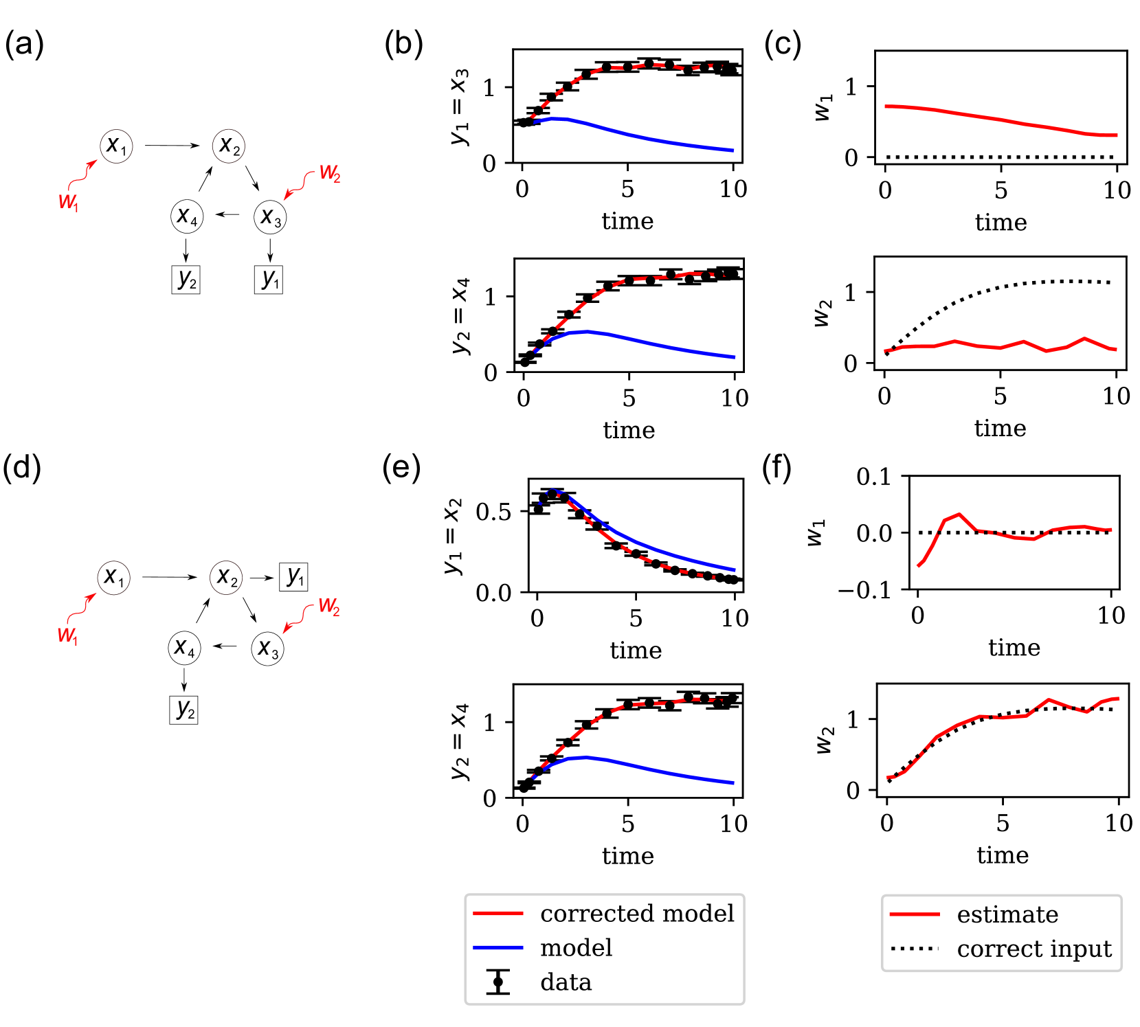
Figure 5: Estimation of unknown inputs to a simple protein cascade. (a) The influence graph of the system in Eq. (31) with input nodes $S=\{x_{1},x_{3}\}$ and output nodes $y_{1}=x_{3}$ and $y_{2}=x_{4}$. (b) The model output for the system without unknown inputs (blue) can not reproduce the observed data (dots with error bars for measurement noise). Solving the regularised optimisation problem (see Eqs. (29) and (30)) provides accurate fits to the data (red line). (c) However, the estimates of the unknown inputs (red lines) are incorrect (dashed lines indicate the true inputs), because the system is not structurally invertible. (d) The system is structurally invertible, if $y_{1}=x_{2}$ and $y_{2}=x_{4}$ are measured. (e,f) The fit to the measurements in (e) is now sufficient to estimate the unknown inputs in (f). Please note also the different scale of the plots for in (c) and (f). All values are understood in arbitrary units.

This simple example illustrates again the importance of structural invertibility as a prerequisite for systems inversion. As discussed above, the accuracy of the estimates can vary with the degree of continuity of the inverse input-output operators, which itself depends on the functional form and on the specific parameters of the ODE. However, structural invertibility is a necessary requirement to estimate unknown inputs or model errors. Therefore, we will focus on structural aspects of invertibility in the remainder of this text.

IV Structural Invertibility of Complex Networks

It is natural to ask whether certain network properties affect structural invertibility. It has been shown previously, that important systems properties including controllability Liu et al. (2011), observability Liu et al. (2013) or target controllability Gao et al. (2014) are related to network structure, see Motter (2015); Liu and Barabási (2016) for reviews.

In this section we will explore the invertibility of large simulated and real networks using the very efficient structural invertibility algorithm from Subsec. III.6. To mimick scenario SC 1, where we have no influence on the choice of the input and output nodes, we will first use a uniform random sampling scheme for the selection of both node sets. Later, we will investigate the effect of hubs on invertibility and study the preferential selection of hubs as input or output nodes.

IV.1 Invertibility of random and scale free networks under uniform sampling (scenario SC 1)

Figure 6: The structural invertibility of (a) Erdős-Rényi random graphs and (b) scale free networks (power law exponent $\gamma=2.4$) depends on the average node degree $\bar{d}$. For each data point, an ensemble of $100$ networks with $N=10^{3}$ nodes was simulated and disjoint sets of $M=P$ input and output nodes were chosen by uniform random sampling. Each network was tested for structural invertibility and the fraction $\rho$ of invertible networks in the ensemble was recorded. For large networks with many nodes $N\to\infty$ and fixed average degree $\bar{d}$, the function $\rho(\bar{d},N,M)$ asymptotically approaches $\rho(\bar{d},M)$. We found empirically that $N=10^{3}$ is a good approximation for this asymptotic regime.

Intuitively, a densely connected network allows to find many node-disjoint paths connecting the input node set $S$ to the output node set $Z$. Thus, for a set of randomly selected input nodes $S$ and a disjoint set of randomly selected output nodes $Z$, the chance for invertibility should increase with the average degree $\bar{d}$ of the network $g$.

To test this hypothesis, we simulated graphs with $N=10^{3}$ nodes using either Erdős-Rényi random graphs P. Erdős and A. Rényi (1960) or scale-free networks A.-L. Barabási and R. Albert (1999); Goh et al. (2001) with varying average degree $\bar{d}$. Throughout these simulations, we used $M=P$, i.e. the same number of input and output nodes. For a given graph $g$, we first sampled a set $S$ of $M$ input nodes uniformly at random and then randomly sampled the set $Z$ of $P$ output nodes from the remaining nodes, such that the input and output node sets are disjoint: $S\cap Z=\emptyset$. We will refer to this sampling scheme for inputs and outputs as uniform random sampling, which simulates scenario SC 1. Then, we used the structural invertibility algorithm to check whether the resulting network represents the influence graph of an invertible or a non-invertible system (Eq. (20)). To estimate the probability $\rho=\rho(\bar{d},N,M)$, that a graph with $N$ nodes, $M=P$ inputs and outputs and average degree $\bar{d}$ is invertible under this random scheme, we sampled $100$ triples of $(S,g,Z)$ of different graphs and input/output node sets and counted the relative frequency of structurally invertible systems represented by these graphs.

As can be seen in Fig. 6(a), the probability of invertibility for Erdős-Rényi random graphs increases indeed monotonously with the average degree $\bar{d}$. For small $\bar{d}$, almost no graph is invertible, whereas for large $\bar{d}$ almost all graphs are invertible. These two regimes are separated by a transition zone, where some networks are invertible and others are not. In this transition zone, invertibility depends on the specific characteristics of the random graph and the average degree is not sufficient to decide about invertibility. For more inputs and outputs (increasing $M=P$), the transition zone moves towards higher $\bar{d}$. This is plausible, because a family of $M=P$ node disjoint paths $\Pi$ connecting the input and the output sets $S$ and $Z$ cannot be found in sparse networks with a small overall number of paths. We found empirically, that for $M=P$ the function $\rho=\rho(\bar{d},N,M)$ attains an asymptotic limit $\rho(\bar{d},M)$ for large networks with a given average degree ($N\to\infty$ and $\bar{d}$ fixed).

Scale-free networks offer another network topology induced by a power law degree distribution $P(k)\propto k^{-\gamma}$ that has been observed to be the underlying structure of many real networks (A.-L. Barabási and R. Albert, 1999; Goh et al., 2001). Scale-free networks have a tendency for a few highly connected hubs and many weakly connected satellites. The effect of this heterogeneity is not immediately obvious: On the one hand, the hubs act as bottlenecks, that shrink the chance of finding node-disjoint paths. On the other hand, the diameter of scale-free networks is much smaller than the diameter of Erdős-Rényi random graphs R. Cohen and S. Havlin (2003); hence paths are shorter and might possibly find their way to the output set $Z$, before they intersect.

The python networkx package was used to do the simulations. For the Erdős-Rényi graphs $g=g(N,p)$ we used fast_gnp_random_graph. We implemented the static model from Goh et al. (2001) to generate scale-free graphs $g=g(\bar{d},N,\gamma)$. Here, $N$ is the node number, $p$ the probability, that an edge in the Erdős-Rényi graph exists, $\bar{d}$ is the average degree and $\gamma$ the exponent in the power law degree distribution. As before we drew $100$ graphs, distributed $M=P$ input and output nodes uniformly over each graph, and took $\rho$ as the fraction of structural invertible graphs. For a given number of inputs and outputs, the transition zone for scale free networks (see Fig. 6(b)) is broader in comparison to Erdős-Rényi systems. In scale free networks, increasing the number of inputs and outputs has a more drastic effect on diminishing the chance for invertibility, as can be seen from the larger gaps between the different curves in Fig. 6(b) compared to Fig. 6(a). For the same average degree $\bar{d}$, one is less likely to sample an invertible combination of inputs and outputs in a scale free network than in a homogenous Erdős-Rényi random graph. Thus, under the uniform random placement scheme (scenario SC 1) of inputs and outputs, hubs are typically detrimental for invertibility.

IV.2 The role of the degree distribution

Figure 7: Effect of the degree distribution on invertibility under the uniform random scheme. (a) The fraction of structural invertible input-output configurations for the E.coli metabolic network (black dots) is compared to an ensemble of scale free random networks with the same power law exponent $\gamma=2.61$ and the same average degree $\bar{d}=11.17$. (b,c) The out-degree versus the in-degree for the E.coli metabolic network (b) and a typical scale free network (c).

To explore the effect of the degree distribution on invertibility, we compared the scale free E.coli metabolic network Schellenberger et al. (2010) to an ensemble of simulated scale free networks. The E.coli metabolic network has an estimated power law exponent of $\gamma=2.61$ and an average degree of $\bar{d}=11.17$. We used the static model and the same parameters to simulate the ensemble of 100 scale free networks. We selected 100 input and output node sets for the E.coli network using uniform random sampling (scenario SC 1) and computed the fraction $\rho$ of invertible systems as a function of the number $M=P$ of in- and outputs. The uniform random sampling scheme was also applied to each of the 100 simulated scale free graphs. Intriguingly, we found that the probability for invertibility $\rho$ is higher in the simulated networks than in the E.coli metabolic network, see Fig. 7(a). In addition, we performed a degree-preserving randomization (rand-Degree) S. Maslov  and K. Sneppen (2002) to all networks (E.coli and simulated) and found that this doesn’t change $\rho$, up to small sampling deviations (see next Subsec. IV.3). In this degree-preserving randomization, the in-degree $d_{\text{in}}$ (number of incoming edges) and the out-degree $d_{\text{out}}$ (number of outgoing edges) of each node is preserved, but the nodes which link to each other are randomly selected.

In Fig. 7(b,c) we have plotted $d_{\text{out}}$ versus $d_{\text{in}}$ for the E.coli metabolic network (b) and a typical simulated scale free network (c). It can be seen, that the E.coli network has many more high degree nodes with a large difference $d_{\text{out}}-d_{\text{in}}$ between out- and in-degree. This asymmetry is by construction much smaller in the simulated networks. These results indicate, that the joint distribution of in- and out-degrees $P(d_{in},d_{out})$ largely determines the probability of finding an invertible system under the uniform input-output sampling scheme (scenario SC 1).

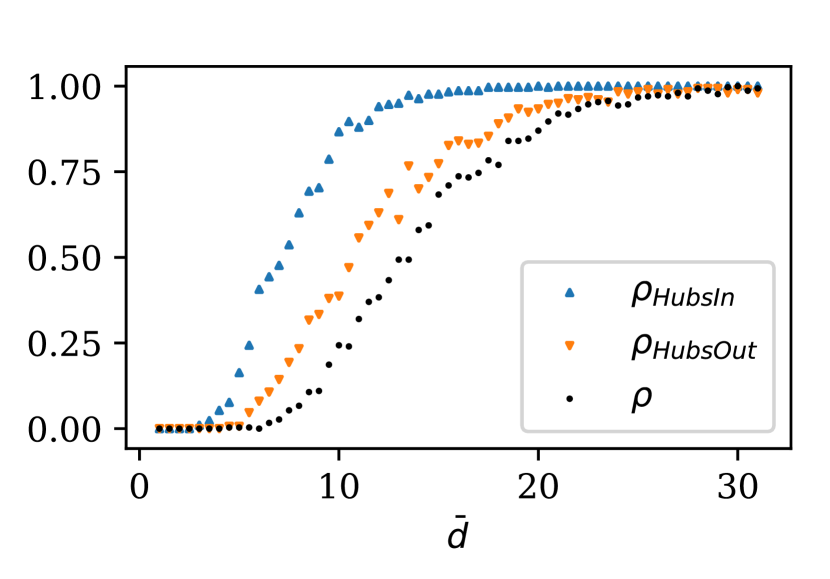
Figure 8: Preferential sampling of hubs as input nodes (blue) or output nodes (orange) for an ensemble of $300$ scale free networks ($N=500$, $M=P=10$, $\gamma=2.4$). The blue triangles show the fraction of invertible networks, when the $M=10$ nodes with highest degree are chosen as input nodes and the $P=10$ output nodes are sampled uniformly from the remaining $N-M=490$ nodes. Conversely, for the orange symbols, the $P=10$ nodes with highest degree were chosen as outputs and the inputs were uniformly sampled from the remaining $N-P=490$ nodes. The black dots were obtained for the same uniform random scheme as in Fig. 6, were both inputs and outputs were sampled uniformly (scenario SC 1).

To further explore the role of hubs in networks with a more symmetric assignment of in- and output nodes, we modified the uniform random scheme. Instead of uniform sampling (see IV.1), we now ranked all the state nodes according to their degree and selected the $M$ nodes with the highest degree as input set $S$. The $P=M$ output nodes $Z$ were again uniformly sampled from the remaining nodes. As can be seen from Fig. 8, this preferred selection of hub nodes as inputs can drastically increase the probability of invertibility in scale free networks. A less drastic improvement can also be observed, when the high degree nodes are used as outputs and then the input nodes are uniformly sampled.

IV.3 Invertibility of real networks under uniform sampling of inputs and outputs (scenario SC 1)

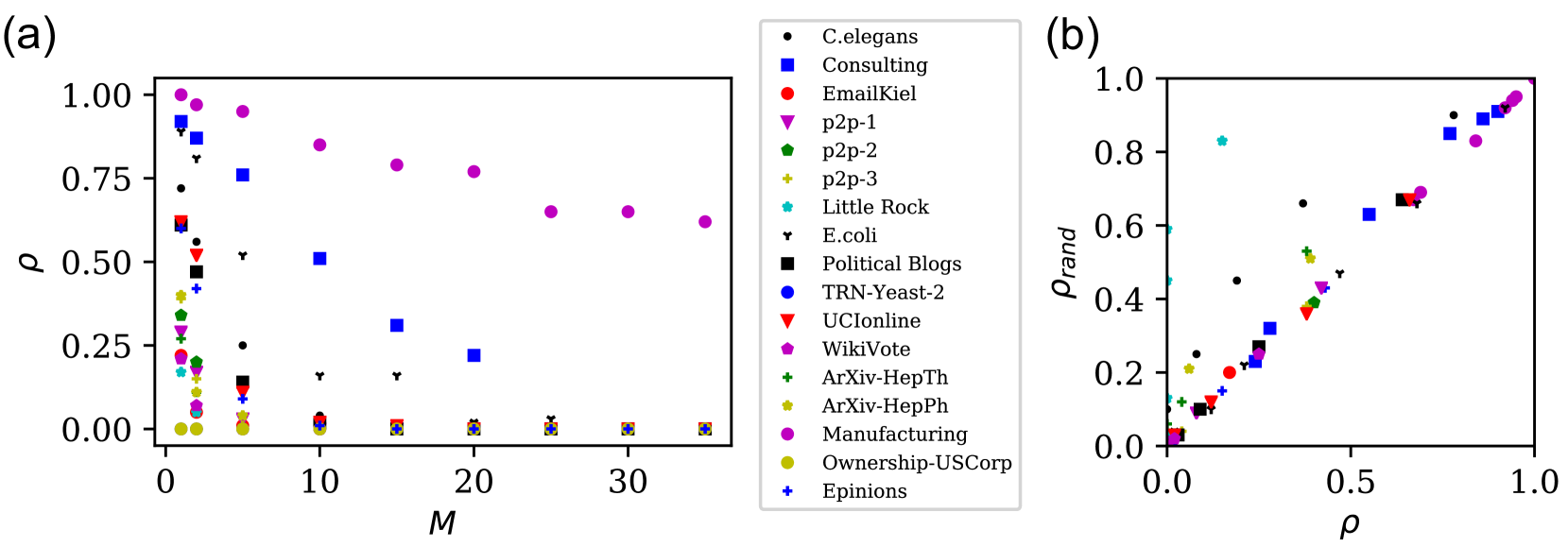
Figure 9: Structural invertibility of real networks. (a) The probability of invertibility under the random scheme. For each network in Table 1, the disjoint sets of $M=P$ in- and ouput nodes were obtained by uniform random sampling (scenario SC 1). This was repeated $100$ times for each $M$ and the fraction $\rho$ of structural invertible graphs was estimated. (b) Comparison of $\rho$ from (a) to the probability of invertibility after a degree-preserving randomization ($\rho_{\text{rand}}$). Note that some of the symbols are exactly masking each other. In this randomisation, the in- and out-degree of each node is preserved and the nodes linked to each other are randomly selected S. Maslov  and K. Sneppen (2002).

Name	$N$	$|\mathcal{E}|$	$\bar{d}$	Scalefree	$\gamma$	Brief Description	Database
Regulatory
TRN-Yeast-2 Milo et al. (2002)	688	1079	3.14	True	2.29	Transcriptional regulatory network of S.cerevisiae	Uri Alon Lab Alon
Ownership-USCorp Norlen et al. (2002)	7253	6726	1.85	True	2.45	Ownership network of US corporations	Pajek Batagelj and Mrvar
Trust
WikiVote Leskovec et al. (2009)	7115	103689	29.13	False		Who-vote-whom network of Wikipedia users	snap Stanford Leskovec and Krevl
Epinions Richardson et al. (2003)	75888	508837	13.41	True	1.73	Who-trust-whom network of Epinions.com users	snap Stanford Leskovec and Krevl
Food Web
Little Rock Martinez (1991)	183	2494	27.26	False		Food Web in Little Rock lake	Mount Sinai Ma’ayan Laboratory Department of Pharmacology and Therapeutics
Metabolic
E.coli Schellenberger et al. (2010)	1039	5802	11.17	True	2.61	Network of the metabolic reactions of the E. coli bacteria	BiGG BiGG Models
Neuronal
C.elegans D. J. Watts and S. H. Strogatz (1998)	297	2345	15.79	True	2.15	Neural network of C.elegans	Network Repository Rossi and Ahmed (2015)
Citation
ArXiv-HepTh Leskovec et al. (2005)	27770	352807	25.41	False		Citation networks in HEP-TH category of Arxiv	snap Stanford Leskovec and Krevl
ArXiv-HepPh Leskovec et al. (2005)	34546	421578	24.41	False		Citation networks in HEP-PH category of Arxiv	snap Stanford Leskovec and Krevl
WWW
Political blogs L. A. Adamic and N. Glance (2005)	1224	19025	31.09	True	1.04	Hyperlinks between weblogs on US politics	Moreno Datasets (a)
Internet
p2p-1 Leskovec et al. (2007)	10876	39994	7.36	False		Gnutella peer-to-peer file sharing network	snap Stanford Leskovec and Krevl
p2p-2 Leskovec et al. (2007)	8846	31839	7.2	False		Same as above (at different time)	snap Stanford Leskovec and Krevl
p2p-3 Leskovec et al. (2007)	8717	31525	7.2	False		Same as above (at different time)	snap Stanford Leskovec and Krevl
Social Communication
UCIonline T. Opsahl and P. Panzarasa (2009)	1899	20296	21.38	True	1.33	Online message network of students at UC, Irvine	Opsahl Datasets (b)
EmailKiel Ebel et al. (2002)	57194	103731	3.63	True	1.77	Email network of traffic data collected at University of Kiel, Germany	Barabasi Liu et al. (2013)
Intraorganizational
Manufacturing R. L. Cross and A. Parker (2004)	77	2228	3.14	False		Social network from a manufacturing company	Opsahl Datasets (b)
Consulting R. L. Cross and A. Parker (2004)	46	879	38.22	False		Social network from a consulting company	Opsahl Datasets (b)

Table 1: A compilation of networks from various fields, also examined by other authors (Liu et al. (2013)). Here $N$ is the number of nodes and $|\mathcal{E}|$ the number of edges. The column “Scale free” indicates whether the degree distribution shows a power law and if so, the power law exponent $\gamma$ was computed.

In addition to the E.coli metabolic network, we tested a compilation of real networks (Table 1) for invertibility under the uniform input-output sampling scheme (scenario SC 1). Again, we estimated the probability of invertibility $\rho$ as a function of the number of in- and output nodes $M=P$, see Fig. 9(a). Here, we observe a ranking with the (not scale-free) Intraorganizational networks on top, with the highest chance for structural invertibility, followed by the (scale-free) biological E.coli and C.elegans networks. Many of the remaining networks are much larger, with $N>10^{5}$ nodes, and have a higher average degree. Nevertheless, the chance to find a structural invertible in- and output configuration under the uniform sampling scheme is vanishingly small already for $M=P\approx 5$ for many real networks in this compilation. Thus, in these networks, it is typically difficult to reconstruct unknown inputs or model errors, if the outputs nodes are chosen randomly and the inputs can not be selected. These results are robust under a degree-preserving randomisation S. Maslov  and K. Sneppen (2002), where the nodes linked to each other are randomly selected, but the in-degree $d_{\text{in}}$ and out-degree $d_{\text{out}}$ of each node is preserved (Fig. 9(b)).

To summarise, we find that invertibility under the uniform random scheme (scenario SC 1) depends mainly on the joint distribution of in- and out-degree. Dense and homogeneous networks tend to be invertible, while sparse and scale-free networks provide a smaller chance to reconstruct structural model errors and hidden inputs. As emphasised by the results for real networks, more efficient ways to select sensor nodes or inputs are required. The positive effects of the preferential selection of hubs, either as inputs or outputs, hint at possible ways to improve the chance for invertibility under different scenarios, where only outputs (SC 2) or both input and output (SC 3) nodes can deliberately be selected.

V Sensor node placement for invertibility

Whilst the uniform random scheme (scenario SC 1) provides some insights into the effects of network properties on invertibility, it is not a very efficient strategy to randomly place the sensor nodes over the network.

A second, more realistic scenario (SC 2) is the following: Assume, we have observed a systematic discrepancy between the output measurements and the model and we want to infer the unknown inputs (or model errors). Assume further, that the input node set $S$ is given, either from domain knowledge about the respective system or from educated guessing about possible positions for input signals or model errors. However, the system might not be invertible with the current output node set. Typically, we know which states could in principle be measured and we can define a maximum set $Z_{0}$ of potential sensor nodes. If the resulting system with the maximum output set $Z_{0}$ is invertible, one can start the acquisition of time series data and feed them into one of the algorithms Kühl et al. (2011); Raue et al. (2012); Fonod et al. (2014); Engelhardt et al. (2016, 2017); Chakrabarty et al. (2017); Tsiantis et al. (2018). to infer the input. This approach, though straightforward, would potentially be wasteful or even impractical. In domains like biology or economics, measurements might in principle be possible, but costly or take a great deal of time. Thus, a more feasible approach is to reduce this excessive effort by selecting a minimum set of sensor nodes from the maximum set $Z_{0}$.

A similar sensor node placement problem for state observability Boukhobza et al. (2007); Liu et al. (2013) has been investigated before. In this section, we present a very simple but efficient greedy algorithm to select a minimum set of sensor nodes for invertibility for a given fixed set of input nodes (scenario SC 2). This algorithm can drastically improve the chances for invertibility, as we will demonstrate by comparing to uniform random sampling for scenario SC 1. Finally, we will also investigate a third scenario SC 3, where the input nodes can also be selected.

V.1 Sensor node placement algorithm

Let us formalise the scenario SC 2 motivated above: The influence graph $g$ for dynamic system (19) including a set $S$ of $M$ potential input nodes is assumed to be given. In addition, we have an initial maximum set

$$Z_{0}=\{z_{1},\ldots,z_{P_{0}}\}\subseteq\{x_{1},\ldots,x_{N}\}$$ (33)

of $P_{0}$ potential output or sensor nodes. Thus, $Z_{0}$ incorporates all systems states which could potentially be monitored. If the system with $S$ as given input set and $Z_{0}$ as maximum output set is not invertible, then there is no way to reconstruct the inputs from the outputs. However, if invertibility is ensured for $Z_{0}$, then we want to reduce this maximum set to a smaller, potentially minimal subset $Z^{*}\subseteq Z_{0}$ with $P^{*}$ outputs, which is still invertible, given the inputs $S$.

From the structural invertibility theorem (see Subsec. III.5) we know that the smallest output set has at least as many nodes as the input set. Thus, we will always have $P^{*}\geq M$. For small sets $Z_{0}$, it might be possible to try all $\binom{P_{0}}{M}$ possible subsets of $M$ nodes from the maximum set $Z_{0}$. However, this brute force strategy becomes quickly infeasible, if $P_{0}$ is large. Reducing $P_{0}$ from the beginning is usually also not an option, since the maximum sensor node set $Z_{0}$ needs to provide an invertible system, which might not be the case for small sets.

A practical solution is given by a simple greedy algorithm, which assumes that the triple $(S,g,Z_{0})$ containing the maximum node set $Z_{0}$ is invertible. To initialise the algorithm, we assume that the nodes are in some random order in $Z_{0}$. In the first iteration, we select the first node $z$ from $Z_{0}$ and try to delete it, but only if $(S,g,Z_{0}\setminus z)$ with $P_{0}-1$ sensor nodes is still invertible. If not, we keep $z$ in the node set $Z_{1}:=Z_{0}$, i.e. we reject the deletion of this node. Otherwise we delete the node by setting $Z_{1}:=Z_{0}\setminus z$. In any case, we continue and try to delete a different node, say the next node in $Z_{1}$. We proceed in this way until we have a sensor node set $Z_{k}$ with $P_{k}=M$ output nodes and set $Z^{*}=Z_{k}$. This algorithm takes at most $P_{0}-M$ steps. Note, that the greedy algorithm will always find a minimum node set with the minimum number $P^{*}=M$ of sensor nodes, provided $(S,g,Z_{0})$ with the initial node set $Z_{0}$ is invertible.

In Fig. 10 we present an example for a network with $N=1000$ nodes and $M=100$ uniformly sampled input nodes. All other nodes were included in the maximum output set $Z_{0}$, i.e. $P_{0}=900$. The algorithm takes $598$ iterations to find a minimum node set $Z^{*}$ with $P^{*}=100$. The number of iterations can be reduced by replacing the random removal of output nodes by a more selective satellite-deletion strategy. By ranking the nodes in $Z_{0}$ according to their degree and selectively removing nodes with low degree shrinks the (invertible) output set much faster than random deletion. Reversing the order of the ranking, i.e. trying to selectively delete hubs from the set of sensor nodes results in more rejections and thus more iterations (Fig. 10). This is consistent with the results from (Fig. 8), were we found that preferential selection of high degree output nodes improves the chance for invertibility. Please note, that the greedy algorithm is usually fast enough for most purposes, even without ranking the nodes. This analyses merely serves to better understand the role of hubs as inputs or outputs.

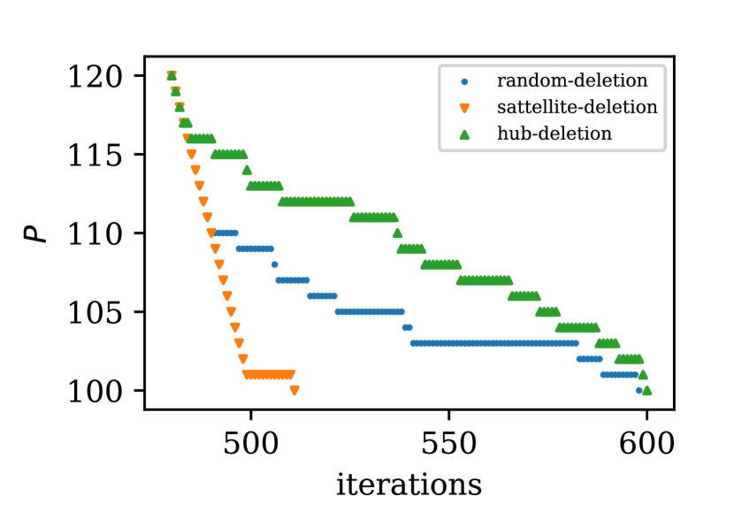
Figure 10: The greedy algorithm for optimal sensor node selection for invertibility applied to a network with $N=1000$ state nodes, and $M=100$ randomly distributed inputs. From the remaining $900$ nodes, the maximum output set $Z_{0}$ with $P_{0}=700$ potential sensor nodes was randomly chosen. The plot compares the number of sensor nodes $P$ versus the number of iterations of the greedy algorithm for random-, satellite-, and hub-deletion strategies.

V.2 Application to real networks

The sensor node placement algorithm can only be successful, if the maximum sensor node set $Z_{0}$ (together with the given input node set) yields an invertible system. Larger $Z_{0}$, i.e. a larger number $P_{0}$ of potentially measurable outputs, will obviously increase the chances for invertibility and thus also the chance to find a minimum sensor node set $Z^{*}$ of cardinality $P^{*}=M$. Apart from directly measuring all possible nodes, the largest possible nontrivial sensor node set $Z_{0}$ is given by the $N-M$ nodes which are not input nodes. We used this $Z_{0}$ with $P_{0}=N-M$ to check the compendium of real networks (Table 1) for invertibility.

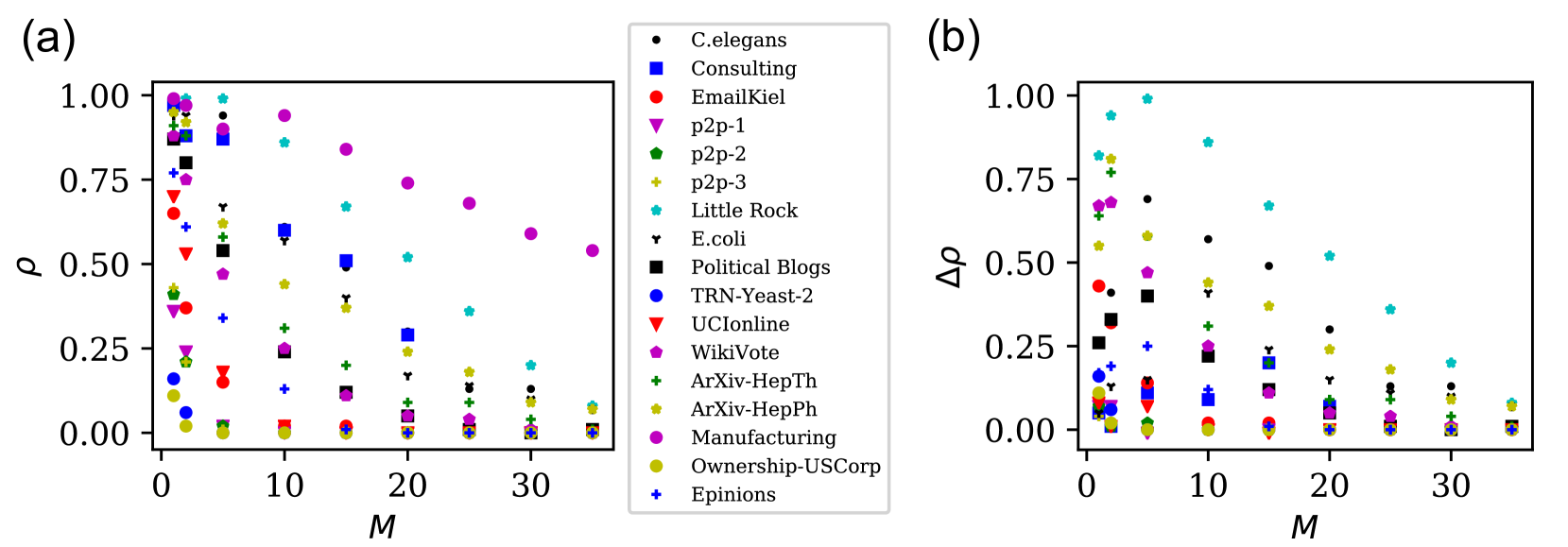
Figure 11: The sensor node placement algorithm can increase the probability of invertibility $\rho$, if the input node set is given (scenario SC 2). (a) The input node set was again uniformly sampled. All other nodes were considered as potential maximum output node set $Z_{0}$. In case of invertibility, the sensor node placement algorithm can reduce $Z_{0}$ to a minimum sensor node set $Z^{*}$ with $P^{*}=M$ outputs. (b) The difference $\Delta\rho$ between the probability of invertibility $\rho$ in (a) and the uniform random selection scheme used in Fig. 9(a) to highlight the improvement.

For the results in Fig. 11(a), we sampled $M$ input nodes $S$ uniformly from all nodes and then selected $Z_{0}$ as the remaining $N-M$ nodes (scenario SC 1 with the largest possible $Z_{0}$). We repeated this over 100 randomly sampled input sets $S$ and estimated the fraction $\rho$ of invertible systems $(S,g,Z_{0})$. Thus, $\rho$ provides an estimate for the probability to obtain a structurally invertible system (for a given graph $g$) under scenario SC 2, where the $M$ input nodes $S$ are given and cannot be chosen, but all the other nodes can in principle be measured. This is then identical to the fraction of systems, where the sensor node algorithm can reduce this initial sensor node set $Z_{0}$ to a minimum set $Z^{*}$ with $P^{*}=M$ outputs. By comparing Fig. 11(a) with Fig. 9(a) we can observe, that this strategy improves (in some cases drastically) the chances to find an invertible system. For better visibility see also Fig. 11(b), where we have plotted the difference $\Delta\rho$ between optimal sensor node placement in Fig. 11(a) and uniform output sampling Fig. 9(a).

V.3 Input node selection

So far we have assumed the input node set $S$ as given. To mimick this frequent situation that the input nodes can not deliberately be selected, we performed uniform random sampling of the input nodes. However, there might be situations where we can influence the selection of inputs (scenario SC 3). For the design of communication networks, the ability to uniquely distinguish different input signals is clearly a requirement and input node sets are often deliberately chosen Larsson (2014). Another example is given by the modular approach to model building, where one aims to describe a subsystem (or module) by a system of ODEs Raue et al. (2013); Almog and Korngreen (2016). This module will by definition receive inputs from the environment (see Fig. 1), which might not be directly measurable. Then, invertibility to infer these inputs from outputs is clearly an important requirement, which might influence decisions about the right state variables to include in the subsystem.

Based on the results of Fig. 8 we hypothesised that hubs with a high node degree are good candidates for inputs promoting invertibility. To test this hypothesis, we used again the networks listed in Table 1. For each network $g$, we selected the $M$ nodes with highest out-degree as input node set $S$. As before, we used the remaining $N-M$ nodes as maximum sensor node set $Z_{0}$. If $(S,g,Z_{0})$ is invertible, the sensor node selection algorithm can always reduce this to $(S,g,Z^{*})$ with a minimum node set $Z^{*}$ having only $P^{*}=M$ outputs. Starting from $M=1$ we increased the number of input nodes for each network one by one as long as the corresponding system $(S,g,Z_{0})$ was invertible. The maximum number $M_{\text{max}}$ of inputs for each network is shown in Fig. 12, together with the probability of invertibility for the other scenarios using the uniform random scheme (data from Fig. 9(a)) and the sensor node placement algorithm (data from Fig. 11(a)). Please note, that for this hub input selection strategy all systems with $M<M_{\text{max}}$ inputs are invertible. Clearly, the hub input selection strategy provides a way to increase the number of input signals which can still reconstructed in these networks.

Figure 12: A heatmap comparing the probability of invertibility $\rho$ for the networks in Table 1 with three different node selection schemes as a function of the number of inputs. Scenario SC 1, where neither inputs nor outputs can be selected, was simulated by uniform random sampling of input and output nodes (same data as in Fig. 9(a)). In scenario SC 2 we are able to select the output nodes and the results for the optimal sensor node placement from Fig. 11(a) are included for comparison. Under scenario scenario SC 3, we can select both, input and output nodes. We used hub input selection (selection of nodes with highest out-degree) in combination with optimal sensor node placement and found that $\rho$ is either one or zero. The numbers on the right indicate the maximum number $M_{\text{max}}$ of inputs which still provide an invertible system.

VI Summary and open questions

VI.1 Summary and significance of the results

Reconstructing unknown inputs from outputs of open systems is useful in many settings. For modellers, the inputs provide important information about model errors and cues for model improvement or extension Mook and Junkins (1988); Engelhardt et al. (2016, 2017). In biomedical systems, the unknown inputs can represent unmodelled environmental or physiological inputs, which might be interesting for the design of devices or measurement strategies. In electrical or secure networks, the unknown inputs could be attack signals, which need to be reconstructed and then mitigated. Unknown inputs can also be useful for improved state estimation Engelhardt et al. (2016, 2017); Chakrabarty et al. (2017) and data assimilation Abarbanel (2013); S. Reich and C. Cotter (2015). Thus, from the viewpoint of modellers and engineers, invertibility is a desirable property for open systems. In this work, we have focused on structural invertibility, which has the two advantages of (i) only requiring topological network information and (ii) being testable even for large networks using the structural controllability algorithm.

Although invertibility is desirable from an applied and analytic perspective, our results for an uniform random input selection scheme indicate that invertibility cannot be taken for granted, especially not in networks with low average degree, many inputs and with a scale free degree distribution. Thus, under the scenario SC 1, were neither inputs nor outputs can deliberately be chosen, many real networks have a disposition to mask differences between different input signals. It is well known that for example some dynamic biological systems respond often identically or similarly to a variety of different stimuli. Thus, living dynamic systems often distinguish different patterns rather than small differences in the inputs. In addition, real systems need to have a certain robustness against small perturbations and noise. Thus, invertibility is possibly not always a desirable property for the specific tasks to be performed by the network. Further research is needed to investigate tradeoffs between invertibility and other network traits, like e.g. controllability or robustness. Nevertheless, non-invertibility poses a challenge for experimentalists and modellers to reconstruct structural model errors and inputs from the environment.

We approached this problem by deriving an efficient sensor node placement algorithm, which extracts a minimum set of measurement nodes required for invertibility of a given network with a given input set (scenario SC 2). In this scenario, the sensor node placement algorithm facilitates optimal experimental design for the reconstruction of inputs from outputs. As such, it can be used in conjunction with input reconstruction algorithms Kühl et al. (2011); Raue et al. (2012); Fonod et al. (2014); Engelhardt et al. (2016, 2017) and input observers Chakrabarty et al. (2017); Tsiantis et al. (2018). Structural invertibility provides a necessary condition for these algorithms to work.

In a third scenario SC 3 we assumed that both inputs and outputs can be selected. We found that selecting nodes with a high out-degree as input nodes, in combination with optimal output selection using the sensor node placement algorithm, drastically increases the number of inputs which can still be reconstructed from output measurements. Intuitively, these input hubs distribute the input signal widely over the network, therefore increasing the likelihood for finding node disjoint paths linking these inputs to the outputs. Although scenario SC 3, where input nodes can deliberately be selected, might not always be realistic, it can be useful for the design of dynamic mathematical models or for the design of synthetic systems. For example, a key goal of Synthetic Biology is to engineer new biological systems for desired functionalities. In general, these systems are embedded in larger systems and will receive inputs from their environment, which should be inferable from measurements. In this case, optimal input selection in conjunction with optimal sensor node placement can provide important benefits. Another example is modular modelling, were an interesting subsystem embedded in a larger system is modelled in detail Raue et al. (2013); Almog and Korngreen (2016). To detect both potential model error or genuine inputs from the environment to the model, invertibility is essential. To achieve invertibility, it might be useful to include additional states which otherwise would not be deemed to be essential to understand the modular subsystem.

VI.2 Limitations and open questions

Purely structural approaches to controllability and observability have been criticised to sometimes provide suboptimal conclusions for real systems. Depending on the quantitative properties of the interactions between the state nodes, a system might be practically uncontrollable or unobservable, even if the structural criteria are fulfilled Krener and Kayo (2009); Cornelius et al. (2011); Sun and Motter (2013); Cornelius et al. (2013); Yan et al. (2015); Lo Iudice et al. (2015); Summers et al. (2016); Klickstein et al. (2017); Aguirre et al. (2018); Haber et al. (2018). Non-binary indices quantifying the degree of controllability and observability have been devised. These indices require at least the algebraic structure of the coupling functions between the state nodes Aguirre et al. (2018) or even the full functional form and the parameters of the network Cornelius et al. (2013).

A similar caveat applies to structural invertibility, which is only a condition for the existence of the inverse input-output map. As in any inverse problem  G. Nakamura and R. Potthast (2015), this might not be sufficient to actually implement this inverse map for reconstructing unknown inputs (including model errors) from outputs. Some unknown input signals might be hard to detect by noisy sensors with limited sensitivity. As discussed in Subsec. III.7, these issues are related to the mathematical fact that the inverse of the compact input-output map is not continuous. Devising an index or condition number for the degree of invertibility (or continuity of the inverse) is therefore an important question for future research. Such an invertibility index might be used to rank sensor nodes, which could readily be utilised in a straightforward modification of our sensor node placement algorithm (Sec. V). The desired invertibility index might also be useful for improving or designing unknown input reconstruction algorithms  Kühl et al. (2011); Raue et al. (2012); Fonod et al. (2014); Engelhardt et al. (2016, 2017); Chakrabarty et al. (2017); Tsiantis et al. (2018), which adapt their regularisation automatically to the degree of discontinuity of the inverse input-output map.

A further potential objection against structural invertibility is that the influence graph has to be completely known. Indeed, if the aim is to assess invertibility of the true but unknown systems structure, we might obtain erroneous results if we use an incorrect influence graph with missing or spurious edges. However, the aim of systems inversion is to detect unknown inputs including systematic model errors. Missing or spurious interactions in the incorrect model graph are therefore causes of unknown inputs. To reconstruct the model errors, it is important that our potentially incorrect or incomplete model is invertible.

Currently, our invertibility results are limited to deterministic systems described by ODEs. However, the definition of invertibility doesn’t exclude stochastic unknown unput functions. Nonlinear extensions of the Kalman-Filter Kühl et al. (2011); Raue et al. (2012); Fonod et al. (2014) or fully probabilistic approaches  Engelhardt et al. (2017) to reconstruct the moments or even the full probability distribution of the unknown input will only work for invertible systems. Their actual utility to simultaneously overcome the discontinuity of the inverse input-output map and to estimate probabilistic features of unknown inputs should systematically be explored.

Invertibility of systems with intrinsic process noise, which are often described by stochastic differential equations (SDEs), is a largely unexplored field. First, a modified probabilistic definition of invertibility is required for systems governed by SDEs. Second, the role of the different sources of noise for the invertibility needs to be investigated. Recent results for stochastic synchronisation Russo and Shorten (2018); Burbano-L. et al. (2019) indicate, that noise can have both, detrimental and beneficial effects. It would be exciting to investigate, whether similar effects are possible for unknown input reconstruction.

To conclude, invertibility (or the lack of it) has important implications for modelling frameworks and strategies to deal with incomplete and uncertain systems. Our analysis and algorithm for optimal experimental design are only a first step towards more sophisticated methods specifically tailored to handle systematic model errors and open systems. We belive that these approaches will increase our ability to better understand and manipulate complex systems, even if our knowledge will not be complete.

*

Appendix A Derivation of the Algebraic Criterion

For the sake of completeness let us explicitly write down the general mathematical setting for the linear case in our notation and deduce the algebraic criterion. In the general linear case, the initial state is given by a vector ${\mbox{$x$}}_{0}\in\mathbb{R}^{N}$, the dynamic of the system is given by $A\in\mathbb{R}^{N\times N}$, and $C\in\mathbb{R}^{P\times N}$ maps the system state to the output. There might be a known input ${\mbox{$u$}}:[0,T]\to\mathbb{R}^{M^{\prime}}$ distributed by $B\in\mathbb{R}^{N\times M^{\prime}}$ over the state variables. Finally $D{\mbox{$w$}}$ models the structural model errors, so that we get the linear dynamic system,

$$\dot{{\mbox{$x$}}}(t) = A{\mbox{$x$}}(t)+B{\mbox{$u$}}(t)+D{\mbox{$w$}}(t)$$ (34a)

$${\mbox{$x$}}(0) = {\mbox{$x$}}_{0}$$ (34b)

$${\mbox{$y$}}(t) = C{\mbox{$x$}}(t)\,.$$ (34c)

Let $\Phi:{\mbox{$w$}}\mapsto{\mbox{$y$}}$ denote the solution operator, that maps the input $w$ to the output $y$ according to the dynamic system (34). For the dynamic system (34) we introduce the homogeneous system

$$\dot{{\mbox{$x$}}}(t) = A{\mbox{$x$}}(t)+D{\mbox{$w$}}(t)$$ (35a)

$${\mbox{$x$}}(0) = 0$$ (35b)

$${\mbox{$y$}}(t) = C{\mbox{$x$}}(t)$$ (35c)

with the solution operator $\Phi^{\text{hom}}:{\mbox{$w$}}\mapsto{\mbox{$y$}}$. Recall that a system is called invertible if for given data

$${\mbox{$y$}}^{\text{obs}}:[0,T]\to\mathbb{R}^{P}$$ (36)

any solution of

$$\Phi({\mbox{$w$}})(t)={\mbox{$y$}}^{\text{obs}}(t)\quad\forall\,t\in[0,T]$$ (37)

is unique. We will make use of the Volterra-operator

$$V({\mbox{$w$}})(t):=\int_{0}^{t}{\mbox{$w$}}(s)\,\text{d}s\,.$$ (38)

The Volterra-operator has the property

$$V^{n}({\mbox{$w$}})(t)=\int\limits_{0}^{t}\frac{(t-s)^{n-1}}{(n-1)!}{\mbox{$w$}}(s)\,\text{d}s$$ (39)

and hence

$$\sum_{n=0}^{\infty}CA^{n}DV^{n+1}({\mbox{$w$}})(t)$$ (40)

$$\quad=\int\limits_{0}^{t}C\exp((t-s)A)D{\mbox{$w$}}(s)\,\text{d}s\,,$$

where the integration is understood component-wise.

Lemma 1.

Let $\Phi$ and $\Phi^{\text{hom}}$ be the solution operators of a dynamic system as defined above. Then

1. $\Phi^{\text{hom}}$ is linear, continuous, and compact,

2. $\Phi(w+v)=\Phi(w)$ if and only if $\Phi^{\text{hom}}(v)=0$.

Proof.

1. The homogeneous solution operator takes the form

   $$\Phi^{\text{hom}}=\sum_{n=0}^{\infty}(CA^{n}D)V^{n+1}\quad.$$ (41)

   To see this, let

   $${\mbox{$x$}}(t)=\sum_{n=0}^{\infty}A^{n}DV^{n+1}({\mbox{$w$}})(t)$$ (42)

   then

   $$\frac{\text{d}}{\text{d}t}{\mbox{$x$}}(t) =D{\mbox{$w$}}(t)+A\sum_{n=1}^{\infty}A^{n-1}DV^{n}({\mbox{$w$}})(t)$$ (43)

   $$=D{\mbox{$w$}}(t)+A{\mbox{$x$}}(t)$$ (44)

   which shows that $x$ solves the dynamic equations as well as ${\mbox{$x$}}(0)=0$. Multiplication with $C$ yields the solution of the homogeneous system

   $${\mbox{$y$}}(t)=\Phi^{\text{hom}}({\mbox{$w$}})(t)\quad.$$ (45)

   Since $V^{n}$ is linear, so is $\Phi^{\text{hom}}$. As we make the restriction $w_{i}\in L^{2}([0,T])$ we get that $\Phi^{\text{hom}}$ is Hilbert-Schmidt thus continuous and compact.

2. The inhomogeneous part of $\Phi$ is given by

   $$\begin{aligned} \phi(t):=&\sum_{n=0}^{\infty}CA^{n}DV^{n+1}({\mbox{$u$}})(t)\\ &+\exp(At){\mbox{$x$}}_{0}\end{aligned}\,,$$ (46)

   such that the full solution can be written as

   $$\Phi({\mbox{$w$}})(t)=\phi(t)+\Phi^{\text{hom}}({\mbox{$w$}})(t)$$ (47)

   which shows that

   $$\Phi({\mbox{$w$}}+{\mbox{$v$}})=\Phi({\mbox{$w$}})+\Phi^{\text{hom}}({\mbox{$v$}})$$ (48)

   hence if and only if $\Phi^{\text{hom}}({\mbox{$v$}})=0$ then $v$ leaves the solution of the inhomogeneous system invariant.

∎

As a result of the above lemma, we can set ${\mbox{$x$}}_{0}$ as well as $u$ to zero. Furthermore this shows that $\Phi$ given in Sec. III is indeed the relevant solution operator that has to be one-to-one. We now follow the proof of Sain and Massey M. Sain  and J. Massey (1969). After Laplace-transformation the dynamic equation becomes

$$s\mathcal{L}[{\mbox{$x$}}](s)=A\mathcal{L}[{\mbox{$x$}}](s)+D\mathcal{L}[{\mbox{$w$}}](s)$$ (49)

with a complex variable $s\in\mathbb{C}$. Using the transfer function

$$T(s):=C(\mathbb{I}s-A)^{-1}D\,,$$ (50)

where $\mathbb{I}$ is the identity in $\mathbb{R}^{N}$, we get

$$T(s)\mathcal{L}[{\mbox{$w$}}](s)=\mathcal{L}[y](s)$$ (51)

thus $T$ is the Laplace-transform of the solution operator $\Phi$, and since $\mathcal{L}[{\mbox{$w$}}]$ is the zero function if and only if $w$ is the zero-function (almost everywhere), we know that $\Phi$ is one-to-one if and only if $T$ has $\text{rank}\,T(s)=M$ for $s\in\mathbb{C}$ (almost everywhere), i.e. if from $\mathcal{L}[{\mbox{$y$}}]=0$ it follows, that $\mathcal{L}[{\mbox{$w$}}]=0$. We make the assumption, that $w$ is smooth, which is equivalent to the assumption, that it can be written as a Laurent-series (comprising only the principal part)

$$\mathcal{L}[{\mbox{$w$}}](s)=\frac{1}{s}\sum\limits_{k=0}^{\infty}\frac{1}{s^{k}}\xi_{k}$$ (52)

in Laplace-space, where $(\xi_{k})_{k}$ is a sequence of $\mathbb{R}^{M}$ vectors. Using the Neumann-series yields

$$C(\mathbb{I}s-A)^{-1}D=\frac{1}{s}\sum\limits_{l=0}^{\infty}C\frac{A^{l}}{s^{l}}D\,.$$ (53)

If $\mathcal{L}[{\mbox{$y$}}]=0$, then

$$\frac{1}{s^{2}}\sum\limits_{k,l=0}^{\infty}\frac{1}{s^{l+k}}CA^{l}D\xi_{k}=0$$ (54)

and since $\{1,s^{-1},s^{-2},\ldots\}$ are linearly independent in function space, by equating coefficients for each $n\in\mathbb{N}_{0}$ we find

$$\sum\limits_{k=0}^{n}CA^{k}D\xi_{n-k}=0\,.$$ (55)

It is now convenient to define

$$R_{n}:=\begin{bmatrix}CD&CAD&\ldots&CA^{n}D\end{bmatrix}$$ (56)

as known from the Kalman controllability matrix, as well as

$$\Xi_{n}:=\begin{bmatrix}\xi_{n}\\ \vdots\\ \xi_{0}\end{bmatrix}$$ (57)

to finally get

$$R_{n}\Xi_{n}=0\,\forall n\in\mathbb{N}_{0}\,.$$ (58)

Thus, the dynamic system is invertible if and only if we find a sequence $(\xi_{k})_{k}$ such that (58) holds. If we combine $R_{0},R_{1},\ldots,R_{l}$ to one matrix

$$Q_{l}:=\begin{bmatrix}CD&CAD&\dots&CA^{l}D\\ 0&CD&\dots&CA^{l-1}D\\ \vdots&&\ddots&\vdots\\ 0&\dots&&CD\end{bmatrix}\quad.$$ (59)

we find, that (58) is equivalent to

$$\text{rank}\,Q_{N-1}-\text{rank}\,Q_{N-2}=M\,,$$ (60)

the criterion stated by Sain and Massey. From (58) we directly see, that $\Xi_{l}\in\ker R_{l}$ and $\Xi_{l+1}\in\ker R_{l+1}$. Also $\Xi_{l+1}=[\xi_{l+1},\Xi_{l}]^{T}$, thus

$$\Xi_{l+1}\in\ker R_{l+1}\cap\left(\mathbb{R}^{M}\times\ker R_{l}\right)\,.$$ (61)

If we now exclude the trivial solution $\xi_{l}=0$ for all $l$, this motivates

$$K_{0}:=\ker R_{0}\backslash\{0\}$$ (62)

and

$$K_{l}:=\ker R_{l+1}\cap\left(\mathbb{R}^{M}\times K_{l}\right)\,.$$ (63)

As we iterate though $K_{0},K_{1},\ldots$, as long as $K_{l}\neq\emptyset$ there is a non-trivial solution of

$$R_{k}\Xi_{k}=0\text{ for }k\leq l\,.$$ (64)

Hence, if and only if we find a $l\in\mathbb{N}_{0}$, such that $R_{l}=\emptyset$, then the dynamic system is invertible. From (60) one can see, that is suffices to check only $l\leq N-1$. In addition to that we find the following theorem.

Theorem 1.

The solution space of

$$\Phi({\mbox{$w$}})={\mbox{$y$}}^{\text{obs}}$$ (65)

is either zero- or infinite-dimensional.

Proof.

From the considerations above it is clear, that we have to show that the solution space of (58) is either zero- or infinite-dimensional, i.e. if there is a non-trivial sequence $(\xi_{k})_{k}$, then there is an infinite-dimensional vector space of such sequences.

First, assume $(\xi_{k})_{k}$ is a sequence, that solves (58) and $\xi_{0}=0$. We define another sequence $(\chi_{k})_{k}$ by $\chi_{k}:=\xi_{k+1}$, i.e. $(\chi_{k})_{k}$ is the left shift of $(\xi_{k})_{k}$. Let $X_{l}$ the vector $[\chi_{l},\ldots,\chi_{0}]^{T}$ analogous to $\Xi_{l}$. Then

$$0=R_{l}\Xi_{l}=R_{l-1}X_{l-1}$$ (66)

for all $l$. Hence $(\chi_{k})_{k}$ is also a solution. This shows, that if $(\xi_{k})_{k}$ solves (58), then we can without loss of generality assume $\xi_{0}\neq 0$.

Now let $(\xi_{k})_{k}$ a solution and define $\chi_{0}:=0$ and $\chi_{k}=\xi_{k-1}$, i.e. $(\chi_{k})_{k}$ is the right shift of $(\xi_{k})_{k}$. Then

$$R_{0}X_{0}=0$$ (67)

is clear, and for $l\geq 1$

$$R_{l}X_{l}=R_{l-1}\Xi_{l-1}=0$$ (68)

hence the sequence $(\chi_{k})_{k}$ solves (58). Let henceforth $\mathfrak{S}_{\rightarrow}$ denote the right shift.

Since matrix multiplication is a linear operation it is clear, that if $(\xi_{k})_{k}$ and $(\chi_{k})_{k}$ solve (58), so does $(\xi_{k}+\chi_{k})_{k}$ as well as $(a\xi_{k})_{k}$ for an arbitrary real number $a$. Therefore the space of sequences that solve (58) is a real vector space, denoted $\mathcal{K}$. Let $(\xi_{k})_{k}\in\mathcal{K}$ with $\xi_{0}\neq 0$. Then $\mathfrak{S}_{\rightarrow}^{q}(\xi_{k})_{k}\in\mathcal{K}$ and

$$\{(\xi_{k})_{k},\mathfrak{S}_{\rightarrow}(\xi_{k})_{k},\mathfrak{S}_{\rightarrow}^{2}(\xi_{k})_{k},\ldots\}$$ (69)

is a set of infinitely many linearly independent vectors in $\mathcal{K}$, hence

$$\dim\mathcal{K}=\infty\,.$$ (70)

∎

References

- Raue et al. (2013) A. Raue, M. Schilling, J. Bachmann, A. Matteson, M. Schelke, D. Kaschek, S. Hug, C. Kreutz, B. D. Harms, F. J. Theis, U. Klingmüller, and J. Timmer, Lessons Learned from Quantitative Dynamical Modeling in Systems Biology, PLOS ONE 8, 1 (2013).
- Almog and Korngreen (2016) M. Almogand A. Korngreen, Is realistic neuronal modeling realistic?, Journal of Neurophysiology 116, 2180 (2016).
- Papin et al. (2017) J. A. Papin, J. J. Saucerman, S. M. Peirce, K. A. Janes, P. L. Chandran, M. J. Lazzara, R. M. Ford, and D. A. Lauffenburger, An engineering design approach to systems biology, Integrative Biology 9, 574 (2017).
- Tsigkinopoulou et al. (2017) A. Tsigkinopoulou, S. M. Baker, and R. Breitling, Respectful Modeling: Addressing Uncertainty in Dynamic System Models for Molecular Biology, Trends in Biotechnology 35, 518 (2017).
- Rossi and Ahmed (2015) R. A. Rossi and N. K. Ahmed, The Network Data Repository with Interactive Graph Analytics and Visualization, in Proceedings of the Twenty-Ninth AAAI Conference on Artificial Intelligence, AAAI’15 (AAAI Press, 2015) pp. 4292–4293.
- (6) V. Batagelj and A. Mrvar, Pajek datasets, http://vlado.fmf.uni-lj.si/pub/networks/data/, access date 2018-12-16.
- Kunegis (2013) J. Kunegis, KONECT - The Koblenz Network Collection, in Proc. Int. Web Observatory Workshop (2013) pp. 1343–1350.
- (8) J. Leskovec and A. Krevl, SNAP Datasets: Stanford Large Network Dataset Collection, http://snap.stanford.edu/data, access date 2018-12-16.
- Kühl et al. (2011) P. Kühl, M. Diehl, T. Kraus, J. P. Schlöder, and H. G. Bock, A real-time algorithm for moving horizon state and parameter estimation, Computers & Chemical Engineering 35, 71 (2011).
- Raue et al. (2012) A. Raue, C. Kreutz, M. Schelker, and J. Timmer, Comprehensive estimation of input signals and dynamics in biochemical reaction networks, Bioinformatics 28, i529 (2012).
- Fonod et al. (2014) R. Fonod, D. Henry, C. Charbonnel, and E. Bornschlegl, A Class of Nonlinear Unknown Input Observer for Fault Diagnosis: Application to Fault Tolerant Control of an Autonomous Spacecraft, in 10th UKACC International Conference on Control (IEEE, Loughborough, United Kingdom, 2014) pp. 19–24.
- Engelhardt et al. (2016) B. Engelhardt, H. Fröhlich, and M. Kschischo, Learning (from) the errors of a systems biology model, Scientific Reports 6, 20772 (2016).
- Engelhardt et al. (2017) B. Engelhardt, M. Kschischo, and H. Fröhlich, A Bayesian approach to estimating hidden variables as well as missing and wrong molecular interactions in ordinary differential equation-based mathematical models, Journal of The Royal Society Interface 14, 20170332 (2017).
- Chakrabarty et al. (2017) A. Chakrabarty, M. J. Corless, G. T. Buzzard, S. H. Zak, and A. E. Rundell, State and Unknown Input Observers for Nonlinear Systems With Bounded Exogenous Inputs, IEEE Transactions on Automatic Control 62, 5497 (2017).
- Tsiantis et al. (2018) N. Tsiantis, E. Balsa-Canto, and J. R. Banga, Optimality and identification of dynamic models in systems biology: an inverse optimal control framework, Bioinformatics 34, 2433 (2018).
- Ebrahim et al. (2015) A. Ebrahim, J. A. Lerman, J. Lu, P. Miller, S. Federowicz, Z. A. King, A. Dräger, B. O. Palsson, and N. E. Lewis, BiGG Models: A platform for integrating, standardizing and sharing genome-scale models, Nucleic Acids Research 44, D515 (2015).
- Lin (1974) C.-T. Lin, Structural controllability, IEEE Transactions on Automatic Control 19, 201 (1974).
- Liu et al. (2011) Y.-Y. Liu, J.-J. Slotine, and A.-L. Barabási, Controllability of complex networks, Nature 473, 167 (2011).
- Liu et al. (2013) Y.-Y. Liu, J.-J. Slotine, and A.-L. Barabási, Observability of complex systems, in Proceedings of the National Academy of Sciences, Vol. 110 (2013) pp. 2460–2465.
- Gao et al. (2014) J. Gao, Y.-Y. Liu, R. M. D’Souza, and A.-L. Barabási, Target control of complex networks, Nature Communications 5, 5415 (2014).
- Motter (2015) A. E. Motter, Networkcontrology, Chaos: An Interdisciplinary Journal of Nonlinear Science 25, 097621 (2015).
- Liu and Barabási (2016) Y.-Y. Liu and A.-L. Barabási, Control principles of complex systems, Rev. Mod. Phys. 88, 035006 (2016).
- Sharma et al. (2017) A. Sharma, C. Cinti, and E. Capobianco, Multitype Network-Guided Target Controllability in Phenotypically Characterized Osteosarcoma: Role of Tumor Microenvironment, Frontiers in Immunology 8, 918 (2017).
- Krener and Kayo (2009) A. J. Krenerand I. Kayo, Measures of unobservability, IEEE Conf. Decis. Control (2009).
- Lo Iudice et al. (2015) F. Lo Iudice, F. Garofalo, and F. Sorrentino, Structural permeability of complex networks to control signals, Nature Communications 6, 8349 (2015).
- Klickstein et al. (2017) I. Klickstein, A. Shirin, and F. Sorrentino, Energy scaling of targeted optimal control of complex networks, Nature Communications 8, 15145 (2017).
- Cornelius et al. (2011) S. P. Cornelius, W. L. Kath, and A. E. Motter, Controlling Complex Networks with Compensatory Perturbations, arXiv:1105.3726 (2011).
- Sun and Motter (2013) J. Sun and A. E. Motter, Controllability Transition and Nonlocality in Network Control, Phys. Rev. Lett. 110, 208701 (2013).
- Cornelius et al. (2013) S. P. Cornelius, W. L. Kath, and A. E. Motter, Realistic control of network dynamics, Nature Communications 4, 1942 (2013).
- Yan et al. (2015) G. Yan, G. Tsekenis, B. Barzel, J.-J. Slotine, Y.-Y. Liu, and A.-L. Barabási, Spectrum of controlling and observing complex networks, Nature Physics 11, 779 (2015).
- Summers et al. (2016) T. H. Summers, F. L. Cortesi, and J. Lygeros, On Submodularity and Controllability in Complex Dynamical Networks, IEEE Transactions on Control of Network Systems 3, 91 (2016).
- Aguirre et al. (2018) L. A. Aguirre, L. L. Leonardo, and C. Letellier, Structural, dynamical and symbolic observability: From dynamical systems to networks, PLoS ONE 13, 1 (2018).
- Haber et al. (2018) A. Haber, F. Molnar, and A. E. Motter, State Observation and Sensor Selection for Nonlinear Networks, IEEE Transactions on Control of Network Systems 5, 694 (2018).
- Mook and Junkins (1988) D. J. Mook and J. L. Junkins, Minimum model error estimation for poorly modeled dynamic systems, Journal of Guidance, Control, and Dynamics 11, 256 (1988).
- R. W. Brockett and M. D. Mesarović (1965) R. W. Brockett and M. D. Mesarović, The reproducibility of multivariable systems, Journal of Mathematical Analysis and Applications 11, 548 (1965).
- Silverman (1969) L. Silverman, Inversion of multivariable linear systems, IEEE Transactions on Automatic Control 14, 270 (1969).
- M. Sain and J. Massey (1969) M. Sain and J. Massey, Invertibility of linear time-invariant dynamical systems, IEEE Transactions on Automatic Control 14, 141 (1969).
- Hirschorn (1979) R. M. Hirschorn, Invertibility of Nonlinear Control Systems, SIAM Journal on Control and Optimization 17, 289 (1979).
- Nijmeijer (1982) H. Nijmeijer, Invertibility of affine nonlinear control systems: A geometric approach, Systems & Control Letters 2, 163 (1982).
- Nijmeijer (1986) H. Nijmeijer, Right-invertibility for a class of nonlinear control systems: A geometric approach, Systems & Control Letters 7, 125 (1986).
- Fliess (1986) M. Fliess, A note on the invertibility of nonlinear input-output differential systems, Systems & Control Letters 8, 147 (1986).
- Wey (1998) T. Wey, Rank and Regular Invertibility of Nonlinear Systems: A Graph Theoretic Approach, IFAC Proceedings Volumes 31, 257 (1998).
- Dion et al. (2003) J.-M. Dion, C. Commault, and J. van der Woude, Generic properties and control of linear structured systems: a survey, Automatica 39, 1125 (2003).
- Boukhobza et al. (2007) T. Boukhobza, F. Hamelin, and S. Martinez-Martinez, State and input observability for structured linear systems: A graph-theoretic approach, Automatica 43, 1204 (2007).
- Moreno et al. (2014) J. A. Moreno, E. Rocha-Cózatl, and A. V. Wouwer, A dynamical interpretation of strong observability and detectability concepts for nonlinear systems with unknown inputs: application to biochemical processes, Bioprocess and Biosystems Engineering 37, 37 (2014).
- Milo et al. (2002) R. Milo, S. Shen-Orr, S. Itzkovitz, N. Kashtan, D. Chklovskii, and U. Alon, Network Motifs: Simple Building Blocks of Complex Networks, Science 298, 824 (2002).
- Martinelli (2019) A. Martinelli, Nonlinear Unknown Input Observability: The General Analytic Solution , IEEE Trans. Automat. Contr. 64, 222 (2019), arXiv: 1704.03252.
- Menger (1927) K. Menger, Zur allgemeinen Kurventheorie, Fund. Math. 10, 96 (1927).
- B. Korte and J. Vygen (2018) B. Korte and J. Vygen, Combinatorial optimization: theory and algorithms, sixth edition ed., Algorithms and combinatorics No. 21 (Springer, Berlin, Germany, 2018).
- A. Goldberg (1988) R. T. A. Goldberg, A new approach to the maximum flow problem, Journal of the ACM. 35, 921 (1988).
- Engl et al. (2000) H. Engl, M. Hanke, and A. Neubauer, Regularization of Inverse Problems (Springer Netherlands, Kluwer Academic Publishers, Dordrecht, 2000).
- G. Nakamura and R. Potthast (2015) G. Nakamura and R. Potthast, An introduction to the theory and methods of inverse problems and data assimilation, IOP Expanding Physics (Institute of Physics Publishing, 2015).
- Abarbanel (2013) H. D. I. Abarbanel, Predicting the future: completing models of observed complex systems, Understanding complex systems (Springer, New York, NY, 2013).
- P. Erdős and A. Rényi (1960) P. Erdős and A. Rényi, On the evolution of random graphs, Publ. Math. Inst. Hung. Acad. Sci. 5, 17 (1960).
- A.-L. Barabási and R. Albert (1999) A.-L. Barabási and R. Albert, Emergence of scaling in random networks, Science 286, 509 (1999).
- Goh et al. (2001) K.-I. Goh, B. Kahng, and D. Kim, Universal Behavior of Load Distribution in Scale-Free Networks, Phys. Rev. Lett. 87, 278701 (2001).
- R. Cohen and S. Havlin (2003) R. Cohen and S. Havlin, Scale-Free Networks Are Ultrasmall, Physical Review Letters 90, 058701 (2003).
- Schellenberger et al. (2010) J. Schellenberger, J. O. Park, T. M. Conrad, and B. Ø. Palsson, BiGG: a Biochemical Genetic and Genomic knowledgebase of large scale metabolic reconstructions, BMC Bioinformatics 11, 213 (2010).
- S. Maslov and K. Sneppen (2002) S. Maslov and K. Sneppen, Specificity and Stability in Topology of Protein Networks, Science 296, 910 (2002).
- (60) U. Alon, Collection of complex networks, http://www.weizmann.ac.il/mcb/UriAlon/download/collection-complex-networks, access date 2018-12-16.
- Norlen et al. (2002) K. Norlen, G. Lucas, M. Gebbie, and J. Chuang, EVA: Extraction, Visualization and Analysis of the Telecommunications and Media Ownership Network, in Proceedings of International Telecommunications Society 14th Biennial Conference (ITS2002), Seoul Korea (2002) pp. 27–129.
- Leskovec et al. (2009) J. Leskovec, K. J. Lang, A. Dasgupta, and M. W. Mahoney, Community Structure in Large Networks: Natural Cluster Sizes and the Absence of Large Well-Defined Clusters, Internet Mathematics 6, 29 (2009).
- Richardson et al. (2003) M. Richardson, R. Agrawal, and P. Domingos, Trust Management for the Semantic Web, in The Semantic Web - ISWC 2003, edited by D. Fensel, K. Sycara, and J. Mylopoulos (Springer Berlin Heidelberg, Berlin, Heidelberg, 2003) pp. 351–368.
- Martinez (1991) N. D. Martinez, Artifacts or Attributes? Effects of Resolution on the Little Rock Lake Food Web, Ecological Monographs 61, 367 (1991).
- (65) M. S. Ma’ayan Laboratory Department of Pharmacologyand S. Therapeutics, http://research.mssm.edu/maayan/datasets/qualitative_networks.shtml, access date 2018-12-16.
- (66) BiGG Models, http://bigg.ucsd.edu, access date 2018-12-16.
- D. J. Watts and S. H. Strogatz (1998) D. J. Watts and S. H. Strogatz, Collective dynamics of ‘small-world’ networks, Nature 393, 440 (1998).
- Leskovec et al. (2005) J. Leskovec, J. Kleinberg, and C. Faloutsos, Graphs over time: densification laws, shrinking diameters and possible explanations, in Proceeding of the eleventh ACM SIGKDD international conference on Knowledge discovery in data mining - KDD ’05 (ACM Press, 2005) p. 177.
- L. A. Adamic and N. Glance (2005) L. A. Adamic and N. Glance, The political blogosphere and the 2004 U.S. election: divided they blog, in Proceedings of the 3rd international workshop on Link discovery - LinkKDD ’05 (ACM Press, 2005) pp. 36–43.
- Datasets (a) Datasets, http://moreno.ss.uci.edu/data.html#blogs, access date 2018-12-16 (a).
- Leskovec et al. (2007) J. Leskovec, J. Kleinberg, and C. Faloutsos, Graph evolution: Densification and shrinking diameters, ACM Transactions on Knowledge Discovery from Data 1, 2 (2007).
- T. Opsahl and P. Panzarasa (2009) T. Opsahl and P. Panzarasa, Clustering in weighted networks, Social Networks 31, 155 (2009).
- Datasets (b) Datasets, https://toreopsahl.com/datasets/, access date 2018-12-16 (b).
- Ebel et al. (2002) H. Ebel, L.-I. Mielsch, and S. Bornholdt, Scale-free topology of e-mail networks, Physical Review E 66, 10.1103/PhysRevE.66.035103 (2002).
- R. L. Cross and A. Parker (2004) R. L. Cross and A. Parker, The hidden power of social networks: understanding how work really gets done in organizations (Harvard Business School Press, Boston, Mass, 2004).
- Larsson (2014) C. Larsson, Design of modern communication networks: methods and applications, 1st ed. (Academic Press/Elsevier, Amsterdam, 2014) oCLC: 907438989.
- S. Reich and C. Cotter (2015) S. Reich and C. Cotter, Probabilistic forecasting and Bayesian data assimilation (Cambridge University Press, Cambridge, 2015).
- Russo and Shorten (2018) G. Russo and R. Shorten, On common noise-induced synchronization in complex networks with state-dependent noise diffusion processes, Physica D Nonlinear Phenomena 369, 47 (2018).
- Burbano-L. et al. (2019) D. A. Burbano-L., G. Russo, and M. D. Bernardo, Pinning Controllability of Complex Network Systems With Noise, IEEE Transactions on Control of Network Systems 6, 874 (2019).