Online Learning Algorithms for Quaternion ARMA Model

Abstract

In this paper, we address the problem of adaptive learning for autoregressive moving average (ARMA) model in the quaternion domain. By transforming the original learning problem into a full information optimization task without explicit noise terms, and then solving the optimization problem using the gradient descent and the Newton analogues, we obtain two online learning algorithms for the quaternion ARMA. Furthermore, regret bound analysis accounting for the specific properties of quaternion algebra is presented, which proves that the performance of the online algorithms asymptotically approaches that of the best quaternion ARMA model in hindsight.

1 Introduction

In recent years, quaternion algebra has attracted considerable attention in the signal processing community. As a natural representation of 3D and 4D signals, quaternion allows for a reduction in the number of parameters and operations involved, and can bring insights that would not be acquired by real- and complex-valued representations. Due to these elegant properties, quaternion adaptive signal processing algorithms have developed rapidly and have achieved satisfactory performance in a wide range of applications [1, 2, 3, 4, 5, 6, 7, 8].

Despite the existence of many quaternion algorithms, we notice that so far, there is no learning algorithm for the ARMA model in the quaternion domain. Due to its flexibility in the modeling of actual time series, the ARMA has been widely used in the real and complex domains for modeling 1D and 2D time series [9, 10, 11, 12, 13]. Thus, when it comes to 3D and 4D situations, a natural idea is to extend the ARMA model and its learning algorithms to the quaternion domain in order to take advantage of quaternion-valued representation.

To this end, in this paper, we propose two online learning algorithms for the quaternion ARMA (qARMA) model. The online learning is achieved by borrowing the idea of “improper learning” principle[14, 15] in the real domain, and transforming the learning problem of qARMA into a full information optimization task without explicit noise terms. We then solve the optimization problem by extending the online gradient descent method [16] and the online Newton method [17] to the quaternion domain. Furthermore, we present regret bound analysis of the proposed method to illustrate the validity of this transformation, which, to the best of our knowledge, is the first time that regret bound analysis for quaternion algorithms is performed. The theoretical results guarantee that the performance of the online algorithms asymptotically approaches that of the best quaternion ARMA model in hindsight.

2 Preliminaries

2.1 Notations

In this letter, for a quaternion vector $q=q_{a}+q_{b}i+q_{c}j+q_{d}k\in\mathbf{H}^{n}$, expressed by its real coordinate vectors $q_{a},q_{b},q_{c}$, and $q_{d}\in\mathbf{R}^{n}$, we use $q^{*}$ to denote its conjugate, $q^{i},q^{j},q^{k}$ to denote its involution [18], $q^{T}$ to denote its transpose, and $q^{H}$ to denote its Hermintian transpose. We use $\left\|q\right\|=\sqrt{q^{H}q}$ to denote its norm. We use underlined letter $\underline{q}=[q^{T},q^{iT},q^{jT},q^{kT}]^{T}\in\mathbf{H}^{4n}$ to denote its augmented quaternion vector [2], and $r_{q}=[q_{a}^{T},q_{b}^{T},q_{c}^{T},q_{d}^{T}]^{T}\in\mathbf{R}^{4n}$ to denote its dual-quadrivariate real vector. The relationship bewteen $\underline{q}$ and $r_{q}$ is given by [19]

$$\underbrace{\left(\begin{array}[]{cccc}q\\ q^{i}\\ q^{j}\\ q^{k}\end{array}\right)}_{\underline{q}}=\underbrace{\left(\begin{array}[]{cccc}I_{n}&iI_{n}&jI_{n}&kI_{n}\\ I_{n}&iI_{n}&-jI_{n}&-kI_{n}\\ I_{n}&-iI_{n}&jI_{n}&-kI_{n}\\ I_{n}&-iI_{n}&-jI_{n}&kI_{n}\end{array}\right)}_{J}\underbrace{\left(\begin{array}[]{cccc}q_{a}\\ q_{b}\\ q_{c}\\ q_{d}\end{array}\right)}_{r_{q}},$$ (1)

where $I_{n}$ is the $n\times n$ identity matrix, and $J$ denotes the $4n\times 4n$ matrix in (1). From (1), we see that a real scalar function $f(q):\mathbf{H}^{n}\to\mathbf{R}$ can be viewed in three equivalent forms

$$f(q)\Leftrightarrow f(r_{q})\triangleq f(q_{a},q_{b},q_{c},q_{d})\Leftrightarrow f(\underline{q})\triangleq f(q,q^{i},q^{j},q^{k}).$$

2.2 Quaternion Gradient

The usual definition of quaternion derivatives in the mathematical literature applies only for analytic functions. However, for most optimization problems, the objective function is real-valued and thus not analytic. To this end, the generalized Hamilton-real (GHR) calculus [20] is introduced for defining the quaternion gradient of nonanalytic functions, given by

$$\nabla_{q}f\triangleq(\frac{\partial f}{\partial q})^{T}=(\frac{\partial f}{\partial q_{1}},...,\frac{\partial f}{\partial q_{n}})^{T}\in\mathbf{H}^{n}.$$

According to this definition, for a real scalar function $f(q):\mathbf{H}^{n}\to\mathbf{R}$, we have the following equality relation bewteen the real gradient $\nabla_{r_{q}}f\in\mathbf{R}^{4n}$ and the augmented quaternion gradient $\nabla_{\underline{q}^{*}}f\in\mathbf{H}^{4n}$ [21]

$$\nabla_{r_{q}}f=J^{H}\nabla_{\underline{q}^{*}}f.$$ (2)

3 Online Leanring for Quaternion ARMA

In the quaternion domain, a time series is defined as a sequence of quaternion-valued signals that are observed at successive time points. Let $x_{t}\in\mathbf{H}$ denotes the observation at time $t$, and $\epsilon_{t}\in\mathbf{H}$ denotes the zero-mean random noise at time $t$, the qARMA$(p,q)$ model assumes that $x_{t}$ is generated via the formula

$$x_{t}=\sum_{i=1}^{p}\alpha_{i}x_{t-i}+\sum_{i=1}^{q}\beta_{i}\epsilon_{t-i}+\epsilon_{t},$$

where $(p,q)$ is the order of the qARMA model, and $\alpha_{i},\beta_{i}\in\mathbf{H}$ are the quaternion-valued coefficients. Note that due to the product mechanism of quaternions, each component of the quaternion signal is correlated to all the four components in a natural manner.

We now formulate the learning problem of qARMA in a standard online learning setting. Assume that the data sequence $\{x_{t}\}^{T}_{t=1}$ is generated by a qARMA$(p,q)$ model with fixed coefficients. At each time point, we make a prediction $\tilde{x}_{t}$, after which the true signal $x_{t}$ is revealed, and we suffer a real scalar loss denoted by $l_{t}(x_{t},\tilde{x}_{t})$. Then the regret of the prediction is defined as the total prediction loss minus the total loss of the best possible qARMA model in hindsight

$$R_{T}=\sum_{t=1}^{T}l_{t}(x_{t},\tilde{x}_{t})-\mathop{\min}_{\alpha,\beta}\sum_{t=1}^{T}f_{t}(\alpha,\beta),$$

where we define

$$f_{t}(\alpha,\beta)=l_{t}(x_{t},(\sum_{i=1}^{p}\alpha_{i}x_{t-i}+\sum_{i=1}^{q}\beta_{i}\epsilon_{t-i})).$$

Regret measures the difference in performance bewteen the online prediction and the best fixed model. Then our goal is to design an efficient online algorithm to minimize this difference, which guarantees the prediction given by the online algorithm is close to that given by the best qARMA model in hindsight.

Based on the definition of the regret, an intuitive idea is to directly estimate the coefficient $(\alpha,\beta)$ of the qARMA model. Unfortunately, this is difficult due to the existence of noise terms, which are not revealed to us even in hindsight. To this end, a possible method is to iteratively estimate the noise terms in the process of coefficient estimation, i.e., innovation-based method. However, it can be foreseen that, similar to the real domain situation [22], this method usually requires strong assumptions about the noise terms, such as the most common Guassian assumption. In this paper, we take an alternative method by borrowing the idea of “improper learning” principle in the real domain [14, 15] to transform the learning problem of qARMA into a full information optimization task without explicit noise terms. Specifically, to eliminate the unknown noise terms, we approximate the original qARMA$(p,q)$ model with a qAR$(p+m)$ model, where $m$ is a properly chosen constant. Then, the loss is given by

$$\begin{split}l_{t}^{m}(\gamma_{t})=l_{t}(x_{t},\tilde{x}_{t}(\gamma_{t}))=l_{t}(x_{t},\sum_{i=1}^{p+m}\gamma_{it}x_{t-i}),\end{split}$$ (3)

where $\gamma_{it}\in\mathbf{H}$ is the qAR coefficient at time $t$.

Note that $l_{t}^{m}(\gamma_{t}):\mathbf{H}^{p+m}\to\mathbf{R}$ in (3) can also be treated as a real mapping $l_{t}^{m}(r_{\gamma_{t}}):\mathbf{R}^{4(p+m)}\to\mathbf{R}$. Thus, classical optimization methods can be used to learn the model. In the sequel, we focus on two popular online optimization algorithms, Online Gradient Descent (ODG) [16] and Online Newton Step (ONS) [17]. We extend these algorithms to the quaternion domain to learn the qAR approximation of the qARMA model. In the next section, we give regret bound analysis to demonstrate the validity of this approximation.

3.1 Quaternion Online Gradient Descent for qARMA

Online Gradient Descent is a first-order optimization algorithm in the real domain, which finds the optimal point by taking a step proportional to the negative of the gradient of the instantaneous loss function at each iteration. For the learning problem of qARMA, since the instantaneous loss $l_{t}^{m}(\gamma_{t}):\mathbf{H}^{p+m}\to\mathbf{R}$ can be treated as a real mapping $l_{t}^{m}(r_{\gamma_{t}}):\mathbf{R}^{4(p+m)}\to\mathbf{R}$, then according to OGD, we have the following quadrivariate real gradient descent update rule [16]

$$\Delta r_{\gamma_{t}}=\eta(-\nabla_{r_{\gamma_{t}}}l_{t}^{m}),$$ (4)

where $\Delta$ denotes a small increment and $\eta\in\mathbf{R}^{+}$ is the learning rate. In the sequel, we omit $l_{t}^{m}$ in the quaternion gradient for simplicity. According to (1), we have the increment expression for the augmented vector $\gamma$ given by

$$\Delta\underline{\gamma_{t}}=J\Delta r_{\gamma_{t}}.$$ (5)

Plugging (4) into (5) yields

$$\Delta\underline{\gamma_{t}}=-\eta J\nabla_{r_{\gamma_{t}}}.$$

Next according to the equality relation (2), we have

$$\Delta\underline{\gamma_{t}}=-\eta JJ^{H}\nabla_{\underline{\gamma_{t}^{*}}}.$$

Applying the fact that $JJ^{H}=4I_{4(p+m)}$ and the correspondence between quaternion vector and its augmented vector, we get the quaternion online gradient descent update rule in the form

$$\Delta{\gamma_{t}}=-4\eta\nabla_{{\gamma_{t}^{*}}}.$$ (6)

Based on (6), we now obtain the Quaternion Online Gradient Descent algorithm for qARMA summarized in Algorithm 1, where $\mathcal{{K}}$ refers to the decision set of the coefficient vector $\gamma$, i.e., $\mathcal{{K}}=\{{\gamma}\in\mathbf{H}^{p+m},\left|\gamma_{j}\right|\leq c,j=1,...,p+m\}$, and $\prod_{\mathcal{{K}}}({y})$ refers to the Euclidean projection onto $\mathcal{{K}}$, i.e., $\prod_{\mathcal{{K}}}({y})=\arg\min_{{x}\in\mathcal{{K}}}\left\|{y}-{x}\right\|_{2}$. The projection step here ensures that $\gamma_{t}$ is always in the feasible region.

Algorithm 1 qARMA-QOGD(p,q)

Initialization: qARMA order $(p,q)$; learning rate $\eta\in\mathbf{R}^{+}$.

set $m\geq\log_{\lambda_{max}}((TLM_{max}q)^{-1})$.

choose $\gamma_{1}\in\mathcal{K}$ arbitrarily.

for $t=1$ to $T$ do

prediction: $\tilde{x}_{t}(\gamma_{t})=\sum_{i=1}^{p+m}\gamma_{it}x_{t-i}$;

loss calculation: $l_{t}^{m}(\gamma_{t})=l_{t}(x_{t},\sum_{i=1}^{p+m}\gamma_{it}x_{t-i})$;

gradient calculation: $\nabla_{\gamma_{t}^{*}}=\partial l_{t}^{m}(\gamma_{t})/\partial{\gamma_{t}^{*}}$;

descent: $\phi_{t+1}=\gamma_{t}-4\eta\nabla_{{\gamma_{t}^{*}}}$;

projection: ${\gamma_{t+1}}\leftarrow\prod_{\mathcal{{K}}}(\phi_{t+1})$;

end for

Remark 1: Note that the online optimization problem can be solved directly using the quadrivariate real gradient descent update rule in (4). However, as discussed in [21], since the original problem is quaternion valued, it is often awkward to reformulate the problem in the real domain and very tedious to calculate gradients for the optimization in even moderately complex quaternion dynamic systems. On the contrary, the quaternion online gradient descent update rule in the quaternion domain is elegant and easy to calculate using the GHR calculus [20].

3.2 Quaternion Online Newton Step for qARMA

Online Newton Step is a second-order online optimization algorithm, which uses an approximation of Hessian to obtain better descent directions than first-order optimization algorithms. Similar to OGD, for the learning problem of qARMA, we have the following Newton iteration step for quadrivariate real vector according to ONS [17]

$$\Delta r_{\gamma_{t}}=\eta(-A_{t}^{-1}\nabla_{r_{\gamma_{t}}}),$$ (7)

where the matrix $A_{t}=\sum_{i=1}^{t}\nabla_{r_{\gamma_{i}}}\nabla_{r_{\gamma_{i}}}^{H}$ is related to the real Hessian as discussed in [17]. Plugging (7) into (5) yields

$$\begin{split}\Delta\underline{\gamma_{t}}&=-\eta JA_{t}^{-1}\nabla_{r_{\gamma_{t}}}=-\eta J(\sum_{i=1}^{t}\nabla_{r_{\gamma_{i}}}\nabla_{r_{\gamma_{i}}}^{H})^{-1}\nabla_{r_{\gamma_{t}}}.\end{split}$$

Then according to (2), we have

$$\begin{split}\Delta\underline{\gamma_{t}}=-\eta J(\sum_{i=1}^{t}J^{H}\nabla_{\underline{\gamma_{t}^{*}}}\nabla_{\underline{\gamma_{t}^{*}}}^{H}J)^{-1}J^{H}\nabla_{\underline{\gamma_{t}^{*}}}.\end{split}$$

Using the fact that $JJ^{H}=4I_{4(p+m)}$, and that $(AB)^{-1}=B^{-1}A^{-1}$ generally holds for invertible quaternion matrix $A$ and $B$, we get the quaternion online Newton step update rule in the form

$$\begin{split}\Delta\underline{\gamma_{t}}=-\eta(\sum_{i=1}^{t}\nabla_{\underline{\gamma_{t}^{*}}}\nabla_{\underline{\gamma_{t}^{*}}}^{H})^{-1}\nabla_{\underline{\gamma_{t}^{*}}}=-\eta A_{qt}^{-1}\nabla_{\underline{\gamma_{t}^{*}}},\end{split}$$ (8)

where we denote $A_{qt}\triangleq\sum_{i=1}^{t}\nabla_{\underline{\gamma_{i}^{*}}}\nabla_{\underline{\gamma_{i}^{*}}}^{H}$.

Based on (8), we now obtain the Quaternion Online Newton Step algorithm for qARMA summarized in Algorithm 2, where $\mathcal{\underline{K}}$ refers to the corresponding decision set of the augmented vector $\underline{\gamma}$, $\prod_{\mathcal{\underline{K}}}^{A_{qt}}(\underline{y})$ refers to the Euclidean projection onto $\mathcal{\underline{K}}$ in the norm induced by $A_{qt}$, i.e., $\prod_{\mathcal{\underline{K}}}^{A_{qt}}(\underline{y})=\arg\min_{\underline{x}\in\mathcal{\underline{K}}}(\underline{y}-\underline{x})^{H}A_{qt}(\underline{y}-\underline{x})$, and $P$ is the $\mathbf{R}^{n\times 4n}$ matrix in (9) which gives the relation bewteen $\gamma_{t}$ and its augmented vector $\gamma_{t}$ by

$$\gamma_{t}=\underbrace{\left(\begin{array}[]{cccc}I_{n}&0_{n\times 3n}\end{array}\right)}_{P}\underline{\gamma_{t}}.$$ (9)

Algorithm 2 qARMA-ONS(p,q)

Initialization: qARMA order $(p,q)$; learning rate $\eta\in\mathbf{R}^{+}$; initial matrix $A_{q0}\in\mathbf{H}^{4(p+m)\times 4(p+m)}$.

set $m\geq\log_{\lambda_{max}}((TLM_{max}q)^{-1})$.

choose $\gamma_{1}\in\mathcal{K}$ arbitrarily.

for $t=1$ to $T$ do

prediction: $\tilde{x}_{t}(\gamma_{t})=\sum_{i=1}^{p+m}\gamma_{it}x_{t-i}$;

loss calculation: $l_{t}^{m}(\gamma_{t})=l_{t}(x_{t},\sum_{i=1}^{p+m}\gamma_{it}x_{t-i})$;

gradient calculation: $\nabla_{\gamma_{t}^{*}}=\partial l_{t}^{m}(\gamma_{t})/\partial{\gamma_{t}^{*}}$;

matrix update: $A_{qt}\leftarrow A_{q(t-1)}+\nabla_{\underline{\gamma_{t}^{*}}}\nabla_{\underline{\gamma_{t}^{*}}}^{H}$;

descent: $\underline{\phi_{t+1}}=\underline{\gamma_{t}}-\eta A_{qt}^{-1}\nabla_{\underline{\gamma_{t}^{*}}}$;

projection: ${\gamma_{t+1}}\leftarrow P\prod_{\mathcal{\underline{K}}}^{A_{qt}}(\underline{\phi_{t+1}})$;

end for

Remark 2: Note that $A_{qt}^{-1}$ can be calculated incrementally using the Sherman-Morrison formula, thus Algorithm 2 can be performed efficiently in an online manner.

4 Regret Bound Analysis

In this section, we present regret bound analyses for the proposed algorithms. Some necessary assumptions are listed below. We remark that here the Guassian assumption about the noise terms is not required, which means that the algorithms are applicable to the scenarios with non-Guassian noise terms.

1. The coefficient $\alpha$ satisfies $\left|\alpha_{i}\right|\leq c$ for some $c\in\mathbf{R}^{+}$.

2. The coefficient $\beta$ satisfies that a $q$-th order difference equation with coefficients $\left|\beta_{1}\right|,\left|\beta_{2}\right|,...,\left|\beta_{q}\right|$ and real-valued observations is a stationary process.

3. The noises are stochastically and independently generated. Also we assume $\mbox{E}\left[\left|\epsilon_{t}\right|\right]<M_{max}<\infty$ and $\mbox{E}\left[l_{t}(x_{t},x_{t}-\epsilon_{t})\right]<\infty$.

4. The loss function $l_{t}$ is Lipschitz continuous with Lipschitz constant $L\in\mathbf{R}^{+}$.

5. The loss functions in (3) have bounded augmented decision set $\underline{\mathcal{K}}$, i.e., $\forall\underline{\gamma_{1}},\underline{\gamma_{2}}\in\underline{\mathcal{K}}$, $\|\underline{\gamma_{1}}-\underline{\gamma_{2}}\|\leq D$, and have bounded augmented quaternion gradient, i.e., $\forall\underline{\gamma}\in\underline{\mathcal{K}}$, $\|\nabla_{\underline{\gamma}}{l_{t}^{m}}\|\leq G$.

For the analysis of Algorithm 1, we also assume that

1. The loss functions in (3) are $H$-strong convex for some $H\in\mathbf{R}^{+}$, i.e.,

   $$\forall\gamma\in\mathcal{K},\,H_{\underline{\gamma}\underline{\gamma^{*}}}(l_{t}^{m})\succeq HI_{4(p+m)},$$ (10)

   where $H_{\underline{\gamma}\underline{\gamma^{*}}}(l_{t}^{m})$ is the augmented quaternion Hessian matrix introduced in [21].

For the analysis of Algorithm 2, we can relax the $H$-strong convex assumption to $\lambda$-exp-concave, that is

1. The loss functions in (3) are $\lambda$-exp-concave for some $\lambda\in\mathbf{R}^{+}$, i.e.,

   $$\forall\gamma\in\mathcal{K},\,H_{\underline{\gamma}\underline{\gamma^{*}}}[\exp(-\lambda l_{t}^{m})]\preceq 0_{4(p+m)}.$$ (11)

4.1 Validity of qAR Approximation

As discussed in Section 3, the main difficulty of qARMA learning is the existence of the unknown noise terms. To this end, since a qARMA$(p,q)$ process is equivalent to a qAR$(\infty)$ process, we recursively define

$$x_{t}^{\infty}(\alpha,\beta)=\sum_{i=1}^{p}\alpha_{i}x_{t-i}+\sum_{i=1}^{q}\beta_{i}(x_{t-i}-x_{t-i}^{\infty}(\alpha,\beta))$$

with initial condition $x_{1}^{\infty}(\alpha,\beta)=x_{1}$ by using the entire past historical data to eliminate the explicit noise terms. Then for practical consideration, we truncate the memory length and recursively define

$$x_{t}^{m}(\alpha,\beta)=\sum_{i=1}^{p}\alpha_{i}x_{t-i}+\sum_{i=1}^{q}\beta_{i}(x_{t-i}-x_{t-i}^{m-i}(\alpha,\beta))$$

with initial condition $x_{t}^{m}(\alpha,\beta)=x_{t}$ for all $t$ and $m\leq 0$ to use only the last $p+m$ data points. Note that in substance, $x_{t}^{m}$ is a qAR$(p+m)$ process, i.e., we naturally transform the learning problem of qARMA into a finite-order qAR learning problem through the above two definitions. Then the rest is to vertify the validity of this transformation.

To this end, we adopt the difference equation technique introduced in [15] for the analysis of real ARMA model. We demonstrate that this technique is also applicable to the quaternion situation. For simplicity, we define

$$\begin{split}&f_{t}^{\infty}(\alpha,\beta)=l_{t}(x_{t},x_{t}^{\infty}(\alpha,\beta)),\\ &f_{t}^{m}(\alpha,\beta)=l_{t}(x_{t},x_{t}^{m}(\alpha,\beta)),\end{split}$$

and let $(\alpha^{\star},\beta^{\star})=\arg\min_{\alpha,\beta}\sum_{t=1}^{T}\mbox{E}\left[f_{t}(\alpha,\beta)\right]$ denote the best qARMA coefficient in hindsight. We then have the following Lemma 2-4 about the relation bewteen the loss of the qAR prediction and that of the qARMA prediction.

Lemma 1[15]: Given Assumption 2 that a $q$-th order difference equation with coefficients $|\beta_{1}|,...,|\beta_{q}|$ and real-valued observations $\{y_{t}\in\mathbf{R}\}_{t=-(q-1)}^{T}$ is a stationary process, $\lambda_{1},...,\lambda_{q}$ are the q roots of this AR characteristic equation. Let we set $\lambda_{max}=\max\{|\lambda_{1}|,...,|\lambda_{q}|\}$, it holds that

$$y_{t}\leq\lambda_{max}^{t}(y_{0}+y_{-1}+...+y_{-(q-1)}).$$

Lemma 2: For the quaternion data sequence $\{x_{t}\}_{t=1}^{T}$ generated by any qARMA model satisfying Assumption 1-3 and the loss function satisfying Assumption 4, it holds that

$$\min_{\gamma}\sum_{t=1}^{T}l_{t}^{m}(\gamma)\leq\sum_{t=1}^{T}f_{t}^{m}(\alpha^{\star},\beta^{\star}).$$

Proof.  Note that if we let $\gamma^{\star}=c(\alpha^{\star},\beta^{\star})$ be the corresponding qAR coefficient of the $x_{t}^{m}(\alpha^{\star},\beta^{\star})$ process, we immediately get that

$$\sum_{t=1}^{T}l_{t}^{m}(\gamma^{\star})=\sum_{t=1}^{T}f_{t}^{m}(\alpha^{\star},\beta^{\star}).$$

Trivially, it always holds that

$$\min_{\gamma}\sum_{t=1}^{T}l_{t}^{m}(\gamma)\leq\sum_{t=1}^{T}l_{t}^{m}(\gamma^{\star}).$$

Combining the above two equations, we complete the proof. $\square$

Lemma 3: For the quaternion data sequence $\{x_{t}\}_{t=1}^{T}$ generated by any qARMA model satisfying Assumption 1-3 and the loss function satisfying Assumption 4, it holds that

$$\left|\sum_{t=1}^{T}\mbox{E}\left[f_{t}^{\infty}(\alpha^{\star},\beta^{\star})\right]-\sum_{t=1}^{T}\mbox{E}\left[f_{t}(\alpha^{\star},\beta^{\star})\right]\right|=O(1).$$

Proof.  We begin the proof by analyzing $\mbox{E}[|x_{t}-x_{t}^{\infty}(\alpha^{\star},\beta^{\star})-\epsilon_{t}|]$.

$$\begin{split}&\mbox{E}[|x_{t}-x_{t}^{\infty}(\alpha^{\star},\beta^{\star})-\epsilon_{t}|]\\ &=\mbox{E}[|\sum_{i=1}^{p}\alpha_{i}^{\star}x_{t-i}+\sum_{i=1}^{q}\beta_{i}^{\star}\epsilon_{t-i}+\epsilon_{t}-\sum_{i=1}^{p}\alpha_{i}^{\star}x_{t-i}-\sum_{i=1}^{q}\beta_{i}^{\star}(x_{t-i}-x_{t-i}^{\infty}(\alpha^{\star},\beta^{\star}))-\epsilon_{t}|]\\ &=\mbox{E}[|\sum_{i=1}^{q}\beta^{\star}(x_{t-i}^{\infty}(\alpha^{\star},\beta^{\star})-x_{t-i}+\epsilon_{t-i})|]\leq\sum_{i=1}^{q}|\beta_{i}^{\star}|\mbox{E}[|x_{t-i}-x_{t-i}^{\infty}(\alpha^{\star},\beta^{\star})-\epsilon_{t-i}|].\end{split}$$

Based on the above inequality, Assumption 2, and Lemma 1, we have

$$\begin{split}&\mbox{E}[|x_{t}-x_{t}^{\infty}(\alpha^{\star},\beta^{\star})-\epsilon_{t}|]\\ &\leq\lambda_{max}^{t}(\mbox{E}[|x_{0}-x_{0}^{\infty}(\alpha^{\star},\beta^{\star})-\epsilon_{0}|]+...+\mbox{E}[|x_{-(q-1)}-x_{-(q-1)}^{\infty}(\alpha^{\star},\beta^{\star})-\epsilon_{-(q-1)}|])=\lambda_{max}^{t}\rho,\end{split}$$

where we use $\rho$ to represent the summation in the above bracket for simplicity. According to Lemma 1, we know $|\lambda_{max}|<1$ for a stationary process, which means that $\mbox{E}[|x_{t}-x_{t}^{\infty}(\alpha^{\star},\beta^{\star})-\epsilon_{t}|]$ decays exponentially as $t$ increasing linearly.

From Assumptions 3, we know that $\epsilon_{t}$ is stochastic and independent of $\epsilon_{1},...,\epsilon_{t-1}$ and hence the best prediction available at time $t$ will cause a loss no less than $l_{t}(x_{t},x_{t}-\epsilon_{t})$. Recall that $l_{t}$ is assumed to be Lipschitz continuous with Lipschitz constant $L\in\mathbf{R}^{+}$ in Assumption 4, we have that

$$\begin{split}&|\mbox{E}\left[f_{t}^{\infty}(\alpha^{\star},\beta^{\star})\right]-\mbox{E}\left[f_{t}(\alpha^{\star},\beta^{\star})\right]|\\ &=|\mbox{E}[l_{t}(x_{t},x_{t}^{\infty}(\alpha^{\star},\beta^{\star}))]-\mbox{E}[l_{t}(x_{t},x_{t}-\epsilon_{t})]|\\ &\leq\mbox{E}[|l_{t}(x_{t},x_{t}^{\infty}(\alpha^{\star},\beta^{\star}))-l_{t}(x_{t},x_{t}-\epsilon_{t})|]\\ &\leq L\cdot\mbox{E}[|x_{t}-x_{t}^{\infty}(\alpha^{\star},\beta^{\star})-\epsilon_{t}|]\leq L\cdot\lambda_{max}^{t}\rho,\end{split}$$

where the first inequlity follows from Jensen’s inequality. By summing the above for all $t$ we get that

$$\left|\sum_{t=1}^{T}\mbox{E}\left[f_{t}^{\infty}(\alpha^{\star},\beta^{\star})\right]-\sum_{t=1}^{T}\mbox{E}\left[f_{t}(\alpha^{\star},\beta^{\star})\right]\right|=O(1).$$

$\square$

Lemma 4: For the quaternion data sequence $\{x_{t}\}_{t=1}^{T}$ generated by any qARMA model satisfying Assumption 1-3 and the loss function satisfying Assumption 4, if we choose $m\geq\log_{\lambda_{max}}((TLM_{max}q)^{-1})$, then we have

$$\left|\sum_{t=1}^{T}\mbox{E}\left[f_{t}^{m}(\alpha^{\star},\beta^{\star})\right]-\sum_{t=1}^{T}\mbox{E}\left[f_{t}^{\infty}(\alpha^{\star},\beta^{\star})\right]\right|=O(1).$$

Proof.  For arbitrary $t$, we focus on the distance between $f_{t}^{\infty}(\alpha^{\star},\beta^{\star})$ and $f_{t}^{m}(\alpha^{\star},\beta^{\star})$ in expectation. First, for any $m\in\{0,-1,...,-(1-q)\}$ we have $x_{t}^{m}(\alpha^{\star},\beta^{\star})=x_{t}$ by definition, and hence

$$\begin{split}&\left|x_{t}^{m}(\alpha^{\star},\beta^{\star})-x_{t}^{\infty}(\alpha^{\star},\beta^{\star})\right|=\left|x_{t}-x_{t}^{\infty}(\alpha^{\star},\beta^{\star})\right|\leq\left|x_{t}-x_{t}^{\infty}(\alpha^{\star},\beta^{\star})-\epsilon_{t}\right|+\left|\epsilon_{t}\right|.\end{split}$$

From Assumption 3, we know that $\mbox{E}\left[\left|\epsilon_{t}\right|\right]<M_{max}<\infty$ for all $t$, and we know that $\mbox{E}[|x_{t}-x_{t}^{\infty}(\alpha^{\star},\beta^{\star})-\epsilon_{t}|]$ decays exponentially as proven in Lemma 3, and hence we have $\mbox{E}[\left|x_{t}^{m}(\alpha^{\star},\beta^{\star})-x_{t}^{\infty}(\alpha^{\star},\beta^{\star})\right|]<2M_{max}$. Next, we show that $\left|x_{t}^{m}(\alpha^{\star},\beta^{\star})-x_{t}^{\infty}(\alpha^{\star},\beta^{\star})\right|$ exponentially decreases as $m$ increases linearly.

$$\begin{split}&\left|x_{t}^{m}(\alpha^{\star},\beta^{\star})-x_{t}^{\infty}(\alpha^{\star},\beta^{\star})\right|\\ &=|\sum_{i=1}^{q}\beta_{i}^{\star}(x_{t-i}-x_{t-i}^{m-i}(\alpha^{\star},\beta^{\star}))-\sum_{i=1}^{q}\beta_{i}^{\star}(x_{t-i}-x_{t-i}^{\infty}(\alpha^{\star},\beta^{\star}))|\\ &=|\sum_{i=1}^{q}\beta_{i}^{\star}(x_{t-i}^{m-i}(\alpha^{\star},\beta^{\star})-x_{t-i}^{\infty}(\alpha^{\star},\beta^{\star}))|\\ &\leq\sum_{i=1}^{q}|\beta_{i}^{\star}||x_{t-i}^{m-i}(\alpha^{\star},\beta^{\star})-x_{t-i}^{\infty}(\alpha^{\star},\beta^{\star})|.\end{split}$$

Based on the above inequality, Assumption 2, and Lemma 1, we have

$$\begin{split}&\left|x_{t}^{m}(\alpha^{\star},\beta^{\star})-x_{t}^{\infty}(\alpha^{\star},\beta^{\star})\right|\\ &\leq\lambda_{max}^{m}(|x_{t-m}^{0}(\alpha^{\star},\beta^{\star})-x_{t-m}^{\infty}(\alpha^{\star},\beta^{\star})|+...+|x_{t-m-(q-1)}^{-(q-1)}(\alpha^{\star},\beta^{\star})-x_{t-m-(q-1)}^{\infty}(\alpha^{\star},\beta^{\star})|)\leq 2qM_{max}\lambda_{max}^{m}.\end{split}$$

Recall that $l_{t}$ is assumed to be Lipschitz continuous with Lipschitz constant $L\in\mathbf{R}^{+}$ in Assumption 4, we have

$$\begin{split}&|\mbox{E}\left[f_{t}^{m}(\alpha^{\star},\beta^{\star})\right]-\mbox{E}\left[f_{t}^{\infty}(\alpha^{\star},\beta^{\star})\right]|\\ &=|\mbox{E}[l_{t}(x_{t},x_{t}^{m}(\alpha^{\star},\beta^{\star}))]-\mbox{E}[l_{t}(x_{t},x_{t}^{\infty}(\alpha^{\star},\beta^{\star}))]|\\ &\leq\mbox{E}[|l_{t}(x_{t},x_{t}^{m}(\alpha^{\star},\beta^{\star}))-l_{t}(x_{t},x_{t}^{\infty}(\alpha^{\star},\beta^{\star}))|]\\ &\leq L\cdot\mbox{E}[|x_{t}^{m}(\alpha^{\star},\beta^{\star})-x_{t}^{\infty}(\alpha^{\star},\beta^{\star})|]\leq L\cdot 2qM_{max}\lambda_{max}^{m}.\end{split}$$

Summing the above for all $t$ results in

$$\begin{split}&\left|\sum_{t=1}^{T}\mbox{E}\left[f_{t}^{m}(\alpha^{\star},\beta^{\star})\right]-\sum_{t=1}^{T}\mbox{E}\left[f_{t}^{\infty}(\alpha^{\star},\beta^{\star})\right]\right|\leq TL\cdot 2qM_{max}\lambda_{max}^{m}.\end{split}$$

Finally, by choosing $m\geq\log_{\lambda_{max}}((TLM_{max}q)^{-1})$, we get

$$\left|\sum_{t=1}^{T}\mbox{E}\left[f_{t}^{m}(\alpha^{\star},\beta^{\star})\right]-\sum_{t=1}^{T}\mbox{E}\left[f_{t}^{\infty}(\alpha^{\star},\beta^{\star})\right]\right|=O(1).$$

$\square$

Based on Lemma 2-4, we have the following Lemma 5 which guarantees that the performance of the best qAR$(p+m)$ model in hindsight is close to that of the best qARMA$(p,q)$ model in hindsight on the average, for some properly chosen constant $m$.

Lemma 5: For the quaternion data sequence $\{x_{t}\}_{t=1}^{T}$ generated by any qARMA model satisfying Assumption 1-3 and the loss function satisfying Assumption 4, if we choose $m\geq\log_{\lambda_{max}}((TLM_{max}q)^{-1})$, then we have

$$\min_{\gamma}\sum_{t=1}^{T}l_{t}^{m}(\gamma)-\sum_{t=1}^{T}\mbox{E}\left[f_{t}(\alpha^{\star},\beta^{\star})\right]=O(1).$$

Proof.  According to Lemma 3 and Lemma 4, we have

$$\sum_{t=1}^{T}\mbox{E}\left[f_{t}^{\infty}(\alpha^{\star},\beta^{\star})\right]-\sum_{t=1}^{T}\mbox{E}\left[f_{t}(\alpha^{\star},\beta^{\star})\right]=C_{1},$$

$$\sum_{t=1}^{T}\mbox{E}\left[f_{t}^{m}(\alpha^{\star},\beta^{\star})\right]-\sum_{t=1}^{T}\mbox{E}\left[f_{t}^{\infty}(\alpha^{\star},\beta^{\star})\right]=C_{2},$$

where $C_{1},C_{2}\in\mathbf{R}$ are constants. Combining the above two equations yields

$$\sum_{t=1}^{T}\mbox{E}\left[f_{t}^{m}(\alpha^{\star},\beta^{\star})\right]-\sum_{t=1}^{T}\mbox{E}\left[f_{t}(\alpha^{\star},\beta^{\star})\right]=C,$$

where $C=C_{1}+C_{2}$ is a constant. From Lemma 2 we know that

$$\min_{\gamma}\sum_{t=1}^{T}l_{t}^{m}(\gamma)\leq\sum_{t=1}^{T}f_{t}^{m}(\alpha^{\star},\beta^{\star})=\sum_{t=1}^{T}\mbox{E}\left[f_{t}^{m}(\alpha^{\star},\beta^{\star})\right].$$

Combining the above two equations yields

$$\min_{\gamma}\sum_{t=1}^{T}l_{t}^{m}(\gamma)-\sum_{t=1}^{T}\mbox{E}\left[f_{t}(\alpha^{\star},\beta^{\star})\right]\leq C.$$

Thus, we complete the proof of Lemma 5. $\square$

4.2 Regret Bound Analysis for qARMA-QOGD

In this subsection, we perform the regret bound analysis for Algorithm 1, borrowing the idea of [14] in the real domain.

In the following Lemma 6, we bound the regret between the online qAR$(p+m)$ model and the best qAR$(p+m)$ model in hindsight.

Lemma 6: For the quaternion data sequence $\{x_{t}\}_{t=1}^{T}$ generated by any qARMA model satisfying Assumption 1-3, Algorithm 1 with loss function satisfying Assumption 4-6 and learning rate satisfying $\eta_{t}=\frac{1}{H\cdot t}$ can generate an online quaternion sequence $\{\gamma_{t}\}_{t=1}^{T}$ such that

$$\sum_{t=1}^{T}l_{t}^{m}(\gamma_{t})-\min_{\gamma}\sum_{t=1}^{T}l_{t}^{m}(\gamma)=O(\frac{G^{2}}{H}\log T).$$

Proof.  Let $\gamma^{\star}=\arg\min_{\gamma}\sum_{t=1}^{T}l_{t}^{m}(\gamma)$ denote the best qAR coefficient in hindsight, and denote $\nabla_{\gamma}=\nabla_{\gamma}l_{t}^{m}$. By using the quaternion Taylor series expansion introduced in [21], we have

$$\begin{split}l_{t}^{m}(\gamma^{\star})&=l_{t}^{m}(\gamma_{t})+\nabla_{\underline{\gamma_{t}^{*}}}^{H}(\underline{\gamma^{\star}}-\underline{\gamma_{t}})+\frac{1}{2}(\underline{\gamma^{\star}}-\underline{\gamma_{t}})^{H}H_{\underline{\gamma_{t}\gamma_{t}^{*}}}(\underline{\gamma^{\star}}-\underline{\gamma_{t}})\\ &\geq l_{t}^{m}(\gamma_{t})+\nabla_{\underline{\gamma_{t}^{*}}}^{H}(\underline{\gamma^{\star}}-\underline{\gamma_{t}})+\frac{H}{2}\|\underline{\gamma^{\star}}-\underline{\gamma_{t}}\|^{2},\end{split}$$

where $\nabla_{\underline{\gamma_{t}^{*}}}$ is the augmented quaternion gradient and $H_{\underline{\gamma_{t}\gamma_{t}^{*}}}$ is the augmented Hessian defined in [21]. The inequality above follows from $H$-strong convexity in (10). It then follows that

$$l_{t}^{m}(\gamma_{t})-l_{t}^{m}(\gamma^{\star})\leq\nabla_{\underline{\gamma_{t}^{*}}}^{H}(\underline{\gamma_{t}}-\underline{\gamma^{\star}})-\frac{H}{2}\|\underline{\gamma^{\star}}-\underline{\gamma_{t}}\|^{2}.$$ (12)

Next, according to the descent step and the projection step, we have

$$\begin{split}\|\underline{\gamma_{t+1}}-\underline{\gamma^{\star}}\|^{2}&\leq\|\underline{\phi_{t+1}}-\underline{\gamma^{\star}}\|^{2}=\|\underline{\gamma_{t}}-\underline{\gamma^{\star}}-\eta_{t}\nabla_{\underline{\gamma_{t}^{*}}}\|^{2},\end{split}$$

and hence

$$\begin{split}&\|\underline{\gamma_{t+1}}-\underline{\gamma^{\star}}\|^{2}\leq\|{\underline{\gamma_{t}}}-\underline{\gamma^{\star}}\|^{2}+{\eta_{t}^{2}}\|\nabla_{\underline{\gamma_{t}^{*}}}\|^{2}-2{\eta_{t}}\nabla_{\underline{\gamma_{t}^{*}}}^{H}(\underline{\gamma_{t}}-\underline{\gamma^{\star}}),\\ &\nabla_{\underline{\gamma_{t}^{*}}}^{H}(\underline{\gamma_{t}}-\underline{\gamma^{\star}})\leq\frac{1}{2\eta_{t}}(\|{\underline{\gamma_{t}}}-\underline{\gamma^{\star}}\|^{2}-\|\underline{\gamma_{t+1}}-\underline{\gamma^{\star}}\|^{2})+\frac{\eta_{t}G^{2}}{2}.\end{split}$$

According to the above equation, by summing both sides of (12) for all $t$ and setting $\eta_{t}=\frac{1}{H\cdot t}$, we get that

$$\begin{split}&\sum_{t=1}^{T}(l_{t}^{m}(\gamma_{t})-l_{t}^{m}(\gamma^{\star}))\leq\frac{H}{2}\sum_{t=1}^{T}((t-1)\|{\underline{\gamma_{t}}-\underline{\gamma^{*}}}\|^{2}-t\|{\underline{\gamma_{t+1}}-\underline{\gamma^{*}}}\|^{2})+\sum_{t=1}^{T}\frac{G^{2}}{2Ht}\leq\frac{G^{2}}{2H}(1+\log T).\\ \end{split}$$

Thus, we complete the proof of Lemma 6. $\square$

Combining the results in Lemma 5 & 6, we have the following Theorem 1, which states a logarithmic bound on the regret of Algorithm 1. This sublinear regret guarantees that the performance of Algorithm 1 asymptotically approaches that of the best quaternion ARMA model in hindsight.

Theorem 1: For the quaternion data sequence $\{x_{t}\}_{t=1}^{T}$ generated by any qARMA model satisfying Assumption 1-3, Algorithm 1 with loss function satisfying Assumption 4-6 and learning rate satisfying $\eta_{t}=\frac{1}{H\cdot t}$ can generate an online quaternion sequence $\{\gamma_{t}\}_{t=1}^{T}$ such that

$$\sum_{t=1}^{T}l_{t}^{m}(\gamma_{t})-\mathop{\min}_{\alpha,\beta}\sum_{t=1}^{T}\mbox{E}\left[f_{t}(\alpha,\beta)\right]=O(\frac{G^{2}}{H}\log T).$$

4.3 Regret Bound of QARMA-QONS

Regret bound analysis for Algorithm 2 is similar to that of Algorithm 1, but is more tedious due to the use of second-order information. In order to get a theoretical result similar to Lemma 6, we first introduce several lemmas.

Lemma 7: Assume that for $\mathcal{K}\subseteq\mathbf{H}^{n}$ whose augmented set $\mathcal{\underline{K}}$ has a diameter $D$, and for all $t$, function $f(q):\mathcal{K}\to\mathbf{R}$ is $\lambda$-exp-concave and has the property that $\forall q\in\mathcal{K},\|\nabla_{\underline{q}}f\|\leq G$. Then for $\frac{1}{\eta}\leq\frac{1}{2}\min\{\frac{1}{4GD},\lambda\}$, it holds that

$$\begin{split}\forall q_{1},q_{2}\in\mathcal{K},\quad f(q_{1})&\geq f(q_{2})+\nabla_{\underline{q_{2}^{*}}}^{H}(\underline{q_{1}}-\underline{q_{2}})+\frac{1}{2\eta}(\underline{q_{1}}-\underline{q_{2}})^{H}\nabla_{\underline{q_{2}^{*}}}\nabla_{\underline{q_{2}^{*}}}^{H}(\underline{q_{1}}-\underline{q_{2}}),\end{split}$$

where $\nabla_{{q}}=\nabla_{{q}}f(q)$.

Proof.  Recall that the real scalar function $f(q)$ can also be treated as a real mapping $f(r_{q})$, it follows that $\exp(-\lambda f(r_{q}))$ is concave. Since ${2}/{\eta}\leq\lambda$, it is easy to vertify that the function $h(r_{q})\triangleq\exp(-\frac{2}{\eta}f(r_{q}))$ is also concave. Then by the concavity of $h(r_{q})$, we have

$$h(r_{q_{1}})\leq h(r_{q_{2}})+(\nabla_{r_{q_{2}}}h)^{T}(r_{q_{1}}-r_{q_{2}}).$$

From [21], we know that

$$\nabla_{r_{q}}^{T}\Delta r_{q}=\nabla_{\underline{q}}^{H}\Delta\underline{q}.$$

It then follows that

$$h(q_{1})\leq h(q_{2})+(\nabla_{\underline{q_{2}}}h)^{H}(\underline{q_{1}}-\underline{q_{2}}),$$

where $h(q)\triangleq\exp(-\frac{2}{\eta}f(q))$ and the augmented gradient $\nabla_{\underline{q}}h\triangleq-\frac{2}{\eta}\exp(-\frac{2}{\eta}f(q))\nabla_{\underline{q}}$ according to the GHR calculus[20]. Plugging these into the above equation results in

$$f(q_{1})\geq f(q_{2})-\frac{\eta}{2}\log[1-\frac{2}{\eta}\nabla_{\underline{q_{2}}}^{H}(\underline{q_{1}}-\underline{q_{2}})].$$

We denote $z=\frac{2}{\eta}\nabla_{\underline{q_{2}}}^{H}(\underline{q_{1}}-\underline{q_{2}})$. Note that $\left|z\right|=\left|\frac{2}{\eta}\nabla_{\underline{q_{2}}}^{H}(\underline{q_{1}}-\underline{q_{2}})\right|\leq\frac{2}{\eta}GD\leq\frac{1}{4}$ and that for $\left|z\right|\leq\frac{1}{4}$, $-\log(1-z)\geq z+\frac{1}{4}z^{2}$, we have

$$\begin{split}f(q_{1})&\geq f(q_{2})+\nabla_{\underline{q_{2}^{*}}}^{H}(\underline{q_{1}}-\underline{q_{2}})+\frac{1}{2\eta}(\underline{q_{1}}-\underline{q_{2}})^{H}\nabla_{\underline{q_{2}^{*}}}\nabla_{\underline{q_{2}^{*}}}^{H}(\underline{q_{1}}-\underline{q_{2}}).\end{split}$$

Thus, we complete the proof of Lemma 7. $\square$

Lemma 7 introduces an approximation of quaternion Taylor series expansion using only the augmented quaternion gradient, which gives the way to replace the augmented quaternion Hessian with the matrix $A_{qt}$ defined in (8).

Before giving the next lemma, we introduce some characteristics about the quaternion linear algebra, which differs from its real and complex counterparts in many aspects, due to the non-commutability of quaternion multiplication. For a quaternion square matrix $A\in\mathbf{H}^{n\times n}$, we use $\lambda_{i}(A)$ to denote the standard eigenvalue of $A$, $\mathop{\mathrm{tr}}(A)$ to denote the trace of $A$, $\left|A\right|_{q}$ to denote the $q$-determinant of $A$ based on complex matrix representations [24]. We use $\mathop{\mathrm{Re}}\{\cdot\}$ to denote the real part of a quaternion scalar. Then, for quaternion matrices $A,B\in\mathbf{H}^{n\times n}$, we have [25, 24]

$$\left|A\right|_{q}=\prod_{i=1}^{n}\left|\lambda_{i}\right|^{2},$$ (13.a)

$$\left|AB\right|_{q}=\left|BA\right|_{q},$$ (13.b)

$$\left|A^{-1}\right|_{q}=\left|A\right|_{q}^{-1},$$ (13.c)

$$\mathop{\mathrm{Re}}\{\mathop{\mathrm{tr}}(AB)\}=\mathop{\mathrm{Re}}\{\mathop{\mathrm{tr}}(BA)\},$$ (13.d)

and further, if $A$ are Hermitian matrix, i.e., $A^{H}=A$, we have $\lambda_{i}(A)\in\mathbf{R}$ and that [25]

$$\mathop{\mathrm{tr}}(A)=\sum_{i=1}^{n}\lambda_{i}(A).$$ (13.e)

Based on (13), we have the following lemma.

Lemma 8: Assume for all $t$, function $f(q):\mathcal{K}\to\mathbf{R}$ has the property that $\forall q\in\mathcal{K},\|\nabla_{\underline{q}}f\|\leq G$. Then for the definition of $A_{qt}=\sum_{i=1}^{t}\nabla_{i}\nabla_{i}^{H}+\varepsilon I_{4n}$, we have

$$\sum_{t=1}^{T}\nabla_{t}^{H}A_{qt}^{-1}\nabla_{t}=O(n\log T),$$

where $\nabla_{t}=\nabla_{q_{t}}f_{t}$.

Proof.  From the augmentation property, we know that $\nabla_{t}^{H}A_{qt}^{-1}\nabla_{t}$ is a real scalar. According to (13.d) and (13.b), it then follows that

$$\begin{split}\nabla_{t}^{H}A_{qt}^{-1}\nabla_{t}&=\mathop{\mathrm{Re}}\{\mathop{\mathrm{tr}}(\nabla_{t}^{H}A_{qt}^{-1}\nabla_{t})\}\\ &=\mathop{\mathrm{Re}}\{\mathop{\mathrm{tr}}(A_{qt}^{-1}\nabla_{t}\nabla_{t}^{H})\}\\ &=\mathop{\mathrm{Re}}\{\mathop{\mathrm{tr}}(A_{qt}^{-1}(A_{qt}-A_{q(t-1)}))\}\\ &=\mathop{\mathrm{Re}}\{\mathop{\mathrm{tr}}(A_{qt}^{-\frac{1}{2}}(A_{qt}-A_{q(t-1)})A_{qt}^{-\frac{1}{2}})\}.\end{split}$$

According to the definition of $A_{qt}$, it is easy to verify that the matrix $A_{qt}^{-\frac{1}{2}}(A_{qt}-A_{q(t-1)})A_{qt}^{-\frac{1}{2}}$ is Hermitian and positive definite. Thus its elements on the main diagonal are real scalars, and its standard eigenvalues are real positive scalars. By applying these facts, together with (13.e), we get

$$\begin{split}\nabla_{t}^{H}A_{qt}^{-1}\nabla_{t}&=\mathop{\mathrm{tr}}(A_{qt}^{-\frac{1}{2}}(A_{qt}-A_{q(t-1)})A_{t}^{-\frac{1}{2}})\\ &=\mathop{\mathrm{tr}}(I-A_{qt}^{-\frac{1}{2}}A_{q(t-1)}A_{qt}^{-\frac{1}{2}})\\ &=\sum_{t=1}^{4n}[1-\lambda_{t}(A_{qt}^{-\frac{1}{2}}A_{q(t-1)}A_{qt}^{-\frac{1}{2}})]\\ &\leq-\sum_{t=1}^{4n}\log[\lambda_{t}(A_{qt}^{-\frac{1}{2}}A_{q(t-1)}A_{qt}^{-\frac{1}{2}})]\\ &=-\log[\prod_{t=1}^{4n}\lambda_{t}(A_{qt}^{-\frac{1}{2}}A_{q(t-1)}A_{qt}^{-\frac{1}{2}})].\end{split}$$

Next by applying (13.a) and (13.c), we have that

$$\begin{split}\nabla_{t}^{H}A_{qt}^{-1}\nabla_{t}\leq-\log\left|A_{qt}^{-\frac{1}{2}}(A_{q(t-1)})A_{qt}^{-\frac{1}{2}}\right|_{q}^{\frac{1}{2}}=\log[{\frac{\left|A_{qt}\right|_{q}}{\left|A_{q(t-1)}\right|_{q}}}]^{\frac{1}{2}}.\end{split}$$

Summing the above for all $t$ yields

$$\begin{split}\sum_{t=1}^{T}\nabla_{t}^{H}A_{qt}^{-1}\nabla_{t}&\leq\log[{\frac{\left|A_{qT}\right|_{q}}{\left|A_{q0}\right|_{q}}}]^{\frac{1}{2}}.\end{split}$$

Finally, since $A_{qT}=\sum_{i=1}^{T}\nabla_{i}\nabla_{i}^{H}+\varepsilon I_{4n}$ and $\left\|\nabla_{i}\right\|\leq G$, the largest eigenvalue of $A_{qT}$ is at most $G^{2}T+\varepsilon$. Hence the $q$-determinant of $A_{T}$ can be bounded by $\left|A_{qT}\right|_{q}\leq(G^{2}T+\varepsilon)^{8n}$. Plugging this into the above inequality completes the proof. $\square$

Based on Lemma 7 & 8, we now have the following Lemma 9 for Algorithm 2.

Lemma 9: For the quaternion data sequence $\{x_{t}\}_{t=1}^{T}$ generated by any qARMA model satisfying Assumption 1-3, Algorithm 2 with loss function satisfying Assumption 4, 5, 7, learning rate satisfying $\frac{1}{\eta}=\frac{1}{2}\min\{\frac{1}{4GD},\lambda\}$, and initial matrix $A_{q0}=\frac{\eta^{2}}{D^{2}}I_{4(p+m)}$ can generate an online quaternion sequence $\{\gamma_{t}\}_{t=1}^{T}$ such that

$$\sum_{t=1}^{T}l_{t}^{m}(\gamma_{t})-\min_{\gamma}\sum_{t=1}^{T}l_{t}^{m}(\gamma)=O((GD+\frac{1}{\lambda})(p+m)\log T).$$

Proof.  Let $\gamma^{\star}=\arg\min_{\gamma}\sum_{t=1}^{T}l_{t}^{m}(\gamma)$ denote the best qAR coefficient in hindsight, and denote $\nabla_{\gamma}=\nabla_{\gamma}l_{t}^{m}$. According to Lemma 7, for $\frac{1}{\eta}=\frac{1}{2}\min\{\frac{1}{4GD},\lambda\}$, we have

$$l_{t}^{m}(\gamma_{t})-l_{t}^{m}(\gamma^{\star}) \leq\nabla_{\underline{\gamma_{t}^{*}}}^{H}(\underline{\gamma_{t}}-\underline{\gamma^{\star}})-\frac{1}{2\eta}(\underline{\gamma^{\star}}-\underline{\gamma_{t}})^{H}\nabla_{\underline{\gamma_{t}^{*}}}\nabla_{\underline{\gamma_{t}^{*}}}^{H}(\underline{\gamma^{\star}}-\underline{\gamma_{t}}).$$ (14)

Then according to the descent step, we have

$$\begin{split}&(\underline{\phi_{t+1}}-\underline{\gamma^{\star}})^{H}A_{qt}(\underline{\phi_{t+1}}-\underline{\gamma^{\star}})=(\underline{\gamma_{t}}-\underline{\gamma^{\star}})^{H}A_{qt}(\underline{\gamma_{t}}-\underline{\gamma^{\star}})-{2}{\eta}\nabla_{\underline{\gamma_{t}^{*}}}^{H}(\underline{\gamma_{t}}-\underline{\gamma^{\star}})+{\eta^{2}}\nabla_{\underline{\gamma_{t}^{*}}}^{H}A_{qt}^{-1}\nabla_{\underline{\gamma_{t}^{*}}},\end{split}$$

and according to the projection step, we have

$$(\underline{\phi_{t+1}}-\underline{\gamma^{\star}})^{H}A_{qt}(\underline{\phi_{t+1}}-\underline{\gamma^{\star}})\geq(\underline{\gamma_{t+1}}-\underline{\gamma^{\star}})^{H}A_{qt}(\underline{\gamma^{t+1}}-\underline{\gamma^{\star}}).$$

Combining the above two steps yields

$$(\underline{\gamma_{t+1}}-\underline{\gamma^{\star}})^{H}A_{qt}(\underline{\gamma_{t+1}}-\underline{\gamma^{\star}})\leq(\underline{\gamma_{t}}-\underline{\gamma^{\star}})^{H}A_{qt}(\underline{\gamma_{t}}-\underline{\gamma^{\star}})-{2}{\eta}\nabla_{\underline{\gamma_{t}^{*}}}^{H}(\underline{\gamma^{t}}-\underline{\gamma^{\star}})+{\eta^{2}}\nabla_{\underline{\gamma_{t}^{*}}}^{H}A_{qt}^{-1}\nabla_{\underline{\gamma_{t}^{*}}},$$

and hence

$$2\nabla_{\underline{\gamma_{t}^{*}}}^{H}(\underline{\gamma_{t}}-\underline{\gamma^{\star}})\leq{\eta}\nabla_{\underline{\gamma_{t}^{*}}}^{H}A_{qt}^{-1}\nabla_{\underline{\gamma_{t}^{*}}}+\frac{1}{\eta}(\underline{\gamma_{t}}-\underline{\gamma^{\star}})^{H}A_{qt}(\underline{\gamma_{t}}-\underline{\gamma^{\star}})-\frac{1}{\eta}(\underline{\gamma_{t+1}}-\underline{\gamma^{\star}})^{H}A_{qt}(\underline{\gamma_{t+1}}-\underline{\gamma^{\star}}).$$

By summing both sides of the above inequality for all $t$ and making some manipulation, we obtain that

$$\begin{split}&2\sum_{t=1}^{T}\nabla_{\underline{\gamma_{t}^{*}}}^{H}(\underline{\gamma_{t}}-\underline{\gamma^{\star}})\\ &\leq{\eta}\sum_{t=1}^{T}\nabla_{\underline{\gamma_{t}^{*}}}^{H}A_{qt}^{-1}\nabla_{\underline{\gamma_{t}^{*}}}+\frac{1}{\eta}\sum_{t=1}^{T}(\underline{\gamma_{t}}-\underline{\gamma^{\star}})^{H}\nabla_{\underline{\gamma_{t}^{*}}}\nabla_{\underline{\gamma_{t}^{*}}}^{H}(\underline{\gamma_{t}}-\underline{\gamma^{\star}})+\frac{1}{\eta}(\underline{\gamma_{1}}-\underline{\gamma^{\star}})^{H}(A_{1}-\nabla_{\underline{\gamma_{1}^{*}}}\nabla_{\underline{\gamma_{1}^{*}}}^{H})(\underline{\gamma_{1}}-\underline{\gamma^{\star}}).\end{split}$$

Then by using the fact that $\|\underline{\gamma_{1}}-\underline{\gamma^{\star}}\|\leq D$ and that $A_{1}-\nabla_{\underline{\gamma_{1}^{*}}}\nabla_{\underline{\gamma_{1}^{*}}}^{H}=\frac{\eta^{2}}{D^{2}}I_{4(p+m)}$, we get that

$$\begin{split}2\sum_{t=1}^{T}\nabla_{\underline{\gamma_{t}^{*}}}^{H}(\underline{\gamma_{t}}-\underline{\gamma^{\star}})-\frac{1}{\eta}\sum_{t=1}^{T}(\underline{\gamma_{t}}-\underline{\gamma^{\star}})^{H}\nabla_{\underline{\gamma_{t}^{*}}}\nabla_{\underline{\gamma_{t}^{*}}}^{H}(\underline{\gamma_{t}}-\underline{\gamma^{\star}})\leq{\eta}\sum_{t=1}^{T}\nabla_{\underline{\gamma_{t}^{*}}}^{H}A_{qt}^{-1}\nabla_{\underline{\gamma_{t}^{*}}}+\eta\end{split}$$

Combining it with (14) yields

$$\begin{split}\sum_{t=1}^{T}(l_{t}^{m}(\gamma_{t})-l_{t}^{m}(\gamma^{\star}))\leq\frac{\eta}{2}\sum_{t=1}^{T}\nabla_{\underline{\gamma_{t}^{*}}}^{H}A_{qt}^{-1}\nabla_{\underline{\gamma_{t}^{*}}}+\frac{\eta}{2}.\end{split}$$

According to Lemma 8, it follows that

$$\begin{split}\sum_{t=1}^{T}(l_{t}^{m}(\gamma_{t})-l_{t}^{m}(\gamma^{\star}))=O(\frac{\eta}{2}(p+m)\log T).\end{split}$$

Finally, since $\frac{1}{\eta}=\frac{1}{2}\min\{\frac{1}{4GD},\lambda\}$, we have $\eta\leq 8(GD+\frac{1}{\lambda})$. Plugging this into the above equation gives the stated regret bound. Thus, we complete the proof of Lemma 9. $\square$

Combining the results in Lemma 5 & 9, we get the following Theorem 2, which states a logarithmic bound on the regret of Algorithm 2.

Theorem 2: For the quaternion data sequence $\{x_{t}\}_{t=1}^{T}$ generated by any qARMA model satisfying Assumption 1-3, Algorithm 2 with loss function satisfying Assumption 4, 5, 7, learning rate satisfying $\frac{1}{\eta}=\frac{1}{2}\min\{\frac{1}{4GD},\lambda\}$, and initial matrix $A_{q0}=\frac{\eta^{2}}{D^{2}}I_{4(p+m)}$ can generate an online quaternion sequence $\{\gamma_{t}\}_{t=1}^{T}$ such that

$$\sum_{t=1}^{T}l_{t}^{m}(\gamma_{t})-\mathop{\min}_{\alpha,\beta}\sum_{t=1}^{T}\mbox{E}\left[f_{t}(\alpha,\beta)\right]=O((GD+\frac{1}{\lambda})(p+m)\log T).$$

5 Simulation Examples

In this section, we present numerical examples to illustrate the effectiveness of the proposed algorithms in both Guassian and non-Guassian noise situations. We choose the squared loss as the loss function, and use the MSE averaged over the past iterations to evaluate the performance. For comparison, we also simulate the multiple univariate ARMA-OGD and ARMA-ONS [14] applied component-wise, and their multichannel analogues ARMA-MOGD and ARMA-MONS [23]. We average the results over 20 independent runs.

Example 1 (Guassian noise): In this example, we generate the quaternion time series through a qARMA($4,2$) model where $\alpha=[1.79-0.1i-0.2j,-1.85+0.1j-0.2k,1.27+0.2i+0.1k,-0.41-0.1i+0.1j]$ and $\beta=[0.9-0.2i+0.1j+0.3k,-0.5+0.5i-0.2k]$. The noise is normally distributed as $\mathcal{N}(0,0.3^{2})$, then for the generated quaternion signals, the best possible qARMA predictor in hindsight will suffer an average error rate of $4*0.3^{2}=0.36$. According to the Algorithms, we choose $m=6$, i.e., $p+m=10$. The simulation result is shown in Fig. 1. As we see, both qARMA-ONS and qARMA-OGD approach the optimum, while all the non-quaternion algorithms fail to give satisfying predictions, which illustrates the effectiveness and advantage of the proposed algorithms.

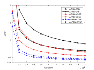
Figure 1: Simulation result of Example 1.

Example 2 (non-Guassian noise): In this example, we set the condition to be the same as in Example 1, except that the noise is distributed uniformly on $[-0.5,0.5]$. Then for the generated quaternion signals, the best possible qARMA predictor in hindsight will suffer an average error rate of 0.33. The simulation result is shown in Fig. 2. As we see, again the quaternion algorithms approach the optimal and outperform the non-quaternion algorithms.

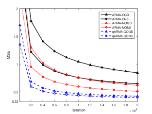
Figure 2: Simulation result of Example 2.

6 Conclusion

This paper proposed two online learning algorithms for the qARMA model. We transformed the learning problem of qARMA into a full information optimization task without explicit noise terms, and then extended online gradient descent and Newtons methods to the quaternion domain to solve the optimization problem. We further gave theoretical analyses and simulation examples to show the validity of this approach.

References

• [1] C. C. Took and D. P. Mandic, “The quaternion LMS algorithm for adaptive filtering of hypercomplex processes,” IEEE Trans. Signal Process., vol. 57, no. 4, pp. 1316-1327, Apr. 2009.
• [2] C. C. Took and D. P. Mandic, “A quaternion widely linear adaptive filter,” IEEE Trans. Signal Process., vol. 58, no. 8, pp. 4427-4431, Aug. 2010.
• [3] C. C. Took and D. P. Mandic, “Quaternion-valued stochastic gradient-based adaptive IIR filtering,” IEEE Trans. Signal Process., vol. 58, no. 7, pp. 3895-3901, Jul. 2010.
• [4] C. Jahanchahi and D. P. Mandic, “A class of quaternion Kalman filters,” IEEE Trans. Neural Netw. Learn. Syst., vol. 25, no. 3, pp. 533-544, Mar. 2014.
• [5] F. A. Tobar and D. P. Mandic, “Quaternion reproducing kernel Hilbert spaces: Existence and uniqueness conditions,” IEEE Trans. Inf. Theory, vol. 60, no. 9, pp. 5736-5749, Sep. 2014.
• [6] Y. Xia, C. Jahanchahi, and D. P. Mandic, “Quaternion-valued echo state networks,” IEEE Trans. Neural Netw. Learn. Syst., vol. 26, no. 4, pp. 663-673, Apr. 2015.
• [7] Y. Xia, C. Jahanchahi, T. Nitta, and D. P. Mandic, “Performance bounds of quaternion estimators,” IEEE Trans. Neural Netw. Learn. Syst., vol. 26, no. 12, pp. 3287-3292, Dec. 2015.
• [8] F. Shang and A. Hirose, “Quaternion neural-network-based PolSAR land classification in Poincare-sphere-parameter space,” IEEE Trans. Geosci. Remote Sens., vol. 52, no. 9, pp. 5693-5703, Sep. 2014.
• [9] D. Graupe, Time Series Analysis, Identification and Adaptive Filtering. Melbourne, FL: R.E. Krieger, 1984.
• [10] F. Ding, Y. Shi, and T. Chen, “Performance analysis of estimation algorithms of non-stationary ARMA processes,” IEEE Trans. Signal Process., vol. 54, no. 3, pp. 1041-1053, Mar. 2006.
• [11] J. Navarro-Moreno, “ARMA prediction of widely linear systems by using the innovations algorithm,” IEEE Trans. Signal Process., vol. 56, no. 7, pp. 3061-3068, Jun. 2008.
• [12] S. S. Pappas, et al, “Electricity demand loads modeling using AutoRegressive Moving Average (ARMA) models,” in Energy, vol. 33, no. 9, pp. 1353-1360, Sep. 2008.
• [13] S. Taylor, Modeling Financial Time Series. New York: Wiley, 1986.
• [14] O. Anava, E. Hzan, S. Mannor, and O. Shamir, “Online learning for time series prediction,” in Proc. JMLR, Workshop Conf. Proc. Conf. Learn. Theory., 2013, pp. 172-184.
• [15] C. Liu, S. C. Hoi, P. Zhao, and J. Sun, “Online ARIMA algorithms for time series prediction,” in Proc. 30th AAAI Conf. Artif. Intell., 2016, pp. 1867-1873.
• [16] M. Zinkevich, “Online convex programming and generalized infinitesimal gradient ascent,” in Proc. 20th Int. Conf. Mach. Learn., 2003, pp. 928-936.
• [17] E. Hazan, A. Agarwal, and S. Kale, “Logarithmic regret algorithms for online convex optimization,” Mach. Learn., vol. 69, no. 2-3, pp. 169-192, Oct. 2007.
• [18] T. A. Ell and S. J. Sangwine, “Quaternion involutions and anti-involutions,” Comput, Math. Applicat., vol. 53, no. 1, pp. 137-143, Jan. 2007.
• [19] C. C. Took and D. P. Mandic, “Augmented second-order statistics of quaternion random signals,” Signal Process., vol. 91, no. 2, pp. 214-224, Feb. 2011.
• [20] D. Xu, C. Jahanchahi, C. C. Took, and D. P. Mandic. (2014). “Quaternion derivatives: The GHR calculus.” [Online]. Available: http://arxiv.org/abs/1409.8168v1
• [21] D. Xu, Y. Xia, and D. P. Mandic, “Optimization in quaternion dynamic systems: Gradient, Hessian and learning algorithms,” IEEE Trans. Neural Netw. Learn. Syst., vol. 27, no. 2, pp. 249-261, Feb. 2016.
• [22] G. C. Goodwin and K. S. Sin, Adaptive Filtering, Prediction, and Control. Englewood Cliffs, NJ: Prentice-Hall, 1984.
• [23] Y. Huang and J. Benesty, Audio Signal Processing for Next Generation Multimedia Communication Systems. Boston, MA: Kluwer, 2004.
• [24] L. Rodman, Topics in Quaternion Linear Algebra. Princeton, NJ, USA: Princeton Univ. Press, 2014.
• [25] J. Wu, L. Zou, X. Chen, et al, “The estimation of eigenvalues of sum, difference, and tensor product of matrices over quaternion division algebra,” Linear Algebra Appl., vol. 428, no. 11-12, pp. 3023-3033, Jun. 2008.