Data-driven Computing in Elasticity
via Chebyshev Approximation

Abstract

This paper proposes a data-driven approach for computing elasticity by means of a non-parametric regression approach rather than an optimization approach. The Chebyshev approximation is utilized for tackling the material data-sets non-linearity of the elasticity. Also, additional efforts have been taken to compare the results with several other state-of-the-art methodologies.

I Introduction

In the era where machine learning is catapulting the conventional methodologies into the future, computational mechanics is a field where there was not much of development until recently. Data-driven solvers have become an emerging field lately due to its obvious advantages over conventional heuristic solvers. Data-driven solvers attempt to utilize the material data-set, without empirically modelling a constitutive law based on the stress-strain relation of the material, upon which the conventional methodologies of computational mechanics were heavily dependent on. Conventional approaches get the job done but are not good enough because of the unpredictable mapping between the equations and the real world behaviours of the systems. One cannot convert every possible real-time scenario into an appropriate equation. This calls for the need of Data-driven solvers that function based on real-time data rather than a set of heuristically created equations.

Elastic systems like shown in Fig. 1 (a), are easy to solve due to its linear nature by using Hooke’s law [1] while a system like shown in Fig. 1 (b) are inherently difficult to solve due to its non-linearity of stress-strain relationship even at infinitesimally small strains inputs. There are several models used for solving nonlinear elasticity namely Ramberg-Osgood [2], Hyperbolic law [3], Hardin-Drnevich [4], Duncan-Chang [5], Duncan-Selig [6] and the one that is commonly used is called Power law or also called as Ludwik’s law [7]. Check [19] for an extensive review. Even though the above-mentioned model capture the essence of nonlinear elasticity of the system to a certain degree, they are still a borderline approximation of the actual non-linearity. This is where date driven solvers like [8, 9, 10, 11, 12, 13, 14, 15, 16, 17, 18] become superior over the conventional methods mentioned earlier.

Section I provides a basic introduction about the research work, Section II explores and gives a detailed analysis of already existing literature and Section III gives a background knowledge of topics such as nonlinear elasticity and Chebyshev polynomials for a better understanding of the work. Section IV provides an in-depth knowledge of the experimental setup and the methodologies utilized. Finally Section V contains all the results obtained from the experiments and Section VI gives a strong closing statement by pressing on the importance of this work, the significance of the results obtained and future scope

II Related Works

Several methods like [8, 9] rely on minimizing the distance between a provided data set of the material and the subset of the appropriate stress-strain fields in equilibrium conditions. [8] considers the Mahalanobis distance [28] in order to incorporate the statistical uncertainty (2nd order) of data in computations. It is the distance between two groups’ multiple means (centroids) used in the analysis of discriminant. In [18], the method of minimizing the distance is extrapolated for nonlinearity in elasticity and Lagrange multipliers enforce the physical constraints. Data-driven solvers like [10], irrespective of the ideology of following a pure approach guided the given data in its entirety, heuristically adds a few constraints in order to develop a solver that is thermodynamically consistent during its solving phase. This directly contributes to fulfilling the second and first principles of thermodynamics which is independent of the experimental result’s quality. While most solvers lack generality due to its nature of the mathematical formulation, they fail at adapting themselves to new experimental data. This poses a real issue in real-time embedded applications as the solvers have to be remodelled periodically. [11] overcomes this downfall by directly connecting the data to computers for performing simulations. The so-performed numerical simulations will employ rules based on universal laws while minimizing the need for specifically engineered models by making use of manifold learning [29] methodologies.

III Background

III-A Nonlinear Elasticity

In order to understand nonlinear elasticity in detail, it becomes vital to have a basic understanding of elasticity in general. The key pillars for a material to be elastic in nature are – when the application of the load is stopped, the deformation vanishes, the deformation is independent of its history and the potential-energy exist as a function of deformation. When a material satisfies the above criteria for elasticity and its stress-strain relation is nonlinear like in Fig. 1 (b), then they are called as nonlinear elastic materials.

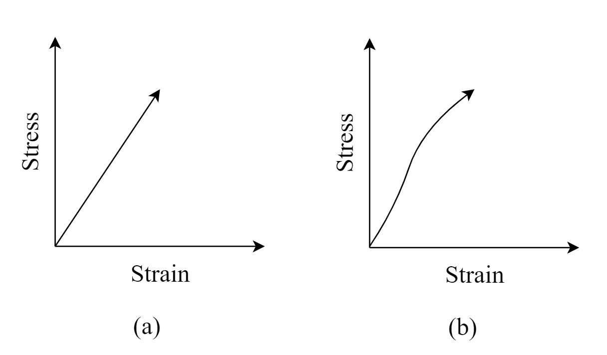
Figure 1: Stress-strain relation graphs of (a) Linearly Elastic and (b) Non-linearly elastic systems.

This nonlinearity between the stress and strain is exactly the hurdle that prevents conventional methodologies from functioning at their fullest and makes it hard to map to a set of predefined equations.

III-B Chebyshev Polynomials

Chebyshev polynomials play a vital role in approximation theory [20] due to its roots of the Chebyshev polynomials of the first kind and are also known as Chebyshev nodes [21]. During the polynomial interpolation, these nodes are used. As a result, the resulting polynomial of interpolation reduces the problem of Runge’s phenomenon. It also delivers an approximation that is extremely near to the optimum approximation polynomial to a function that is continuous under the maximum norm. This approximation inherently leads to the Clenshaw–Curtis quadrature method [22].

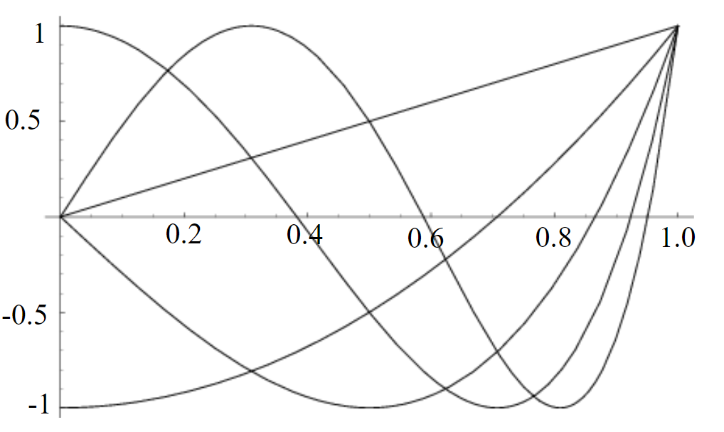
Figure 2: Illustration of The Chebyshev polynomials of the first kind ${T_{n}}\left(x\right)$ for $x\in\left[{0,1}\right]$ and $n=1,2,\ldots,5$.

The Chebyshev polynomials of the first kind ${T_{n}}\left(x\right)$ are illustrated in Fig. 2 for $x\in\left[{0,1}\right]$ and $n=1,2,\ldots,5$. Using a Chebyshev Polynomial of the First Kind $T$, we can define

$${{c}_{j}} \equiv\frac{2}{N}\sum\limits_{k=1}^{N}{f\left({{x}_{k}}\right)}{{T}_{j}}\left({{x}_{k}}\right)$$ (1)

$$=\frac{2}{N}\sum\limits_{k=1}^{N}{f\left[\cos\left\{\frac{\pi\left(k-\frac{1}{2}\right)}{N}\right\}\right]}\cos\left\{\frac{\pi j\left(k-\frac{1}{2}\right)}{N}\right\}$$ (1)

where, $k=1,2,\ldots,n$. Then,

$$f\left(x\right)\approx\sum\limits_{k=0}^{N-1}{{{c}_{k}}{{T}_{k}}\left(x\right)}-\frac{1}{2}{{c}_{0}}$$

For the $N$ zeros of ${T_{N}}\left(x\right)$ it is exact and this way of approximation is essential because, in case of truncation, the error is distributed evenly and smoothly over $\left[{-1,1}\right]$. The Chebyshev approximation [23, 30] is very near to the Minimax Polynomial.

IV Experiments

IV-A Experimental Setup

We use MATLAB as the test platform and take advantage of chebfun [27] package for carrying out calculations of Chebyshev approximation. For exponentially increasing the agility of processing of data, a computer with Intel Core i7-6700HQ Skylake CPU running at 2.60Hz and a DDR4 16 GB ram memory. The truss configuration used for the results shown in this paper is illustrated in Fig. 6 but the methodology can be extended to any truss configuration. GitHub Repository for all the codes used in this paper: https://github.com/rahulvigneswaran/Data-Driven-Computing-in-Elasticity-via-Chebyshev-Approximation

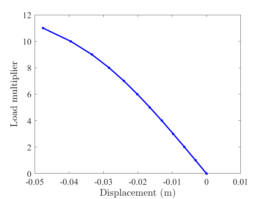
(a)

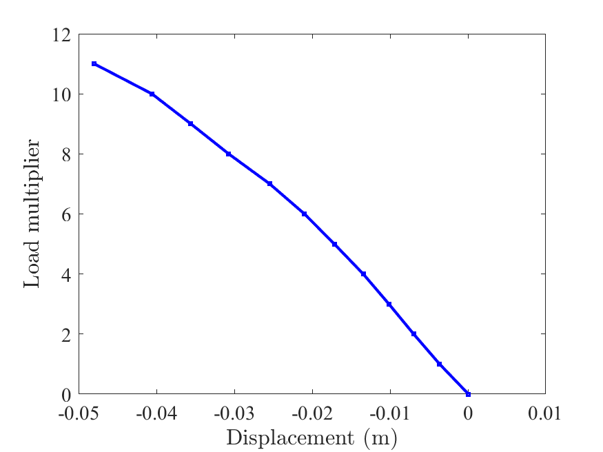
(b)

Figure 3: Obtained paths of equilibrium by varying load multiplier: (a) Method proposed in this paper; (b) Method proposed in [26].

(a)

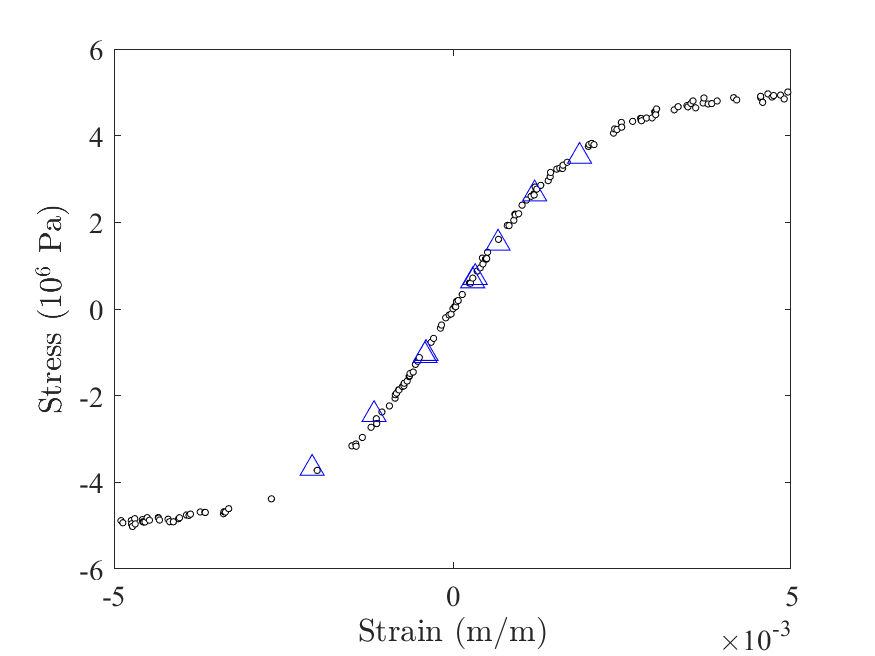
(b)

Figure 4: Solutions obtained for the load multiplier $\lambda=10$: (a) Method proposed in this paper; (b) Method proposed in [26].

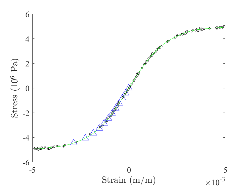
(a)

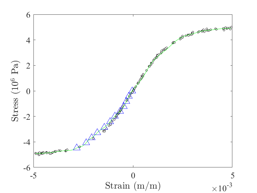
(b)

Figure 5: Obtained stress-strain pairs of member (A). (a) The proposed method and (b) Method from [24] applied to the formulation in [14]. $\bigcirc\to$ material data point, $\Delta\to$ obtained strain-stress pair.

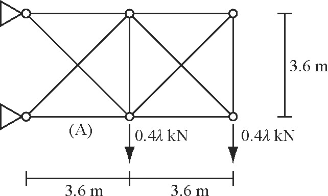
Figure 6: 10-bar truss configuration [26]

IV-B Methodology

Even though this methodology can be extended to any nonlinear elasticity problem unlike [24], for the purpose of simplicity, we have limited our explanation to the scenario of truss undergoing small deformations. This problem when formulated like in [15], inherently becomes a nonconvex optimization [25] problem. In this paper, we have utilized the method used in [26], which proposes a novel method by converting the problem into a set of nonlinear equations that can be solved easily.

The compatibility conditions and the force balance relations are as follows,

$$\begin{gathered}{\varepsilon_{i}}=b_{i}^{T}u\\ \sum\limits_{i=1}^{m}{{\upsilon_{i}}{\sigma_{i}}{b_{i}}}=p\\ \end{gathered}$$

where, ${\varepsilon_{i}}$ is axial strain, ${{\sigma_{i}}}$ is axial stress and $\upsilon_{i}$ is the volume of the member $i(i=1,2,\ldots,m)$ respectively. In equation (IV-B), $b_{1},b_{2},\ldots,b_{m}$ are constant vectors. Lets suppose the material dataset has been provided and is represented as $D=\left\{{\left({{{\overset{\lower 5.0pt\hbox{$\smash{\scriptscriptstyle\smile}$}}{\varepsilon}}_{1}},{{\overset{\lower 5.0pt\hbox{$\smash{\scriptscriptstyle\smile}$}}{\sigma}}_{1}}}\right),\ldots,\left({{{\overset{\lower 5.0pt\hbox{$\smash{\scriptscriptstyle\smile}$}}{\varepsilon}}_{d}},{{\overset{\lower 5.0pt\hbox{$\smash{\scriptscriptstyle\smile}$}}{\sigma}}_{d}}}\right)}\right\}$ where, the observed uniaxial strains and stresses are denoted by ${{{\overset{\lower 5.0pt\hbox{$\smash{\scriptscriptstyle\smile}$}}{\varepsilon}}_{j}}}$ and ${{{\overset{\lower 5.0pt\hbox{$\smash{\scriptscriptstyle\smile}$}}{\sigma}}_{j}}}$ respectively. For each member $i$, the stress estimated $(S_{i})$, for a given ${{\varepsilon_{i}}}$ is calculated by using the kernel regression [31] in [26] using the Gaussian kernel of the following form,

$${s_{i}}=\frac{{\sum\limits_{j=1}^{d}{\exp\left[{-\alpha{{\left({{\varepsilon_{i}}-{{\overset{\lower 5.0pt\hbox{$\smash{\scriptscriptstyle\smile}$}}{\varepsilon}}_{j}}}\right)}^{2}}}\right]}{{\overset{\lower 5.0pt\hbox{$\smash{\scriptscriptstyle\smile}$}}{\sigma}}_{j}}}}{{\sum\limits_{j=1}^{d}{\exp\left[{-\alpha{{\left({{\varepsilon_{i}}-{{\overset{\lower 5.0pt\hbox{$\smash{\scriptscriptstyle\smile}$}}{\varepsilon}}_{j}}}\right)}^{2}}}\right]}}}$$

where, $\alpha>0$ is acquired by cross validation of D. A data-driven solving approach can be formulated as,

$$minimize\left\|{\sigma-s}\right\|$$

with constraints (IV-B) and (IV-B). Here, equation (IV-B) in conjunction with the given material data, is basically used as a lookup table but the drawback is that the equation (IV-B) has to be calculated every time the material data has to be referred by the algorithm.

In this paper, we have experimented by replacing the equation (IV-B), that is, the Kernel regression with Chebyshev approximation (Equation (III-B)). The advantage is that, by doing so, we create a one-time smooth data curve from the given coarse experimental data which can be accessed easily like simple function $f(x)$ where $x$ is the input strain and $f(x)$ will provide the corresponding stress output.

V Results

An extensive comparison has been carried out for better assessment of the results. Fig. 7 is the stress-strain relation of the material that is considered for the assessment. It is evident from it that the dataset is coarse in nature. The obtained equilibrium paths of the method proposed in [26] and this paper are depicted in Fig. 3. The solutions obtained for the load multiplier $\lambda=10$ are shown in Fig. 4. The obtained stress-strain pairs of member (A) in the truss (Fig. 6) are shown in Fig. 5.

Table I: Computational Costs

Formulation	Solving Process	Time (s)
Proposed Method	Chebyshev Approx.	0.3
	Nonlinear Eqn.	3.2
	Total	3.5
Kernal Regression [26]	Cross Validation	2.3
	Nonlinear Eqn.	2.64
	Total	7.18
Formulation in [14]	MIP [24]	309.4
Formulation in [14]	Heuristic [14]	0.6
Formulation in [15]	NLP	13.8

Table I compares the computation time of the proposed method with methods proposed in [14, 15, 24, 16]. It is evident from the result that the proposed method has significantly outperformed the previously proposed state-of-the-art model by $51.3\%$. Even though the model proposed in [14] has a very low computation time compared to other models, it is heuristically designed. It does not necessarily yield an optimal solution. For example, for a load multiplier of 10, the value of the solution is 1.316 J, while the actual solution is 0.251 J. Thus, having 81% deviation from the actual solution, proving that the heuristic converged an inexact solution, irrespective of that fact that it is computationally cheap. As a result, the method proposed in this paper has a significant advantage over the existing models, making it suitable for the application of nonlinear elasticity. A much more extensive analysis with varying load multipliers have been done and can be viewed at https://rahulvigneswaran.github.io/Data-Driven-Computing-in-Elasticity-via-Chebyshev-Approximation/.

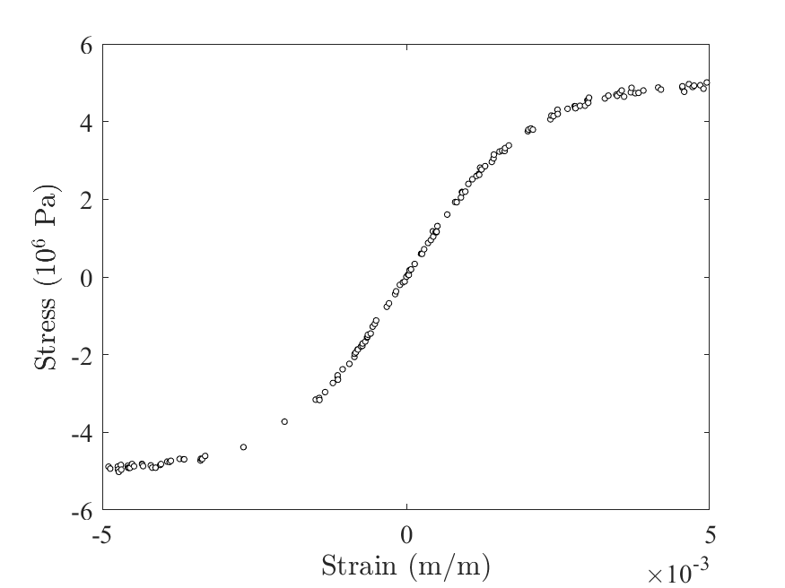
Figure 7: Material dataset used for the experiments.

VI Conclusion

The same experiment was carried out several other algorithms including neural network based curve-fitting which showed significantly faster results compared to Chebyshev approximation. Yet, they were not considered as suitable candidates due to its inherent nature that requires it to fit a curve, which might become time consuming when the distribution of the data is sparse and the curve that is fit becomes increasingly erroneous and might not necessarily mimic the behaviour of the actual system while Chebyshev approximation can handle it with ease.

From the results, it becomes evident that the proposed methodology is significantly faster than the existing cutting edge models while preserving the generality approach in elasticity. As we can define the linear elasticity as a special subset of nonlinear elasticity, the proposed method holds good for both linear and nonlinear elastic cases, making it a universal solver for elastic bodies. Deep learning [34] has shown its effectiveness in many of the emerging fields ([32, 33]) which were traditionally completely based on heuristic methods. Therefore, using Deep learning in conjunction with the methodology proposed in this paper can be considered as a future endeavour.

References

- [1] Rychlewski, J., 1984. On Hooke’s law. Journal of Applied Mathematics and Mechanics, 48(3), pp.303-314.
- [2] Ramberg, W. and Osgood, W.R., 1943. Description of stress-strain curves by three parameters.
- [3] Keyfitz, B.L. and Kranzer, H.C., 1980. A system of non-strictly hyperbolic conservation laws arising in elasticity theory. Archive for Rational Mechanics and Analysis, 72(3), pp.219-241.
- [4] Fahey, M. and Carter, J.P., 1993. A finite element study of the pressuremeter test in sand using a nonlinear elastic plastic model. Canadian Geotechnical Journal, 30(2), pp.348-362.
- [5] Huang, B., Bathurst, R.J. and Hatami, K., 2009. Numerical study of reinforced soil segmental walls using three different constitutive soil models. Journal of Geotechnical and Geoenvironmental engineering, 135(10), pp.1486-1498.
- [6] Katona, M.G., 2015. Influence of soil models on performance of buried culverts (No. 15-0560).
- [7] Isselin, J., Iost, A., Golek, J., Najjar, D. and Bigerelle, M., 2006. Assessment of the constitutive law by inverse methodology: Small punch test and hardness. Journal of Nuclear Materials, 352(1-3), pp.97-106.
- [8] Ayensa-Jiménez, J., Doweidar, M.H., Sanz-Herrera, J.A. and Doblaré, M., 2018. A new reliability-based data-driven approach for noisy experimental data with physical constraints. Computer Methods in Applied Mechanics and Engineering, 328, pp.752-774.
- [9] Conti, S., Müller, S. and Ortiz, M., 2018. Data-driven problems in elasticity. Archive for Rational Mechanics and Analysis, pp.1-45.
- [10] González, D., Chinesta, F. and Cueto, E., 2019. Thermodynamically consistent data-driven computational mechanics. Continuum Mechanics and Thermodynamics, 31(1), pp.239-253.
- [11] Ibanez, R., Abisset-Chavanne, E., Aguado, J.V., Gonzalez, D., Cueto, E. and Chinesta, F., 2018. A manifold learning approach to data-driven computational elasticity and inelasticity. Archives of Computational Methods in Engineering, 25(1), pp.47-57.
- [12] Ibañez, R., Borzacchiello, D., Aguado, J.V., Abisset-Chavanne, E., Cueto, E., Ladevèze, P. and Chinesta, F., 2017. Data-driven non-linear elasticity: constitutive manifold construction and problem discretization. Computational Mechanics, 60(5), pp.813-826.
- [13] Kanno, Y., 2018. Simple heuristic for data-driven computational elasticity with material data involving noise and outliers: a local robust regression approach. Japan Journal of Industrial and Applied Mathematics, 35(3), pp.1085-1101.
- [14] Kirchdoerfer, T. and Ortiz, M., 2016. Data-driven computational mechanics. Computer Methods in Applied Mechanics and Engineering, 304, pp.81-101.
- [15] Kirchdoerfer, T. and Ortiz, M., 2017. Data driven computing with noisy material data sets. Computer Methods in Applied Mechanics and Engineering, 326, pp.622-641.
- [16] Latorre, M. and Montáns, F.J., 2018. Experimental data reduction for hyperelasticity. Computers & Structures.
- [17] Leygue, A., Coret, M., Réthoré, J., Stainier, L. and Verron, E., 2018. Data-based derivation of material response. Computer Methods in Applied Mechanics and Engineering, 331, pp.184-196.
- [18] Nguyen, L.T.K. and Keip, M.A., 2018. A data-driven approach to nonlinear elasticity. Computers & Structures, 194, pp.97-115.
- [19] Zeidler, E., 1988. Basic Equations of Nonlinear Elasticity Theory. In Nonlinear Functional Analysis and its Applications (pp. 158-232). Springer, New York, NY.
- [20] Butzer, P.L. and Nessel, R.J., 1971. Fourier analysis and approximation, Vol. 1. Reviews in Group Representation Theory, Part A (Pure and Applied Mathematics Series, Vol. 7).
- [21] Adibi, H. and Assari, P., 2010. Chebyshev wavelet method for numerical solution of Fredholm integral equations of the first kind. Mathematical problems in Engineering, 2010.
- [22] Gentleman, W.M., 1972. Implementing Clenshaw-Curtis quadrature, II computing the cosine transformation. Communications of the ACM, 15(5), pp.343-346.
- [23] Ames, W.F. and Brezinski, C., 1993. Numerical recipes in Fortran (The art of scientific computing): WH Press, SA Teukolsky, WT Vetterling and BP Flannery, Cambridge Univ. Press, Cambridge, 1992. 963 pp., US $49.95, ISBN 0-521-43064-X.
- [24] Kanno, Y., 2018. Mixed-integer programming formulation of a data-driven solver in computational elasticity. Optimization Letters, pp.1-10.
- [25] Jain, P. and Kar, P., 2017. Non-convex optimization for machine learning. Foundations and Trends® in Machine Learning, 10(3-4), pp.142-336.
- [26] Kanno, Y., 2018. Data-driven computing in elasticity via kernel regression. Theoretical and Applied Mechanics Letters, 8(6), pp.361-365.
- [27] Driscoll, T.A., Hale, N. and Trefethen, L.N., 2014. Chebfun guide.
- [28] De Maesschalck, R., Jouan-Rimbaud, D. and Massart, D.L., 2000. The mahalanobis distance. Chemometrics and intelligent laboratory systems, 50(1), pp.1-18.
- [29] Wang, J., Zhang, Z. and Zha, H., 2005. Adaptive manifold learning. In Advances in neural information processing systems (pp. 1473-1480).
- [30] Mohan, N. and Soman, K.P., 2018, February. Power system frequency and amplitude estimation using variational mode decomposition and chebfun approximation system. In 2018 Twenty Fourth National Conference on Communications (NCC)(pp. 1-6). IEEE.
- [31] Bishop, C.M., 2006. Pattern recognition and machine learning. springer.
- [32] Rahul-Vigneswaran K, Vinayakumar R, Soman KP and Prabaharan Poornachandran. Evaluating Shallow and Deep Neural Networks for Network Intrusion Detection Systems in Cyber Security. In 2018 9th International Conference on Computing, Communication and Networking Technologies (ICCCNT) (pp. 1-6). IEEE.
- [33] Rahul-Vigneswaran K, Prabhaharan Poornachandran and Soman KP. A Compendium on Network and Host Based Intrusion Detection Systems. In 2019 International Conference on Data Science, Machine learning & Applications (ICDSMLA) (pp. 1-8). Springer
- [34] LeCun, Y., Bengio, Y. and Hinton, G., 2015. Deep learning. nature, 521(7553), p.436.