Pulsating in unison at optical and X-ray energies: simultaneous high-time resolution observations of the transitional millisecond pulsar PSR J1023+0038

Abstract

PSR J1023+0038 is the first millisecond pulsar discovered to pulsate in the visible band; such a detection took place when the pulsar was surrounded by an accretion disk and also showed X-ray pulsations. We report on the first high time resolution observational campaign of this transitional pulsar in the disk state, using simultaneous observations in the optical (TNG, NOT, TJO), X-ray (XMM-Newton, NuSTAR, NICER), infrared (GTC) and UV (Swift) bands. Optical and X-ray pulsations were detected simultaneously in the X-ray high intensity mode in which the source spends $\sim 70\%$ of the time, and both disappeared in the low mode, indicating a common underlying physical mechanism. In addition, optical and X-ray pulses were emitted within a few km, had similar pulse shape and distribution of the pulsed flux density compatible with a power-law relation $F_{\nu}\propto\nu^{-0.7}$ connecting the optical and the 0.3–45 keV X-ray band. Optical pulses were detected also during flares with a pulsed flux reduced by one third with respect to the high mode; the lack of a simultaneous detection of X-ray pulses is compatible with the lower photon statistics. We show that magnetically channeled accretion of plasma onto the surface of the neutron star cannot account for the optical pulsed luminosity ($\sim 10^{31}$ erg s^-1). On the other hand, magnetospheric rotation-powered pulsar emission would require an extremely efficient conversion of spin-down power into pulsed optical and X-ray emission. We then propose that optical and X-ray pulses are instead produced by synchrotron emission from the intrabinary shock that forms where a striped pulsar wind meets the accretion disk, within a few light cylinder radii away, $\sim 100$ km, from the pulsar.

1 Introduction

Transitional millisecond pulsars are fast spinning, weakly magnetic ($B_{*}\approx 10^{8}$ G) neutron stars (NSs) with a low mass ($\lower 2.15277pt\hbox{$\;\buildrel<\over{\sim}\;$}M_{\odot}$) companion star, that undergo transitions between distinct emission regimes over a timescale of less than a couple of weeks. During bright X-ray outbursts ($L_{X}\lower 2.15277pt\hbox{$\;\buildrel>\over{\sim}\;$}10^{36}$ erg s^-1) they behave like accreting millisecond pulsars (Wijnands & van der Klis 1998; see Patruno & Watts 2012; Campana & Di Salvo 2018 for reviews), which accrete matter transferred by the donor through a disk and emit X-ray pulsations due to the channeling of the plasma in-flow onto the magnetic poles. When accretion stops ($L_{X}\lower 2.15277pt\hbox{$\;\buildrel<\over{\sim}\;$}10^{32}$ erg s^-1) they behave as redback pulsars (D’Amico et al., 2001; Roberts et al., 2018); the rotation of the NS magnetic field powers both radio and high energy (X-rays, gamma-rays) pulsed emission, and a relativistic wind that shocks off the matter transferred by the companion close to the inner Lagrangian point of the binary, and ejects it from the system (see, e.g., Burderi et al., 2001). IGR J18245–2452/PSR M28-I performed a clear transition between these two regimes in 2013 (Papitto et al., 2013; Ferrigno et al., 2014).

State transitions from two more millisecond pulsars have been observed, so far, PSR J1023+0038 (Archibald et al., 2009; Stappers et al., 2014; Patruno et al., 2014) and XSS J12270-4859 (de Martino et al., 2010, 2013; Bassa et al., 2014). However, the accretion disk state of these sources was peculiar, it lasted almost a decade and had an X-ray luminosity much lower ($L_{X}\simeq 5\times 10^{33}$ erg s^-1) than that usually shown by low mass X-ray binaries (Linares, 2014). The X-ray light curve repeatedly showed transitions on a time scale of $\sim 10$ s between two intensity modes characterized by a definite value of the luminosity; these were dubbed high ($L_{X}\simeq 7\times 10^{33}$ erg s^-1) and low ($L_{X}\simeq 10^{33}$ erg s^-1) modes (Bogdanov et al., 2015; Campana et al., 2016). X-ray flares reaching up to a few times $10^{34}$ erg s^-1 were also observed. Coherent X-ray pulsations were detected only during the high mode (Archibald et al., 2015; Papitto et al., 2015) and interpreted in terms of magnetically channeled accretion onto the magnetic poles, even though the low X-ray luminosity at which they were observed should not allow matter to overcome the centrifugal barrier due to pulsar rotation (but see also Bozzo et al., 2018). Moreover, the spin-down rate of PSR J1023+0038 during the disk state (Jaodand et al., 2016, J16 in the following) was close to the value taken during the rotation-powered radio pulsar state and its modulus is lower by at least one order of magnitude than that expected if accretion or propeller ejection of matter takes place. A relatively bright continuous radio emission with a flat spectral shape was detected and interpreted as compact self-absorbed synchrotron jet (Deller et al., 2015), with radio flares occurring during the X-ray low mode indicating ejection of optically thin plasmoid (Bogdanov et al., 2018). Flares and flickering reminiscent of the high/low mode transitions were also seen in the optical (Shahbaz et al., 2015; Papitto et al., 2018; Kennedy et al., 2018) and in the infrared (Hakala & Kajava, 2018; Shahbaz et al., 2018) bands; the optical light was polarized at a $\sim 1\%$ degree (Baglio et al., 2016), to a different extent during the various modes (Hakala & Kajava, 2018). The appearance of a disk in transitional millisecond pulsars in such a sub-luminous state was also accompanied by a factor of a few increase in the GeV gamma-ray luminosity (Torres et al., 2017), while only upper limit were placed on the TeV flux (Aliu et al., 2016).

This complex phenomenology led to a flurry of different interpretations either based on the emission of a rotation powered pulsar enshrouded by disk matter (Takata et al., 2014; Coti Zelati et al., 2014; Li et al., 2014), a pulsar that propels away disk matter (Papitto et al., 2014; Papitto & Torres, 2015) or a pulsar accreting mass at a very low rate from disk trapped near corotation (D’Angelo & Spruit, 2012). The possibility that switching between the high and the low X-ray modes marked changes between a radio pulsar and a propeller regime was also proposed (Linares, 2014; Campana et al., 2016; Coti Zelati et al., 2018).

Recently, Ambrosino et al. (2017) discovered optical pulsations at the spin period of PSR J1023+0038, produced by a region a few tens of km away from the NS. This finding was interpreted by the authors as a strong indication that a rotation-powered pulsar was active in the system, even when the accretion disk was present. In fact, the pulsed luminosity observed in the visible band was too large to be produced by reprocessing of accretion-powered X-ray emission or cyclotron emission by electrons in the accretion columns above the pulsar polar caps. Here we report on the first high time resolution multi-wavelength observational campaign of PSR J1023+0038 in the disk state aimed at exploring the relation between optical and X-ray pulses, and their properties in the different intensity modes. The campaign was performed on May 23-24, 2017 and involved simultaneous high time resolution observations by: the fast optical photometer SiFAP mounted at the INAF Telescopio Nazionale Galileo (TNG), X-ray instruments on-board XMM-Newton and NuSTAR, and the Canarias InfraRed Camera Experiment (CIRCE) at the Gran Telescopio Canarias (GTC). Optical, UV and X-ray spectra and images were also obtained thanks to Nordic Optical Telescope (NOT), Telescopi Joan Oró (TJO) and Neil Gehrel’s Swift Observatory observations. Further high time resolution optical observations were performed by TNG/SiFAP on December 20, 2017, and were analyzed with observations performed by the X-ray NICER mission a few weeks earlier.

2 Observations

Tab. 1 lists the observations analyzed and discussed in this paper, we give details on the analysis of the different data sets in the following.

Table 1: Log of the observations of PSR J1023+0038

Telescope/Instrument	MJD start time	Exposure (s)	Band	Mode/Magnitude
2017 May 23
NuSTAR/FPMA-FPMB	57896.035995	82514.0	3–79 keV
Nordic Optical Telescope/ALFOSC	57896.896694	3600.0	440–695 nm	grism#19
XMM-Newton/MOS1 (XMM1)	57896.905272	24651.7	0.3–10 keV	Small window
XMM-Newton/MOS2 (XMM1)	57896.905765	24613.9	0.3–10 keV	Small window
Telescopi Joan Oró/MEIA2	57896.907924	300.0	Johnson-V	$16.85\pm 0.01$
Swift/UVOT	57896.915625	1710.7	UVW1	Imaging+Event
Swift/XRT	57896.915579	1721.6	0.3–10 keV	Photon counting
XMM-Newton/EPIC-pn (XMM1)	57896.929398	24914.0	0.3–10 keV	Timing
GTC/CIRCE	57896.930555	4800.0	Ks	Fast imaging
TNG/SiFAP (TNG1)	57896.970058	3297.7	white filter	Fast timing
2017 May 24
XMM-Newton/EPIC-pn (XMM2)	57897.739274	23413.0	0.3–10 keV	Timing
XMM-Newton/MOS1 (XMM2)	57897.715133	23150.6	0.3–10 keV	Small window
XMM-Newton/MOS2 (XMM2)	57897.715642	23112.8	0.3–10 keV	Small window
TNG/SiFAP (TNG2)	57897.890802	8397.2	white filter	Fast timing
Telescopi Joan Oró/MEIA2	57897.896660	600.0	U-Johnson	$18.1\pm 0.1$
Telescopi Joan Oró/MEIA2	57897.903954	200.0	B-Johnson	$17.10\pm 0.03$
Telescopi Joan Oró/MEIA2	57897.906622	200.0	V-Johnson	$16.64\pm 0.02$
Telescopi Joan Oró/MEIA2	57897.909287	200.0	R-Cousins	$16.31\pm 0.02$
Telescopi Joan Oró/MEIA2	57897.911955	200.0	I-Cousins	$15.91\pm 0.02$
2017 December 2–20
NICER (1034060101)	58089.019028	3070.0	0.2–12 keV
NICER (1034060102)	58090.044676	1963.0	0.2–12 keV
NICER (1034060103)	58093.393750	1144.0	0.2–12 keV
TNG/SiFAP (TNG3-B)	58107.126433	3298.3	Johnson-B	Fast timing
TNG/SiFAP (TNG3-V)	58107.179563	3298.3	Johnson-V	Fast timing
TNG/SiFAP (TNG3-R)	58107.235471	3298.3	Johnson-R	Fast timing

2.1 X-ray observations

2.1.1 XMM-Newton/EPIC

We analyzed XMM-Newton Target of Opportunity (ToO) observations of PSR J1023+0038 performed on 2017, May 23 (Id. 0794580801, XMM1 in the following) and May 24 (Id. 0794580901, XMM2 in the following) in the Discretionary Time of the Project Scientist (PIs: Papitto, Stella). We used the SAS (Science Analysis Software) v.16.1.0 to reduce the data. We transformed the photon arrival times observed by XMM-Newton as if they were observed at the line of nodes of the Solar System barycenter using the source position derived by Deller et al. (2012), RA=10:23:47.687198(2), DEC=00:38:40.84551(4), the JPL ephemerides DE405 and the barycen tool. We used the same parameters to correct arrival times observed by other instruments considered in this paper. We discarded the first 3.5 ks of XMM1 data from the analysis because high flaring particle background – apparent from the 10-12 keV light curve – contaminated data and prevented identification of X-ray modes. In both observations the EPIC-pn was operated with a time resolution of 29.5 $\mu$s (timing mode) and a thin optical blocking filter. We defined source and background regions with coordinates RAWX=27–47 and RAWY=3–5, respectively, and retained good events characterized by a single or a double pattern. EPIC MOS1 and MOS2 cameras observed the target in small window mode with a time resolution of 0.3 s, and a thin optical blocking filter. We extracted source photons falling within a circular region centered on the source position with a 35^′′radius, and background photons from a 100^′′-wide, source-free circular region of one of the outer CCDs; we retained good events with patterns as complex as quadruples. We created background-subtracted light curves with the task epiclccorr. Redistribution matrices and ancillary response files were computed using rmfgen and arfgen, and the spectra re-binned to have at least 25 counts per bin and no more than three bins per resolution element in the 0.3–10 keV energy band.

2.2 NuSTAR

We analyzed the NuSTAR ToO observation of PSR J1023+0038 performed on 2017, May 23 (Id. 80201028002, starting at 00:26:09 UTC and lasting 160 ks, for a total exposure time of 82.5 ks; PI: Papitto). We reduced the observation by performing standard screening and filtering of the events with the NuSTAR data analysis package (NUSTARDAS) version v.1.8.0 with CALDB 20170126. We selected source and background events from circular regions of 55^′′radius centered at the source location and in a source-free region away from the source, respectively.

2.3 NICER

We present the analysis of NICER observations of PSR J1023+0038 performed on 2017, December 2 (Id. 1034060101), December 3 (Id. 1034060102) and December 6 (Id. 1034060103). The events across the 0.2-12 keV band (Gendreau et al., 2012) were processed and screened using the HEASOFT version 6.24 and NICERDAS version 4.0.

2.4 Swift/XRT

We consider the Swift observations of PSR J1023+0038 that started on 2017, May 23 at 21:53 (UT, Id. 00033012149) with an exposure of 1.7 ks. We reduced data obtained with the X-ray Telescope (XRT) in Photon Counting mode using the HEASoft tool xrtpipeline, extracted light curves and spectra with xselect from a circle with a 47^′′radius centered on the source position, and produced ancillary response files using xrtmkarf. The XRT observed a variable count rate between 0.05 and 0.4 s^-1. The 0.3–10 keV spectrum could be described by an absorbed power law with absorption column fixed $N_{H}=5\times 10^{20}$ cm^-2 and photon index $\Gamma=1.6\pm 0.2$, giving an unabsorbed 0.3–10 keV flux of $(1.0\pm 0.1)\times 10^{-11}$ erg cm^-2 s^-1, typical for the disk state of PSR J1023+0038.

2.5 Optical/UV observations

2.6 TNG

We observed PSR J1023+0038 with the SiFAP fast optical photometer (Meddi et al., 2012; Ambrosino et al., 2016, 2017) mounted at the 3.6 m TNG starting on 2017, May 23 at 23:17 (TNG1, overlapping for 3.0 ks with XMM1), on 2017, May 24 at 21:21 (TNG2, overlapping for 8.0 ks with XMM2), and on 2017, December 20 at 03:02 (TNG3). The three observations were performed during the Director discretionary time. We observed PSR J1023+0038 using the channel of SiFAP that ensured the maximum possible time resolution (25 ns), and a $V=15.6$ mag reference star UCAC4 454-048424 (Zacharias et al., 2013) with the second channel which operated with a time resolution of 1 ms during TNG1, and 5 ms during TNG2 and TNG3. The size of the on-source channel of SiFAP is $0.13\times 0.13\,cm^{2}$ which at the $F/11$ focus of the TNG corresponds to nearly $7\times 7\,$arcsec². In TNG1 and TNG2 we used a white filter covering the 320–900 nm band and maximum between 400 and 600 nm (i.e. roughly corresponding to the B and V Johnson filters, see Supplementary Fig.1 in Ambrosino et al. 2017). During TNG3 we observed the source with Johnson B ($\lambda_{eff}=445$ nm, $\Delta\lambda_{FWHM}=94$ nm), V ($\lambda_{eff}=551$ nm, $\Delta\lambda_{FWHM}=88$ nm) and R ($\lambda_{eff}=658$ nm, $\Delta\lambda_{FWHM}=138$ nm) filters, for 3.3 ks each; filters could not be used on the reference star due to problems with the instrumental set-up . We estimated the background by tilting the pointing direction of the telescope by a few tens of arcseconds for $\sim 100$ s; this was done four times during TNG2 (roughly every half an hour) and once during TNG1 (at the end of the exposure) and during each of the three filtered observations of TNG3. The background count rate increased during TNG2 as the elevation of the source over the horizon decreased and the contamination by diffuse light was correspondingly larger; we then evaluated the background contribution by fitting the count rate observed during the four intervals with a quadratic polynomial. During TNG1 the background was estimated only at the end of the exposure, and considering that its contribution increases as the source declines over the horizon, it is almost certainly larger than the actual value that affected the observation of the source.

The SiFAP clock showed drifts with respect to the actual time measured by two Global Positioning System (GPS) pulse-per-second (PPS) signals that were used to mark the start and the stop times of each observation. For this reason the total elapsed time by the clock exceeded the GPS time by $\Delta t_{SiFAP}-\Delta t_{GPS}=0.84$ and $4.23$ ms during TNG1 and TNG2, each lasting $\Delta t_{GPS}=3300.0$ and 8400.0 s, respectively. During TNG3, the SiFAP clock lagged the GPS signal by $3.89$, $3.13$ and $3.08$ ms during the exposures with B, V and R filters, respectively, each lasting $\Delta t_{GPS}=3300.0$ s. As no further information on the dependence of the drift on the various parameters that affect the photometer operations (e.g. temperature, count rate) is available, the best possible guess is that the drift rate was constant. Following Ambrosino et al. (2017), we corrected the arrival times recorded by SiFAP using the relation $t_{arr}=t_{SiFAP}\times(\Delta t_{GPS}/\Delta t_{SiFAP})$. Subsequently we used the software tempo2 (Hobbs et al., 2006) to correct the photon arrival times to the Solar System barycenter, using the position of PSR J1023+0038 reported in Sec. 2.1.1 and the geocentric location of the TNG (X=5327447.481, Y=-1719594.927, Z=3051174.666), along with the JPL ephemerides DE405. During the 3.3 ks exposure of TNG1 we measured an average count rate of $\sim 2.59\times 10^{4}$, $3.70\times 10^{4}$ and $1.75\times 10^{4}$ s^-1 from the source, the reference star and the sky background, respectively. Values of $2.95\times 10^{4}$, $4.19\times 10^{4}$ and $1.11\times 10^{4}$ s^-1 were measured for the same quantities during TNG2.

2.7 XMM-Newton/OM

The Optical Monitor (OM) on-board XMM-Newton observed the source during XMM1 and XMM2 with a B filter ($\lambda_{eff}=450$ nm) and using the fast mode, which has a time resolution of 0.5 s. We extracted source photons from a 6-pixel wide circle (corresponding to 2.9 arcsec) and background from an annulus with inner and outer radius of 7.2 and 9.9 pixel, respectively. Observed count rates, $R_{OM}$, were converted to flux and magnitude units using the relations $f_{\lambda}=1.29\times 10^{-16}\,R_{OM}$ erg cm^-2 s^-1 Å^-1 and $mag=19.266-2.5\log_{10}R_{OM}$.

2.8 Swift/UVOT

The Ultraviolet Optical Telescope (UVOT) on-board Swift observed PSR J1023+0038 with the UVW1 filter ($\lambda_{c}=260$ nm) for 674.1 s, starting on May 23, 2017 at 21:58. We performed aperture photometry by using a circle with radius of 5 arcsec around the source position, and extracting the background from a nearby source-free region. We measured an average flux of $16.05\pm 0.03$(stat)$\pm 0.03$(sys) mag (Vega system) from the source with the tool uvotsource, corresponding to a flux density of $(1.5\pm 0.1)\times 10^{-15}$ erg cm^-2 s^-1, or $(3.38\pm 0.21)$ mJy.

2.9 Nordic Optical Telescope

We performed a ToO target of opportunity observation of PSR J1023+0038 (PI: Papitto) with the 2.5 m NOT starting on 2017, May 23 (21:28 UTC), taking four 900 s long spectra with the Andalucia Faint Object Spectrograph and Camera (ALFOSC), equipped with the 0.5 arcsec slit (appropriate to the actual seeing of 0.7 arcsec), and grism #19 (440-695 nm). Subsequently five photometric images were taken with the SDSS u’, g’, r’, i’ and z’ filters with an exposure of 60 s (except for a 120 s exposure for the the u’ image).

We reduced data using standard IRAF (Tody, 1986) tasks such as bias and flat-field correction, cosmic ray cleaning, wavelength calibration, extraction of spectra from science frames using the optimized method by Horne (1986) and flux calibration. The wavelength calibrations made use of He and Ne arc lamps as a reference, while the flux calibration was made using the simultaneous observation performed by TJO in the Johnson V-band ($V=16.85\pm 0.02$ mag, corresponding to $F_{\lambda}=(6.9\pm 0.1)\times 10^{-16}$ erg cm${}^{-}2$ s^-1 Å^-1, see 2.10), and the La Palma standard extinction curve. The spectrum was first extracted for each differential image, then, the four extracted spectra were combined together.

We used Starlink GAIA v. 4.4.8 to perform aperture photometry on the five images taken by ALFOSC, using the nearby stars UCAC4 454-048421 and UCAC4 454-048418 (Zacharias et al., 2013) to calibrate the magnitude scale, and an aperture between 3 and 5 arcsec depending on the filter, and obtained the following magnitudes, $u^{\prime}=17.43(1)$, $g^{\prime}=16.836(4)$, $r^{\prime}=16.625(4)$, $i^{\prime}=16.488(5)$, $z^{\prime}=16.370(8)$.

2.10 Telescopi Joan Oró

TJO is a robotic 80 cm telescope located at the Observatori Astronòmic del Montsec (Catalunya, Spain). We observed the field around PSR J1023+0038 on 2017, May 23 and 24 (see Table 1 for details), in the context of an observing program to monitor transitional millisecond pulsars (Id. p153, PI: Papitto). We used the photometric imaging camera MEIA2, equipped with Johnson U, B and V filters and Cousins R and I filters. We created average dark and bias frames and flat-fielded images using the ESO eclipse package v. 5.0-0 and performed aperture photometry with the Starlink GAIA v. 4.4.8 using an aperture of 12 pixel (equivalent to 4.3 arcsec). We used the same nearby reference stars used to calibrate NOT images (see Sec. 2.9), and obtained magnitudes reported in the rightmost column of Table 1.

2.11 Gran Telescopio Canarias

Fast near-Infrared imaging of PSR J1023+0038 was carried out with a ToO observations (PI: Rea) on the night of 2017 May 23 using Canarias InfraRed Camera Experiment (CIRCE; Eikenberry et al. 2017) on the 10.4 m GTC. We configured the detector in fast imaging mode using a window size of 2048x1366 with the plate scale, 0.1 arcsec/pixel. We obtained 475 images with 4.9 seconds exposure time using Ks filter from 57896.93 to 57896.98 MJD. Due to fast variations in the infrared sky, we dithered the telescope in every five images with a five-point dither pattern. Appropriate flat and dark frames were obtained during the twilight and at the end of the night respectively.

Data reduction of the CIRCE data was carried out using SuperFATBOY data reduction pipeline. We applied the standard procedures in the following order; linearity correction, dark subtraction and dividing by master flat. Infrared sky background was obtained separately for each dither pattern consisting of 25 images. In the end, we interpolated over bad pixels and cosmic ray events, and binned the images by two pixels to improve signal to noise ratio.

Extracting the photometry, we roughly aligned all the images, then, we further adjusted the location of each source (PSR J1023+0038 and 3 reference stars) with a Gaussian fit. We extracted the source counts from an aperture of 8 pixel radius and determined the sky background from an annulus with 1.5 to 2 times the aperture size.

3 Data Analysis

3.1 Light Curves

3.1.1 X-ray light curve

We built an EPIC 0.3–10 keV light curve with a time resolution of 10 s, summing the background-subtracted light curves of the three EPIC cameras, pn, MOS1 and MOS2. We adopted the definition of X-ray modes of Bogdanov et al. (2015) and considered low mode intervals with a count rate lower than 3.1 s^-1, flaring intervals with a count rate larger than 11 s^-1, and high mode the intervals with a count rate in between these thresholds. We also adopted the bi-stable comparator defined by Bogdanov et al. (2015) and defined an intermediate gray area ranging from 2.1 to 4.1 s^-1; we did not flag as a transition between high mode and low mode (or vice versa) when the count rate varied from the high mode region to the gray area and then returned back to the high mode region, but considered the whole interval as high mode. Fig. 1 shows the light curves observed during XMM1 (panel a) and XMM2 (panel c), respectively. Low, high and flaring mode intervals are plotted with red, blue and green points. Panels (b) and (d) of Fig. 1 show the OM optical light curve during XMM1 and XMM2, respectively.

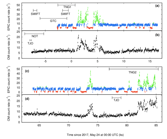
Figure 1: 0.3–10 keV EPIC light curve observed during XMM1 (panel a) XMM2 (panel c), binned every 10 s. Blue, red and green points indicate high, low and flaring mode intervals (see text for their definition). Panel (b) and (d) show the light curve observed by the Optical Monitor on board XMM-Newton and binned every 30 s. Horizontal bars indicate the intervals of simultaneous observations performed by other instruments.

Figure 2 shows the sum of the 3–79 keV light curves observed by two NuSTAR modules, binned at a time resolution of 100 s. We identified the transition using a light curve sampled in 10 s-long time bins, and setting the threshold between the low (red points) and the high (blue points) mode at a count rate of 0.15 s^-1, whereas the flaring (green points) took place at a rate higher than 0.9 s^-1. These threshold are similar to those determined by Tendulkar et al. (2014) and Coti Zelati et al. (2018); we set them by requiring that the the modes determined from the NuSTAR light curve would be the same as those observed by XMM-Newton during the 11.1 ks-long overlap occurring with XMM1. Due to the different photons statistics an exact correspondence could not be found; the threshold were conservatively set in order to avoid that the NuSTAR intervals deemed as flaring or low would be contaminated by high mode emission.

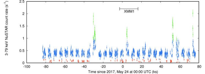
Figure 2: 3–79 keV light curve observed by NuSTAR binned at 100 s intervals. Red, blue and green points mark the low, high and flaring mode, respectively (see text for their definition). The horizontal bar indicates the interval covered by XMM1 observation.

3.1.2 Correlated optical/X-ray variability

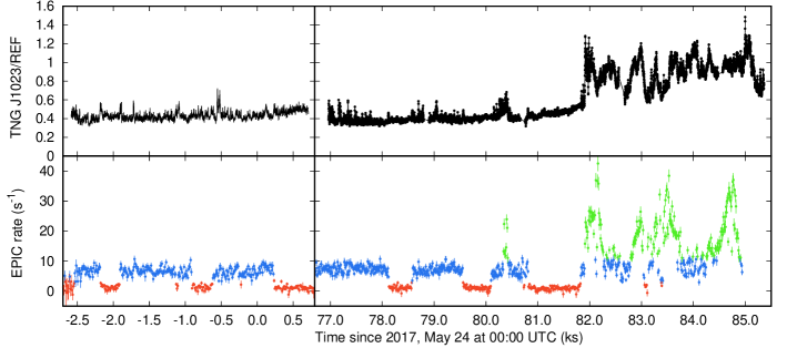
Figure 3: Differential TNG/SiFAP optical light curve of PSR J1023+0038 (top panel) and simultaneous XMM-Newton/EPIC coverage (bottom panel). Blue, red and green points indicate high, low and flaring mode intervals (see text for their definition).

The top panel of Figure 3 shows the differential TNG/SiFAP optical light curve defined as the ratio between the background subtracted count rate observed from PSR J1023+0038 and the reference star employed at the TNG, together with the simultaneous XMM-Newton/EPIC X-ray light curves in the respective bottom panels. Both light curves were binned every 10 s. Correlation between flares is evident, while there is no clear optical analogue of the high/low mode transitions observed in the X-ray band.

In order to explore the degree of correlation between the X-ray and the optical variability we considered the light curves observed by XMM-Newton/EPIC and TNG/SiFAP binned with a shorter timescale. The three intensity modes defined in Sec. 3.1.1 introduce a strong non-stationariety in the light curves. The cross-correlation function (CCF) requires stationarity, therefore we calculated a CCF for each mode. The intervals were selected based on the X-ray behavior, and were chosen carefully so as to exclude transitions. The CCFs were Scalculated using the HEASoft tool crosscor with a time resolution ranging from 1 to 2.5 s over 64 s intervals of the flaring, high and low modes; they are plotted in Fig. 4 with magenta, green and blue symbols, respectively. The inset of Fig. 4 shows the CCFs evaluated on a shorter time scale, ranging from 25 and 100 ms.

Our analysis shows that X-ray and optical emissions were clearly correlated in each of the three modes, with a somewhat similar behavior and degree of correlation. Namely, on timescales longer than a second (see Fig. 4), the optical variability showed a range of delays with respect to the X-ray variability, with a “reflection-like” CCF shape (O’Brien et al., 2002) which rises sharply in 2–3 s, peaks around zero, and decays slowly toward positive delays (i.e. optical lagging X-rays) reaching $\sim$10-20 seconds. On shorter timescales (see the inset of Fig. 4), the optical variability appeared instead to be correlated with the X-ray variability in the flaring mode with no evidence for delays. The CCF hints to a correlation also in the high mode, with no evidence for delays, while in the low mode the analysis is hampered by the lower statistics.

We note however that the shape of the CCFs depends strongly on the parameters chosen to calculate them, i.e. on the time resolution and on the length of the intervals over which the Fast-Fourier Transforms (FFT) were calculated. More importantly, when calculating the CCFs in the time domain (which by definition implies the use of “non strictly simultaneous” data intervals), we obtain different results. Finally, notwithstanding the rather low statistics, we have marginal evidence for the CCFs being variable in time. If confirmed, all this would imply that the variability is non-stationary even within a (X-ray) defined mode.

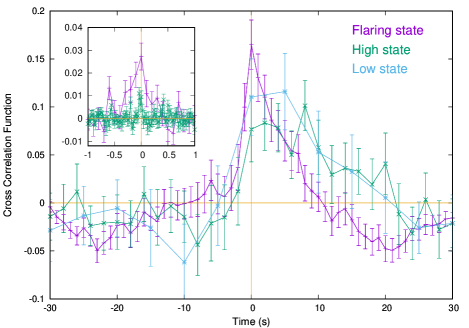
Figure 4: CCFs between the optical (TNG/SiFAP) and X-ray (XMM-Newton/EPIC) light curve observed during the flaring (magenta points), high (green points) and low (blue points) modes. A time resolution ranging between 1 and 2.5 s was used in the different modes, and 64 s-long intervals were averaged. The inset shows the CCF evaluated on a shorter time scale (ranging between 25 and 100 ms).

3.1.3 Correlated infrared/X-ray variability

The infrared light curve accumulated by CIRCE at GTC overlaps for 4.3 ks with the EPIC-pn exposure in XMM1. Fig. 5 shows the light curves observed in the infrared and X-ray bandwith with magenta and green symbols, respectively. Note that high particle background flaring affects the EPIC-pn light curve before MJD 57896.967, i.e. during the first 2.7 ks of the overlap with the CIRCE light curve, making it extremely noisy. The combination of this high background interval affecting the X-ray light curve and the short duration and low statistics of the infrared light curve prevented us to perform a quantitative study of the correlation between the X-ray and the infrared variability. However, a visual inspection of the two simultaneous curves provides clear evidence that they are correlated, with a slightly lower infrared flux during the X-ray low mode, when compared to the high mode. This is evident especially for the low mode occurring close to MJD 57896.976 (see Fig. 5).

Additionally, and perhaps more interestingly, there is also possible evidence for an increase of the infrared flux right after the transition from the low to the high X-ray mode. In other terms, the start of each X-ray high mode interval might be accompanied by a modest infrared flare. However this evidence is based on the presence of only three of such flares (i.e. those at about 0.94, 0.953 and 0.978 d since MJD 57896.0, the latter also seen in the TNG optical light curve, see the light curves in the left panel of Fig. 3 corresponding to -2 ks in the units used there) while in two additional occasions (0.962 and 0.971) no infrared flare seems to match the start of an X-ray high mode interval. Further and longer simultaneous observations are needed to confirm this result.

3.2 Timing Analysis

3.2.1 May 2017 campaign. The X-ray pulse

In order to perform a search for pulsations in the X-ray datasets we first corrected for the shifts of the photon arrival time caused by the orbital motion of the pulsar in the binary system. J16 showed that the epoch of passage of the pulsar at the ascending node of the orbit $T^{*}$ derived from the X-ray pulsations of PSR J1023+0038 shifts by up to tens of seconds with respect to any plausible solution based on a constant orbital period derivative. We then had to determine an orbital solution valid across the time span by the observations discussed here. We corrected the two XMM-Newton/EPIC-pn time series using the semi-major axis ($a\sin{i}/c=0.343356$  lt-s) and orbital period ($P_{orb}=17115.5216592$ s) of the J16 timing solution, and a grid of values of $T^{*}$ spaced by 0.125 s around the expected value. We carried out an epoch folding search on each of the time series by sampling each period with 16 phase bins, and estimated the best epoch of passage at the ascending node ($T^{*}=$57896.82926(1) MJD) by fitting with a Gaussian the values of the maximum pulse profile variance found in each of the periodograms we obtained. Figure 6 shows the difference $\Delta T^{*}$ between the epoch predicted by the radio timing solution of Archibald et al. (2013, see also Table 2 in J16) and the values measured from X-ray pulsations as a function of the number of orbital cycles performed since $T^{*}_{ref}=54905.97140075$ MJD. We took from Table 1 of J16 the values of $\Delta T^{*}$ measured before $\approx 13200$ cycles had elapsed since $T^{*}_{ref}$ (red points in Fig. 6), and added the last two measurements based on the analysis presented here ( blue points in Fig. 6; see below and Sec. 3.2.3). The epoch we measured of passage of the pulsar at the ascending node in May 2017 anticipated by $\Delta T_{asc}=$26.8(8) s the epoch predicted by the radio timing solution, confirming the $\sim 20$–$30$ s shift that occurred after the June 2013 state change already reported in J16, as well as the inability to describe with a polynomial of low order (or a sinusoidal variation, see the dashed line in Figure 6) the evolution of $T_{asc}$ over the years.

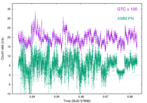
Figure 5: Light curves observed simultaneously by CIRCE/GTC in the Ks infrared band (magenta points, the observed rates were scaled by a factor 100) and by the XMM-Newton/EPIC in the 0.3–10 keV band (green points). A time resolution of 5.88 s was used.

In previous studies (Archibald et al. 2015, J16), X-ray pulsations were observed only during the high mode with an RMS amplitude of $\simeq 8\%$ and no detection was obtained during the low and flaring mode, with an upper limit of 2.4 and 1.4%, respectively. We performed a pulsation search on the mode-resolved EPIC-pn time series and obtained compatible results. Blue points in Fig. 7 show the epoch folding search periodograms obtained by folding with $n=16$ phase bins the high mode intervals observed during XMM1 (top panel) and XMM2 (bottom panel). We modeled the folded pulse profiles using two sinusoidal harmonics:

$$F(\phi)=\sqrt{2}(\bar{F}+\bar{B})\sum_{i=1}^{2}r_{i}\sin[2\pi i(\phi-\phi_{i})],$$ (1)

where $\bar{F}$ and $\bar{B}$ are the average source and background count rate, respectively, and $r_{i}$ and $\phi_{i}$ ($i=1,2$) are the RMS amplitude and phase of the two harmonics employed to model the pulse profile. We estimated the average period during the two observations by modeling the phases of the first and second harmonics of the pulse profile computed over 1.2 ks-long intervals using the phase residual formula (see, e.g., eq. 1 of Papitto et al., 2011), in which we let only the period of the pulsations and the epoch of passage of the pulsar at the ascending node free to vary. The second harmonic turned out to have a larger amplitude and provided the most accurate measurements, $P_{X}=1.6879874456(5)$ ms, compatible with the period expected according to the J16 solution, $P_{ref}=1.687987446019(3)$ ms, and $T^{*}=57896.829262(1)$ MJD. Blue points in Fig. 8 show the pulse profiles obtained by folding at $P_{ref}$ the high mode intervals of the two EPIC-pn observations. Table 2 lists the background-subtracted RMS amplitudes $r_{i}$ and phases $\phi_{i}$ ($i=1,2$) of the pulse profile, the total RMS amplitude $R=(\sum_{i}(r_{i}^{2}))^{1/2}$, the 0.3–10 keV flux $F_{abs}$ not corrected for interstellar absorption and evaluated by modeling the observed spectrum with an absorbed power law fixing the equivalent hydrogen column density to the value measured by Coti Zelati et al. (2014, $N_{H}=5\times 10^{20}$ cm^-2), the isotropic unabsorbed luminosity $L$ evaluated for a distance of 1.37 kpc (Deller et al., 2012) and the pulsed luminosity $L_{pulsed}=R\times L$. Upper limits on the pulse amplitude are computed at the 95% confidence level. We also measured the high mode RMS amplitude in four energy bands, and used these values to evaluate the pulsed flux. Cyan and blue points in Fig. 13 show the total and the pulsed flux in the high mode, respectively, expressed in $\nu F_{\nu}$ units; a dashed line indicates a $\nu F_{\nu}^{pulse}\sim\nu^{0.3}$ dependence, similar to that observed for the total flux.

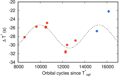
Figure 6: Difference between the epoch of passage of the pulsar at the ascending node of its orbit measured from X-ray pulsations and those expected according to the radio pulsar timing solution measured by Archibald et al. 2013 and J16 as a function of the number of orbital cycles elapsed since $T^{*}_{ref}=54905.97140075$. Red symbols refer to epochs measured by J16, blue symbols to measures from this work. Uncertainties on each measure range from 0.05 to 0.3 s. The dashed line shows a sinusoid with period equal to $\approx 5300$ orbital cycles, unable to explain the long-term trend.

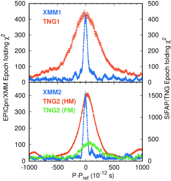
Figure 7: Epoch folding search periodograms of the XMM-Newton/EPIC-pn (blue points, left scale) and TNG/SiFAP (red points, right scale) time series in the high mode (HM), and TNG/SiFAP (green points, left scale) in the flaring mode (FM), observed during 2017, May 23 (top panel) and May 24 (bottom panel). Note that the scale used for the periodogram of TNG2 observation is reduced.

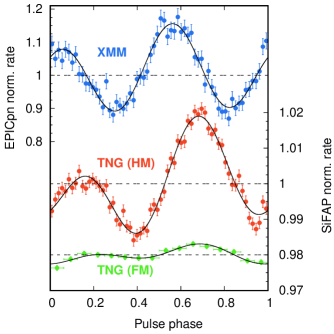
Figure 8: Pulse profiles obtained by folding the high mode intervals in the XMM-Newton/EPIC-pn data (blue points, left y-axis scale), the high mode intervals in the TNG/SiFAP data (red points, right y-axis scale) and the flaring mode intervals in TNG/SiFAP data (green points, right y-axis scale, shifted arbitrarily), around $P_{ref}$, with respect to the reference epoch MJD $57896.0$.

Table 2: Properties of the X-ray and optical pulses

Instrument	Band	$r_{1}$ ($\%$)	$r_{2}$ ($\%$)	$\phi_{1}$	$\phi_{2}$	R ($\%$)	$F_{abs}$	$L$	$L_{pulsed}$
High mode
XMM-Newton/EPIC-pn	0.3–10 keV	$2.9(3)$	$8.0(3)$	$0.33(2)$	$0.434(3)$	$8.5(4)$	$13.3(1)$	30.5(2)	2.6(1)
NuSTAR	3–79 keV	$<1.6$	$8.4\pm 1.3$	-	-	$8.4\pm 1.3$	$22(1)$	49(2)	4.1(7)
TNG/SiFAP	320–900 nm	$0.63(2)$	$0.74(2)$	$0.473(7)$	$0.548(3)$	$0.97(2)$	$4.2(2)$	11.5(4)	0.111(5)
Low mode
XMM-Newton/EPIC-pn	0.3–10 keV	-	-	-	-	$<3.0$	$2.6(1)$	6.1(2)	$<0.18$
NuSTAR	3–79 keV	-	-	-	-	$<14.0$	$2.4(4)$	5.4(9)	$<0.75$
TNG/SiFAP	320–900 nm	$<0.03$	$<0.02$	-	-	$<0.034$	$4.4(2)$	12.1(4)	$<0.004$
Flaring mode
XMM-Newton/EPIC-pn	0.3–10 keV	-	-	-	-	$<1.3$	$37.6(5)$	87.1(9)	$<1.1$
NuSTAR	3–79 keV	-	-	-	-	$<6.9$	$61(8)$	$137\pm 18$	$<9.5$
TNG/SiFAP	320–900 nm	$0.12(2)$	$0.11(2)$	$0.37(2)$	$0.58(1)$	$0.16(2)$	$8.5(4)$	23(1)	0.037(5)

Note. — Pulse profiles were obtained folding the respective time series in 64 phase bins (reduced to 16 in case of a low significance detection or to derive upper limits) around $P_{ref}=1.687987446019$ ms and setting $T_{ref}=57896.0$ MJD as the reference epoch. $r_{i}$ and $\phi_{i}$ are the background-subtracted RMS amplitude and phase (in cycles), respectively, of the first ($i=1$) and second ($i=2$) harmonic used to model the pulse profiles, $R=(r_{1}^{2}+r_{2}^{2})^{1/2}$ is the total RMS amplitude, $F_{abs}$ is the flux in units of $10^{-12}$ erg cm^-2 s^-1 not corrected for interstellar absorption and observed in the bands listed in the second column, $L$ is the isotropic luminosity in units of $10^{32}$ erg s^-1 corrected for interstellar absorption and evaluated for a distance of 1.37 kpc (Deller et al., 2012), and $L_{pulsed}=R\times L$ is the pulsed luminosity evaluated using the same parameters.

We searched the 3–80 keV NuSTAR time series for a coherent signal, computing power density spectra over 3.3 ks intervals. The average of the 28 power spectra so obtained shows an excess centered at 1184.8430(1) Hz interpreted as the second harmonic of the signal at the spin period of PSR J1023+0038. The peak in the power density spectrum is broad with a width compatible with the spurious derivative of $10^{-10}$ Hz/s introduced by the NuSTAR clock drift (Madsen et al., 2015), and corresponds to an rms pulse amplitude of $(6.8\pm 1.3)$%. To determine a more precise value of the pulsation period we performed an epoch-folding search of the whole NuSTAR data around the corresponding fundamental frequency obtained from the analysis of the power density spectrum with steps of $3\times 10^{-14}$ s, for a total of 10001 steps. The pulse profile with the largest signal-to-noise ratio corresponds to the period $P_{NuSTAR}=1.687987299(1)$ ms that differs by $1.5\times 10^{-10}$ s from $P_{ref}$. We also searched for a signal in the time series restricted to the three modes. The signal was detected in the high mode with an overall rms amplitude of $(8.4\pm 1.3)\%$, roughly constant up to 45 keV. The pulsed flux spectral distribution (see green points in Fig. 13, where the total flux is also plotted with light green points) observed by NuSTAR in the high mode is compatible with the power law relation $\nu F_{\nu}\sim\nu^{0.3}$ indicated by XMM-Newton data. On the other hand, upper limits of $14.0\%$ and $6.9\%$ (95% confidence level) were set on the pulse amplitude during the low and the flaring mode, respectively.

3.2.2 May 2017 campaign. The optical pulse

We used the low, high and flaring mode time intervals determined using the EPIC light curves to select the corresponding intervals during the TNG observations. Table 2 lists the properties of the optical pulse during the three modes. We detected optical pulses at a high confidence level during the high mode (red points in Fig. 7 show the periodogram) with an average, background-subtracted RMS amplitude of $(0.68\pm 0.02)\%$. Note that since the background is probably overestimated during TNG1 (see Sec. 2.6), the actual intrinsic pulse amplitude was likely slightly larger. The top panel of Fig. 9 shows the evolution of the RMS amplitude over high mode time intervals of length ranging from $\sim 200$ to $450$ s; it attains values as high as $R_{max}=(1.4\pm 0.1)\%$, and is variable although with no clear correlation with the orbital phase. Towards the end of TNG2 the pulse amplitude decreased down to a level comparable to that observed during flares ($<0.2\%$, see below), suggesting that the entire interval from $\sim 82$ ks since May 24 00:00 to the end of TNG2 (see right panels of Fig. 3) was in the flaring mode. By considering only the high mode intervals before the onset of such a long flaring event, the average pulse fraction observed in the high mode increased to $R_{HS}=(0.97\pm 0.02)\%$. Similar to the X-ray band, the optical pulse was not detected during the low mode down to an upper limit of $0.02\%$ (95% confidence level), i.e roughly 30 times smaller than the amplitude observed during the high mode. The flaring mode took place only during TNG2 and the optical pulse was detected at a significance of 8.3$\sigma$ and with amplitude $R_{2,flare}=(0.16\pm 0.02)\%$, i.e. more than five times smaller than during the high mode. Considering that the net count rate observed by SiFAP/TNG during flares is about twice that in the high mode, the amplitude decrease is larger than what would be expected if the flares were a simple addition of unpulsed flux to the high mode level. We checked that optical pulses were detected at a significance larger than 4.5$\sigma$ even when flares were identified by using a higher threshold in the EPIC X-ray light curve, $20$ s^-1, rather than $11$ s^-1, the value used by Bogdanov et al. (2015) and throughout this paper.

We performed pulse phase timing on the optical pulse profiles computed over intervals of length spanning between 200 and 500 s in the high mode. We measured an optical period $P_{opt}=1.687987445(1)$ ms, a value compatible with $P_{ref}$ and $P_{X}$, and the epoch of passage at the ascending node $T^{*}_{opt}=57896.829267(6)$ MJD, compatible with the X-ray estimate within $\delta T^{*}\sim 0.5$ s. This estimate can be used to constrain the position of the region emitting the optical pulses within $a_{1}\delta T^{*}/P_{orb}\simeq 3(\sin(i))^{-1}$ km in azimuthal distance along the orbit from the region emitting the X-ray pulses, where $a_{1}$ is the semi-major axis of the pulsar orbit and $i$ is the system inclination.

Red and green points in Fig. 8 show the normalized and background-subtracted optical pulse profiles observed in the high and flaring mode, respectively. The optical pulse is described by two harmonics with an amplitude ratio $r_{2}/r_{1}\simeq 1$, smaller than that of the X-ray pulse ($\simeq 3$; blue points in Fig. 8)). The phase of both harmonic components of the optical pulse profile lag the corresponding components of the X-ray profile; the lags of the first and second harmonic are $\delta\phi_{1}=0.14\pm 0.01$ and $\delta\phi_{2}=0.112\pm 0.004$, respectively. The phase difference observed during periods of strictly simultaneous observations is compatible with these estimates, indicating that the phase lag is not due to variability of the X-ray pulse profile in intervals not overlapping with the optical observations. The bottom panel of Fig. 9 shows the evolution of the phase of the two harmonic components of the optical (blue dots and cyan hollow squares for the first and second harmonic, respectively) and X-ray (green dots and red hollow squares) pulse profiles over the interval of simultaneous coverage; a phase shift of $\approx 0.1$ is always observed, with a somewhat larger timing noise shown by the optical pulse.

We measured the average optical flux $F_{abs}$ in different modes by scaling the observed background-subtracted count rate by the conversion factor determined in Sec. A.1. We estimated the pulsed luminosity by scaling these flux values for the ratio between the de-reddened and the absorbed flux in the 320–900 nm energy band ($k_{der}=1.217$) and multiplying for the total RMS amplitude we obtained the pulsed luminosity shown in the rightmost column of Table 2. The values obtained in this way are listed in of Table 2. A red point in Fig. 13 shows the average de-reddened pulsed flux observed during the high mode ($5.2(4)\times 10^{-14}$ erg cm^-2 s^-1) in $\nu F_{\nu}$ units, computed assuming a constant value over the 320–900 nm band.

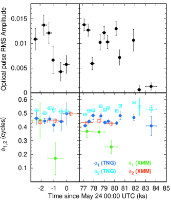
Figure 9: Top panel: the RMS amplitude of the optical pulse along the May 23 (left) and May 24 (right) observing runs during the high mode. Lower Panel: the phases of the optical pulse as measured in the May 23 (left) and May 24 (right) TNG runs (blue dots and sky blue empty squares were used for the first and second harmonic, respectively), and the phases of the X-ray pulse as measured in the two XMM-Newton runs (green dots and red empty squares were used for the first and second harmonic,respectively).

3.2.3 December 2017 campaign. The optical pulse

We preliminary measured the epoch of passage of the pulsar at the ascending node correcting the time of arrival of TNG3 with the semi-major axis and orbital period of the J16 timing solution, and varying a grid of values of $T_{asc}$ spaced by 0.2 s around the expected value. We corrected the event arrival times of TNG3 with the preliminary value of $T_{asc}$, and folded the resulting time series around $P_{ref}$. We measured the pulse phase of the first and second harmonic of the pulse and determined $P_{TNG3}=$1.687987456(12) ms (compatible with the value expected according to the J16 solution, 1.687987446177(4) ms), and $T^{*}_{TNG3}=58107.009511(4)$ MJD. Blue, green and red points in Fig. 10 mark the RMS amplitude (top panel) and the phases (dots show those computed on the first harmonic, hollow squares indicate phases of the second harmonic) of the pulse profiles observed during the exposures performed with B, V and R filters, respectively, and measured using the J16 ephemerides and the same reference epoch used fold May 2017 data. The phase difference of $\simeq 0.2$ cycles shown by the phases computed over the first and second harmonic with respect to the values observed during May 2017 (see Table 2 and bottom panel of Fig. 9) is compatible with the $0.1$ cycles phase uncertainty obtained propagating the errors on the ephemerides given by Jaodand et al. 2016 to the epoch of TNG3. A comparison between the pulse phase measured at different epochs is further hampered by the noise affecting the measured epoch of passage at the ascending node (see Fig. 6). Note that the absence of simultaneous X-ray observations prevented us from identifying transitions between the high and low modes (flares are not evident in the light curves); since pulses are absent in the low mode, the amplitudes plotted in Fig. 10 are underestimated with respect to the values measured in the high mode alone. Note that the source spends on average $\sim 70-80\%$ of the time in the high mode (J16).

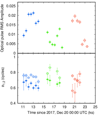
Figure 10: The top panel shows the RMS amplitude of the optical pulse profiles observed during TNG3-B (blue points), TNG3-V (green points) and TNG3-R (red points) by folding the time series around $P_{ref}$ and choosing MJD $58107.0$ as the reference epoch. The bottom panel shows the phase computed over the first (filled circles) and the second harmonic (hollow squares).

3.2.4 December 2017 campaign. The X-ray pulse

We analyzed three NICER observations performed in December 2017. The bottom panel of Fig. 11 shows a sample light curve observed during the first observation, where the high, low and flaring modes can be easily recognized.

Adopting the orbital ephemerides from the timing analysis of the TNG3 data, we corrected the NICER photon arrival times and searched for coherent pulsations by computing power density spectra over 2 ks-long intervals. A statistically significant excess at $\nu=1184.8426(5)$ Hz is observed in the average power density spectrum, consistent with the second harmonic of the spin frequency of the source. We applied epoch-folding search techniques to the available NICER observations around the spin period extrapolated from the coherent signal detected with the Fourier analysis. We obtained the best profile for the spin period $P_{NICER}=$1.6879874457(4) ms, compatible with the value expected according to the J16 solution. The average profile is characterized by an RMS amplitude $R=(5.3\pm 0.7)\%$. Extrapolating the count rate threshold adopted for XMM-Newton/EPIC-pn data, we investigated coherent signals in the time series restricted to the three modes. Similarly to the XMM-Newton/EPIC-pn case, we did not detect any signal in the low and flaring modes. On the other hand, we detected pulsation in the high mode with amplitude of $(5.6\pm 0.9)\%$ , with a second harmonic roughly three times times stronger than the fundamental (see top panel of Fig. 11).

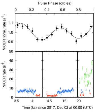
Figure 11: Pulse profile obtained by folding the high mode intervals in the NICER data with respect to the reference epoch MJD 57896.0, using J16 ephemerides and the epoch of passage at the ascending node determined from December 2017 optical data (see Sec. 3.2.3), $T^{*}_{TNG3}=58107.009511(4)$ MJD (top panel). Light curve observed by NICER during observation 1034060101 (see Tab. 1, bottom panel).

3.3 The optical spectrum

Figure 12 shows the optical spectrum observed by ALFOSC/NOT, calibrated in flux using the simultaneous measurement of the magnitude by the TJO (see Sec. 2.10). Broad, in a few cases double peaked emission lines of H$\alpha$ 656.3, H$\beta$ 486.1, HeI 587.6, HeI 667.8, HeI 501.5, HeII 468.6, HeI 447.1 nm are most prominent. Telluric contamination produced the absorption line at $\simeq 687$ nm. These features have double-peaked profiles which are signature of an accretion disk viewed at moderate inclination. As the continuum is blue and smooth (see Fig. 2 Wang et al., 2009), we created a template spectral shape, $f_{1023,NOT}(\lambda)$ by extrapolating the continuum observed at NOT to the 320–900 nm band, giving a flux of $F_{J1023,NOT}\simeq 3.8\times 10^{-12}$ erg cm^-2 s^-1 over this band.

Figure 12: Optical (440–695 nm) spectrum of PSR J1023+0038 taken with ALFOSC at the NOT. The most prominent emission lines are marked with a vertical segment. The spectrum was normalized to match the flux density observed simultaneously by TJO in the V-band ($V=16.85\pm 0.02$ mag, corresponding to $(6.9\pm 0.1)\times 10^{-15}$ erg cm^-2 s^-1 nm^-1 at 550 nm. During the same interval of NOT observations, the OM on-board XMM-Newton observed a count-rate of $6.1(1)$ s^-1, which translates into a flux density of $7.9\times 10^{-15}$ erg cm^-2 s^-1 nm^-1 at 450 nm.

4 Discussion

This paper presented the first high time resolution optical/X-ray/IR/UV observational campaign of PSR J1023+0038 in the disk state. Similar to other transitional millisecond pulsars in such a state, the X-ray light curve of PSR J1023+0038 shows three intensity modes (dubbed low, high and flaring), and coherent X-ray pulsations were detected only in the high mode; they have an rms amplitude of $\simeq 8\%$ and are detected up to 45 keV, as first shown in this study based on NuSTAR observations.

Our simultaneous optical/X-ray observations revealed that also optical pulses are observed in the high mode. Optical pulses have an average rms amplitude of $R_{HS}=(0.97\pm 0.02)\%$, corresponding to a pulsed luminosity of $\bar{L}_{HS}=1.11(5)\times 10^{31}$ erg s^-1 (see Table 2). The spin period and the epoch of passage at the ascending node measured from the optical pulses are consistent with the values measured in the X-ray band within $(0.6\pm 1.2)\times 10^{-12}$ s and $(0.4\pm 0.5)$ s, respectively. The latter estimate indicates an azimuthal distance of a few km at most between the region emitting the optical and X-ray pulses, indicating that the optical and X-ray pulses are produced in the same region. Assuming a constant flux over the 320–900 nm band, $F_{\nu}\sim$ count’s, we estimated the average pulsed flux density of $\bar{S}_{\nu}=10.7(6)\,{\mu}$Jy. This value is compatible with the low-frequency extrapolation of the $F_{\nu}\propto\nu^{-0.7}$ trend that holds for the pulsed flux density in the X-ray band (see Fig. 13), suggesting that such a component could describe the pulsed spectral energy distribution over at least four decades in energy. The optical pulse amplitude was highly variable between 0.5 and 1.5% over 500 s-long intervals, corresponding to a maximum pulsed luminosity of $L_{HS}^{max}\simeq 1.6(1)\times 10^{31}$ erg s^-1.

Similar to X-ray pulses, optical pulses were not detected in the low mode, with an upper limit of $R_{LS}<0.034\%$ (95% confidence level). This corresponds to a pulsed luminosity of $4\times 10^{29}$ erg s^-1, i.e. more than 25 times smaller than the value observed in the high mode.

The simultaneous detection of pulses in the optical and X-ray bands breaks down during flares. Optical pulses were detected with an rms amplitude of $R_{FL}=(0.16\pm 0.02)\%$, corresponding to an average pulsed luminosity of $0.37(5)\times 10^{31}$ erg s^-1, i.e. almost one third than the average value observed in the high mode. X-ray pulsations remained undetected down to an amplitude of $1.3\%$, corresponding to a pulsed flux $2.3$ times lower than in the high mode. If the X-ray pulsed fraction decreases during flares with respect to the high mode by the same amount seen in the optical, we expect them at an amplitude of $\sim 1\%$, i.e. slightly lower than the upper limit we derived. We conclude that the non-detection of X-ray pulses during flares may result from limited photon statistics.

Both the optical and X-ray pulses were described by the sum of two harmonic components, yielding two intensity peaks every NS rotation. The ratio of the second to the first harmonic amplitude of the optical pulse $r_{2}/r_{1}$ was close to unity, lower than the value observed in the X-ray band ($\simeq 3$). The first and the second harmonic of the optical pulse lagged the X-ray pulse by $\delta\tau_{1}=236\pm 17\mu$s and $\delta\tau_{2}=189\pm 7$ $\mu$s, respectively. Lags of the same order were observed over intervals of few hundreds seconds, in both simultaneous optical/X-ray observations analyzed here. The absolute timing accuracy of XMM-Newton is 48$\,\mu$s (Martin-Carrillo et al., 2012). On the other hand, we estimated the SiFAP absolute time accuracy as better than $\sim 60\,\mu$s, by relying on a hour-long observation of the Crab pulsar performed at the Cassini Telescope at Loiano Observatory (see A1). The resulting total systematic error affecting the phase lag between the optical and X-ray pulse is $<77\,\mu$s.

Optical pulses were seen at an amplitude varying between 0.5 and 2% in the Johnson B, V and R filters. In the absence of simultaneous observations of a reference star and the X-ray counterpart we could not measure accurately the optical spectral energy distribution.

The main result presented in this paper is that optical and X-ray pulses closely trace the repeated transitions between the X-ray high mode, in which they are both observed and whose pulsed flux is compatible with a single power law relation $F_{\nu}\propto\nu^{-0.7}$, and the low mode, in which they are not detected. This strongly indicates that optical and X-ray pulses are related to the same phenomenon, something also suggested by the similar pulse shape and small phase offset. In the following we discuss the implication of these findings for the different scenarios proposed to explain the enigmatic nature of the disk state shown by PSR J1023+0038 and other transitional millisecond pulsars.

4.1 Accretion onto the NS surface and propelling of matter

Coherent X-ray pulsations seen in the high mode of PSR J1023+0038 were first interpreted as due to magnetically channeled accretion onto the NS hot spots (Archibald et al., 2015). This interpretation was justified by the ten-fold increase in the X-ray pulsed and total flux that occurred after an accretion disk formed in the system in June 2013, as well as the similarity of the pulsed fraction, shape and spectrum of the X-ray pulses observed from PSR J1023+0038 to those shown by accreting millisecond pulsars. Based on a similar reasoning Papitto et al. (2015) interpreted in terms of accretion power also the X-ray pulsations shown by the transitional millisecond pulsar XSS J12270-4859 in the disk state. However, as both authors noted, interpreting such X-ray pulses as due to channeled accretion challenged the usual accretion/propeller picture for fast rotating NS. To show this, we assume that the disk is truncated at a radius equal to $\xi$ times the Alfven radius,

$$r_{m}=57.6~{}\xi_{0.5}~{}\mu_{26}^{4/7}\,\dot{m}_{14}^{-2/7}~{}m_{1.4}^{-1/7}~{}km$$ (2)

where $\xi_{0.5}=(\xi/0.5)$, $\dot{m}_{14}$ is the mass accretion rate in units of $10^{14}$ g s^-1 and $\mu_{26}$ is the magnetic dipole moment in units of $10^{26}$ G cm^-3 ($\mu_{26}=0.79\,(1+\sin^{2}\alpha)^{-1}$ for PSR J1023+0038, with $\alpha$ angle between the magnetic and the spin axes, evaluated using the spin-down rate during the radio-pulsar phase measured by J16 into the relation given by Spitkovsky 2006). The observed X-ray luminosity ($\simeq 8.5\times 10^{33}$ erg s^-1 in the 0.3–80 keV band, Coti Zelati et al. 2018) indicates a mass accretion rate of $\dot{m}_{14}=0.46~{}m_{1.4}^{-1}$, where $m_{1.4}$ is the NS mass in units of 1.4 M_⊙, and according to Eq. 2, a disk radius of $r_{m}\simeq 72\,\xi_{0.5}$ km. Taking $\xi_{0.5}=1$, this value exceeds by three times the corotation radius of PSR J1023+0038 ($r_{c}$=23.8 $m_{1.4}^{1/3}$ km) and accretion onto the NS surface should be inhibited by the quick rotation of magnetic field lines at the magnetospheric boundary.

Papitto & Torres (2015) proposed that the magnetosphere would be squeezed to $\sim r_{c}$ if the actual accretion rate in the disk were larger ($\dot{m}_{14}=5-17$) than the value indicated by the X-ray luminosity. In such a case 99% of the mass should be ejected from the inner rim of the disk by the propelling magnetosphere in order to match the relatively low X-ray flux. Roughly half of the X-ray emission and the whole gamma-ray output would be due to synchrotron self-Compton emission by electrons accelerated in the shock formed at the disk-magnetosphere boundary (see also Papitto et al. 2014). Alternatively, the disk could have fallen in a low $\dot{M}$ trapped state (D’Angelo & Spruit, 2012) with its inner rim that stays close to the corotation radius regardless of how low the mass accretion rate could get. In the case of PSR J1023+0038, such a model would imply that the observed X-ray luminosity traces the actual mass accretion rate and a strong outflow would not be launched.

Assuming that X-ray pulses are due to accretion of matter onto the magnetic poles, the optical pulses of PSR J1023+0038 could be explained by cyclotron emission by electrons inflowing in magnetized accretion columns, similar to the case of accreting magnetic white dwarfs (Masters et al., 1977; Lamb & Masters, 1979). Indeed, the fundamental cyclotron energy for electrons inflowing in accretion columns permeated by a magnetic field of the order of that estimated for PSR J1023+0038 (Archibald et al., 2013, J16) is $E_{cyc}=1.2$ eV. Assuming that $\beta$ is the angle between the magnetic axis and the disk plane, matter inflowing from a disk truncated at the corotation radius $r_{C}$ forms hot-spots on the neutron star surface of size:

$$A_{spot}\simeq\pi\frac{r_{*}^{3}}{r_{c}}\sin^{2}{\beta}=1.3\times 10^{12}~{}\sin^{2}{\beta}~{}cm^{2},$$ (3)

i.e. $\sim 10\%$ of the NS surface, in agreement with the results of the simulations performed by Romanova et al. (2004). The corresponding typical accretion column transverse length-scale is then $\ell\simeq 5$ km, and the electron density in the accretion columns for a fully ionized plasma is:

$$n_{e}=\frac{\mu_{e}}{m_{H}}\rho=\frac{\mu_{e}}{m_{H}}\frac{\dot{M}}{\pi\ell^{2}v_{ff}}=0.5\times 10^{16}\,\dot{m}_{14}\,\ell_{5}\,m_{1.4}^{-1/2}\,cm^{-3}$$ (4)

where $\mu_{e}=1.18$ is the mean molecular weight per electron, $m_{H}$ is the proton mass, $v_{ff}=\sqrt{2GM/r_{*}}$ is the free-fall velocity close to the NS surface and $\ell_{5}\equiv\ell/5~{}\mbox{km}$. The resulting optical depth to cyclotron absorption of accretion columns filled by plasma of such density and permeated by a $B\sim 10^{8}$ G magnetic field is as large as $\approx 10^{6}$ in the transverse direction (Trubnikov, 1958). This ensures that the emission of the first few cyclotron harmonics is self-aborbed (up to roughly ten), and that the resulting spectrum is described by the Rayleigh-Jeans section of a black-body spectrum with temperature equal to the electron temperature, $T_{e}$.

However, in Ambrosino et al. (2017) we estimated the maximum cyclotron luminosity expected in the 320-900 nm band as:

$$L_{cyc} = A_{spot}\int_{\nu_{l}}^{\nu_{h}}(2\pi kT_{e}\nu^{2}/c^{2})d\nu=$$ (5)

$$= 2.9\times 10^{29}\left(\frac{A_{spot}}{10^{12}cm^{2}}\right)\left(\frac{kT_{e}}{100keV}\right)\,erg\,s^{-1},$$

where $\nu_{l}=3.33\times 10^{14}$ Hz and $\nu_{h}=9.37\times 10^{14}$ H¡ are the boundaries of the band observed by SiFAP. This value is $\approx 40$ times lower than the observed average optical pulsed luminosity. This discrepancy holds even when taking for $kT_{e}$ a value of $\sim 100$ keV, of the order of that observed from accreting millisecond pulsars (Patruno & Watts, 2012, and references therein), and likely an overestimate of the temperature attained by electrons in the accretion column of a pulsar with an accretion luminosity of $<10^{34}$ erg s^-1. In fact, such a high electron temperature can be reached if the pressure exerted by the radiation emitted from the hot-spots balances the gravitational inflow of plasma in the accretion columns, and forms a shock standing off the NS surface, where the kinetic energy of the flow is converted into thermal motion of the charges. The critical luminosity to form such a shock is $L_{crit}\approx 10^{36}\,\ell_{5}$ erg s^-1 (Basko & Sunyaev, 1976), more than a hundred times larger than the value observed from PSR J1023+0038. Below such a value the ions of the in-falling plasma are best slowed down by Coulomb collisions with atmospheric electrons (Frank et al., 2002, see, e.g.,), and a temperature of the order of the effective black-body temperature is attained, $kT_{e}\simeq 1.9(L/L_{crit})^{1/4}$ keV. We deduce that magnetic accretion at a rate $L\sim 10^{-3}L_{crit}$ is hardly capable to produce electrons hot enough to yield a sizable cyclotron emission in the optical band (e.g. $L_{cyc}\simeq 10^{27}$ erg s^-1 for $kT_{e}\simeq 0.3$ keV).

According to Eq. 5, the maximum observed pulsed optical luminosity $L_{HS}^{max}\simeq 1.6(1)\times 10^{31}$ erg s^-1 corresponds to an unrealistically large brightness temperature of $kT_{b}=(175\pm 10)~{}(r_{em}/\mbox{km})^{-2}$ MeV, where $r_{em}$ is the radius of the emission region. Even considering $r_{em}\sim 100$ km (i.e. approximately the size of the light cylinder), the X-ray luminosity that would be produced by such a thermal component ($\sim 10^{44}$ erg s^-1) would be huge. We can then safely rule out emission from hot-spots on the NS surface heated by the accretion flow as the origin of optical pulses. A similar reasoning rules out reprocessing of the X-ray emission by the inner regions of the disk, which would necessarily produce an even cooler and fainter thermal spectrum,

4.2 Rotation-powered pulsar

An alternative possibility is that the optical pulsations of PSR J1023+0038 originate in the activity of a rotation-powered pulsar. So far, optical pulsations have been detected from five isolated high-magnetic field young pulsars (Mignani, 2011, and references therein). Models envisage that synchrotron emission of secondary electron/positron pairs accelerated in magnetospheric gaps, re-connection events and/or the equatorial current sheet (see, e.g., Venter et al., 2018, for a recent review) give rise to non-thermal pulsed emission at optical and X-ray energies (Pacini & Salvati, 1983), whereas curvature radiation accounts for the gamma-ray emission (Romani, 1996). Recently, the need of using a common description of these processes, dubbed as synchro-curvature, has become evident since both effects are relevant along the particles trajectories in the magnetosphere (Viganò et al., 2015). These mechanisms are unlikely to work if the magnetosphere is engulfed with plasma from the disk (density of $n_{e}\simeq 5\times 10^{15}$ cm^-3, see Eq. 4, i.e. $\approx 10^{6}$ times the Goldreich & Julian critical density, Goldreich & Julian 1969) as gaps in the outer magnetosphere would be readily filled (Shvartsman, 1971). Even if electron acceleration up to a Lorentz factor $\gamma_{3}\equiv\gamma/10^{3}=1$ were possible, charges would be stopped down by Coulomb collisions with ions and electrons of the plasma on a typical length-scale of $\approx 5\times 10^{-5}\gamma_{3}^{-1}$ cm (see, e.g., Eq. 3.35 in Frank et al., 2002). This is much smaller than the length over which electrons radiate synchrotron X-ray and optical photons in a pulsar magnetosphere, $<10^{-5}r_{LC}\simeq 80$ cm for PSR J1023+0038 after particle injection (Torres, 2018). For this reason we assume that a rotation-powered pulsar is able to work only if the matter inflow is truncated outside the light cylinder, and no accretion onto the NS surface takes place. To meet this condition, the mass accretion rate should be lower than $\dot{m}_{14}<0.3\,\xi_{0.5}^{7/2}$ (see Eq. 2 for $r_{m}>r_{LC}$), and the inferred luminosity lower than $2.5\times 10^{32}$ erg s^-1. In this scenario most of the observed X-ray luminosity ($\simeq 8.5\times 10^{33}$ erg s^-1) would not be due to disk accretion.

However, assuming that the optical pulses of PSR J1023+0038 originate in the magnetosphere of a rotation-powered pulsar presents a number of issues. First, a very large efficiency is required to explain the conversion of up to ${L}_{HS}^{max}/\dot{E}\simeq 3.6\times 10^{-4}$ of the spin down power $\dot{E}=4.4\times 10^{34}$ erg s^-1 (Archibald et al., 2013) in 320–900 nm optical pulsed luminosity. Values lower by at least an order of magnitude are observed from other powerful rotation powered pulsars, including the Crab pulsar (Percival et al., 1993) and the isolated millisecond pulsar PSR J0337+1715 (Strader et al. 2016; see Fig. 3 of Ambrosino et al. 2017, which compares the optical efficiency in the B-band of various types of pulsars).

Secondly, the pulsed X-ray luminosity in the high mode was $\simeq 2.6\times 10^{32}$ erg s^-1 (Archibald et al., 2015, see also Table 2), i.e. $\sim 6\times 10^{-3}$ times the spin down power. The simultaneous detection of optical and X-ray pulses in the high mode and their disappearance in the low mode means that if the former has a magnetospheric origin, likely also the latter does. The fraction of the spin-down power converted in X-ray pulses of PSR J1023+0038 would be much larger than that of almost all rotation-powered pulsars ($<10^{-3}$, Possenti et al. 2002; Vink et al. 2011, see also Lee et al. 2018 for an updated analysis that suggests an average efficiency $\simeq 10^{-4}$). Considering that rotation-powered pulsars with sinusoidal pulse profiles generally show a pulsed fraction of $\sim 10\%$ (Zavlin, 2007), the discrepancy is likely even larger. More importantly, when a disk was absent and radio pulses were observed, Archibald et al. (2010) detected X-ray pulsations in the 0.25-2.5 keV band with an rms amplitude of $(11\pm 2)\%$. Even assuming that pulsations were present also in the 2.5–10 keV band and with the same amplitude (note that in that band Archibald et al. (2010) could only place a 20% upper limit on the pulse amplitude), the pulsed X-ray luminosity would have been $\sim 10^{31}$ erg s^-1, i.e. $2\times 10^{-4}$ times the spin-down power. The 25-fold increase of the pulsed flux that occurred when a disk formed in the system would be very difficult to explain assuming that the rotation-powered pulsar kept working as if it were in the radio pulsar state. One case of mode switching by an isolated rotation-powered pulsar is known (Hermsen et al., 2013; Mereghetti et al., 2016), but it appears contrived that the mode change of PSR J1023+0038 which occurred when a disk formed was not influenced by it.

The large optical and X-ray spin down conversion efficiency needed to produce a magnetospheric emission large enough to explain the observed pulsed flux could be indeed related to the presence of the disk. Soft disk photons could enhance the pair production in the magnetosphere yielding a brighter pulsed radiation than in the radio pulsar state in which the system roughly behaves as if it were isolated. However, a simultaneous fit of the gamma-ray and X-ray emission of PSR J1023+0038 with models developed for rotation-powered pulsars was troublesome. We considered the synchro-curvature model developed by Torres (2018). The model was shown to be able to describe well the X-ray and gamma-ray emission of rotation-powered pulsars in terms of a few order parameters (such as the accelerating electric field, a measure of how uniform the distribution of particles emitting towards us, the magnetic gradient along a field line and a normalization). Particularly, in all cases in which both energy bands displayed pulsed emission, the spectral model built out of only the gamma-ray data is close to the detected X-ray emission spectrum already, and further common analysis of both energy regimes makes for a perfect agreement (Torres, 2018; Li et al., 2018). This has proven not to be the case here: we attempted to model the gamma-ray/X-ray pulsed energy distribution observed from PSR J1023+0038 (see Fig. 13), but even assuming that the gamma-ray emission comes entirely from the magnetosphere (note that gamma-ray pulses have not been detected from PSR J1023+0038 in the disk state, so far), varying the relevant magnetospheric parameters over the wide range used in Torres (2018) gives an X-ray and optical pulsed output lower than observed by one and three orders of magnitude, respectively. Based on the different behavior found for PSR J1023+0038 when compared to all other pulsars studied from the synchro-curvature model we conclude that the magnetospheric activity of a rotation-powered pulsar that works as if it were isolated (and with most of the gamma-ray radiation pulsed) is unlikely the only source of the optical/X-ray pulses observed from PSR J1023+0038.

4.3 Pulsar wind

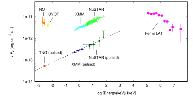
Figure 13: Total and pulsed spectral energy distribution of PSR J1023+0038 in the high mode, corrected for interstellar extinction. The NOT optical spectrum (see Sec. 3.3) is plotted with an orange line. The average pulsed TNG/SiFAP optical flux observed in May 2017 (see Sec. 3.2.2) is plotted with a red square. The flux observed by Swift/UVOT UVW1 is plotted with a yellow square. The total and pulsed X-ray flux observed by XMM-Newton (see Sec. 3.2.1) are plotted with light and dark blue points, respectively. The total and pulsed X-ray flux observed by NuSTAR (see Sec. 3.2.1) are plotted with light and dark green points, respectively. Magenta squares show the average Fermi-LAT spectrum measured by (Torres et al., 2017). The dashed line is a cut-off power law $\nu F_{\nu}\sim\nu^{0.3}$ normalized to match the optical and X-ray observed pulsed flux.

We suggest an alternative interpretation of the optical and X-ray pulses shown by PSR J1023+0038 in terms of synchrotron radiation emitted from the intrabinary termination shock of the pulsar wind with the accretion disk in-flow at a distance $kr_{LC}$, with $k=1$–2, i.e. just beyond the light cylinder (see Fig. 14 for a schematic diagram of the geometry we have assumed; see also Veledina et al. (2019) who have presented an interpretation based on similar assumptions). For an isotropic pulsar wind, the post-shock magnetic field is (Arons & Tavani, 1993):

$$B_{s}=3\left(\frac{\sigma}{1+\sigma}\right)^{1/2}\left(\frac{\dot{E}}{cf_{eq}r^{2}}\right)^{1/2}\simeq 4.5\times 10^{5}\,k^{-1}\,\mbox{G,}$$ (6)

where $\sigma$ is the magnetization parameter of the wind (Kennel & Coroniti, 1984), which is $>>1$ close to the light cylinder as the whole pulsar wind energy is carried by the electromagnetic Poynting flux (Arons, 2002), and $f_{eq}$ is a geometric factor that defines the fraction of the sky into which the pulsar wind is emitted and is unity if the wind is isotropic. For small values of $k$, i.e. not far from the light cylinder, the medium is permeated by such a large magnetic field that synchrotron emission is the dominant cooling mechanism for electrons accelerated at the shock. A single population of electrons with energy spectrum $N_{E}\sim E^{-2.35}$ and cut-off at $\sim 2$ GeV (see, e.g., Eq. 35 of Lefa et al., 2012) would produce a spectral energy distribution compatible with the shape suggested by the pulsed flux measured both in the optical and the 0.3–45 keV X-ray band, $\nu F_{\nu}\sim\nu^{0.3}$. (see dashed line in Fig. 13; Martín et al. 2012). This population could result from a Fermi process with an acceleration parameter $\xi\simeq 0.01$ (see Eq. 20 in Papitto et al. 2014; Papitto & Torres 2015). At low energies the synchrotron emission becomes optically thick below $E_{break}=0.9\,n_{e,16}^{0.31}\,\ell_{5}^{0.31}\,(B/5\times 10^{5}\,G)^{0.69}$ eV (Rybicki & Lightman, 1979). Since the electron density at the innermost regions of a disk truncated at $Ir_{LC}$ with mass accretion rate $\dot{m}_{14}<0.3$ (see Sec. 4.2) is $n_{e}=\mu_{e}/m_{p}\times\dot{M}/4\pi\sqrt{GM}(kr_{LC})^{3/2}\simeq 5\times 10^{12}\,k^{-3/2}$ cm^-3, the break to optically thick emission is expected below $\sim$0.2 eV. This ensures that the shock region (see light gray shaded region in Fig. 14) is optically thin to emission in the visible band.

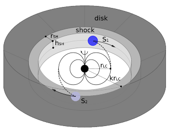
Figure 14: Schematic diagram of the pulsar wind scenario we propose to explain the optical and X-ray pulses observed from PSR J1023+0038. Dashed lines represent the current sheet which expands from the light cylinder surface at $r_{LC}$ as an Archimedean spiral. Its arms crosses the termination shock (shaded in light gray) at S₁ and S₂ where particles are accelerated to relativistic energies. As long as the particle energy is quickly radiated away and the size of the shock is smaller than a few light cylinder radii, two bright synchrotron-emitting spots (drawn in blue) rotate at the shock surface. An observer will see pulses of radiation because the intensity received from S₁ is modulated by the angle under which the spot is seen, and the emission coming from S₂ is absorbed by the optically thick disk in-flow (shaded in dark gray).

Close to the light cylinder the spin down energy of the pulsar is transported outwards by the electromagnetic field. In the striped wind model, the magnetic field configuration has the shape of two monopoles of opposite polarity which join at the equatorial plane (Bogovalov, 1999) and a current sheet forms along such a plane where the field changes polarity. In the oblique rotator case, the rotation of the pulsar introduces oscillations in the the current sheet which expands as an Archimedean spiral whose arms are separated by $\pi r_{LC}=cP_{s}/2$ (see Fig. 4 of Bogovalov, 1999). Injection of energy at the termination intrabinary shock then proceeds with a periodicity of $\sim P_{s}/2$. The electrons accelerated to relativistic energies at different locations in the shock will radiate their energy on a time scale

$$\begin{split}t_{sync}&\simeq\frac{\gamma m_{e}c^{2}}{P_{sync}}\simeq\frac{9m_{e}^{3}c^{5}}{4e^{4}B_{s}^{2}\gamma}\\ &\simeq 1.8\,\left(\frac{\epsilon}{10~{}\mbox{keV}}\right)^{-1/2}\,\left(\frac{B_{s}}{4.5\times 10^{5}~{}\mbox{G}}\right)^{-3/2}\,\mu\mbox{s}\end{split}$$ (7)

where we used the relations, $P_{sync}\simeq 4/3\,\sigma_{T}c\gamma^{2}U_{B}$ for the synchrotron power emitted by a relativistic electron and $\epsilon=0.29(3e\hbar/2m_{e}c)B_{s}\gamma^{2}$ (Ginzburg & Syrovatskij, 1965) to express the energy of photons at which most of the synchrotron power is emitted in terms of the electron energy $\gamma m_{e}c^{2}$. In the expressions above, $\sigma_{T}=8\pi e^{4}/3m_{e}^{2}c^{4}$ is the Thomson scattering cross section and $U_{B}=B^{2}/8\pi$ is the magnetic energy density. On the other hand, the light travel time between different regions of the shock is:

$$t_{lt}=2kr_{LC}\sin{i}/c=kP_{S}\sin{i}/\pi=533\,k\sin{i}\,\mu\mbox{s}.$$ (8)

As long as both the emission time scale and the light travel time between different locations of the emission regions are shorter than, say, half the spin period, a synchrotron emitting spot (shaded in blue in Fig. 14) will be seen to rotate coherently at the shock surface with a period $P_{S}/2$. For a moderately large inclination angle, the exact value depending on the disk and shock relative height, the disk will absorb the emission coming from the spot closest to the observer (labeled as $S_{2}$ in Fig. 14). On the other hand, the emission from the spot located farther from the observer ($S_{1}$) will be modulated sinusoidally as the spot rotates, as if the wind-disk shock were a sort of reflecting mirror. Two pulses of optical/Xray synchrotron radiation will be then observed every spin cycle of the pulsar, whose relative amplitude depends on the magnetic inclination angle, as well as on the viewing angle. Relativistic beaming and/or an ordered magnetic field would increase the anisotropy of the emitted radiation and the pulse amplitude. In this scenario, the large duty cycle of the observed X-ray pulse could result from the sum of the periodic emission emitted from different locations of the intrabinary shock, which are reached at the different times by the spiralling-out current sheet, and are seen at different angles from the observer. Interestingly, the synchrotron timescale for optical photons is $\sim 180\,\mu$s, compatible with the lag of optical pulses with respect to X-rays. The observed lag would find an immediate interpretation in our modeling, as optical synchrotron photons take a longer time to be emitted than X-rays.

The synchrotron timescale expressed by Eq. 7 increases if the shock is located at a greater distance because the strength of the post-shock magnetic field decreases linearly with distance (see Eq. 6). Eventually, it becomes comparable to half the spin period for 1 eV photons when the magnetic field at the shock is as low as $1.5\times 10^{5}$ G. To produce optical coherent oscillations the shock surface must be then located at $k\lower 2.15277pt\hbox{$\;\buildrel<\over{\sim}\;$}2$ times the light cylinder radius. The condition of the light travel time of different regions of the shock, $\approx 2kr_{LC}\sin{i}/c=kP_{s}/2\pi<P_{s}/2$, implies a similar constraint, $k<\pi/(2\sin{i})$. Remarkably, the latter condition is geometrical and does not depend on the energy of the photons. We speculate that the simultaneous disappearance of X-ray and optical pulses during the low mode might be due to the inner rings of the mass inflow being pushed outwards by the pulsar wind, corresponding to an expansion of the termination radius beyond $\simeq\pi/(2\sin{i})$ ($k\simeq 2.2$ for $i=45^{\circ}$) times the light cylinder radius. This is in agreement with the observation of radio flares during the X-ray low modes by Bogdanov et al. (2018), who interpreted them as episodes of ejection of optically thin plasmoids by the rotation-powered pulsar.

The synchrotron emission timescale expressed by Eq. 7 is shorter than the flight time of accelerated particles in the shock region, $r_{SH}/c\simeq 33\,(r_{SH}/10\mbox{km})\,\mu$s, provided that the latter is larger than a few km. This ensures that the energy of the electrons is radiated away before they escape from the acceleration region.

The energy radiated in pulsed X-rays is $5\times 10^{-3}$ times the spin down energy. The X-ray efficiency of typical isolated pulsar wind nebulae is usually of a few per cent of the spin down power (Kargaltsev & Pavlov, 2010), and rarely reaches a value larger than ten per cent out of the reverberation phase (Younes et al., 2016; Torres & Lin, 2018). Assuming an efficiency of the order of that observed from the Crab pulsar nebula (0.04), roughly $10\%$ of the pulsar wind energy must be converted into X-rays to match the pulsed flux observed from PSR J1023+0038. For an isotropic distribution of the pulsar wind, the shock height must be $h_{SH}\sim 0.2kr_{LC}$ to meet the energy requirement. This is ten times larger than the height a Keplerian disk would have at a similar distance for a mass accretion rate $\dot{m}_{14}$, indicating that the shock must be vertically extended. An even more extended shock is required if the whole X-ray luminosity seen in the high mode ($\simeq 0.2\dot{E}$) is due to synchrotron emission in the intrabinary shock, suggesting a higher efficiency of conversion of the pulsar wind in electron energy than previously assumed. A detailed modeling of the multi-wavelength spectral energy distribution of PSR J1023+0038, including also the component observed at GeV energies will be presented in a forthcoming paper.

In the context of a variable shock height $h_{SH}$, an increase of the solid angle covered by the shock could explain flares observed simultaneously in the optical and X-ray bands. As these sometimes reach a luminosity comparable to the spin down power of PSR J1023+0038 (Bogdanov et al., 2015), it is evident that almost complete enshrouding of the pulsar by disk plasma and a conversion efficiency of spin down power into electron energy close to unity would be required. It is unclear, however, why X-ray pulsations should disappear during flares. As we pointed out earlier, the non-detection could be due to the lower counting statistics in the X-ray band than in the optical band. The pulsed optical luminosity observed during flares is roughly a third of that observed in the high mode; a smaller decrease of the amplitude would be expected if flares were a sheer superimposition of unpulsed flux over the high mode level. In addition, we observed a similar decrease in the optical pulse amplitude in intervals that formally fell in the high mode according to our definition, but were observed in-between flares (i.e. towards the end of TNG2, see Fig. 3). This would suggest that flaring intervals unlikely result from the addition of a component to the high mode emission, and should be treated separately. However, it is also possible that flares are produced in the outer regions of the disk, and the marked decrease of the optical pulse amplitude during flares could be due to the occurrence of low modes that cannot be identified from the X-ray light curve as they are out-shined by the flaring emission. More observations of the pulsed amplitude decrease during flares are needed to break the degeneracy and identify the region where flares are produced.

The possibility that the accretion flow is stopped by the pulsar wind just beyond the light cylinder by the pulsar wind was recently explored with general relativistic MHD simulations by Parfrey & Tchekhovskoy (2017, see panel d in their Fig. 4), who noted that X-ray emission would be expected from the trains of shocks and sound waves produced at the pulsar wind termination. They found that in this scenario the amount of open magnetic flux was similar to the isolated pulsar case. The spin down rate of the pulsar was then expected to be similar to that observed in the rotation-powered state. This is qualitatively in agreement with the $\sim 30\%$ increase in the spin down rate observed by J16 after the formation of an accretion disk, a factor much smaller than that expected if accretion and/or propeller ejection took place.

Ekşİ & Alpar (2005) showed that a stable equilibrium between the outward pressure of a rotation-powered pulsar and the inward pressure of the infalling matter can be realized if the termination shock is close to the light cylinder; this is due to the presence of a transition region from the near region inside the light cylinder, where the energy density of the electromagnetic field scales as $\sim r^{-6}$, to the radiation zone far outside the light cylinder, where the $\sim r^{-2}$ scaling holds. Equilibrium solutions for values of the disk truncation radius $kr_{LC}$ with $k\lower 2.15277pt\hbox{$\;\buildrel>\over{\sim}\;$}1$ were found, the exact value depending on the angle between the magnetic moment and the rotation axis, $1-\alpha$. For instance, they found stable solutions with $1<k<2$ for $\xi=10^{\circ}$ and $\mu_{26}=1$, compatible with the assumptions of our model. On the other hand, far from the light cylinder the radiation of a rotation-powered pulsar ($\sim r^{-2}$) decreases less steeply than the ram pressure of matter in-falling under the gravitational pull of the compact object ($\sim r^{-5/2}$). Because of this, a stable solution of a rotation-powered pulsar surrounded by an accretion disk would not ensue as the disk is expected to be fully ablated away by the pulsar wind as soon as $r_{m}>>r_{LC}$ (Shvartsman, 1970; Burderi et al., 2001). Takata et al. (2014) and Coti Zelati et al. (2014) modeled the multi-wavelength emission of PSR J1023+0038 assuming that the rotation-powered pulsar wind interacted with the accretion disk to produce synchrotron X-ray emission far from the light cylinder ($\sim 10^{9}$ cm, i.e. $k\sim 125$). Besides the problems of stability that would probably ensue, we note that in the framework we propose coherent pulsations would not be produced at such a large distance from the pulsar.

Assuming that most of the pulsed emission is produced at the intrabinary shock between the pulsar wind and the disk does not rule out that magnetospheric rotation-powered pulses are still produced at a similar level than observed during the radio-pulsar state. However, even if a radio pulsar were active, its pulses would be smeared and absorbed by material ejected by the pulsar wind (Stappers et al., 2014). On the other hand, the five-fold increase in gamma-ray flux observed after the disk formation could be due to Compton up-scattering of disk UV photons off the cold relativistic pulsar wind, as proposed by Takata et al. (2014), while the pulsed magnetospheric emission keeps working at a similar rate as in the radio pulsar state (Tam et al., 2010).

5 Conclusions

We presented the first simultaneous optical and X-ray high temporal resolution observations of PSR J1023+0038 in the accretion disk state, the only optical millisecond pulsar discovered so far (Ambrosino et al., 2017). We showed that optical pulsations are detected during the high mode observed in the X-ray light curve, in which also X-ray pulsations appear, while pulsations in both bands disappear in the low mode. Optical pulses are described by two harmonics, similar to X-ray pulses and lag the X-ray pulses by $\sim 200\,\mu$s, although we caution that the absolute time calibration of SiFAP is based on just a single observations (see A1). These findings suggest that the same phenomenon produces the pulses seen in both energy bands. Cyclotron emission from matter accreting onto the polar caps of the NS is not powerful enough to explain the pulsed optical luminosity. On the other hand, emission from the magnetosphere of a rotation-powered pulsar requires an unusually large efficiency of spin down power conversion to match the optical and X-ray pulsed flux of PSR J1023+0038 with respect to other known pulsars. We argued that PSR J1023+0038 is a rotation-powered pulsar whose relativistic, highly magnetized wind interacts with the inflowing disk matter just beyond the light cylinder, creating a shock where the wind periodically deposits energy by accelerating electrons at the shock; these in turn produce optical and X-ray pulses through synchrotron emission. This would make PSR J1023+0038 the prototype of a few hundred km-sized pulsar wind nebula, and provide an unique opportunity to study the pulsar wind properties in the high magnetization regime rather than where they are particle-dominated, as in the usual sub-parsec scale pulsar wind nebulae. This scenario also provides an explanation of the low mode and flares observed in the X-ray light curve in terms of the shock being pushed back by the pulsar radiation or increasing its size, respectively. Future observations will confirm the phase lag between optical and X-ray pulses, study the energy distribution of the pulses in the visible band, search for polarized pulsed emission, and look for gamma-ray pulsations, thus testing the scenario we proposed. On the other hand, magneto-hydrodynamic simulations will be performed to demonstrate that pulsed emission can be indeed generated by a disk/wind intrabinary shock close to the light cylinder of a pulsar. The stability of a wind-disk shock just beyond the light cylinder over timescales of years should also be investigated. Other transitional millisecond pulsars in the sub-luminous disk state such as XSS J12270-4859 (de Martino et al., 2010, 2013; Bassa et al., 2014) and candidates like 1RXS J154439.4–112820 (Bogdanov & Halpern, 2015) ans 1SXPS J042947.1–670320 (Strader et al., 2016), XMM J083850.4–282759 (Rea et al., 2017) and CXOU J110926.4-650224 (Coti Zelati et al., 2019) may be found in a similar state to that PSR J1023+0038. A search of optical pulsations in those source seems therefore warranted.

Appendix A SiFAP observations of the Crab PSR

We observed the Crab PSR with SiFAP at the 152 cm Cassini Telescope at Loiano Observatory for 3.3 ks starting on $T_{0}=$57724.04514 MJD. The target was observed at an average count rate of $45\times 10^{3}$ s^-1. We reduced data following the same steps described in Sec. 2.6, correcting the arrival times for the assumed linear SiFAP clock drift, and reporting them to the Solar System barycenter using the software Tempo2 (Hobbs et al., 2006), considering the position (RA $05^{h}$ $34^{m}$ $31.97232^{s}$ , Dec $+22^{\circ}$ 00’ $52.0690^{\prime\prime}$ [J2000]) and the JPL DE200 ephemerides used by the Jodrell Bank monthly ephemerides (Lyne et al., 1993). We epoch folded the optical time series in 1024 phase bins using the epoch of the nearest arrival time of the main pulse, $T_{JB}=57715.000000195995$ MJD, the period $0.03372925321514(43)$ s and the period derivative $4.197644(15)\times 10^{-18}$. The maximum of the main pulse occurs at phase $\delta\phi_{Crab}=-0.0054\pm 0.0005$ (see Fig. 15). Considering the uncertainty reported in the Jodrell Bank ephemerides is 60$\mu$ s, we then estimate that the optical pulse lag the radio one by $\delta\tau_{Crab}=(181\pm 62)\,\mu$s. This is compatible with the estimates given by Oosterbroek et al. (2008), who quoted $(255\pm 21)\,\mu$s from simultaneous optical and radio timing, Germanà et al. (2012, $\delta\tau\simeq 230\,\mu$s), Collins et al. (2012, $\delta\tau\sim 178\mu$s) and Zampieri et al. (2014, $\delta\tau\sim 240\mu$s). We then conclude that the absolute timing accuracy of SiFAP is better than 60$\mu$s.

Figure 15: Pulse profile of the Crab pulsar observed with SiFAP at the Cassini Telescope at Loiano Observatory. Zero epoch corresponds to the nearest Jodrell Bank radio main pulse epoch $T_{JB}=57715.000000195995$ MJD. The profile was obtained folding the SiFAP time series in 1024 time bins using the period $0.03372925321514(43)$ s and the period derivative $4.197644(15)\times 10^{-18}$ evaluated at $T_{JB}$. The inset shows a magnification of the peak. Vertical dotted lines indicate the phase of optical and radio maximum.

A.1 The optical flux

To determine the optical flux of PSR J1023+0038 during the SiFAP/TNG observations we first calibrated the flux/count-rate conversion factor, $k$. The count rate observed by SiFAP is expressed by:

$$R=C\times\int\frac{\lambda F_{\lambda}(\lambda)}{hc}A_{e}R(\lambda)E(\lambda)d\lambda,$$ (A1)

where $F_{\lambda}(\lambda)$ is the flux density, $A_{e}=9\times 10^{4}$ cm² is the effective area of the TNG mirror, $R(\lambda)$ is the response of the detector equipped with a white filter (see Supplementary Fig.1 in Ambrosino et al. 2017), and $E(\lambda)$ is the atmospheric extinction (we considered an air-mass of 2.0 and 1.3 for TNG1 and TNG2, respectively). We measured the normalization factor $C$ by evaluating Eq. A1 for the reference star; we calculated the integral for the synthetic spectrum of a G2 V star (Pickles & Depagne, 2010), normalized to give the observed flux density over the Sloan Digital Sky Service g filter ($g=15.86(1)$ mag, corresponding to $2.13\times 10^{-14}$ erg cm² nm^-1[=$1.64$ mJy]), and we matched it to the observed, background-subtracted count rate ($R_{REF,TNG1}=19456.8$ s^-1, $R_{REF,TNG2}=30750.2$ s^-1), obtaining $C_{TNG1}=0.434$ and $C_{TNG2}=0.686$. We attribute the difference between the normalization factors to the different atmospheric conditions over the two nights. The conversion factor $k$ for PSR J1023+0038 was then estimated as:

$$k=\frac{F_{J1023}}{R}=\frac{F_{J1023,NOT}}{C\times\int\frac{\lambda f_{\lambda,NOT}(\lambda)}{hc}A_{e}R(\lambda)E(\lambda),d\lambda}$$ (A2)

yielding $k_{1}=5.17\times 10^{-16}$ erg cm^-2 and $k_{2}=3.25\times 10^{-16}$ erg cm^-2 for TNG1 and TNG2, respectively. The rightmost column of Tab. 2 lists the 320-900 nm flux measured in the different modes by scaling the net observed count rates using these conversion factors and considering a 5% uncertainty. The de-reddened flux in the 320–900 nm band is a factor 1.22 larger than those values, considering the absorption column measured by Coti Zelati et al. (2014, $N_{H}=5.2\times 10^{20}$ cm^-2) a ratio $A_{V}/E(B-V)=3.1$, and the resulting color excess $E(B-V)=0.073$ (Predehl & Schmitt, 1995). We checked that performing this procedure to evaluate the ratio of the flux of PSR J1023+0038 and the reference star integrated over a B filter during the interval simultaneous to the TJO observation performed with the same filter (see Table 1), $F_{J1023}/F_{REF}=0.43$, is compatible with the flux ratio 0.41(2) indicated by the magnitudes observed ($B_{PSR}=17.10(3)$ mag, $B_{REF}=16.20(1)$ mag, $F_{J1023,TJO}/F_{REF,TJO}=0.44\pm 0.02$).

References

- Aliu et al. (2016) Aliu, E., Archambault, S., Archer, A., et al. 2016, Astrophys. J., 831, 193
- Ambrosino et al. (2016) Ambrosino, F., Cretaro, P., Meddi, F., et al. 2016, Journal of Astronomical Instrumentation, 5, 1650005
- Ambrosino et al. (2017) Ambrosino, F., Papitto, A., Stella, L., et al. 2017, Nature Astronomy, 1, 854
- Archibald et al. (2010) Archibald, A. M., Kaspi, V. M., Bogdanov, S., et al. 2010, Astrophys. J., 722, 88
- Archibald et al. (2013) Archibald, A. M., Kaspi, V. M., Hessels, J. W. T., et al. 2013, ArXiv e-prints, arXiv:1311.5161
- Archibald et al. (2009) Archibald, A. M., Stairs, I. H., Ransom, S. M., et al. 2009, Science, 324, 1411
- Archibald et al. (2015) Archibald, A. M., Bogdanov, S., Patruno, A., et al. 2015, Astrophys. J., 807, 62
- Arons (2002) Arons, J. 2002, in Astronomical Society of the Pacific Conference Series, Vol. 271, Neutron Stars in Supernova Remnants, ed. P. O. Slane & B. M. Gaensler, 71
- Arons & Tavani (1993) Arons, J., & Tavani, M. 1993, Astrophys. J., 403, 249
- Baglio et al. (2016) Baglio, M. C., D’Avanzo, P., Campana, S., et al. 2016, Astron. and Astrophys., 591, A101
- Basko & Sunyaev (1976) Basko, M. M., & Sunyaev, R. A. 1976, MNRAS, 175, 395
- Bassa et al. (2014) Bassa, C. G., Patruno, A., Hessels, J. W. T., et al. 2014, MNRAS, 441, 1825
- Bednarek (2015) Bednarek, W. 2015, MNRAS, 451, L55
- Bogdanov & Halpern (2015) Bogdanov, S., & Halpern, J. P. 2015, ApJ, 803, L27
- Bogdanov et al. (2015) Bogdanov, S., Archibald, A. M., Bassa, C., et al. 2015, Astrophys. J., 806, 148
- Bogdanov et al. (2018) Bogdanov, S., Deller, A. T., Miller-Jones, J. C. A., et al. 2018, Astrophys. J., 856, 54
- Bogovalov (1999) Bogovalov, S. V. 1999, Astron. and Astrophys., 349, 1017
- Bozzo et al. (2018) Bozzo, E., Ascenzi, S., Ducci, L., et al. 2018, Astron. and Astrophys., 617, A126
- Burderi et al. (2001) Burderi, L., Possenti, A., D’Antona, F., et al. 2001, ApJ, 560, L71
- Campana et al. (2016) Campana, S., Coti Zelati, F., Papitto, A., et al. 2016, Astron. and Astrophys., 594, A31
- Campana & Di Salvo (2018) Campana, S., & Di Salvo, T. 2018, ArXiv e-prints, arXiv:1804.03422
- Collins et al. (2012) Collins, S., Shearer, A., Stappers, B., et al. 2012, in IAU Symposium, Vol. 285, New Horizons in Time Domain Astronomy, ed. E. Griffin, R. Hanisch, & R. Seaman, 296–298
- Coti Zelati et al. (2018) Coti Zelati, F., Campana, S., Braito, V., et al. 2018, Astron. and Astrophys., 611, A14
- Coti Zelati et al. (2014) Coti Zelati, F., Baglio, M. C., Campana, S., et al. 2014, MNRAS, 444, 1783
- Coti Zelati et al. (2019) Coti Zelati, F., Papitto, A., de Martino, D., et al. 2019, Astron. and Astrophys., 622, A211
- D’Amico et al. (2001) D’Amico, N., Possenti, A., Manchester, R. N., et al. 2001, ApJ, 561, L89
- D’Angelo & Spruit (2012) D’Angelo, C. R., & Spruit, H. C. 2012, MNRAS, 420, 416
- de Martino et al. (2010) de Martino, D., Falanga, M., Bonnet-Bidaud, J.-M., et al. 2010, Astron. and Astrophys., 515, A25
- de Martino et al. (2013) de Martino, D., Belloni, T., Falanga, M., et al. 2013, Astron. and Astrophys., 550, A89
- Deller et al. (2012) Deller, A. T., Archibald, A. M., Brisken, W. F., et al. 2012, ApJ, 756, L25
- Deller et al. (2015) Deller, A. T., Moldon, J., Miller-Jones, J. C. A., et al. 2015, Astrophys. J., 809, 13
- Ekşİ & Alpar (2005) Ekşİ, K. Y., & Alpar, M. A. 2005, Astrophys. J., 620, 390
- Ferrigno et al. (2014) Ferrigno, C., Bozzo, E., Papitto, A., et al. 2014, Astron. and Astrophys., 567, A77
- Frank et al. (2002) Frank, J., King, A., & Raine, D. J. 2002, Accretion Power in Astrophysics: Third Edition, 398
- Gendreau et al. (2012) Gendreau, K. C., Arzoumanian, Z., & Okajima, T. 2012, in Proc. SPIE, Vol. 8443, Space Telescopes and Instrumentation 2012: Ultraviolet to Gamma Ray, 844313
- Germanà et al. (2012) Germanà, C., Zampieri, L., Barbieri, C., et al. 2012, Astron. and Astrophys., 548, A47
- Ginzburg & Syrovatskij (1965) Ginzburg, V. L., & Syrovatskij, S. I. 1965, Sp.Sc.Rev., 4, 267
- Goldreich & Julian (1969) Goldreich, P., & Julian, W. H. 1969, Astrophys. J., 157, 869
- Hakala & Kajava (2018) Hakala, P., & Kajava, J. J. E. 2018, MNRAS, 474, 3297
- Hermsen et al. (2013) Hermsen, W., Hessels, J. W. T., Kuiper, L., et al. 2013, Science, 339, 436
- Hobbs et al. (2006) Hobbs, G. B., Edwards, R. T., & Manchester, R. N. 2006, MNRAS, 369, 655
- Jaodand et al. (2016) Jaodand, A., Archibald, A. M., Hessels, J. W. T., et al. 2016, Astrophys. J., 830, 122
- Kargaltsev & Pavlov (2010) Kargaltsev, O., & Pavlov, G. G. 2010, X-ray Astronomy 2009; Present Status, Multi-Wavelength Approach and Future Perspectives, 1248, 25
- Kennedy et al. (2018) Kennedy, M. R., Clark, C. J., Voisin, G., & Breton, R. P. 2018, MNRAS, 477, 1120
- Kennel & Coroniti (1984) Kennel, C. F., & Coroniti, F. V. 1984, Astrophys. J., 283, 710
- Lamb & Masters (1979) Lamb, D. Q., & Masters, A. R. 1979, ApJ, 234, L117
- Lee et al. (2018) Lee, J., Hui, C. Y., Takata, J., et al. 2018, Astrophys. J., 864, 23
- Lefa et al. (2012) Lefa, E., Kelner, S. R., & Aharonian, F. A. 2012, Astrophys. J., 753, 176
- Li et al. (2018) Li, J., Torres, D. F., Coti Zelati, F., et al. 2018, arXiv e-prints, arXiv:1811.08339
- Li et al. (2014) Li, K. L., Kong, A. K. H., Takata, J., et al. 2014, Astrophys. J., 797, 111
- Linares (2014) Linares, M. 2014, Astrophys. J., 795, 72
- Lyne et al. (1993) Lyne, A. G., Pritchard, R. S., & Graham-Smith, F. 1993, MNRAS, 265, 1003
- Madsen et al. (2015) Madsen, K. K., Harrison, F. A., Markwardt, C. B., et al. 2015, ApJS, 220, 8
- Martín et al. (2012) Martín, J., Torres, D. F., & Rea, N. 2012, MNRAS, 427, 415
- Martin-Carrillo et al. (2012) Martin-Carrillo, A., Kirsch, M. G. F., Caballero, I., et al. 2012, Astron. and Astrophys., 545, A126
- Masters et al. (1977) Masters, A. R., Pringle, J. E., Fabian, A. C., & Rees, M. J. 1977, MNRAS, 178, 501
- Meddi et al. (2012) Meddi, F., Ambrosino, F., Nesci, R., et al. 2012, PASP, 124, 448
- Mereghetti et al. (2016) Mereghetti, S., Kuiper, L., Tiengo, A., et al. 2016, Astrophys. J., 831, 21
- Mignani (2011) Mignani, R. P. 2011, Advances in Space Research, 47, 1281
- O’Brien et al. (2002) O’Brien, K., Horne, K., Hynes, R. I., et al. 2002, MNRAS, 334, 426
- Oosterbroek et al. (2008) Oosterbroek, T., Cognard, I., Golden, A., et al. 2008, Astron. and Astrophys., 488, 271
- Pacini & Salvati (1983) Pacini, F., & Salvati, M. 1983, Astrophys. J., 274, 369
- Papitto et al. (2015) Papitto, A., de Martino, D., Belloni, T. M., et al. 2015, MNRAS, 449, L26
- Papitto et al. (2011) Papitto, A., Riggio, A., Burderi, L., et al. 2011, Astron. and Astrophys., 528, A55
- Papitto & Torres (2015) Papitto, A., & Torres, D. F. 2015, Astrophys. J., 807, 33
- Papitto et al. (2014) Papitto, A., Torres, D. F., & Li, J. 2014, MNRAS, 438, 2105
- Papitto et al. (2013) Papitto, A., Ferrigno, C., Bozzo, E., et al. 2013, Nature, 501, 517
- Papitto et al. (2018) Papitto, A., Rea, N., Coti Zelati, F., et al. 2018, ApJ, 858, L12
- Parfrey & Tchekhovskoy (2017) Parfrey, K., & Tchekhovskoy, A. 2017, ApJ, 851, L34
- Patruno & Watts (2012) Patruno, A., & Watts, A. L. 2012, ArXiv e-prints, arXiv:1206.2727
- Patruno et al. (2014) Patruno, A., Archibald, A. M., Hessels, J. W. T., et al. 2014, ApJ, 781, L3
- Percival et al. (1993) Percival, J. W., Biggs, J. D., Dolan, J. F., et al. 1993, Astrophys. J., 407, 276
- Pickles & Depagne (2010) Pickles, A., & Depagne, É. 2010, PASP, 122, 1437
- Possenti et al. (2002) Possenti, A., Cerutti, R., Colpi, M., & Mereghetti, S. 2002, Astron. and Astrophys., 387, 993
- Predehl & Schmitt (1995) Predehl, P., & Schmitt, J. H. M. M. 1995, Astron. and Astrophys., 293, 889
- Rea et al. (2017) Rea, N., Coti Zelati, F., Esposito, P., et al. 2017, MNRAS, 471, 2902
- Roberts et al. (2018) Roberts, M. S. E., Al Noori, H., Torres, R. A., et al. 2018, in IAU Symposium, Vol. 337, Pulsar Astrophysics the Next Fifty Years, ed. P. Weltevrede, B. B. P. Perera, L. L. Preston, & S. Sanidas, 43–46
- Romani (1996) Romani, R. W. 1996, Astrophys. J., 470, 469
- Romanova et al. (2004) Romanova, M. M., Ustyugova, G. V., Koldoba, A. V., & Lovelace, R. V. E. 2004, Astrophys. J., 610, 920
- Rybicki & Lightman (1979) Rybicki, G. B., & Lightman, A. P. 1979, Radiative processes in astrophysics
- Shahbaz et al. (2018) Shahbaz, T., Dallilar, Y., Garner, A., et al. 2018, MNRAS, 477, 566
- Shahbaz et al. (2015) Shahbaz, T., Linares, M., Nevado, S. P., et al. 2015, MNRAS, 453, 3461
- Shvartsman (1970) Shvartsman, V. F. 1970, SvA, 14, 527
- Shvartsman (1971) —. 1971, SvA, 15, 342
- Spitkovsky (2006) Spitkovsky, A. 2006, ApJ, 648, L51
- Stappers et al. (2014) Stappers, B. W., Archibald, A. M., Hessels, J. W. T., et al. 2014, Astrophys. J., 790, 39
- Strader et al. (2016) Strader, M. J., Archibald, A. M., Meeker, S. R., et al. 2016, MNRAS, 459, 427
- Takata et al. (2014) Takata, J., Li, K. L., Leung, G. C. K., et al. 2014, Astrophys. J., 785, 131
- Tam et al. (2010) Tam, P. H. T., Hui, C. Y., Huang, R. H. H., et al. 2010, ApJ, 724, L207
- Tendulkar et al. (2014) Tendulkar, S. P., Yang, C., An, H., et al. 2014, Astrophys. J., 791, 77
- Tody (1986) Tody, D. 1986, in Proc. SPIE, Vol. 627, Instrumentation in astronomy VI, ed. D. L. Crawford, 733
- Torres (2018) Torres, D. F. 2018, Nature Astronomy, 2, 247
- Torres et al. (2017) Torres, D. F., Ji, L., Li, J., et al. 2017, Astrophys. J., 836, 68
- Torres & Lin (2018) Torres, D. F., & Lin, T. 2018, ApJ, 864, L2
- Trubnikov (1958) Trubnikov, B. A. 1958, PhD thesis, Dissertation, Moscow (US-AEC Tech. Inf. Service, AEC-tr-4073 [1960]), (1958)
- Veledina et al. (2019) Veledina, A., Nättilä, J., & Beloborodov, A. M. 2019, arXiv e-prints, arXiv:1906.02519
- Venter et al. (2018) Venter, C., Harding, A. K., & Grenier, I. 2018, ArXiv e-prints, arXiv:1802.00204
- Viganò et al. (2015) Viganò, D., Torres, D. F., Hirotani, K., & Pessah, M. E. 2015, MNRAS, 447, 1164
- Vink et al. (2011) Vink, J., Bamba, A., & Yamazaki, R. 2011, Astrophys. J., 727, 131
- Wang et al. (2009) Wang, Z., Archibald, A. M., Thorstensen, J. R., et al. 2009, Astrophys. J., 703, 2017
- Wijnands & van der Klis (1998) Wijnands, R., & van der Klis, M. 1998, Nature, 394, 344
- Younes et al. (2016) Younes, G., Kouveliotou, C., Kargaltsev, O., et al. 2016, Astrophys. J., 824, 138
- Zacharias et al. (2013) Zacharias, N., Finch, C. T., Girard, T. M., et al. 2013, AJ, 145, 44
- Zampieri et al. (2014) Zampieri, L., Čadež, A., Barbieri, C., et al. 2014, MNRAS, 439, 2813
- Zavlin (2007) Zavlin, V. E. 2007, Ap&SS, 308, 297