Guaranteed and robust $L_{2}$-norm a posteriori error estimates for 1D linear advection problems

Abstract

We propose a reconstruction-based a posteriori error estimate for linear advection problems in one space dimension. In our framework, a stable variational ultra-weak formulation is adopted, and the equivalence of the $L_{2}$-norm of the error with the dual graph norm of the residual is established. This dual norm is showed to be localizable over vertex-based patch subdomains of the computational domain under the condition of the orthogonality of the residual to the piecewise affine hat functions. We show that this condition is valid for some well-known numerical methods including continuous/discontinuous Petrov–Galerkin and discontinuous Galerkin methods. Consequently, a well-posed local problem on each patch is identified, which leads to a global conforming reconstruction of the discrete solution. We prove that this reconstruction provides a guaranteed upper bound on the $L_{2}$ error. Moreover, up to a constant, it also gives local lower bounds on the $L_{2}$ error, where the generic constant is proven to be independent of mesh-refinement, polynomial degree of the approximation, and the advective velocity. This leads to robustness of our estimates with respect to the advection as well as the polynomial degree. All the above properties are verified in a series of numerical experiments, additionally leading to asymptotic exactness. Motivated by these results, we finally propose a heuristic extension of our methodology to any space dimension, achieved by solving local least-squares problems on vertex-based patches. Though not anymore guaranteed, the resulting error indicator is numerically robust with respect to both advection velocity and polynomial degree, for a collection of two-dimensional test cases including discontinuous solutions.

Key words: linear advection problem; discontinuous Galerkin method; Petrov–Galerkin method; a posteriori error estimate; local efficiency; advection robustness; polynomial-degree robustness

1 Introduction

This work deals with a linear advection equation of the form: find $u:\Omega\subset\mathbb{R}^{d}\rightarrow\mathbb{R}$ such that

$${\bm{b}}{\cdot}{\nabla u}=f, \qquad\text{ in }\Omega,$$ (1.1a)

$$u=0, \qquad\text{ on }\partial_{-}\Omega.$$ (1.1b)

The velocity field $\bm{b}\in\mathcal{C}^{1}(\overline{\Omega};\mathbb{R}^{d})$, $\bm{b}\neq 0$, is considered to be divergence-free and we take into account a general source term $f\in L_{2}(\Omega)$. The inflow, outflow, and characteristic parts of the boundary are denoted by $\partial_{-}\Omega,\partial_{+}\Omega$, and $\partial_{0}\Omega$, respectively, with the definitions

$$\partial_{\pm}\Omega\vcentcolon=\{x\in\partial\Omega:\pm\bm{b}(x){\cdot}\bm{n}(x)>0\},\qquad\partial_{0}\Omega\vcentcolon=\{x\in\partial\Omega:\bm{b}(x){\cdot}\bm{n}(x)=0\}.$$

In the main body of the paper, we focus on the one-dimensional case $d=1$, where $\Omega\subset\mathbb{R}$ is a bounded simply connected interval; then $\bm{b}$ is a constant scalar. We keep the notations in multi-dimensional form in order to be applicable when we discuss extensions of our results to the multi-dimensional case.

The a posteriori error analysis for problem (1.1) admits a range of functional frameworks and consequently different norms in which the error can be measured. Our goal is to derive an $L_{2}$-norm error estimate of the form

$$\|u-u_{h}\|_{L_{2}(\Omega)}\leq\eta,$$ (1.2)

where $u$ is the weak solution of (1.1) in $L_{2}(\Omega)$, $u_{h}$ is its numerical approximation, and $\eta$ is an a posteriori error estimator fully computable from $u_{h}$ by some local procedure. We seek to have a bound that is guaranteed, i.e., featuring no unknown constant, in contrast to reliability where a bound up to a generic constant is sufficient. We develop a unified framework treating several classical numerical methods at once. Importantly, we also prove a converse estimate to (1.2) in the form

$$\eta\leq C\|u-u_{h}\|_{L_{2}(\Omega)}+\text{data oscillation}.$$ (1.3)

This is called global efficiency and yields equivalence between the incomputable error $\|u-u_{h}\|_{L_{2}(\Omega)}$ and the computable estimator $\eta$ up to the data oscillation term that vanishes for piecewise polynomial datum $f$ and that is of higher order than the error for piecewise smooth datum $f$. Crucially, in our developments, the generic constant $C$ in (1.3) only depends on the mesh shape regularity, requesting for $d=1$ each two neighboring elements to be of comparable size. In particular, $C$ is independent of the problem parameters $\bm{b}$ and $f$ as well as of the polynomial degree of the approximation $k$, yielding both data- and polynomial-degree-robustness. We actually also show local efficiency, i.e., a localized version of (1.3), which is highly desirable on the practical side in view of adaptive mesh refinement.

To achieve the above-mentioned goals, we start with the ultra-weak variational formulation at the infinite-dimensional level, where the solution lies in the $L_{2}(\Omega)$ trial space and the test space is formed by $H^{1}(\Omega)$ functions taking zero value at the outflow boundary. In this setting, we prove the equality of the $L_{2}$-norm of the error with the dual graph norm (relying on $\|{\bm{b}}{\cdot}{\nabla(\cdot)}\|_{L_{2}(\Omega)}$) of the residual. In the one-dimensional case, we are able to prove that the global dual norm can be localized over vertex-based patches of elements under an orthogonality condition against the hat basis functions. Consequently, suitable discrete local problems posed over these patches are identified which lead to local reconstructions $s_{h}^{\bm{a}}$ combined into a global reconstruction $s_{h}$ such that $\|u_{h}-s_{h}\|_{L_{2}(\Omega)}$ forms the main ingredient of the estimator $\eta$ satisfying (1.2) and (1.3).

Let us recall some important contributions to a posteriori error estimation for problem (1.1). Bey and Oden in [5] proposed an a posteriori error estimate for a discontinuous Galerkin (dG) formulation of the multi-dimensional advection–reaction problem. In this framework, two infinite-dimensional problems have to be solved on each mesh element; one to obtain the lower bound on the error and one for the upper bound, in two different and inequivalent weighted energy norms. This gives estimates similar to (1.2) and (1.3), but for two different estimators and in two different norms of the error. Additionally, one cannot solve analytically the infinite-dimensional elementwise problems, and, in practice, one needs to approximate them by some higher-order finite element approximation. Hence, neither simultaneous reliability and efficiency, nor robustness, are granted.

Süli in [29] applied the $H^{1}$-stability result of Tartakoff [31] to the adjoint problem of (1.1) (with the presence of the reaction term and in the multi-dimensional case), and obtained a global reliable upper bound on the $H^{-1}$-norm of the error in terms of the $L_{2}$-norm of the residual for a weak formulation of (1.1) with distinct trial and test spaces. He further turned this bound into a reliable $H^{-1}$-norm a posteriori error indicator for the streamline-diffusion finite element and the cell-vertex finite volume methods. However, neither the efficiency nor the robustness of this error indicator are discussed. Furthermore, in [29] by Süli and in [21] by Süli and Houston, an analysis of the multi-dimensional advection–reaction problem in the graph space equipped with the full norm $\|\cdot\|_{{L_{2}(\Omega)}}+\|{\bm{b}}{\cdot}{\nabla(\cdot)}\|_{{L_{2}(\Omega)}}$, is provided. This functional setting provides the equivalence between the $L_{2}$-norm of the error and the dual graph norm of the residual up to some generic constants, which is a weaker error–residual equivalence result compared to what we establish in the current work, see Theorem 2.1 below, upon replacing the full graph norm by $\|{\bm{b}}{\cdot}{\nabla(\cdot)}\|_{{L_{2}(\Omega)}}$ only. Overall, no complete reliability, efficiency, and robustness results of the form (1.2)–(1.3) are obtained.

Becker et al. in [4], derived reconstruction-based error estimators for the advection problem (1.1) in two space dimensions. An $\bm{H}(\mathrm{div},\Omega)$-conforming reconstruction is proposed for the flux vector $\bm{b}u$ (instead of $u$ in the present work) which is designed to produce a guaranteed upper bound on the error measured in some dual norm of the advection operator. A unified framework is built, covering the dG and conforming finite element methods with/without stabilization terms. This dual norm is hard to evaluate even for a known exact solution, and, in practice, the authors replace it by the $L_{2}$-norm, so that the guaranteed upper bound property is eventually lost. Proofs of efficiency or robustness are not given, but optimal convergence orders of the estimator are observed in numerical experiments. It is worth mentioning that, restricted to one space dimension, the dual norm of [4] reduces to the weak graph norm we employ. Our contribution in this respect consists in the proofs of (1.2) and (1.3), not given in [4] (where, recall, two space dimensions are treated.)

In a recent result by Georgoulis et al. in [19], the authors used the reconstruction proposed by Makridakis and Nochetto in [23] for a dG approximation and provided a reliable upper bound on the error in the energy norm for one-dimensional advection–diffusion–reaction problems, as well as a reliable $L_{2}$-norm estimate for the problem (1.1) in one space dimension. Though a proof of (1.3) is not given, efficiency and robustness are numerically observed. One might also note the earlier work of these authors [18], dedicated to the two-dimensional advection–reaction problem with a similar reconstruction. In that work, a reliable bound on the energy norm of the error is presented, though again without a theoretical elaboration on the efficiency and robustness.

Finally, let us mention the recent result of Dahmen and Stevenson in [12] where the authors provide a posteriori error estimates for the discontinuous Petrov–Galerkin method tailored to the transport equations in two space dimensions. The equivalence of the errors of the bulk and skeleton quantities with the dual norm of the residual is established. This dual norm is later approximated by some equivalent yet computable indicator. The absorbed constants translate into a constant $C$ in (1.3) which depends on the advective field $\bm{b}$ and the polynomial degree of approximation, therefore precluding the robustness of the error lower bound.

We also mention that in the case of advection–diffusion(–reaction) problems, other approaches were previously considered to obtain robustness with respect to the advective field. Among them, Verfürth [32] proposed to augment the energy norm by a dual norm coming from the skew-symmetric part of the differential operator, and Sangalli [25, 26] used interpolated spaces and a fractional-order norm for the advective term. Extensions of these approaches can be found in [27, 28, 15]. However, the above results are not applicable when the diffusion parameter vanishes, i.e., as the advection–diffusion problem reduces to (1.1) because the diffusive part of the operator is needed to evaluate the dual norm.

We treat problem (1.1) in one space dimension in Sections 2–8. Section 2 deals with the functional settings, whereby adopting the ultra-weak variational formulation. We prove, in particular, the equality of the $L_{2}$-norm of the error and the dual norm of the residual. Section 3 introduces some numerical schemes for approximating (1.1). Section 4 discusses the localization of the dual norm of the residual over vertex-based patches, showing in particular that this is possible for the schemes discussed in Section 3. In Section 5, we present our local patchwise reconstruction. Sections 6 and 7 then present the proofs for the upper and lower bounds as well as robustness in the form of (1.2)–(1.3). Section 8 then contains results of several numerical experiments to illustrate the developed theory. Finally, in Section 9, we consider the advection problem (1.1) in multiple space dimensions and derive a heuristic extension of our methodology to this case. Although we cannot prove here the guaranteed upper bound, (local) efficiency, and robustness, numerical experiments indicate appreciable properties of the derived estimates also in this case.

2 Abstract framework

We start with the presentation of the abstract framework.

2.1 Spaces

In the one-dimensional case, the constraint of $\bm{b}$ being a non-zero divergence-free field is translated to $\bm{b}$ being a constant nonzero scalar. Consequently, we are lead to work with the spaces

$$H^{1}_{-}(\Omega)=\left\{w\in H^{1}(\Omega),w=0,\text{ on }{\partial_{-}\Omega}\right\},\qquad H^{1}_{+}(\Omega)=\left\{w\in H^{1}(\Omega),w=0,\text{ on }{\partial_{+}\Omega}\right\}.$$ (2.1)

The trace operator in these spaces is well-defined and the following integration-by-parts formula holds:

$$(v,{\bm{b}}{\cdot}{\nabla w})_{\Omega}+({\bm{b}}{\cdot}{\nabla v},w)_{\Omega}=({\bm{b}}{\cdot}{\bm{n}}v,w)_{\partial\Omega},\qquad\forall v,w\in H^{1}(\Omega),$$ (2.2)

where the notation $(v,w)_{D}\vcentcolon=\int_{D}vw$ is used for an open subdomain $D\subseteq\Omega$ or its boundary $\partial D$ and for integrable functions $v$ and $w$. Henceforth, $\|v\|_{D}$ denotes the norm $\|v\|_{L_{2}(D)}=\sqrt{(v,v)_{D}}$. We will drop the subscript when $D=\Omega$.

2.2 Poincaré inequalities

The Poincaré inequality states that

$$\|v-\bar{v}\|_{D}\leq h_{D}C_{\mathrm{P},D}\|\nabla v\|_{D},\qquad\forall v\in H^{1}(D),$$ (2.3a)

with $$C_{\mathrm{P},D}>0 1/\pi D\subset\Omega \bar{v} v D \bar{v}=(v,1)_{D}/|D| h_{D} D$$ a generic constant, in particular equal to for convex . Here is the mean value of over defined as and is the diameter of . Similarly, another Poincaré inequality (sometimes called Friedrichs inequality) states that

$$\|v\|_{D}\leq h_{D}C_{\mathrm{P},D,\partial_{0}D}\|\nabla v\|_{D},\qquad\forall v\in\left\{H^{1}(D),v|_{\partial_{0}D}=0,|\partial_{0}D|\neq 0\right\},$$ (2.3b)

where $\partial_{0}D\subset\partial D$; typically $C_{\mathrm{P},D,\partial_{0}D}=1$. Henceforth, we will use $C_{\mathrm{PF},D}$ as a general notation for both $C_{\mathrm{P},D}$ and $C_{\mathrm{P},D,\partial_{0}D}$. It follows from the above that for a one-dimensional interval $D$, $C_{\mathrm{PF},D}$ can be taken as $1$.

2.3 Variational formulation and residual

The variational framework hinges upon an appropriate choice of the trial and test spaces and their corresponding norms. In particular, it turns out natural to work on spaces well-suited to the non-symmetric structure of the problem. Here we consider Hilbert spaces (non-symmetric formulations in Banach spaces can be found in [8, 24]).

The (usual) weak formulation of (1.1) reads: find $u\in H^{1}_{-}(\Omega)$ such that

$$({\bm{b}}{\cdot}{\nabla u},v)=(f,v),\qquad\forall v\in L_{2}(\Omega).$$ (2.4)

It is classically well-posed as one might confer with [17], [22], and [29, Proposition 6], cf.also [14] and [11, Rem. 2.2]. Here, we rather adopt the so-called ultra-weak formulation of problem (1.1) where the bilinear form is obtained by casting the derivatives on the test function, using integration-by-parts. It reads: find $u\in L_{2}(\Omega)$ such that

$$-(u,{\bm{b}}{\cdot}{\nabla v})=(f,v),\qquad\forall v\in H^{1}_{+}(\Omega).$$ (2.5)

The well-posedness of (2.5) can be shown by inf–sup arguments (cf. [14, Theorem 2.6] and [11, Theorem 2.4]).

Denote by $H^{1}_{+}(\Omega){{}^{\prime}}$ the dual space to $H^{1}_{+}(\Omega)$. For an arbitrary $u_{h}\in L_{2}(\Omega)$, the formulation (2.5) leads to the definition of the residual $\mathcal{R}(u_{h})$, a bounded linear functional on $H^{1}_{+}(\Omega){{}^{\prime}}$, by

$$\langle\mathcal{R}(u_{h}),v\rangle\vcentcolon=(f,v)+(u_{h},{\bm{b}}{\cdot}{\nabla v}),\qquad\forall v\in H^{1}_{+}(\Omega).$$ (2.6)

We define its velocity-scaled dual norm by

$$\|\mathcal{R}(u_{h})\|_{\bm{b};\,H^{1}_{+}(\Omega){{}^{\prime}}}\vcentcolon=\sup_{{v\in H^{1}_{+}(\Omega)\setminus\{0\}}}\frac{\langle\mathcal{R}(u_{h}),v\rangle}{{\|{\bm{b}}{\cdot}{\nabla v}\|}}.$$ (2.7)

2.4 Error-residual equivalence

In this section, we present an important connection between the $L_{2}(\Omega)$-norm of the error and the residual norm (2.7):

Theorem 2.1 (error-residual equivalence).

Let $u$ be the ultra-weak solution of (2.5). Then

$$\|u-u_{h}\|=\|\mathcal{R}(u_{h})\|_{\bm{b};\,H^{1}_{+}(\Omega){{}^{\prime}}}\qquad\forall u_{h}\in L_{2}(\Omega).$$

Proof.

The well-posedness of the weak formulation (2.4), for the velocity field $-\bm{b}$, implies that for all $v\in L_{2}(\Omega)$, there exists a unique $z\in H^{1}_{+}(\Omega)$ such that

$$-({\bm{b}}{\cdot}{\nabla z},w)=(v,w)\qquad\forall w\in L_{2}(\Omega).$$

This clearly gives $\|{\bm{b}}{\cdot}{\nabla z}\|=\|v\|$. Hence, for any $w\in L_{2}(\Omega)$, we have

$$\|{w}\|=\sup_{v\in L_{2}(\Omega)\setminus\{0\}}\dfrac{({w},v)}{\|v\|}=\sup_{z\in H^{1}_{+}(\Omega)\setminus\{0\}}\dfrac{-({w},{\bm{b}}{\cdot}{\nabla z})}{\|{\bm{b}}{\cdot}{\nabla z}\|},$$

and the claim follows by the choice $w=u-u_{h}$ and using the definitions (2.5) and (2.6). ∎

Compared to the similar equivalence provided in [21, Theorem 3.3], Theorem 2.1 shows a form of equality which declares the optimality of the chosen spaces and norms. This is advantageous for the sharpness of the a posteriori error estimation.

3 Examples of numerical methods

Let $\mathcal{T}_{h}=\{K\}$ be a mesh of $\Omega$, i.e., a division of the one-dimensional domain $\Omega$ into non-overlapping intervals covering $\Omega$, shape regular in the sense that two neighboring intervals are of comparable size, up to a constant $\kappa_{\mathcal{T}_{h}}$. Let us denote $h_{K}\vcentcolon=\mathrm{diam}(K)$ and $h\vcentcolon=\max_{K\in\mathcal{T}_{h}}h_{K}$. We also denote by $\mathcal{E}_{h}\vcentcolon=\cup_{K\in\mathcal{T}_{h}}\partial K$ the skeleton of the triangulation $\mathcal{T}_{h}$, coinciding with the set of mesh vertices $\mathcal{V}_{h}$ in the present one-dimensional case. Moreover, we need to consider the decompositions $\mathcal{E}_{h}=\mathcal{E}_{h}^{\mathrm{int}}\cup\mathcal{E}_{h}^{\mathrm{bnd}}$ into internal and boundary faces and $\mathcal{V}_{h}=\mathcal{V}_{h}^{\mathrm{int}}\cup\mathcal{V}_{h}^{\partial_{-}\Omega}\cup\mathcal{V}_{h}^{\partial_{+}\Omega}$ into internal, inflow, and outflow vertices, so that in the one-dimensional case $\mathcal{E}_{h}=\mathcal{V}_{h}$ and $\mathcal{E}_{h}^{\mathrm{bnd}}=\mathcal{V}_{h}^{\partial_{-}\Omega}\cup\mathcal{V}_{h}^{\partial_{+}\Omega}$. Let $\mathcal{P}^{k}(\mathcal{T}_{h})$ denote piecewise polynomial functions of at most degree $k$ on the mesh $\mathcal{T}_{h}$. The following three numerical methods are classical examples of discretizations of (1.1). Please note that in Examples 3.1 and 3.3, we exclude the lowest polynomial degrees. We need to do so to comply with the orthogonality condition in Assumption 4.2, see Lemma 4.4 below.

The first finite element scheme is a finite-dimensional version of the weak formulation (2.4):

Example 3.1 (continuous trial Petrov–Galerkin (PG1) finite element).

Find $u_{h}\in X_{h}\vcentcolon=H^{1}_{-}(\Omega)\cap\mathcal{P}^{k}(\mathcal{T}_{h})$, $k\geq 2$, such that

$$({\bm{b}}{\cdot}{\nabla u_{h}},v_{h})=(f,v_{h})\qquad\forall v_{h}\in Y_{h}\vcentcolon=\mathcal{P}^{k-1}(\mathcal{T}_{h}).$$ (3.1)

The second finite element scheme stems from the ultra-weak formulation (2.5):

Example 3.2 (discontinuous trial Petrov–Galerkin (PG2) finite element).

Find $u_{h}\in X_{h}\vcentcolon=\mathcal{P}^{k}(\mathcal{T}_{h})$, $k\geq 0$, such that

$$-(u_{h},{\bm{b}}{\cdot}{\nabla v_{h}})=(f,v_{h})\qquad\forall v_{h}\in Y_{h}\vcentcolon=H^{1}_{+}(\Omega)\cap\mathcal{P}^{k+1}(\mathcal{T}_{h}).$$ (3.2)

Finally, the dG method for problem (1.1) (letting $\nabla$ also denote the broken (elementwise) gradient) reads:

Example 3.3 (dG finite element).

Find $u_{h}\in X_{h}\vcentcolon=\mathcal{P}^{k}(\mathcal{T}_{h})$, $k\geq 1$, such that

$$\mathcal{B}_{h}(u_{h},v_{h})=(f,v_{h})\qquad\forall v_{h}\in Y_{h}\vcentcolon=\mathcal{P}^{k}(\mathcal{T}_{h}),$$ (3.3a)

where

$$\mathcal{B}_{h}(u_{h},v_{h}) \vcentcolon=-\sum_{K\in\mathcal{T}_{h}}(u_{h},{\bm{b}}{\cdot}{\nabla v_{h}})_{K}$$

$$\quad-\sum_{e\in\mathcal{E}_{h}^{\mathrm{int}}}{\bm{b}}{\cdot}{\bm{n}}\{\!\!\{u_{h}\}\!\!\}\llbracket v_{h}\rrbracket+\sum_{e\in\mathcal{E}_{h}^{\mathrm{int}}}\frac{1}{2}|{\bm{b}}{\cdot}{\bm{n}}|\llbracket u_{h}\rrbracket\llbracket v_{h}\rrbracket+\sum_{e\in\mathcal{E}_{h}^{\mathrm{bnd}}}\left({\bm{b}}{\cdot}{\bm{n}}\right)^{+}u_{h}v_{h}.$$ (3.3b)

Here the notation $u_{h}^{-}$ and $u_{h}^{+}$ stands for the trace value on a vertex from left and from right, respectively, the average is defined as $\{\!\!\{u_{h}\}\!\!\}\vcentcolon=(u_{h}^{-}+u_{h}^{+})/2$, and the jump is defined as $\llbracket u_{h}\rrbracket\vcentcolon=u_{h}^{+}-u_{h}^{-}$. In this formulation, the upwind dG flux is applied on the cell interfaces.

4 Error localization

In this section, we show that if the numerical solution $u_{h}$ satisfies a first-order orthogonality condition with respect to hat basis functions, one can obtain a two-sided bound on $\|\mathcal{R}(u_{h})\|_{\bm{b};\,H^{1}_{+}(\Omega){{}^{\prime}}}$ by identifying some (infinite-dimensional) problems on patches of elements around vertices.

4.1 Patches and partition of unity by the hat functions

Let $\mathcal{T}_{\bm{a}}$ denote the patch of all simplices which share the given vertex ${\bm{a}}$, $\mathcal{T}_{\bm{a}}\vcentcolon=\{K,{\bm{a}}\in\mathcal{V}_{K}\}$. Let ${\omega_{\bm{a}}}$ be the corresponding open subdomain. Then $\cup_{{\bm{a}}\in\mathcal{V}_{h}}{\omega_{\bm{a}}}$ forms an overlapping partition of $\Omega$, with $\mathcal{N}=2$ maximal overlap in one space dimension. For all ${\bm{a}}\in\mathcal{V}_{h}$, let $\psi_{\bm{a}}\in H^{1}(\Omega)\cap\mathcal{P}^{1}(\mathcal{T}_{h})$ be the piecewise affine hat function, taking value $1$ in vertex ${\bm{a}}$ and $0$ in all other vertices. The hat functions verify $\text{supp}(\psi_{\bm{a}})=\overline{{\omega_{\bm{a}}}}$ and form a partition of unity as

$$\sum_{{\bm{a}}\in\mathcal{V}_{h}}\psi_{\bm{a}}=1.$$ (4.1)

4.2 Cut-off estimates

Similarly to (2.1), let $H^{1}_{+}({\omega_{\bm{a}}})$ contain those functions from $H^{1}({\omega_{\bm{a}}})$ with zero trace on the outflow boundary of ${\omega_{\bm{a}}}$. Define two patchwise spaces

$${{H^{1}_{\#}}({\omega_{\bm{a}}})}\vcentcolon=\begin{cases}H^{1}_{0}({\omega_{\bm{a}}}),&{\bm{a}}\notin\mathcal{V}_{h}^{{\partial_{-}\Omega}},\\ H^{1}_{+}({\omega_{\bm{a}}}),&{\bm{a}}\in\mathcal{V}_{h}^{{\partial_{-}\Omega}},\end{cases}$$ (4.2)

and

$${H^{1}_{*}}({\omega_{\bm{a}}})\vcentcolon=\begin{cases}\{H^{1}({\omega_{\bm{a}}}):(v,1)_{\omega_{\bm{a}}}=0\},&{\bm{a}}\notin\mathcal{V}_{h}^{{\partial_{+}\Omega}},\\ H^{1}_{+}({\omega_{\bm{a}}}),&{\bm{a}}\in\mathcal{V}_{h}^{{\partial_{+}\Omega}}.\end{cases}$$ (4.3)

In the sequel, we will use several times the following fact:

$$v\in{H^{1}_{*}}({\omega_{\bm{a}}})\Longrightarrow\psi_{\bm{a}}v\in{{H^{1}_{\#}}({\omega_{\bm{a}}})}.$$ (4.4)

Let us define

$$C_{\mathrm{cont,PF}}\vcentcolon=\max_{{\bm{a}}\in\mathcal{V}_{h}}\left(1+C_{\mathrm{PF},{\omega_{\bm{a}}}}h_{\omega_{\bm{a}}}\|\nabla\psi_{\bm{a}}\|_{\infty}\right).$$

We notice that this constant only depends on the shape-regularity constant $\kappa_{\mathcal{T}_{h}}$. As in the present one-dimensional setting, $\bm{b}$ is a constant scalar, the following cut-off Poincaré estimate follows immediately from [10, Theorem 3.1] or [7, Section 3], cf. also [16, Lemma 3.12].

Lemma 4.1 (local cut-off estimate).

For any ${\bm{a}}\in\mathcal{V}_{h}$, we have

$$\|{{\bm{b}}{\cdot}{\nabla}}(\psi_{\bm{a}}v)\|_{{{\omega_{\bm{a}}}}}\leq C_{\mathrm{cont,PF}}\|{{\bm{b}}{\cdot}{\nabla}}v\|_{{{\omega_{\bm{a}}}}}\qquad\forall v\in{H^{1}_{*}}{({\omega_{\bm{a}}})}.$$

4.3 Error localization

The following assumption on the $\psi_{\bm{a}}$-orthogonality of the residual will be crucial to localize the error:

Assumption 4.2 ($\psi_{\bm{a}}$-orthogonality).

The residual $\mathcal{R}(u_{h})\in H^{1}_{+}(\Omega){{}^{\prime}}$ defined in (2.6) satisfies

$$\langle\mathcal{R}(u_{h}),\psi_{\bm{a}}\rangle=(f,\psi_{\bm{a}})_{{\omega_{\bm{a}}}}+(u_{h},{\bm{b}}{\cdot}{\nabla\psi_{\bm{a}}})_{{\omega_{\bm{a}}}}=0\qquad\forall{\bm{a}}\in\mathcal{V}_{h}^{\mathrm{int}}\cup\mathcal{V}_{h}^{{\partial_{-}\Omega}}.$$ (4.5)

Since the zero-extension of a function in ${{H^{1}_{\#}}({\omega_{\bm{a}}})}$ is in $H^{1}_{+}(\Omega)$, we can define the restriction of $\mathcal{R}(u_{h})$ from (2.6) to the space ${{H^{1}_{\#}}({\omega_{\bm{a}}})}$ as

$$\|\mathcal{R}(u_{h})\|_{{\bm{b};\,{{H^{1}_{\#}}({\omega_{\bm{a}}})}^{\prime}}}\vcentcolon=\sup_{v\in{{H^{1}_{\#}}({\omega_{\bm{a}}})}{\setminus\{0\}}}\dfrac{\langle\mathcal{R}(u_{h}),v\rangle}{\|{\bm{b}}{\cdot}{\nabla v}\|_{\omega_{\bm{a}}}}.$$

We then have:

Theorem 4.3 (localizability of residual dual norms with $\psi_{\bm{a}}$-orthogonality).

Provided $\mathcal{R}(u_{h})$ satisfies Assumption 4.2, we have

$$\|\mathcal{R}{(u_{h})}\|^{2}_{{\bm{b};}\,H^{1}_{+}(\Omega){{}^{\prime}}}\leq 2C_{\mathrm{cont,PF}}^{2}\sum_{{\bm{a}}\in\mathcal{V}_{h}}\|\mathcal{R}{(u_{h})}\|^{2}_{{\bm{b};\,{{H^{1}_{\#}}({\omega_{\bm{a}}})}^{\prime}}}.$$ (4.6a)

Independently of Assumption 4.2, the following always holds true:

$$\sum_{{\bm{a}}\in\mathcal{V}_{h}}\|\mathcal{R}{(u_{h})}\|^{2}_{{\bm{b};\,{{H^{1}_{\#}}({\omega_{\bm{a}}})}^{\prime}}}\leq 2\|\mathcal{R}{(u_{h})}\|^{2}_{\bm{b};\,H^{1}_{+}(\Omega){{}^{\prime}}}.$$ (4.6b)

Proof.

The proof proceeds along the lines in [6, 10, 7, 16]. In particular, noting the partition of unity property (4.1) and the $\psi_{\bm{a}}$-orthogonality of Assumption 4.2, one can use $v=\sum_{{\bm{a}}\in\mathcal{V}_{h}}\psi_{\bm{a}}v$ as the test function to obtain, for each $v\in H^{1}_{+}(\Omega)$

$$\langle\mathcal{R}(u_{h}),v\rangle \overset{\eqref{Eq::unity_partition},\eqref{Eq::hat_orthog}}{=}\sum_{{\bm{a}}\in\mathcal{V}_{h}^{\mathrm{int}}\cup\mathcal{V}_{h}^{\partial_{-}\Omega}}{\langle\mathcal{R}(u_{h}),\psi_{\bm{a}}(v-\bar{v}_{{{\bm{a}}}})\rangle}+\sum_{{\bm{a}}\in\mathcal{V}_{h}^{\partial_{+}\Omega}}{\langle\mathcal{R}(u_{h}),\psi_{\bm{a}}v\rangle},$$

where $\bar{v}_{{\bm{a}}}$ is the mean value of $v$ on ${\omega_{\bm{a}}}$. Let $w_{\bm{a}}\vcentcolon=v-\bar{v}_{{{\bm{a}}}}|_{\omega_{\bm{a}}}$ if ${\bm{a}}\in\mathcal{V}_{h}^{\mathrm{int}}\cup\mathcal{V}_{h}^{\partial_{-}\Omega}$ and $w_{\bm{a}}\vcentcolon=v|_{\omega_{\bm{a}}}$ if ${\bm{a}}\in\mathcal{V}_{h}^{\partial_{+}\Omega}$. Then, $w_{\bm{a}}\in{H^{1}_{*}}({\omega_{\bm{a}}})$, so that $\psi_{\bm{a}}w_{\bm{a}}\in{{H^{1}_{\#}}({\omega_{\bm{a}}})}$ by (4.4). Using the cut-off estimate of Lemma 4.1 for $v=w_{\bm{a}}$, one can in particular obtain (4.6a) and (4.6b) like in [6, Theorem 3.7]. ∎

4.4 $\psi$_$\bm{a}$-orthogonality of the residual for the methods of Section 3

The following lemma assesses the validity of Assumption 4.2 for the three methods presented in Section 3:

Lemma 4.4 ($\psi_{\bm{a}}$-orthogonality of the residual).

For PG1 of Example 3.1 with $k\geq 2$, PG2 of Example 3.2 with $k\geq 0$, and dG of Example 3.3 with $k\geq 1$, Assumption 4.2 holds true.

Proof.

Let ${\bm{a}}\in\mathcal{V}_{h}^{\mathrm{int}}\cup\mathcal{V}_{h}^{\partial_{-}\Omega}$. We verify the condition for each method:

• From definition (2.6), for the PG1 method (3.1), we have

  $$\langle\mathcal{R}(u_{h}),\psi_{\bm{a}}\rangle= \sum_{K\in\mathcal{T}_{\bm{a}}}{\big{\{}}(f,\psi_{\bm{a}})_{K}+(u_{h},{\bm{b}}{\cdot}{\nabla\psi_{\bm{a}}})_{K}{\big{\}}}$$

  $$\overset{\mathrm{I.B.P.}}{=} \sum_{K\in\mathcal{T}_{\bm{a}}}{\big{\{}}(f,\psi_{\bm{a}})_{K}-({\bm{b}}{\cdot}{\nabla u_{h}},\psi_{\bm{a}})_{K}+({\bm{b}}{\cdot}{\bm{n}}u_{h},\psi_{\bm{a}})_{\partial K}{\big{\}}}.$$ (4.7)

  For all ${\bm{a}}\in\mathcal{V}_{h}^{\mathrm{int}}$, the jump $\llbracket\psi_{\bm{a}}\rrbracket$ vanishes at the vertex ${\bm{a}}$ and $\psi_{\bm{a}}=0$ on the boundary edge of the patch. Hence, since $u_{h}$ is also continuous in ${\bm{a}}$ in the PG1 method, the last term in (• ‣ 4.4) disappears and one infers that

  $$\langle\mathcal{R}(u_{h}),\psi_{\bm{a}}\rangle=(f,\psi_{\bm{a}})_{\Omega}-({\bm{b}}{\cdot}{\nabla u_{h}},\psi_{\bm{a}})_{\Omega}\overset{\eqref{Eq::PG}}{=}0,$$

  since we assume $k\geq 2$, so that $\psi_{\bm{a}}\in Y_{h}$. The same result is valid for ${\bm{a}}\in\mathcal{V}_{h}^{\partial_{-}\Omega}$ since $u_{h}=0$ on the inflow as imposed in the definition of $X_{h}$.

• From definition (2.6) and employing the PG2 characterization (3.2), we obtain in a straightforward manner that

  $$\langle\mathcal{R}(u_{h}),\psi_{\bm{a}}\rangle=0$$

  for all $k\geq 0$.

• For the dG method (3.3), noting that $\left({\bm{b}}{\cdot}{\bm{n}}\right)^{+}=0$ on the inflow and using the same arguments on the vanishing of the jump $\llbracket\psi_{\bm{a}}\rrbracket$ and some $k\geq 1$ by assumption, we have for any vertex ${\bm{a}}\in\mathcal{V}_{h}^{\mathrm{int}}\cup\mathcal{V}_{h}^{\partial_{-}\Omega}$

  $$\sum_{e\in\mathcal{E}_{h}^{\mathrm{int}}}\left\{\frac{1}{2}|{\bm{b}}{\cdot}{\bm{n}}|\llbracket u_{h}\rrbracket-{\bm{b}}{\cdot}{\bm{n}}\{\!\!\{u_{h}\}\!\!\}\right\}\llbracket\psi_{\bm{a}}\rrbracket+\sum_{e\in\mathcal{E}_{h}^{\mathrm{bnd}}}\left({\bm{b}}{\cdot}{\bm{n}}\right)^{+}u_{h}\psi_{\bm{a}}=0.$$

  Hence, also employing definition (2.6), we infer that

  $$\langle\mathcal{R}(u_{h}),\psi_{\bm{a}}\rangle =\sum_{K\in\mathcal{T}_{\bm{a}}}{\big{\{}}(f,\psi_{\bm{a}})_{K}+(u_{h},{\bm{b}}{\cdot}{{\nabla}\psi_{\bm{a}}})_{K}{\big{\}}}=0$$

  for all $k\geq 1$ which implies $\psi_{\bm{a}}\in Y_{h}$.

∎

5 Local problems on patches

In this section, we present a local reconstruction technique which provides the key ingredient to evaluate our a posteriori error estimator.

Definition 5.1 (patchwise problems).

Let $u_{h}\in L_{2}(\Omega)$ satisfy Assumption 4.2. For all vertices ${\bm{a}}\in\mathcal{V}_{h}$, let $s_{h}^{\bm{a}}\in X_{h}^{\bm{a}}$ be the solution of the following advection–reaction problem on the patch ${\omega_{\bm{a}}}$

$$({\bm{b}}{\cdot}{\nabla(\psi_{\bm{a}}s_{h}^{\bm{a}})},v_{h})_{{\omega_{\bm{a}}}}=(f\psi_{\bm{a}}+\left({\bm{b}}{\cdot}{\nabla\psi_{\bm{a}}}\right)u_{h},v_{h})_{{\omega_{\bm{a}}}}\qquad\forall v_{h}\in Y_{h}^{\bm{a}},$$ (5.1)

with the finite-dimensional spaces

$$X_{h}^{\bm{a}}\vcentcolon=\mathcal{P}^{k^{\prime}}(\mathcal{T}_{\bm{a}})\cap H^{1}({\omega_{\bm{a}}}),\qquad Y_{h}^{\bm{a}}\vcentcolon=\mathcal{P}^{k^{\prime}}(\mathcal{T}_{\bm{a}})$$

and $k^{\prime}\geq 0$. Define the global reconstruction $s_{h}$ by

$$s_{h}\vcentcolon=\sum_{{\bm{a}}\in\mathcal{V}_{h}}\psi_{\bm{a}}s_{h}^{\bm{a}}.$$ (5.2)

Remark 1 (trial and test spaces).

A priori, the number of degrees of freedom in $X_{h}^{\bm{a}}$ and $Y_{h}^{\bm{a}}$ for ${\bm{a}}\in\mathcal{V}_{h}^{\mathrm{int}}$ does not match; while there exist $2(k^{\prime}+1)$ linearly independent test functions in $Y_{h}^{\bm{a}}$, the trial space $X_{h}^{\bm{a}}$ has only $2k^{\prime}+1$ degrees of freedom. For any ${\bm{a}}\in\mathcal{V}_{h}^{\mathrm{int}}$, though, the test function in (5.1) given by $v_{h}=1$ on both $K\in\mathcal{T}_{\bm{a}}$ is actually superfluous. Indeed, on the one hand, we have

$$({\bm{b}}{\cdot}{\nabla(\psi_{\bm{a}}s_{h}^{\bm{a}})},1)_{{\omega_{\bm{a}}}}=({\bm{b}}{\cdot}{\bm{n}},\psi_{\bm{a}}s_{h}^{\bm{a}})_{\partial{\omega_{\bm{a}}}}=0,$$ (5.3)

according to the definition of $\psi_{\bm{a}}$. On the other hand, Assumption 4.2 guarantees that the right-hand side vanishes in such a case, hence

$$(f\psi_{\bm{a}}+\left({\bm{b}}{\cdot}{\nabla\psi_{\bm{a}}}\right)u_{h},1)_{{\omega_{\bm{a}}}}=\langle\mathcal{R}(u_{h}),\psi_{\bm{a}}\rangle=0.$$

We next show that the solution of (5.1) uniquely exists and the proposed reconstruction is well-posed:

Lemma 5.2 (well-posedness of Definition 5.1).

There exists a unique solution $s_{h}^{\bm{a}}\in X_{h}^{\bm{a}}$ of problem (5.1). It is stable in the sense that

$$\|s_{h}^{\bm{a}}\|_{{\omega_{\bm{a}}}}\leq C\left(h_{\omega_{\bm{a}}}\|f\|_{{\omega_{\bm{a}}}}+\|u_{h}\|_{{\omega_{\bm{a}}}}\right),$$

for some constant $C>0$ only depending on the shape-regularity constant $\kappa_{\mathcal{T}_{h}}$, the polynomial degree $k^{\prime}$, and the advection parameter $\bm{b}$.

Proof.

Since $\psi_{\bm{a}}{s_{h}^{\bm{a}}}\in{H^{1}_{0}({\omega_{\bm{a}}})}$ for all ${\bm{a}}\in\mathcal{V}_{h}^{\mathrm{int}}$, $\psi_{\bm{a}}{s_{h}^{\bm{a}}}\in H^{1}_{+}({\omega_{\bm{a}}})$ for ${\bm{a}}\in\mathcal{V}_{h}^{\partial_{-}\Omega}$, and $\psi_{\bm{a}}{s_{h}^{\bm{a}}}\in H^{1}_{-}({\omega_{\bm{a}}})$ for ${\bm{a}}\in\mathcal{V}_{h}^{\partial_{+}\Omega}$, $\|{\bm{b}}{\cdot}{\nabla(\psi_{\bm{a}}\cdot)}\|_{{\omega_{\bm{a}}}}$ is a norm on $X_{h}^{\bm{a}}$. Noting that $\bm{b}$ is constant and ${\bm{b}}{\cdot}{\nabla(\psi_{\bm{a}}s_{h}^{\bm{a}})}\in\mathcal{P}^{k^{\prime}}(\mathcal{T}_{\bm{a}})=Y_{h}^{\bm{a}}$, one can write the inf–sup condition of the bilinear form associated with the left-hand side of (5.1) as

$$\sup_{v_{h}\in Y_{h}^{\bm{a}}{\setminus\{0\}}}\dfrac{({\bm{b}}{\cdot}{\nabla(\psi_{\bm{a}}s_{h}^{\bm{a}})},v_{h})_{{\omega_{\bm{a}}}}}{\|v_{h}\|_{{\omega_{\bm{a}}}}}=\|{\bm{b}}{\cdot}{\nabla(\psi_{\bm{a}}s_{h}^{\bm{a}})}\|_{{\omega_{\bm{a}}}},$$

with unit inf–sup constant. Following Remark 1, this injectivity implies the bijectivity of the operator.

To derive a bound on $s_{h}^{\bm{a}}$, we observe that

$$\|{\bm{b}}{\cdot}{\nabla(\psi_{\bm{a}}s_{h}^{\bm{a}})}\|_{{\omega_{\bm{a}}}}\leq\|f\psi_{\bm{a}}+\left({\bm{b}}{\cdot}{\nabla\psi_{\bm{a}}}\right)u_{h}\|_{{\omega_{\bm{a}}}}.$$ (5.4)

If one wants to check the stability in the $L_{2}$-norm, one can start with the following norm equivalence on $Y_{h}^{\bm{a}}$:

$$\|\psi_{\bm{a}}s_{h}^{\bm{a}}\|_{{\omega_{\bm{a}}}}\leq\|s_{h}^{\bm{a}}\|_{{\omega_{\bm{a}}}}\leq C(k^{\prime})\|\psi_{\bm{a}}s_{h}^{\bm{a}}\|_{{\omega_{\bm{a}}}},$$

using similar arguments as in [33, Lemma 3.42]. Consequently, one has

$$\|{\bm{b}}{\cdot}{\nabla(\psi_{\bm{a}}s_{h}^{\bm{a}})}\|_{{\omega_{\bm{a}}}}\geq\dfrac{{1}}{{C(k^{\prime})}C_{\mathrm{PF},{\omega_{\bm{a}}}}h_{\omega_{\bm{a}}}}|\bm{b}|\|s_{h}^{\bm{a}}\|_{{\omega_{\bm{a}}}},$$ (5.5)

employing the Poincaré inequality (2.3b). Using (5.5) and (5.4), we infer that

$$\|s_{h}^{\bm{a}}\|_{{\omega_{\bm{a}}}}\leq\dfrac{{C(k^{\prime})}C_{\mathrm{PF},{\omega_{\bm{a}}}}h_{\omega_{\bm{a}}}}{|\bm{b}|}\|f\psi_{\bm{a}}+\left({\bm{b}}{\cdot}{\nabla\psi_{\bm{a}}}\right)u_{h}\|_{{\omega_{\bm{a}}}}\ \leq{C(k^{\prime})}C_{\mathrm{PF},{\omega_{\bm{a}}}}\left[\dfrac{h_{\omega_{\bm{a}}}}{|\bm{b}|}\|f\|_{{\omega_{\bm{a}}}}+{C(\kappa_{\mathcal{T}_{h}})}\|u_{h}\|_{{\omega_{\bm{a}}}}\right].$$

∎

The following lemma presents the main properties of the reconstruction $s_{h}$ from Definition 5.1:

Lemma 5.3 (properties of the reconstruction).

Definition 5.1 yields $s_{h}$ such that

$$s_{h}\in\mathcal{P}^{k^{\prime}+1}(\mathcal{T}_{h})\cap H^{1}_{-}(\Omega),$$ (5.6)

i.e., it lies in a natural finite-dimensional functional space corresponding to the weak formulation (2.4). Moreover, the following orthogonality is satisfied

$$(f-{\bm{b}}{\cdot}{\nabla s_{h}},v_{h})_{K}=0\qquad\forall v_{h}\in\mathcal{P}^{k^{\prime}}(K),\quad\forall K\in\mathcal{T}_{h}.$$ (5.7)

Proof.

For (5.6) is clear that $s_{h}\in\mathcal{P}^{k^{\prime}+1}(\mathcal{T}_{h})\cap H^{1}(\Omega)$, and we only need to show that $s_{h}$ satisfies the boundary condition requirement of the space $H^{1}_{-}(\Omega)$, i.e., $s_{h}\big{|}_{\partial_{-}\Omega}=0$. We check this by showing that $s_{h}^{\bm{a}}\big{|}_{\partial{\omega_{\bm{a}}}\cap\partial_{-}\Omega}=0$ for ${\bm{a}}\in\mathcal{V}_{h}^{\partial_{-}\Omega}$. We see from (5.1) and Assumption 4.2 that

$$({\bm{b}}{\cdot}{\nabla(\psi_{\bm{a}}s_{h}^{\bm{a}})},1)_{{\omega_{\bm{a}}}}=(f\psi_{\bm{a}}+\left({\bm{b}}{\cdot}{\nabla\psi_{\bm{a}}}\right)u_{h},1)_{{\omega_{\bm{a}}}}=\langle\mathcal{R}(u_{h}),\psi_{\bm{a}}\rangle=0,$$

so that the requested equality follows from integration-by-parts similarly to (5.3),

$$({\bm{b}}{\cdot}{\nabla(\psi_{\bm{a}}s_{h}^{\bm{a}})},1)_{{\omega_{\bm{a}}}}={\bm{b}}{\cdot}{\bm{n}}{s_{h}^{\bm{a}}}|_{\partial_{-}\Omega},$$

and since ${\bm{b}}{\cdot}{\bm{n}}\neq 0$ on $\partial_{-}\Omega$ by definition.

To prove (5.7), first note that $\sum_{{\bm{a}}\in\mathcal{V}_{K}}\psi_{\bm{a}}\big{|}_{K}=1$ and $\sum_{{\bm{a}}\in\mathcal{V}_{K}}\left({\bm{b}}{\cdot}{\nabla\psi_{\bm{a}}}\right)u_{h}\big{|}_{K}=0$. Thus, since $Y_{h}^{\bm{a}}|_{K}=\mathcal{P}^{k^{\prime}}(K)$, extending the function $v_{h}{\in\mathcal{P}^{k^{\prime}}(K)}$ by zero outside $K$, and using respectively definitions (5.2) of $s_{h}$ and (5.1) of $s_{h}^{\bm{a}}$, one has

$$(f-{\bm{b}}{\cdot}{\nabla s_{h}},v_{h})_{K} =\Bigg{(}\sum_{{\bm{a}}\in\mathcal{V}_{K}}\big{\{}\psi_{\bm{a}}f+\left({\bm{b}}{\cdot}{\nabla\psi_{\bm{a}}}\right)u_{h}-{\bm{b}}{\cdot}{\nabla(\psi_{\bm{a}}s_{h}^{\bm{a}}})\big{\}},v_{h}\Bigg{)}_{K}$$

$$=\sum_{{\bm{a}}\in\mathcal{V}_{K}}(\psi_{\bm{a}}f+\left({\bm{b}}{\cdot}{\nabla\psi_{\bm{a}}}\right)u_{h}-{\bm{b}}{\cdot}{\nabla(\psi_{\bm{a}}s_{h}^{\bm{a}}}),v_{h})_{{\omega_{\bm{a}}}}=0.$$

∎

Remark 5.4 (local conservation).

As a special case of (5.7), since $1|_{K}\in\mathcal{P}^{k^{\prime}}(K)$ for all $k^{\prime}\geq 0$, one has the conservation property

$$(f-{\bm{b}}{\cdot}{\nabla s_{h}},1)_{K}=0\qquad\forall K\in\mathcal{T}_{h}.$$ (5.8)

6 Guaranteed a posteriori estimate

The guaranteed upper bound on the error can be presented as follows:

Theorem 6.1 (guaranteed a posteriori error estimate).

Let $u\in L_{2}(\Omega)$ be the solution of (2.5) and let $u_{h}\in L_{2}(\Omega)$ be arbitrary subject to the $\psi_{\bm{a}}$-orthogonality in Assumption 4.2. Furthermore, consider $s_{h}$ to be the reconstruction from Definition 5.1 with $k^{\prime}\geq 0$. Then

$$\|u-u_{h}\|\leq\eta\vcentcolon=\left\{\sum_{K\in\mathcal{T}_{h}}\left(\eta_{\mathrm{NC},{K}}+\eta_{\mathrm{Osc},{K}}\right)^{2}\right\}^{1/2},$$

where

$$\eta_{\mathrm{NC},{K}}{\vcentcolon=}\|u_{h}-s_{h}\|_{K}$$

and the data oscillation estimator is given as

$$\eta_{\mathrm{Osc},{K}}{\vcentcolon=}\dfrac{h_{K}}{{\pi}|\bm{b}|}\|(I-\Pi_{{\mathcal{P}^{k^{\prime}}(\mathcal{T}_{h})}})f\|_{K},$$ (6.1)

with $\Pi_{{\mathcal{P}^{k^{\prime}}(\mathcal{T}_{h})}}$ the $L_{2}(\Omega)$-orthogonal projection onto $\mathcal{P}^{k^{\prime}}(\mathcal{T}_{h})$.

Proof.

Since $s_{h}\in H^{1}_{-}(\Omega)$ by Lemma 5.3, for any $v\in H^{1}_{+}(\Omega)$ the integration-by-parts formula (2.2) implies that

$$(s_{h},{\bm{b}}{\cdot}{\nabla v})+({\bm{b}}{\cdot}{\nabla s_{h}},v)=(s_{h},v_{h}{\bm{b}}{\cdot}{\bm{n}})=0.$$ (6.2)

By using the error-residual identity of Theorem 2.1, definitions (2.6)–(2.7), and the above equality, one can write

$$\|u-u_{h}\|_{\Omega} =\|\mathcal{R}({u_{h})}\|_{{\bm{b};}\,H^{1}_{+}(\Omega){{}^{\prime}}}=\sup_{v\in H^{1}_{+}(\Omega){\setminus\{0\}}}\dfrac{(f-{\bm{b}}{\cdot}{\nabla s_{h}},v)+(u_{h}-s_{h},{\bm{b}}{\cdot}{\nabla v})}{\|{\bm{b}}{\cdot}{\nabla v}\|}.$$

Owing to (5.8), denoting by $\bar{v}_{{K}}$ the mean value of $v$ over the element $K$, we infer that

$$\|u-u_{h}\|\overset{\eqref{Eq::mean_zero}}{{=}} \sup_{v\in H^{1}_{+}(\Omega){\setminus\{0\}}}\dfrac{\displaystyle\sum_{K\in\mathcal{T}_{h}}\Big{[}(u_{h}-s_{h},{\bm{b}}{\cdot}{\nabla v})_{K}+(f-{\bm{b}}{\cdot}{\nabla s_{h}},v-\bar{v}_{{K}})_{K}\Big{]}}{\|{\bm{b}}{\cdot}{\nabla v}\|}$$

$$\overset{{\eqref{Eq::Poincare}}}{\leq} \sup_{v\in H^{1}_{+}(\Omega){\setminus\{0\}}}\dfrac{\displaystyle\sum_{K\in\mathcal{T}_{h}}\Big{[}\|u_{h}-s_{h}\|_{K}\|{\bm{b}}{\cdot}{\nabla v}\|_{K}+\frac{h_{K}}{{\pi}|\bm{b}|}\|f-{\bm{b}}{\cdot}{\nabla s_{h}}\|_{K}\|{\bm{b}}{\cdot}{\nabla v}\|_{K}\Big{]}}{\|{\bm{b}}{\cdot}{\nabla v}\|}$$

$$\leq \left\{\sum_{K\in\mathcal{T}_{h}}\left[\|u_{h}-s_{h}\|_{K}+\frac{h_{K}}{{\pi}|\bm{b}|}\|f-{\bm{b}}{\cdot}{\nabla s_{h}}\|_{K}\right]^{2}\right\}^{1/2}.$$

Noting that ${\bm{b}}{\cdot}{\nabla s_{h}}\in\mathcal{P}^{k^{\prime}}(\mathcal{T}_{h})$, it follows from (5.7) that ${\bm{b}}{\cdot}{\nabla s_{h}}=\Pi_{{\mathcal{P}^{k^{\prime}}(\mathcal{T}_{h})}}f$ so that

$$\|f-{\bm{b}}{\cdot}{\nabla s_{h}}\|_{K} =\|(I-\Pi_{{\mathcal{P}^{k^{\prime}}(\mathcal{T}_{h})}})f\|_{K},$$

which completes the proof. ∎

Remark 6.2 (data oscillation).

We call the estimator (6.1) “data oscillation” for the following reason: if $u_{h}$ is piecewise polynomial of degree $k{\geq 0}$, the error $\|u-u_{h}\|$ may converge as $\mathcal{O}(h^{k+1})$. By choosing $k^{\prime}\geq k$ one obtains, for sufficiently piecewise smooth data $f$, the higher convergence order $\mathcal{O}(h^{{k^{\prime}}+2})$ for these terms.

7 Efficiency and robustness

In this section, we show that the error estimate introduced in Theorem 6.1 also gives, up to a constant and up to the data oscillation, a lower bound on the error $\|u-u_{h}\|$. Furthermore, the involved constants are independent of the polynomial degree $k$ and the velocity $\bm{b}$. Actually, a local efficiency result also holds true, and we start with it.

7.1 Local efficiency and robustness with respect to advection and polynomial degree

Our main theorem on local efficiency and robustness is:

Theorem 7.1 (local efficiency and robustness).

Let $u\in L_{2}(\Omega)$ be the weak solution of (2.5) and let $u_{h}\in\mathcal{P}^{k}(\mathcal{T}_{h})$, $k\geq 0$, be its approximation. Consider $s_{h}$ as obtained by Definition 5.1 with $k^{\prime}\geq k$ and $\eta_{\mathrm{NC},{K}}$ as defined in Theorem 6.1. Then, for all $K\in\mathcal{T}_{h}$, the following holds true

$$\eta_{\mathrm{NC},{K}} \leq C_{\mathrm{cont,PF}}\sum_{{\bm{a}}\in\mathcal{V}_{K}}\|u-u_{h}\|_{\omega_{\bm{a}}}+\sum_{{\bm{a}}\in\mathcal{V}_{K}}\dfrac{h_{\omega_{\bm{a}}}}{{\pi}|\bm{b}|}\|(I-\Pi_{{\mathcal{P}^{k^{\prime}}(\mathcal{T}_{\bm{a}})}})(f\psi_{\bm{a}})\|_{\omega_{\bm{a}}}.$$

Proof.

Fix an element $K\in\mathcal{T}_{h}$. Noting that $\sum_{{\bm{a}}\in\mathcal{V}_{K}}\psi_{\bm{a}}\big{|}_{K}=1$ and using definition (5.2), one has

$$\|u_{h}-s_{h}\|_{K}=\Bigg{\|}\sum_{{\bm{a}}\in\mathcal{V}_{K}}\psi_{\bm{a}}{(}u_{h}-s_{h}^{\bm{a}}{)}\Bigg{\|}_{K}\leq\sum_{{\bm{a}}\in\mathcal{V}_{K}}\|\psi_{\bm{a}}(u_{h}-s_{h}^{\bm{a}})\|_{\omega_{\bm{a}}}.$$ (7.1)

Recalling (4.3), we easily see that for any vertex ${\bm{a}}\in\mathcal{V}_{h}$, there is a unique $v^{{{\bm{a}}}}\in{H^{1}_{*}}({\omega_{\bm{a}}})$ such that

$${\bm{b}}{\cdot}{\nabla v^{{{\bm{a}}}}}=\psi_{\bm{a}}(u_{h}-s_{h}^{\bm{a}})$$

in ${\omega_{\bm{a}}}$, and $v^{{{\bm{a}}}}$ is nonzero unless $\psi_{\bm{a}}u_{h}=\psi_{\bm{a}}s_{h}^{\bm{a}}$, in which case $\|\psi_{\bm{a}}(u_{h}-s_{h}^{\bm{a}})\|_{\omega_{\bm{a}}}=0$. Moreover, first, $\left(\psi_{\bm{a}}s_{h}^{\bm{a}}\right)({\bm{a}})=s_{h}({\bm{a}})=0$ when ${\bm{a}}\in\mathcal{V}_{h}^{{\partial_{-}\Omega}}$, using (5.6), and, second, $v^{{{\bm{a}}}}({\bm{a}})=0$ when ${\bm{a}}\in\mathcal{V}_{h}^{{\partial_{+}\Omega}}$, using (4.3). Thus, similarly to (6.2), for any ${\bm{a}}\in\mathcal{V}_{h}$, we have

$$(\psi_{\bm{a}}s_{h}^{\bm{a}},{\bm{b}}{\cdot}{\nabla v^{{{\bm{a}}}}})_{{\omega_{\bm{a}}}}+({\bm{b}}{\cdot}{\nabla(\psi_{\bm{a}}s_{h}^{\bm{a}})},v^{{{\bm{a}}}})_{{\omega_{\bm{a}}}}=0.$$

From the two above identities, we infer that

$$\begin{split}\|\psi_{\bm{a}}(u_{h}-s_{h}^{\bm{a}})\|_{\omega_{\bm{a}}}&=\dfrac{(\psi_{\bm{a}}(u_{h}-s_{h}^{\bm{a}}),{\bm{b}}{\cdot}{\nabla v^{{{\bm{a}}}}})_{{\omega_{\bm{a}}}}}{\|{\bm{b}}{\cdot}{\nabla v^{{{\bm{a}}}}}\|_{\omega_{\bm{a}}}}\\ &=\dfrac{(\psi_{\bm{a}}u_{h},{\bm{b}}{\cdot}{\nabla v^{{{\bm{a}}}}})_{{\omega_{\bm{a}}}}+(f\psi_{\bm{a}}+{\bm{b}}{\cdot}{\nabla\psi_{\bm{a}}}u_{h},v^{{{\bm{a}}}})_{{\omega_{\bm{a}}}}}{\|{\bm{b}}{\cdot}{\nabla v^{{{\bm{a}}}}}\|_{\omega_{\bm{a}}}}\\ &\quad+\dfrac{({\bm{b}}{\cdot}{\nabla(\psi_{\bm{a}}s_{h}^{\bm{a}})},v^{{{\bm{a}}}})_{{\omega_{\bm{a}}}}-(f\psi_{\bm{a}}+{\bm{b}}{\cdot}{\nabla\psi_{\bm{a}}}u_{h},v^{{{\bm{a}}}})_{{\omega_{\bm{a}}}}}{\|{\bm{b}}{\cdot}{\nabla v^{{{\bm{a}}}}}\|_{\omega_{\bm{a}}}}\\ &=\vcentcolon I+II.\end{split}$$ (7.2)

For the term $I$, remark first that from (4.4) and from the definition of ${{H^{1}_{\#}}({\omega_{\bm{a}}})}$ in (4.2), we have

$$\psi_{\bm{a}}v^{{{\bm{a}}}}\in{{H^{1}_{\#}}({\omega_{\bm{a}}})}\subseteq H^{1}_{+}({\omega_{\bm{a}}})\subseteq H^{1}_{+}(\Omega).$$

Second, recalling the residual definition (2.6) and the ultra-weak formulation (2.5), we have

$$(f\psi_{\bm{a}}+{\bm{b}}{\cdot}{\nabla\psi_{\bm{a}}}u_{h},v^{{{\bm{a}}}})_{{\omega_{\bm{a}}}}+(u_{h}\psi_{\bm{a}},{\bm{b}}{\cdot}{\nabla v^{{{\bm{a}}}}})_{{\omega_{\bm{a}}}}=\langle\mathcal{R}(u_{h}),\psi_{\bm{a}}v^{{{\bm{a}}}}\rangle{=-(u-u_{h},{\bm{b}}{\cdot}{\nabla(\psi_{\bm{a}}v^{{{\bm{a}}}})})}.$$

Consequently, employing the Cauchy–Schwarz inequality and Lemma 4.1, we infer that

$$I=\dfrac{{-(u-u_{h},{\bm{b}}{\cdot}{\nabla(\psi_{\bm{a}}v^{{{\bm{a}}}})})}}{\|{\bm{b}}{\cdot}{\nabla(\psi_{\bm{a}}v^{{{\bm{a}}}})}\|_{\omega_{\bm{a}}}}\dfrac{\|{\bm{b}}{\cdot}{\nabla(\psi_{\bm{a}}v^{{{\bm{a}}}})}\|_{\omega_{\bm{a}}}}{\|{\bm{b}}{\cdot}{\nabla v^{{{\bm{a}}}}}\|_{\omega_{\bm{a}}}}\leq C_{\mathrm{cont,PF}}{\|u-u_{h}\|_{\omega_{\bm{a}}}}.$$ (7.3)

To bound the term $II$, we use the fact that $\left({\bm{b}}{\cdot}{\nabla\psi_{\bm{a}}}\right)u_{h}\in Y_{h}^{\bm{a}}$ when $k^{\prime}\geq k$ and that ${\bm{b}}{\cdot}{\nabla{(\psi_{\bm{a}}}s_{h}^{\bm{a}}{)}}\in Y_{h}^{\bm{a}}$, so that (5.1) actually holds pointwise, in the form

$${\bm{b}}{\cdot}{\nabla\left(\psi_{\bm{a}}{s_{h}^{\bm{a}}}\right)}=\Pi_{{\mathcal{P}^{k^{\prime}}(\mathcal{T}_{\bm{a}})}}(f\psi_{\bm{a}})+\left({\bm{b}}{\cdot}{\nabla\psi_{\bm{a}}}\right)u_{h}.$$

Hence, denoting $\bar{v}^{{{\bm{a}}}}_{{K}}$ the mean value of $v^{{{\bm{a}}}}$ over the element $K\in\mathcal{T}_{\bm{a}}$ and using (2.3a), we obtain

$$II =\dfrac{(\Pi_{{\mathcal{P}^{k^{\prime}}(\mathcal{T}_{\bm{a}})}}(f\psi_{\bm{a}})-f\psi_{\bm{a}},v^{{{\bm{a}}}})_{{{\omega_{\bm{a}}}}}}{\|{\bm{b}}{\cdot}{\nabla v^{{{\bm{a}}}}}\|_{\omega_{\bm{a}}}}{=\dfrac{\sum_{K\in\mathcal{T}_{\bm{a}}}(\Pi_{{\mathcal{P}^{k^{\prime}}(\mathcal{T}_{\bm{a}})}}(f\psi_{\bm{a}})-f\psi_{\bm{a}},v^{{{\bm{a}}}}{-\bar{v}^{{{\bm{a}}}}_{K}})_{K}}{\|{\bm{b}}{\cdot}{\nabla v^{{{\bm{a}}}}}\|_{\omega_{\bm{a}}}}}$$

$$\leq\dfrac{\max_{K\in\mathcal{T}_{\bm{a}}}h_{K}}{{\pi}|\bm{b}|}\|\Pi_{{\mathcal{P}^{k^{\prime}}(\mathcal{T}_{\bm{a}})}}(f\psi_{\bm{a}})-f\psi_{\bm{a}}\|_{\omega_{\bm{a}}}.$$

The assertion follows by combining the bounds on $I$ and $II$ with (7.1). ∎

7.2 Global efficiency and maximal overestimation

In this section, we show a result on maximal global overestimation, leaving out the data oscillation term for simplicity.

Lemma 7.2 (global efficiency and maximal overestimation).

Let the assumptions of Theorem 7.1 be valid and assume in addition that $\psi_{\bm{a}}f\in Y_{h}^{\bm{a}}$ for all ${\bm{a}}\in\mathcal{V}_{h}$. Then

$$\|u_{h}-s_{h}\|\leq 2C_{\mathrm{cont,PF}}\|u-u_{h}\|.$$

Proof.

Proceeding as in the proof of Theorem 7.1, one has

$$\|u_{h}-s_{h}\|^{2} =\sum_{K\in\mathcal{T}_{h}}\Bigg{\|}\sum_{{\bm{a}}\in\mathcal{V}_{K}}\psi_{\bm{a}}\left(u_{h}-s_{h}^{\bm{a}}\right)\Bigg{\|}_{K}^{2}\leq 2\sum_{K\in\mathcal{T}_{h}}\sum_{{\bm{a}}\in\mathcal{V}_{K}}\|\psi_{\bm{a}}\left(u_{h}-s_{h}^{\bm{a}}\right)\|_{K}^{2}$$

$$=2\sum_{{\bm{a}}\in\mathcal{V}_{h}}\|\psi_{\bm{a}}\left(u_{h}-s_{h}^{\bm{a}}\right)\|_{{\omega_{\bm{a}}}}^{2}\overset{\eqref{Eq::tmp_eff_bis},\eqref{Eq::tmp_eff}}{\leq}2C_{\mathrm{cont,PF}}^{2}\sum_{{\bm{a}}\in\mathcal{V}_{h}}\|u-u_{h}\|^{2}_{\omega_{\bm{a}}}.$$

Another estimate for the overlapping of the patches yields $\sum_{{\bm{a}}\in\mathcal{V}_{h}}\|{u-u_{h}}\|_{{\omega_{\bm{a}}}}^{2}\leq 2\|{u-u_{h}}\|^{2}$ and leads to the assertion. ∎

8 Numerical experiments

We provide in this section a numerical illustration of our results in one space dimension. In the first set of examples in Section 8.1, we consider a polynomial right-hand side function $f$ and study the robustness of our estimators with respect to the velocity field $\bm{b}$. Then, in Section 8.2, we consider a more general case to investigate the effect of the increase of the polynomial degree on the quality of the estimators. Henceforth, we consider $\Omega=(0,1)$ with the mesh $\mathcal{T}_{h}=\{K_{i}\}_{{1}}^{n}$ with $K_{i}=[x_{i-1},x_{i}]$. In the experiments, the numerical solution $u_{h}\in\mathcal{P}^{k}(\mathcal{T}_{h})$ will be computed by two methods:

• the PG2 method (3.2) with the finite-dimensional spaces as in Example 3.2, $k\geq 0$,

• the dG method (3.3) with the finite-dimensional spaces as in Example 3.3, $k\geq 1$.

The effectivity index is defined as $I_{\mathrm{eff}}\vcentcolon=\dfrac{\eta}{\|u-u_{h}\|},$ i.e., as the ratio of the estimated and the actual error from Theorem 6.1.

8.1 Robustness with respect to the velocity

Here we consider the advection problem (1.1) with the piecewise quadratic right-hand side defined as

$$f(x)=x^{2}+x+\sin(2\pi x_{i-1}),\qquad\text{on }K_{i}{,\,1\leq i\leq n,}$$

whose exact solution can be easily computed by integration of the right-hand side. The numerical solutions $u_{h}$ are obtained by both PG2 and dG methods with $k=1,2$.

If one sets $k^{\prime}=2$ in Definition 5.1, the oscillation estimators $\eta_{\mathrm{Osc},{K}}$ from (6.1) disappear. In this case, actually, since $f\in\mathcal{P}^{2}({\mathcal{T}_{h}})$, one has $s_{h}\in\mathcal{P}^{3}({\mathcal{T}_{h}})\cap{H^{1}_{-}(\Omega)}$, see (5.6). Moreover, owing to (5.7), ${\bm{b}}{\cdot}{\nabla s_{h}}=f$ pointwise. Hence, $s_{h}$ in this setting coincides with the exact solution $u$ and $I_{\mathrm{eff}}=1$ (up to the machine precision), which is numerically confirmed in Tables 1 and 2.

To asses the behavior in the case where the reconstruction $s_{h}$ does not coincide with the exact solution, we also test the choice $k^{\prime}=1$ in Definition 5.1 together with $k=1$. We observe in Tables 1 and 2 that there is still no dependency of the efficiency of our estimates on the magnitude of the velocity $\bm{b}$, in confirmation of the theory. Actually, one remarks that solely scaling $\bm{b}$ in (1.1) by a factor implies the same scaling of all the exact solution $u$, the numerical approximations $u_{h}$, the error $\|u-u_{h}\|$, the reconstruction $s_{h}$, and of all the estimators in Theorem 6.1 by the inverse of this factor, so that the effectivity indices actually remain intact here on each given mesh. Moreover, we numerically observe asymptotic exactness with mesh refinement, for both schemes tested.

Table 1: Effectivity indices $I_{\mathrm{eff}}$ for different values of the velocity $\bm{b}$ and $u_{h}$ obtained by the PG2 method (3.2)

$k=k^{\prime}=2$		$\bm{b}$
# Elements	DOF($u_{h}$)	$10^{-4}$	$10^{-2}$	$10^{0}$	$10^{2}$	$10^{4}$
4	12	1.0	1.0	1.0	1.0	1.0
16	48	1.0	1.0	1.0	1.0	1.0
64	192	1.0	1.0	1.0	1.0	1.0
256	768	1.0	1.0	1.0	1.0	1.0
$k=k^{\prime}=1$		$\bm{b}$
# Elements	DOF($u_{h}$)	$10^{-4}$	$10^{-2}$	$10^{0}$	$10^{2}$	$10^{4}$
4	8	1.234	1.234	1.234	1.234	1.234
16	32	1.058	1.058	1.058	1.058	1.058
64	128	1.014	1.014	1.014	1.014	1.014
256	512	1.004	1.004	1.004	1.004	1.004

Table 2: Effectivity indices $I_{\mathrm{eff}}$ for different values of the velocity $\bm{b}$ and $u_{h}$ obtained by the dG method (3.3)

$k=k^{\prime}=2$		$\bm{b}$
# Elements	DOF($u_{h}$)	$10^{-4}$	$10^{-2}$	$10^{0}$	$10^{2}$	$10^{4}$
4	12	1.0	1.0	1.0	1.0	1.0
16	48	1.0	1.0	1.0	1.0	1.0
64	192	1.0	1.0	1.0	1.0	1.0
256	768	1.0	1.0	1.0	1.0	1.0
$k=k^{\prime}=1$		$\bm{b}$
# Elements	DOF($u_{h}$)	$10^{-4}$	$10^{-2}$	$10^{0}$	$10^{2}$	$10^{4}$
4	8	1.126	1.126	1.126	1.126	1.126
16	32	1.032	1.032	1.032	1.032	1.032
64	128	1.008	1.008	1.008	1.008	1.008
256	512	1.002	1.002	1.002	1.002	1.002

8.2 Robustness with respect to the polynomial degree

We now consider the advection problem (1.1) with a non-polynomial right-hand side $f(x)=\tan^{-1}(x)$ and $\bm{b}=1$, for different polynomial degrees $0\leq k\leq 4$. The results are presented in Table 3 for the PG2 method and in Table 4 for the dG method. We always set $k^{\prime}=k$. We use the notation $\eta_{\mathrm{NC}}\vcentcolon=\left(\sum_{K\in\mathcal{T}_{h}}\eta_{\mathrm{NC},{K}}^{2}\right)^{1/2}$ and $\eta_{\mathrm{Osc}}\vcentcolon=\left(\sum_{K\in\mathcal{T}_{h}}\eta_{\mathrm{Osc},{K}}^{2}\right)^{1/2}$. The mesh is refined uniformly until the error estimator $\eta\leq 10^{-14}$; we encountered some irregularities in $I_{\mathrm{eff}}$ beyond this point due to machine precision. We observe optimal convergence order of the estimators and the independence of $I_{\mathrm{eff}}$ from the polynomial degree, in accordance with the theory.

Table 3: Convergence of the error $\|u-u_{h}\|$, the error estimators $\eta$, $\eta_{\mathrm{NC}}$, and $\eta_{\mathrm{Osc}}$, and the effectivity indices $I_{\mathrm{eff}}$ for the PG2 method (3.2) with different polynomial degrees $k$

$\bm{k=0,k^{\prime}=0}$
# Elements	# DOF($u_{h}$)	$\eta_{\mathrm{NC}}$	$\eta_{\mathrm{Osc}}$	$\|u-u_{h}\|$	$\eta$	$I_{\mathrm{eff}}$
4	4	3.574e-2	1.446e-2	3.562e-2	4.809e-2	1.35
16	16	8.936e-3	9.040e-4	8.934e-3	9.656e-3	1.08
64	64	2.234e-3	5.650e-5	2.234e-3	2.278e-4	1.02
256	256	5.585e-4	3.531e-6	5.585e-4	5.612e-4	1.01
1024	1024	1.396e-4	2.207e-7	1.396e-4	1.398e-4	1.00
$k=1,k^{\prime}=1$
# Elements	# DOF($u_{h}$)	$\eta_{\mathrm{NC}}$	$\eta_{\mathrm{Osc}}$	$\|u-u_{h}\|$	$\eta$	$I_{\mathrm{eff}}$
4	8	1.867e-3	3.074e-4	1.868e-3	2.147e-3	1.15
16	32	1.167e-4	4.811e-6	1.167e-4	1.210e-4	1.04
64	128	7.294e-6	7.518e-8	7.294e-6	7.361e-6	1.01
256	512	4.559e-7	1.175e-9	4.559e-7	4.569e-7	1.00
1024	2048	2.849e-8	1.836e-11	2.849e-8	2.851e-8	1.00
$k=2,k^{\prime}=2$
# Elements	# DOF($u_{h}$)	$\eta_{\mathrm{NC}}$	$\eta_{\mathrm{Osc}}$	$\|u-u_{h}\|$	$\eta$	$I_{\mathrm{eff}}$
4	12	2.598e-5	1.246e-5	2.600e-5	3.467e-5	1.33
16	48	4.066e-7	4.897e-8	4.066e-7	4.356e-7	1.07
64	192	6.354e-9	1.914e-10	6.354e-9	6.462e-9	1.02
256	768	9.928e-11	7.475e-13	9.928e-11	9.97e-11	1.00
1024	3072	1.551e-12	2.920e-15	1.552e-12	1.553e-12	1.00
$k=3,k^{\prime}=3$
# Elements	# DOF($u_{h}$)	$\eta_{\mathrm{NC}}$	$\eta_{\mathrm{Osc}}$	$\|u-u_{h}\|$	$\eta$	$I_{\mathrm{eff}}$
4	16	7.852e-7	5.666e-7	7.859e-7	1.271e-6	1.62
16	64	3.085e-9	5.579e-10	3.085e-9	3.503e-9	1.14
64	256	1.205e-11	5.451e-13	1.205e-11	1.245e-11	1.03
256	1024	4.718e-14	5.324e-16	4.730e-14	4.756e-14	1.01
$k=4,k^{\prime}=4$
# Elements	# DOF($u_{h}$)	$\eta_{\mathrm{NC}}$	$\eta_{\mathrm{Osc}}$	$\|u-u_{h}\|$	$\eta$	$I_{\mathrm{eff}}$
4	20	2.847e-8	2.666e-8	2.851e-8	5.133e-8	1.80
8	40	8.957e-10	4.204e-10	8.959e-10	1.217e-9	1.36
16	80	2.804e-11	6.582e-12	2.804e-11	3.282e-11	1.17
32	160	8.765e-13	1.029e-13	8.765e-13	9.482e-13	1.08
64	320	2.742e-14	1.608e-15	2.753e-14	2.852e-14	1.04

Table 4: Convergence of the error $\|u-u_{h}\|$, the error estimators $\eta$, $\eta_{\mathrm{NC}}$, and $\eta_{\mathrm{Osc}}$, and the effectivity indices $I_{\mathrm{eff}}$ for the dG method (3.3) with different polynomial degrees $k$

$k=1,k^{\prime}=1$
# Elements	# DOF($u_{h}$)	$\eta_{\mathrm{NC}}$	$\eta_{\mathrm{Osc}}$	$\|u-u_{h}\|$	$\eta$	$I_{\mathrm{eff}}$
4	8	3.048e-3	3.074e-4	3.021e-3	3.327e-3	1.10
16	32	1.906e-4	4.811e-6	1.901e-4	1.949e-4	1.03
64	128	1.191e-5	7.518e-8	1.190e-5	1.198e-5	1.01
256	512	7.445e-7	1.175e-9	7.444e-7	7.455e-7	1.00
1024	2048	4.653e-8	1.836e-11	4.653e-8	4.655e-8	1.00
$k=2,k^{\prime}=2$
# Elements	# DOF($u_{h}$)	$\eta_{\mathrm{NC}}$	$\eta_{\mathrm{Osc}}$	$\|u-u_{h}\|$	$\eta$	$I_{\mathrm{eff}}$
4	12	4.210e-5	1.246e-5	4.450e-5	4.843e-5	1.19
16	48	6.299e-7	4.897e-8	6.307e-7	6.582e-7	1.04
64	192	9.844e-9	1.914e-10	9.847e-9	9.951e-9	1.01
256	768	1.538e-10	7.475e-13	1.538e-10	1.542e-10	1.00
1024	3072	2.403e-12	2.921e-15	2.403e-12	2.405e-12	1.00
$k=3,k^{\prime}=3$
# Elements	# DOF($u_{h}$)	$\eta_{\mathrm{NC}}$	$\eta_{\mathrm{Osc}}$	$\|u-u_{h}\|$	$\eta$	$I_{\mathrm{eff}}$
4	16	1.186e-6	5.666e-7	1.169e-6	1.658e-6	1.42
16	64	4.664e-9	5.579e-10	4.647e-9	5.075e-9	1.09
64	256	1.822e-11	5.451e-13	1.821e-11	1.861e-11	1.02
256	1024	7.172e-14	5.324e-16	7.181e-14	7.210e-14	1.00
$k=4,k^{\prime}=4$
# Elements	# DOF($u_{h}$)	$\eta_{\mathrm{NC}}$	$\eta_{\mathrm{Osc}}$	$\|u-u_{h}\|$	$\eta$	$I_{\mathrm{eff}}$
4	20	4.240e-8	2.666e-8	4.252e-8	6.453e-8	1.52
8	40	1.335e-9	4.204e-10	1.336e-9	1.645e-9	1.23
16	80	4.179e-11	6.582e-12	4.180e-11	4.647e-11	1.11
32	160	1.307e-12	1.029e-13	1.307e-12	1.377e-12	1.05
64	320	4.083e-14	1.608e-15	4.094e-14	4.192e-14	1.02

9 Extension to multiple space dimensions

In this section, we investigate a possible extension of the ideas presented so far to the multi-dimensional case. We consider the advection equation (1.1) on a simply-connected Lipschitz polytope $\Omega\subset\mathbb{R}^{d}$ for $d\geq 2$. The velocity field $\bm{b}(x)\in\mathcal{C}^{1}(\overline{\Omega};\mathbb{R}^{d})$ is considered to be divergence-free. We also assume that $\bm{b}$ is $\Omega$-filling, i.e., its trajectories starting from the inflow boundary $\partial_{-}\Omega$ fill $\overline{\Omega}$ almost everywhere in a finite time. A sufficient condition for the validity of this property is given by [3] (see Lemma 9.1 below). One can find necessary and sufficient conditions in [13, Lemma 2.3], see also [2, 11, 8, 9].

9.1 Spaces

We start by introducing proper generalizations of (2.1). Let us define the operator related to (1.1) and its formal adjoint as

$$\mathcal{L}\colon{v}\mapsto{\bm{b}}{\cdot}{\nabla v},\qquad\qquad\mathcal{L}^{*}\colon{v}\mapsto-\nabla{\cdot}\left(\bm{b}{v}\right){=-{\bm{b}}{\cdot}{\nabla v}},$$

together with the following graph spaces

$$H(\mathcal{L},\Omega) :=\left\{v\in L_{2}(\Omega),\,\mathcal{L}v\in L_{2}(\Omega)\right\}, H(\mathcal{L}^{*},\Omega):=\left\{v\in L_{2}(\Omega),\,\mathcal{L}^{*}v\in L_{2}(\Omega)\right\}.$$

Then $\mathcal{L}:H(\mathcal{L},\Omega)\to L_{2}(\Omega)$ and $\mathcal{L}^{*}\colon H(\mathcal{L}^{*},\Omega)\to L_{2}(\Omega)$, and $H(\mathcal{L},\Omega)=H(\mathcal{L}^{*},\Omega)$. Moreover, one can define the following subspaces of the graph spaces with incorporated boundary conditions:

$$H_{0}(\mathcal{L},\Omega) :=\left\{v\in H(\mathcal{L},\Omega),v=0\text{ on }{\partial_{-}\Omega}\right\},$$

$$H_{0}(\mathcal{L}^{*},\Omega) :=\left\{v\in H(\mathcal{L}^{*},\Omega),v=0\text{ on }{\partial_{+}\Omega}\right\}.$$

These definitions are consistent extensions from $d=1$ in that the spaces $H(\mathcal{L},\Omega)$, $H(\mathcal{L}^{*},\Omega)$, $H_{0}(\mathcal{L},\Omega)$, $H_{0}(\mathcal{L}^{*},\Omega)$ become respectively $H^{1}(\Omega)$, $H^{1}(\Omega)$, $H^{1}_{-}(\Omega)$, and $H^{1}_{+}(\Omega)$. One might confer with [29, p. 131] and [21, Theorems 2.1 and 2.2] for the justification of the trace operator which is discussed as an operator from $H(\mathcal{L},\Omega)$ to $H^{-\frac{1}{2}}(\partial_{-}\Omega)$ (or from $H(\mathcal{L}^{*},\Omega)$ to $H^{-\frac{1}{2}}(\partial_{+}\Omega)$, respectively). The extension to $L_{2}(|{\bm{b}}{\cdot}{\bm{n}}|;\partial_{-}\Omega)$ is possible under slightly more restrictive conditions, see [29, page 133], [14, Lemma 3.1] and more recently [11, Proposition 2.3]. Moreover the following integration-by-parts formula holds true:

$$(v,{\bm{b}}{\cdot}{\nabla w})+({\bm{b}}{\cdot}{\nabla v},w)=({\bm{b}}{\cdot}{\bm{n}}v,w)\qquad\forall v\in H(\mathcal{L},\Omega),\quad\forall w\in H^{1}(\Omega).$$ (9.1)

The result (9.1) can be extended to $w\in H(\mathcal{L}^{*},\Omega)$.

9.2 Streamline Poincaré inequality

The following sufficient condition for the field $\bm{b}$ to be $\Omega$-filling is given in [3]:

Lemma 9.1 ($\Omega$-filling sufficient condition).

Let $\bm{b}\in\mathcal{C}^{1}(\overline{\Omega};\mathbb{R}^{d})$ and assume that there is a fixed unit vector $\bm{k}\in\mathbb{R}^{d}$ and a real number $\alpha>0$ such that

$$\forall x\in\overline{\Omega},\qquad{\bm{b}}{\cdot}{\bm{k}}\geq\alpha.$$ (9.2)

Then $\bm{b}$ is $\Omega$-filling.

For $\Omega$-filling $\bm{b}$, we can extend the inequality (2.3b) along the flow of $\bm{b}$, cf. [3]:

Lemma 9.2 (streamline Poincaré inequality).

Let the field $\bm{b}\in\mathcal{C}^{1}(\overline{\Omega};\mathbb{R}^{d})$ be divergence-free and $\Omega$-filling. Then there exists a streamline Poincaré constant $C_{\mathrm{P},\bm{b},\Omega}$ such that

$$\|v\|\leq C_{\mathrm{P},\bm{b},\Omega}\|{\bm{b}}{\cdot}{\nabla v}\|\qquad{\forall}v\in H_{0}(\mathcal{L},\Omega).$$ (9.3)

The constant $C_{\mathrm{P},\bm{b},\Omega}$ is bounded by $C_{\mathrm{P},\bm{b},\Omega}\leq 2T$, where $T$ is the longest time that trajectories of the field $\bm{b}$ spend in the domain $\Omega$. In particular, $T\leq\mathrm{diam}(\Omega)/{\alpha}$ under the assumption (9.2).

A similar result can also be obtained for a non divergence-free field, see [1]. In the case where the field $\bm{b}$ is constant, one can easily set $\bm{k}$ as the direction of the flow and $\alpha=|\bm{b}|$. A crucial consequence of Lemma 9.2 is that one can equip the spaces $H_{0}(\mathcal{L},\Omega)$ and $H_{0}(\mathcal{L}^{*},\Omega)$ with the norm $\|{\bm{b}}{\cdot}{\nabla(\cdot)}\|$.

Remark 9.3 (functions with mean value zero).

While, following from Lemma 9.2, the streamline Poincaré inequality holds true for functions with zero trace on the inflow of an arbitrary domain $D$, such a result is not valid for functions with mean value zero as a variant of the Poincaré inequality (2.3a) in multiple spatial dimensions. This leads to significant differences in the analysis of the multi-dimensional case compared to one-dimensional one, and less rigorous results that we are able to present here.

9.3 Error-residual equivalence

We consider the multi-dimensional extension of the ultra-weak formulation (2.5): find $u\in L_{2}(\Omega)$ such that

$$-(u,{\bm{b}}{\cdot}{\nabla v})=(f,v),\qquad\forall v\in H_{0}(\mathcal{L}^{*},\Omega).$$ (9.4)

Define the residual operator $\mathcal{R}(u_{h})\in H_{0}(\mathcal{L}^{*},\Omega)^{\prime}$ and its dual norm as in (2.6)–(2.7), upon replacing $H^{1}_{+}(\Omega)$ by $H_{0}(\mathcal{L}^{*},\Omega)$. One can extend the equivalence of Theorem 2.1 to the multi-dimensional case as follows:

Theorem 9.4 (error-residual equivalence).

Let the field $\bm{b}\in\mathcal{C}^{1}(\overline{\Omega};\mathbb{R}^{d})$ be divergence-free and $\Omega$-filling. Let $u\in L_{2}(\Omega)$ be the ultra-weak solution of (9.4). Then

$$\|u-u_{h}\|=\|\mathcal{R}(u_{h})\|_{\bm{b};\,H_{0}(\mathcal{L}^{*},\Omega)^{\prime}}\qquad\forall u_{h}\in L_{2}(\Omega).$$

Proof.

We use the fact that for all $v\in L_{2}(\Omega)$, there exists a unique $z\in H_{0}(\mathcal{L}^{*},\Omega)$ such that

$$-({\bm{b}}{\cdot}{\nabla z},w)=(v,w),\qquad\forall w\in L_{2}(\Omega).$$

The rest of the proof goes along the lines of that of Theorem 2.1. ∎

9.4 Local problems and the error indicator

In this section, we propose a heuristic approach inspired by the rigorous discussions in the one-dimensional case. First, let us consider the following reconstruction, mimicking Definition 5.1. Here $\mathcal{T}_{h}$ is a simplicial mesh of $\Omega$, $\mathcal{T}_{\bm{a}}$ the patch of all simplices which share the given vertex ${\bm{a}}\in\mathcal{V}_{h}$, ${\omega_{\bm{a}}}$ the corresponding open subdomain, and $\psi_{\bm{a}}$ the associated hat basis function.

Definition 9.5 (patchwise problems).

Let $u_{h}\in L_{2}(\Omega)$. For all vertices ${\bm{a}}\in\mathcal{V}_{h}$, let $s_{h}^{\bm{a}}\in X_{h}^{\bm{a}}$ be the solution of the following least-squares problem on the patch subdomain ${\omega_{\bm{a}}}$:

$$s_{h}^{\bm{a}}\vcentcolon=\arg\min_{v_{h}\in X_{h}^{\bm{a}}}\Big{\{}\|\psi_{\bm{a}}(u_{h}-v_{h})\|_{{\omega_{\bm{a}}}}^{2}+C_{\mathrm{opt}}^{{2}}\|f\psi_{\bm{a}}+\left({\bm{b}}{\cdot}{\nabla\psi_{\bm{a}}}\right)u_{h}-{\bm{b}}{\cdot}{\nabla(\psi_{\bm{a}}v_{h})}\|_{{\omega_{\bm{a}}}}^{2}\Big{\}}.$$ (9.5)

For $k^{\prime}\geq 0$, we take the finite-dimensional space $X_{h}^{\bm{a}}\vcentcolon=\mathcal{P}^{k^{\prime}}(\mathcal{T}_{\bm{a}})\cap H_{0}(\mathcal{L},{\omega_{\bm{a}}})$ when the vertex ${\bm{a}}$ lies in the closure of the inflow boundary $\partial_{-}\Omega$, and $X_{h}^{\bm{a}}\vcentcolon=\mathcal{P}^{k^{\prime}}(\mathcal{T}_{\bm{a}})\cap H(\mathcal{L},{\omega_{\bm{a}}})$ otherwise. Here $C_{\mathrm{opt}}>0$ is a constant to be chosen. The global reconstruction $s_{h}$ is defined by

$$s_{h}\vcentcolon=\sum_{{\bm{a}}\in\mathcal{V}_{h}}\psi_{\bm{a}}s_{h}^{\bm{a}},$$ (9.6)

leading to $s_{h}\in\mathcal{P}^{k^{\prime}+1}(\mathcal{T}_{h})\cap H_{0}(\mathcal{L},\Omega)$.

In order to see the rationale behind the above reconstruction, one might note the following upper bound on the error exploiting Theorem 9.4, the integration-by-parts formula (9.1), the Cauchy–Schwarz inequality, and the streamline Poincaré inequality (9.3): for any $s_{h}\in H_{0}(\mathcal{L},\Omega)$, we have

$$\|u-u_{h}\| =\|\mathcal{R}(u_{h})\|_{\bm{b};\,H_{0}(\mathcal{L}^{*},\Omega)^{\prime}}=\sup_{v\in H_{0}(\mathcal{L}^{*},\Omega)\setminus\{0\}}\dfrac{(f-{\bm{b}}{\cdot}{\nabla s_{h}},v)+(u_{h}-s_{h},{\bm{b}}{\cdot}{\nabla v})}{\|{\bm{b}}{\cdot}{\nabla v}\|}$$

$$\leq\|u_{h}-s_{h}\|+C_{\mathrm{P},\bm{b},\Omega}\|f-{\bm{b}}{\cdot}{\nabla s_{h}}\|.$$

Using that almost each point in $\Omega$ belongs to $(d+1)$ patch subdomains ${\omega_{\bm{a}}}$ and the partition of unity (4.1), the construction of $s_{h}$ via (9.6) gives the following upper bound:

$$\|u-u_{h}\|\leq\left\{2(d+1)\sum_{{\bm{a}}\in\mathcal{V}_{h}}\Big{[}\|\psi_{\bm{a}}(u_{h}-s_{h}^{\bm{a}})\|_{{\omega_{\bm{a}}}}^{2}+C_{\mathrm{P},\bm{b},\Omega}^{2}\|f\psi_{\bm{a}}{+\left({\bm{b}}{\cdot}{\nabla\psi_{\bm{a}}}\right)u_{h}}-{\bm{b}}{\cdot}{\nabla(\psi_{\bm{a}}s_{h}^{\bm{a}})}\|_{{\omega_{\bm{a}}}}^{2}\Big{]}\right\}^{1/2}.$$

In particular, the idea of adding $0=\sum_{{\bm{a}}\in\mathcal{V}_{h}}{\bm{b}}{\cdot}{\nabla\psi_{\bm{a}}}u_{h}$ is inspired by the analysis in the one-dimensional case. By comparison to Definition 9.5 one can see that the least-squares problems (9.5) minimize contributions to the upper bound on the error, and a theoretically-motivated choice for $C_{\mathrm{opt}}$ would be $C_{\mathrm{opt}}=C_{\mathrm{P},\bm{b},\Omega}$. This in particular leads to the guaranteed estimate $\|u-u_{h}\|\leq\eta$ with

$$\eta\vcentcolon=\left\{\sum_{K\in\mathcal{T}_{h}}\|u_{h}-s_{h}\|_{K}^{2}\right\}^{1/2}+C_{\mathrm{P},\bm{b},\Omega}\left\{\sum_{K\in\mathcal{T}_{h}}\|f-{\bm{b}}{\cdot}{\nabla s_{h}}\|^{2}_{K}\right\}^{1/2}.$$ (9.7)

Numerical experiments, however, show that the second term in (9.7) does not converge with the right order. This apparently comes from the special structure of the minimization term which cannot be approximated up to the projection error, in contrast to the one-dimensional case, where (5.7) holds true. Congruently, the lack of the Poincaré inequality in the streamline form (see Remark 9.3) implies the loss of the scaling by the mesh element diameters $h_{K}$ in the second term in (9.7), compare with $\eta_{\mathrm{Osc}}$ given by (6.1) in one space dimension.

In order to rectify this issue, we heuristically replace $C_{\mathrm{P},\bm{b},\Omega}$ (which typically scales as $2\mathrm{diam}(\Omega)/\alpha$, see Lemma 9.2) in the estimate $\eta$ of (9.7) by local terms $\frac{C^{\prime}h_{K}}{\alpha}$, where one now needs to choose the constant $C^{\prime}$. Overall, we suggest the following modified error indicator

$$\eta_{\mathrm{mod}}\vcentcolon=\left\{\sum_{K\in\mathcal{T}_{h}}\left(\eta_{\mathrm{NC},{K}}^{2}+\eta_{\mathrm{R},{K}}^{2}\right)\right\}^{1/2},\quad\eta_{\mathrm{NC},{K}}=\|u_{h}-s_{h}\|_{K},\quad\eta_{\mathrm{R},{K}}=\dfrac{C^{\prime}h_{K}}{\alpha}\|f-{\bm{b}}{\cdot}{\nabla s_{h}}\|_{K}.$$ (9.8)

In this setting, one has two free parameters to choose, $C_{\mathrm{opt}}$ for the local problems in (9.5) and $C^{\prime}$ in (9.8). We set below $C_{\mathrm{opt}}=2\mathrm{diam}(\Omega)/\alpha$, as Lemmas 9.1–9.2 suggest, and $C^{\prime}=2$. Numerically, our results are actually not sensitive to the choice of the parameter $C_{\mathrm{opt}}$.

Let us stress that, unlike $\eta$ in (9.7), the modified indicator $\eta_{\mathrm{mod}}$ from (9.8) is not a guaranteed upper bound of the error; however, our numerical results presented below show its applicability.

9.5 Numerical experiments

In this section, we provide some numerical tests in two space dimensions to illustrate the properties of the error indicator (9.8), with $s_{h}$ constructed following Definition 9.5. The implementation is done in the framework of FreeFEM++ [20] and based on the scripts for the reconstruction-based a posteriori estimation by [30].

One might note that the reconstruction $s_{h}$ of Definition 9.5, lying in the space $H_{0}(\mathcal{L},\Omega)$, possibly allows capturing the discontinuity that may appear in the exact solution $u$ across the streamlines. This is, however, only in reach if the triangulation is aligned with the streamlines. If this is not the case, the reconstruction $s_{h}$ actually lies in the smoother space $H^{1}(\Omega)$. Below, we will consider two test cases, one with both the exact solution $u$ and the reconstruction $s_{h}$ lying in $H^{1}(\Omega)$, and one with a discontinuous solution $u\in H_{0}(\mathcal{L},\Omega)$, with the triangulation aligned with the streamlines, ideally including also the lines of discontinuity of the exact solution.

Let us consider $\Omega=(0,1)^{2}$ and uniformly refined structured triangulations aligned with the slope $45\degree$. We only test here the dG method (3.3), since it is the only method among those considered in Section 3 which is stable and well-defined in multiple space dimensions.

9.5.1 Smooth solution

We apply the right-hand side $f$ such that the solution of (1.1) is

$$u(x,y)=\sin(\pi x)\sin(\pi y),$$ (9.9)

for different velocity fields $\bm{b}$. The results are presented in Tables 5 and 6 for various polynomial degrees $k$, with the choice $k^{\prime}=k+1$ in Definition 9.5. Here $\eta_{\mathrm{NC}}\vcentcolon=\left(\sum_{K\in\mathcal{T}_{h}}\eta_{\mathrm{NC},{K}}^{2}\right)^{1/2}$ and $\eta_{\mathrm{R}}\vcentcolon=\left(\sum_{K\in\mathcal{T}_{h}}\eta_{\mathrm{R},{K}}^{2}\right)^{1/2}.$ The error indicator performs well in actually providing the upper bound of the error and simultaneously not overestimating it excessively. Moreover, the efficiency results appear to be robust with respect to both the velocity field $\bm{b}$ and the polynomial degree $k$. Compared to Section 8.1, both $u$ and $u_{h}$, but actually also $s_{h}$ constructed following Definition 9.5, turn out to be insensitive to the scaling of $\bm{b}$ by a constant, so that the estimators in (9.8) do not change either. In Figure 1, the distribution of the errors $\|u-u_{h}\|_{K}$ and of the error estimators $\eta_{\mathrm{mod},K}\vcentcolon=\left(\eta_{\mathrm{NC},{K}}^{2}+\eta_{\mathrm{R},{K}}^{2}\right)^{1/2}$ is presented. These distributions show a very close behavior, which suggests that the presented indicators should be suitable for adaptive mesh/polynomial degree refinement.

Table 5: Convergence of the error $\|u-u_{h}\|$, the error estimators $\eta_{\mathrm{mod}}$, $\eta_{\mathrm{NC}}$, and $\eta_{\mathrm{R}}$, and the effectivity indices $I_{\mathrm{eff}}$ for the dG method (3.3); smooth solution (9.9), $\bm{b}=(1,1)^{\mathrm{t}}$, and different polynomial degrees $k$

$k=1,k^{\prime}=2$
# Elements	$\#$ DOF$(u_{h})$	$\eta_{\mathrm{NC}}$	$\eta_{\mathrm{R}}$	$\|u-u_{h}\|$	$\eta_{\mathrm{mod}}$	$I_{\mathrm{eff}}$
8	24	9.365e-02	2.083e-01	1.097e-01	2.175e-01	1.98
32	96	2.584e-02	4.156e-02	2.963e-02	4.871e-02	1.64
128	384	6.786e-03	8.666e-03	7.553e-03	1.100e-02	1.46
512	1536	1.727e-03	1.983e-03	1.897e-03	2.630e-03	1.39
2048	6144	4.347e-04	4.773e-04	4.749e-04	6.456e-04	1.35
8192	24576	1.088e-04	1.173e-04	1.187e-04	1.601e-04	1.34
$k=2,k^{\prime}=3$
# Elements	$\#$ DOF$(u_{h})$	$\eta_{\mathrm{NC}}$	$\eta_{\mathrm{R}}$	$\|u-u_{h}\|$	$\eta_{\mathrm{mod}}$	$I_{\mathrm{eff}}$
8	48	2.271e-02	4.807e-02	1.882e-02	3.360e-02	1.78
32	192	3.106e-03	3.785e-03	2.476e-03	3.495e-03	1.41
128	768	3.972e-04	4.147e-04	3.135e-04	4.254e-04	1.36
512	3072	4.995e-05	5.012e-05	3.929e-05	5.280e-05	1.34
2048	12288	6.253e-06	6.216e-06	4.934e-06	6.592e-06	1.33
8192	49152	7.822e-07	7.843e-07	6.270e-07	8.322e-07	1.32

Table 6: Convergence of the error $\|u-u_{h}\|$, the error estimators $\eta_{\mathrm{mod}}$, $\eta_{\mathrm{NC}}$, and $\eta_{\mathrm{R}}$, and the effectivity indices $I_{\mathrm{eff}}$ for the dG method (3.3); smooth solution (9.9), different velocity fields, and $k=1$

$k=1,k^{\prime}=2,\bm{b}=(100,100)^{\mathrm{t}}$
# Elements	$\#$ DOF$(u_{h})$	$\eta_{\mathrm{NC}}$	$\eta_{\mathrm{R}}$	$\|u-u_{h}\|$	$\eta_{\mathrm{mod}}$	$I_{\mathrm{eff}}$
8	24	9.365e-02	2.083e-01	1.097e-01	2.175e-01	1.98
32	96	2.584e-02	4.156e-02	2.963e-02	4.871e-02	1.64
128	384	6.786e-03	8.666e-03	7.553e-03	1.100e-02	1.46
512	1536	1.727e-03	1.983e-03	1.897e-03	2.630e-03	1.39
2048	6144	4.347e-04	4.773e-04	4.749e-04	6.456e-04	1.35
8192	24576	1.088e-04	1.173e-04	1.187e-04	1.601e-04	1.34
$k=1,k^{\prime}=2,\bm{b}=(10,1)^{\mathrm{t}}$
# Elements	$\#$ DOF$(u_{h})$	$\eta_{\mathrm{NC}}$	$\eta_{\mathrm{R}}$	$\|u-u_{h}\|$	$\eta_{\mathrm{mod}}$	$I_{\mathrm{eff}}$
8	24	8.299e-02	2.216e-01	1.009e-01	2.307e-01	2.28
32	96	2.057e-02	4.714e-02	2.896e-02	5.137e-02	1.77
128	384	5.325e-03	1.062e-02	7.965e-03	1.188e-02	1.49
512	1536	1.370e-03	2.684e-03	2.069e-03	3.014e-03	1.46
2048	6144	3.459e-04	6.807e-04	5.241e-04	7.636e-04	1.45
8192	24576	8.667e-05	1.711e-04	1.316e-04	1.918e-04	1.45
$k=1,k^{\prime}=2,\bm{b}=(y,x+1)^{\mathrm{t}}$ $(\alpha=1)$
# Elements	$\#$ DOF$(u_{h})$	$\eta_{\mathrm{NC}}$	$\eta_{\mathrm{R}}$	$\|u-u_{h}\|$	$\eta_{\mathrm{mod}}$	$I_{\mathrm{eff}}$
8	24	9.582e-02	2.239e-01	1.134e-01	2.360e-01	2.08
32	96	2.513e-02	5.212e-02	3.152e-02	5.780e-02	1.83
128	384	6.478e-03	1.233e-02	8.007e-03	1.393e-02	1.74
512	1536	1.636e-03	2.991e-03	2.013e-03	3.409e-03	1.69
2048	6144	4.103e-04	7.379e-04	5.053e-04	8.443e-04	1.67
8192	24576	1.027e-04	1.833e-04	1.267e-04	2.101e-04	1.66

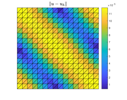
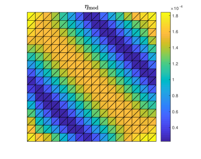
(a) $k=1,k^{\prime}=2$

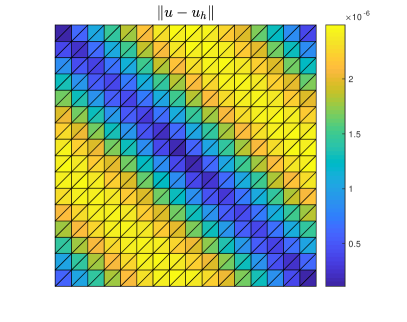
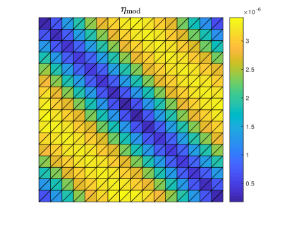
(b) $k=2,k^{\prime}=3$

Figure 1: Distribution of the errors $\|u-u_{h}\|_{K}$ (left) and of the local error estimators $\eta_{\mathrm{mod},K}$ (right) for the dG method (3.3) with $512$ elements; smooth solution (9.9), $\bm{b}=(1,1)^{\mathrm{t}}$, and different polynomial degrees $k$

9.5.2 Discontinuous solution

In this last example, we consider a discontinuous exact solution. For the velocity field $\bm{b}=(1,1)^{\mathrm{t}}$, we set

$$u(x,y)=\begin{cases}0,&x<y,\\ \sin(\pi x)\sin(\pi y),&x>y,\end{cases}$$ (9.10)

and prescribe accordingly the right-hand side $f$. The triangulation is set to be aligned with this discontinuity; hence, the reconstruction $s_{h}$ is continuous everywhere but not at the discontinuity line of the exact solution. The results are presented in Table 7 for different polynomial degrees $k$. They show the robustness with respect to the polynomial degree of approximation. In Figure 2, the distributions of the error and of the error estimators $\eta_{\mathrm{mod},K}$ are presented, again showing a very similar behavior.

Table 7: Convergence of the error $\|u-u_{h}\|$, the error estimators $\eta_{\mathrm{mod}}$, $\eta_{\mathrm{NC}}$, and $\eta_{\mathrm{R}}$, and the effectivity indices $I_{\mathrm{eff}}$ for the dG method (3.3); discontinuous solution (9.10), $\bm{b}=(1,1)^{\mathrm{t}}$, and different polynomial degrees $k$

$k=1,k^{\prime}=2$
# Elements	$\#$ DOF$(u_{h})$	$\eta_{\mathrm{NC}}$	$\eta_{\mathrm{R}}$	$\|u-u_{h}\|$	$\eta_{\mathrm{mod}}$	$I_{\mathrm{eff}}$
8	24	6.622e-02	1.473e-01	7.758e-02	1.538e-01	1.98
32	96	1.827e-02	2.939e-02	2.095e-02	3.445e-02	1.64
128	384	4.798e-03	6.127e-03	5.341e-03	7.780e-03	1.45
512	1536	1.221e-03	1.402e-03	1.341e-03	1.860e-03	1.38
2048	6144	3.074e-04	3.375e-04	3.358e-04	4.565e-04	1.36
8192	24576	7.705e-05	8.295e-05	8.399e-05	1.132e-04	1.35
$k=2,k^{\prime}=3$
# Elements	$\#$ DOF$(u_{h})$	$\eta_{\mathrm{NC}}$	$\eta_{\mathrm{R}}$	$\|u-u_{h}\|$	$\eta_{\mathrm{mod}}$	$I_{\mathrm{eff}}$
8	48	1.626e-02	7.463e-02	1.330e-02	3.680e-02	2.76
32	192	2.227e-03	5.102e-03	1.751e-03	3.105e-03	1.77
128	768	2.850e-04	3.544e-04	2.217e-04	3.454e-04	1.56
512	3072	3.583e-05	2.847e-05	2.778e-05	4.181e-05	1.50
2048	12288	4.485e-06	2.849e-06	3.489e-06	5.184e-06	1.48
8192	49152	5.610e-07	3.410e-07	4.433e-07	6.525e-07	1.47

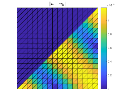
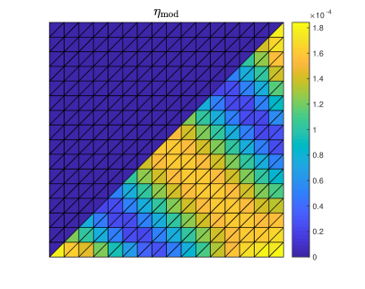
(a) $k=1,k^{\prime}=2$

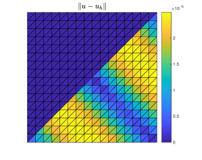
(b) $k=2,k^{\prime}=3$

Figure 2: Distribution of the errors $\|u-u_{h}\|_{K}$ (left) and of the local error estimators $\eta_{\mathrm{mod},K}$ (right) for the dG method (3.3) with $512$ elements; discontinuous solution (9.10), $\bm{b}=(1,1)^{\mathrm{t}}$, and different polynomial degrees $k$

10 Conclusions

In this work, we proposed a local reconstruction for numerical approximations of the one-dimensional linear advection equation, easily and independently obtained on each vertex patch. The reconstruction is proved to be well-posed and leads to a guaranteed upper bound of the $L_{2}$-norm error between the actual solution $u$ and the approximation $u_{h}$. This error estimator is also proved to be locally efficient and robust with respect to both the advective field and the approximation polynomial degree. These results hold in a unified framework that only requires the residual of $u_{h}$ to satisfy an orthogonality condition with respect to the hat basis functions. Numerical illustrations support the theory and additionally suggest asymptotic exactness. Motivated by these results, a heuristic extension to any space dimension is presented, with numerical experiments in 2D being in line with those in 1D.

References

- [1] O. Axelsson, J. Karátson, and B. Kovács, Robust preconditioning estimates for convection-dominated elliptic problems via a streamline Poincaré-Friedrichs inequality, SIAM J. Numer. Anal., 52 (2014), pp. 2957–2976.
- [2] B. Ayuso and L. D. Marini, Discontinuous Galerkin methods for advection-diffusion-reaction problems, SIAM J. Numer. Anal., 47 (2009), pp. 1391–1420.
- [3] P. Azérad and J. Pousin, Inégalité de Poincaré courbe pour le traitement variationnel de l’équation de transport, C. R. Acad. Sci. Paris Sér. I Math., 322 (1996), pp. 721–727.
- [4] R. Becker, D. Capatina, and R. Luce, Reconstruction-based a posteriori error estimators for the transport equation, in Numerical mathematics and advanced applications 2011, Springer, Heidelberg, 2013, pp. 13–21.
- [5] K. S. Bey and J. T. Oden, -version discontinuous Galerkin methods for hyperbolic conservation laws, Comput. Methods Appl. Mech. Engrg., 133 (1996), pp. 259–286.
- [6] J. Blechta, J. Málek, and M. Vohralík, Localization of the norm for local a posteriori efficiency, IMA J. Numer. Anal., (2019). DOI 10.1093/imanum/drz002.
- [7] D. Braess, V. Pillwein, and J. Schöberl, Equilibrated residual error estimates are -robust, Comput. Methods Appl. Mech. Engrg., 198 (2009), pp. 1189–1197.
- [8] P. Cantin, Well-posedness of the scalar and the vector advection-reaction problems in Banach graph spaces, C. R. Math. Acad. Sci. Paris, 355 (2017), pp. 892–902.
- [9] P. Cantin and A. Ern, An edge-based scheme on polyhedral meshes for vector advection-reaction equations, ESAIM Math. Model. Numer. Anal., 51 (2017), pp. 1561–1581.
- [10] C. Carstensen and S. A. Funken, Fully reliable localized error control in the FEM, SIAM J. Sci. Comput., 21 (1999), pp. 1465–1484.
- [11] W. Dahmen, C. Huang, C. Schwab, and G. Welper, Adaptive Petrov-Galerkin methods for first order transport equations, SIAM J. Numer. Anal., 50 (2012), pp. 2420–2445.
- [12] W. Dahmen and R. Stevenson, Adaptive strategies for transport equations, arXiv preprint arXiv:1809.02055, (2019).
- [13] A. Devinatz, R. Ellis, and A. Friedman, The asymptotic behavior of the first real eigenvalue of second order elliptic operators with a small parameter in the highest derivatives. II, Indiana Univ. Math. J., 23 (1973–1974), pp. 991–1011.
- [14] A. Ern and J.-L. Guermond, Discontinuous Galerkin methods for Friedrichs’ systems. I. General theory, SIAM J. Numer. Anal., 44 (2006), pp. 753–778.
- [15] A. Ern, A. F. Stephansen, and M. Vohralík, Guaranteed and robust discontinuous Galerkin a posteriori error estimates for convection-diffusion-reaction problems, J. Comput. Appl. Math., 234 (2010), pp. 114–130.
- [16] A. Ern and M. Vohralík, Polynomial-degree-robust a posteriori estimates in a unified setting for conforming, nonconforming, discontinuous Galerkin, and mixed discretizations, SIAM J. Numer. Anal., 53 (2015), pp. 1058–1081.
- [17] K. O. Friedrichs, Symmetric positive linear differential equations, Comm. Pure Appl. Math., 11 (1958), pp. 333–418.
- [18] E. H. Georgoulis, E. Hall, and C. Makridakis, Error control for discontinuous Galerkin methods for first order hyperbolic problems, in Recent developments in discontinuous Galerkin finite element methods for partial differential equations, vol. 157 of IMA Vol. Math. Appl., Springer, Cham, 2014, pp. 195–207.
- [19] , An a posteriori error bound for discontinuous Galerkin approximations of convection-diffusion problems, IMA J. Numer. Anal., 39 (2019), pp. 34–60.
- [20] F. Hecht, New development in FreeFEM++, J. Numer. Math., 20 (2012), pp. 251–265.
- [21] P. Houston, J. A. Mackenzie, E. Süli, and G. Warnecke, A posteriori error analysis for numerical approximations of Friedrichs systems, Numer. Math., 82 (1999), pp. 433–470.
- [22] P. D. Lax and R. S. Phillips, Local boundary conditions for dissipative symmetric linear differential operators, Comm. Pure Appl. Math., 13 (1960), pp. 427–455.
- [23] C. Makridakis and R. H. Nochetto, A posteriori error analysis for higher order dissipative methods for evolution problems, Numer. Math., 104 (2006), pp. 489–514.
- [24] I. Muga, M. J. Tyler, and K. van der Zee, The discrete-dual minimal-residual method (DDMRes) for weak advection-reaction problems in Banach spaces, arXiv preprint arXiv:1808.04542, (2018).
- [25] G. Sangalli, Analysis of the advection-diffusion operator using fractional order norms, Numer. Math., 97 (2004), pp. 779–796.
- [26] , A uniform analysis of nonsymmetric and coercive linear operators, SIAM J. Math. Anal., 36 (2005), pp. 2033–2048.
- [27] , Robust a-posteriori estimator for advection-diffusion-reaction problems, Math. Comp., 77 (2008), pp. 41–70.
- [28] D. Schötzau and L. Zhu, A robust a-posteriori error estimator for discontinuous Galerkin methods for convection-diffusion equations, Appl. Numer. Math., 59 (2009), pp. 2236–2255.
- [29] E. Süli, A posteriori error analysis and adaptivity for finite element approximations of hyperbolic problems, in An introduction to recent developments in theory and numerics for conservation laws (Freiburg/Littenweiler, 1997), vol. 5 of Lect. Notes Comput. Sci. Eng., Springer, Berlin, 1999, pp. 123–194.
- [30] Z. Tang, https://who.rocq.inria.fr/Zuqi.Tang/freefem++.html, 2015.
- [31] D. S. Tartakoff, Regularity of solutions to boundary value problems for first order systems, Indiana Univ. Math. J., 21 (1972), pp. 1113–1129.
- [32] R. Verfürth, Robust a posteriori error estimates for stationary convection-diffusion equations, SIAM J. Numer. Anal., 43 (2005), pp. 1766–1782.
- [33] R. Verfürth, A posteriori error estimation techniques for finite element methods, Numerical Mathematics and Scientific Computation, Oxford University Press, Oxford, 2013.