Abstract

We develop an approach where the quantum system states and quantum observables are described as in classical statistical mechanics – the states are identified with probability distributions and observables, with random variables. An example of the spin-1/2 state is considered. We show that the triada of Malevich’s squares can be used to illustrate the qubit state. We formulate the superposition principle of quantum states in terms of probabilities determining the quantum states. New formulas for nonlinear addition rules of probabilities providing the probabilities associated with the interference of quantum states are obtained. The evolution equation for quantum states is given in the form of a kinetic equation for the probability distribution identified with the state.

Keywords: probability distribution, qubit, density matrix, foundation of quantum mechanics, hidden variables.

1 Introduction

The aim of our work is to demonstrate that in usual quantum mechanics the notion of quantum system state can be formulated analogously to the notion of classical system state in classical statistical mechanics, namely, the quantum state can be identified with the probability distribution. The classical system state, e.g., a state of the classical particle, is described by the particle position $q$ and the particle velocity $\dot{q}$ [1] or the particle momentum $p=m\,\dot{q}$, where $m$ is the particle mass.

If there are thermal fluctuations of the particle position and momentum, the classical particle state is identified with the probability density $f(q,p)$, which is a nonnegative function on the phase-space plane with the normalization condition $\displaystyle{\int}f(q,p)\,dq\,dp=1$. The other example of classical system is a classical coin employed in the coin tossing game.

If the coin is a nonideal one, its states corresponding to the position “up” or “down” are described by the probability distributions associated with the probability vectors $\vec{p}=(p_{1},p_{2})$ with the nonnegative components $p_{1}$ and $p_{2}$ satisfying the normalization condition $p_{1}+p_{2}=1$. Here, $p_{1}$ is the probability to have the coin position “up” and $p_{2}$ is the probability to have the coin position “down” in the coin tossing game.

For an ideal coin, the probabilities of the coin position “up” and “down” are equal, i.e., $p_{1}=p_{2}=1/2$. The positions “up” and “down” are random positions. We can identify the label “up” with the number 1 and the position label “down” with the number 2. This means that we can consider the coin probability distribution $p(j)$ as a function of random positions labeled by the integers (random positions) $j=1,2$.

In the coin tossing game, we can consider the other random variables given by functions $f(j)$, where $f(1)$ is identified with the gain in the game, and $f(2)$ is identified with the loss in the game. The classical statistics in the coin tossing game is associated with random variable means $\langle f\rangle=p_{1}f(1)+p_{2}f(2)$ and other highest moments $\langle f^{n}\rangle=p_{1}f^{n}(1)+p_{2}f^{n}(2);\,n=2,3\ldots$

The coin state characteristics are given, e.g., by the Shannon entropy $H=-p_{1}\ln p_{1}-p_{2}\ln p_{2}$ [2, 3, 4, 5, 6, 7]. There are other kinds of entropies, e.g., Tsallis entropy [8] and Rényi entropy [9]. In this paper, we show that the same probability distributions of classical coin positions determine these entropies for quantum states of qubits.

If there are several coins, it is obvious that the states of these coins are described by a set of the probability distributions $p_{j}^{(n)}$, where $j=1,2$ and $n=1,2,\ldots N$. The label $n$ corresponds to the $n$th coin probability distribution. If there is no correlations among the coins, the probabilities $p_{1}^{(n)}$ and $p_{2}^{(n)}$ satisfy the only constraints $0\leq p_{1}^{(n)},\,p_{2}^{(n)}\leq 1$ and $p_{1}^{(n)}+p_{2}^{(n)}=1$.

In the case of a dependence of coin positions, extra relations can exist for numbers $p_{1}^{(n)}$ and $p_{2}^{(n)}$. For example, if two coins are completely identical, we have $p_{j}^{(1)}=p_{j}^{(2)}$; this means that one has the possibility to consider the probability distributions for two coins, where the distribution for second coin is completely determined by the probability distribution for the first coin, being simply the same distribution.

In quantum mechanics, Schrödinger [10] introduced the notion of the particle state (pure state), identifying it with the complex wave function $\psi(q)=|\psi(q)|\exp[i\phi(q)]$. The modulus of the wave function has the intuitively clear physical meaning of the probability density $P_{\psi}(q)=|\psi(q)|^{2}$, but the phase of the complex wave function $\phi(q)$ does not have an analogous probabilistic interpretation.

The influence of thermal fluctuations was taken into account by considering mixed states of the particle. Landau [11] and von Neumann [12] introduced the notion of mixed states identifying the particle state with complex Hermitian density matrix $\rho(q,q^{\prime})$, which is a function of two variables with the property $\rho(q,q^{\prime})=\rho^{\ast}(q^{\prime},q).$ For normalized states $\displaystyle{\int}\rho(q,q)\,dq=1$ and for pure states with wave function $\psi(q)$, the density matrix is expressed in terms of the wave function $\rho_{\psi}(q,q^{\prime})=\psi(q)\psi^{\ast}(q^{\prime})$. This picture was generalized by Dirac, and the pure states were identified with the state vectors $|\psi\rangle$, and the mixed states were identified with the density operators $\hat{\rho}$, where the vectors live in the Hilbert space, and operators $\hat{\rho}$ act in the Hilbert space [13].

One can see that the described notion of quantum system states is drastically different from the considered notion of states in classical statistics. In view of this, from the early days of quantum mechanics there were attempts to find the formulation of quantum mechanics with the possibility to associate the states with other functions, which are similar to functions used in classical statistics. The first attempt was made by Wigner [14], who introduced the Wigner function $W(p,q)$, which is similar to the classical probability distribution $f(q,p)$ but this function is not the probability density since it can take negative values.

Later Husimi [15] and Kano [16] introduced the function $Q(q,p)$, which has only nonnegative values, but its continuous variables $q$ and $p$ are not physical observables (position and momentum), since the uncertainty relations [17, 18, 19] prohibit one from measuring simultaneously the position and momentum. This means that a joint probability distribution of two random continuous position and momentum does not exist. In view of this fact, the Wigner and Husimi–Kano functions are called quasidistributions.

Other kinds of quasidistributions $P(q,p)$ were introduced by Glauber [20] and Sudarshan [21] and by Blokhintsev [22, 23]. All these quasidistributions are related by different integral transforms with the density matrix $\rho(q,q^{\prime})$. They are different representations of the density operator $\hat{\rho}$ determining the state of the particle. In [24], the notion of the quantum particle state was introduced, which identifies it with the fair probability density $w(X,\mu,\nu)$ of a random variable $X$ and parameters $\mu$ and $\nu$, called a symplectic tomogram, which is a nonnegative function satisfying the normalization condition $\displaystyle{\int}w(X,\mu,\nu)\,dX=1$.

A symplectic tomogram is a generalization of the optical tomogram $w(X,\theta)$ [25, 26] used in experiments [27] as a technical instrument to measure the photon state identified with the Wigner function. The idea of [24, 28] was to suggest the identification of the quantum-particle-state notion with standard probability density. It was shown in [29] that the notion of symplectic tomogram $w(X,\mu,\nu)$ and optical tomogram $w(X,\theta)$ can be also introduced in classical statistics, where these probability densities are expressed in terms of the probability density $f(q,p)$ by means of the invertible integral Radon transform [30].

In classical statistics, this transform maps the probability density $f(q,p)$ onto the tomographic probability density [31]. Interestingly, in quantum mechanics exactly the same invertible transform maps the Wigner quasidistribution $W(q,p)$, which can take negative values, onto a fair nonnegative tomographic probability density. Reviews of this approach are given in [32, 33, 34, 35]. Examples of using the tomographic probability distributions for oscillator systems were presented in [36, 37, 38].

It turned out that the probability distribution determining the spin states (qudit states, $N$-level atom states) can be also introduced [39, 40, 41, 42, 43, 44]. There exist the bijective maps of density matrices of spin states onto standard probability distributions both of tomographic probability type [45, 46, 47, 48] and the coin tossing game type [49, 50, 51, 52, 53, 54, 55, 56, 57, 58]. In the case of qudit states, the quantum observables (Hermitian matrices) can be mapped bijectively onto sets of classical-like dichotomic variables [49, 50, 51, 52, 53, 54].

The aim of the paper is to present a review of the suggested probability representation of quantum system states, including the superposition principle of the states expressed in terms of the new nonlinear addition rule of the probabilities [51] and illustration of the qubit states in quantum suprematism picture [53, 54], where the Bloch sphere parameters of the states are bijectively mapped onto the triada of Malevich’s squares (red, black, and white) associated with triangle geometry of these states [49, 50, 51, 52, 53, 54, 56, 57].

This paper is organized as follows.

In Sec. 2, the elements of complex matrix are expressed in terms of the probabilities. In Sec. 3, the bijective map for classical random variables used in the coin tossing game and Hermitian operators acting in the Hilbert space are constructed. In Sec. 4, the superposition principle in the probability representation is reviewed. In Sec. 5, the unitary evolution of the density matrix is expressed in terms of probability distribution transforms. In Sec. 6, the notion of quantum suprematism is discussed, and the main results of this work are pointed out in Sec. 7.

2 Matrices as Probability Distribution

We discuss the map of the generic matrices onto the probability distributions. Such map seems to have not been considered in the literature. In [59], the matrices $A$ were bijectively mapped onto vectors $|A\rangle$, using the rule illustrated by the example of 2$\times$2 matrices

$$A=\left(\begin{array}[]{cc}A_{11}&A_{22}\\ A_{21}&A_{22}\end{array}\right)\leavevmode\nobreak\ \leftrightarrow\leavevmode\nobreak\ |A\rangle=\left(\begin{array}[]{c}A_{11}\\ A_{12}\\ A_{21}\\ A_{22}\end{array}\right).$$ (1)

Thus, the matrix elements in the rows of the matrix $A$ construct the column of the vector $|A\rangle$. The 4$\times$4 matrix $A$$\times$$A^{\ast}$ is bijectively mapped onto the 16-dimensional vector $|A^{\prime}\rangle$ with components $A_{1}=|A_{11}|^{2},$ $A_{2}=A_{11}A^{\ast}_{12}$, $A_{3}=A_{12}A^{\ast}_{11}$, $A_{4}=|A_{12}|^{2},$ $A_{5}=A_{11}A_{21}^{\ast},$ $A_{6}=A_{11}A_{22}^{\ast}$, $A_{7}=A_{12}A_{21}^{\ast}$, $A_{8}=A_{12}A_{22}^{\ast}$, $A_{9}=A_{21}A_{11}^{\ast},$ $A_{10}=A_{21}A_{12}^{\ast}$, $A_{11}=A_{22}A_{11}^{\ast}$, $A_{12}=A_{22}A_{12}^{\ast}$, $A_{13}=|A_{21}|^{2}$, $A_{14}=A_{21}A_{22}^{\ast}$, $A_{15}=A_{22}A_{21}^{\ast}$, and $A_{16}=|A_{22}|^{2}.$

The matrix $|A\rangle\langle A|$ is mapped onto the other vector with 16 components, namely, the vector $|\tilde{A}\rangle$. Its components are $\tilde{A}_{1}=|A_{11}|^{2},$ $\tilde{A}_{2}=A_{11}A^{\ast}_{12}$, $\tilde{A}_{3}=A_{11}A^{\ast}_{21}$, $\tilde{A}_{4}=A_{11}A_{22}^{\ast},$ $\tilde{A}_{5}=A_{12}A_{11}^{\ast},$ $\tilde{A}_{6}=|A_{12}|^{2}t$, $\tilde{A}_{7}=A_{12}A_{21}^{\ast}$, $\tilde{A}_{8}=A_{12}A_{22}^{\ast}$, $\tilde{A}_{9}=A_{21}A_{11}^{\ast},$ $\tilde{A}_{10}=A_{21}A_{12}^{\ast}$, $\tilde{A}_{11}=|A_{21}|^{2}$, $\tilde{A}_{12}=A_{21}A_{22}^{\ast}$, $\tilde{A}_{13}=A_{22}A_{11}^{\ast}$, $\tilde{A}_{14}=A_{22}A_{12}^{\ast}$, $\tilde{A}_{15}=A_{22}A_{21}^{\ast}$, and $\tilde{A}_{16}=|A_{22}|^{2}.$

The vectors $|A^{\prime}\rangle$ and $|\tilde{A}\rangle$ are connected by the unitary transform

$$|A^{\prime}\rangle=T|\tilde{A}\rangle,$$ (2)

where the 16$\times$16 matrix $T$ has the block form $T_{ik}$ with unity and zero 2$\times$2 blocks $(i,k=1,2,\ldots,8)$. The nonzero blocks are $T_{11}=T_{13}=T_{31}=T_{44}=T_{55}=T_{67}=T_{76}=T_{88}=1_{2}$. The matrix

$$\rho=\frac{|\tilde{A}\rangle\langle\tilde{A}|}{\langle\tilde{A}|\tilde{A}\rangle}$$

is the Hermitian matrix, and its trace is equal to unity. The eigenvalues of this matrix are equal either to zero or unity, i.e., $\rho^{2}=\rho$ and $\mbox{Tr}\rho^{2}=\mbox{Tr}\rho=1$.

As it was conjectured in [53, 54, 55, 56, 57], an arbitrary 4$\times$4 matrix $\rho$ with such properties (it can be interpreted as the density matrix of the pure state of spin-3/2 system or of two-qubit systems) has the probability parametrization, i.e., the matrix is

$$\rho=\left(\begin{array}[]{cccc}\rho_{11}&\rho_{12}&\rho_{13}&\rho_{14}\\ \rho_{21}&\rho_{22}&\rho_{23}&\rho_{24}\\ \rho_{31}&\rho_{32}&\rho_{33}&\rho_{34}\\ \rho_{41}&\rho_{42}&\rho_{43}&\rho_{44}\end{array}\right),$$ (3)

where nonnegative numbers

$$\rho_{22}=1-p_{3}^{(22)},\quad\rho_{33}=1-p_{3}^{(33)},\quad\rho_{44}=1-p_{3}^{(44)},\quad\rho_{11}=\rho_{3}^{(22)}+\rho_{3}^{(33)}+p_{3}^{(44)}-2$$ (4)

provide the diagonal matrix elements of the matrix $\rho$ in terms of probabilities $0\geq p_{3}^{(22)}\geq 1$, $0\geq p_{3}^{(33)}\geq 1$, and $0\geq p_{3}^{(44)}\geq 1$ associated with three probability distributions $(p_{3}^{(22)},1-p_{3}^{(22)})$, $(p_{3}^{(33)},1-p_{3}^{(33)})$, and $(p_{3}^{(44)},1-p_{3}^{(44)})$ describing the tossing coin game for three coins labeled by indices $(22)$, $(33)$, and $(44)$. The nondiagonal elements $\rho_{jk},\,j>k$ of the matrix $\rho$ read

$$\rho_{jk}=p_{1}^{(jk)}-(1/2)+i(p_{2}^{(jk)}-1/2),\qquad j,k=2,3,4,\quad j>k,$$ (5)

where the nonnegative numbers $0\leq p_{1}^{(jk)}\leq 1$ and $0\leq p_{2}^{(jk)}\leq 1$ are associated with the probability distributions $(p_{1}^{(jk)},1-p_{1}^{(jk)})$ and $(p_{2}^{(jk)},1-p_{2}^{(jk)})$ describing the tossing coin gains for 12 coins labeled by the indices $(jk)$.

The probabilities satisfy the inequalities of nonnegativity of the matrix $\rho\geq 0$. If the matrix $A$ satisfies the condition $\mbox{Tr}(A^{\dagger}A)=1$, its matrix elements can be connected with the probabilities $p_{1,2,3}^{(jk)}$; $j,k=1,2,3,4$ as follows:

$$|A_{11}|^{2}=p_{3}^{(22)}+p_{3}^{(33)}+p_{3}^{(44)}-2,$$

$$A_{11}A_{12}^{\ast}=p_{1}^{(12)}-(1/2)-i(p_{2}^{(12)}-1/2)=x,$$

$$A_{11}A_{21}^{\ast}=p_{1}^{(13)}-(1/2)-i(p_{2}^{(13)}-1/2)=y,$$

$$A_{11}A_{22}^{\ast}=p_{1}^{(14)}-(1/2)-i(p_{2}^{(14)}-1/2)=z,$$

$$|A_{12}|^{2}=1-p_{3}^{(22)},\quad A_{12}A_{21}^{\ast}=p_{1}^{(23)}-(1/2)-i(p_{2}^{(23)}-1/2)=m,$$

(6)

$$A_{12}A_{22}^{\ast}=p_{1}^{(24)}-(1/2)-i(p_{2}^{(24)}-1/2)=n,\quad|A_{21}|^{2}=1-p_{3}^{(33)},$$

$$A_{21}A_{22}^{\ast}=p_{1}^{(34)}-(1/2)-i(p_{2}^{(34)}-1/2)=t,\quad|A_{22}|^{2}=1-p_{3}^{(44)},$$

$$|A_{11}|^{2}+|A_{21}|^{2}+|A_{12}|^{2}+|A_{22}|^{2}=1.$$

Relations (6) provide the possibility to express the complex matrix elements $A_{11},\,A_{12},\,A_{21},\,A_{22}$ given by seven parameters of the matrix $A_{jk}$; $j,k=1,2$ in terms of the above probabilities $p_{1,2}^{(jk)}$, where $j,k=1,2,3,4$, and $p_{3}^{(jj)}$, where $j=2,3,4.$

We demonstrated that for the matrix $A$ one can introduce the probability representation. An analogous construction can be introduced for $N$$\times$$N$ matrix $A$, where $N=3,4,\ldots$

3 Qubit States as the Quantization of Classical Coin Probability Distributions

As we demonstrated in the previous section, the matrix elements of an arbitrary matrix $A$ can be related to some probability distributions. We use this observation to suggest the following quantization procedure of classical statistics. We construct from classical probability distributions, describing the coin states, the density matrices and state vectors in a Hilbert space. This means that we map the probability distributions (simplexes) onto density operators acting in the Hilbert space. Also we map the classical random variables, used in the coin tossing game, onto Hermitian matrices, i.e., Hermitian operators acting in the Hilbert space. The map constructed is a bijective map.

After the map was constructed, we obtain all the relations known in quantum mechanics rewritten as the relations for classical-like random variables and standard probability distributions. We demonstrate this procedure on the example of spin-1/2 (qubit, two-level atom) state and spin observables.

Let us start with tossing three nonideal classical coins. The states of these three coins are identified with three probability distributions with probabilities $0\leq p_{1},p_{2},p_{3}\leq 1$, i.e., $(p_{1},1-p_{1})$, $(p_{2},1-p_{2})$, and $(p_{3},1-p_{3})$. The probabilities $p_{1}$, $p_{2}$, and $p_{3}$ are the probabilities in the game to have for each coin the position “up.”

As we discussed in the introduction, the dichotomic random variables $f^{(n)}(j)$; $j=1,2;\,n=1,2,3$ associated with these three coins can be denoted as $f^{(1)}(1)=x;\,f^{(1)}(2)=-x,\,f^{(2)}(1)=y;\,f^{(2)}(2)=-y$, and $f^{(3)}(1)=z_{1};\,f^{(3)}(2)=z_{2}$, where $x,y,z_{1}$, and $z_{2}$ are real numbers. The statistics of the coin tossing game provides mean values of random variables, such as

$$\langle f^{(1)}\rangle=xp_{1}-x(1-p_{1}),\quad\langle f^{(2)}\rangle=yp_{2}-y(1-p_{2}),\quad\langle f^{(3)}\rangle=p_{3}z_{1}+(1-p_{3})z_{2}.$$ (7)

The highest moments of the classical random variables are given by standard formulas of the probability theory ($k=2,3,\ldots$) as follows:

$$\langle f^{(1)k}\rangle=x^{k}p_{1}+(-x)^{k}(1-p_{1}),\quad\langle f^{(2)k}\rangle=y^{k}p_{2}+(-y)^{k}(1-p_{2}),\quad\langle f^{(3)k}\rangle=p_{3}z_{1}^{k}+(1-p_{3})z_{2}^{k}.$$ (8)

Let us organize the numbers $p_{1}$, $p_{2}$, and $p_{3}$ in table form given as the 2$\times$2 matrix

$$\rho=\left(\begin{array}[]{cc}p_{3}&p_{1}-1/2-i(p_{2}-1/2)\\ p_{1}-1/2+i(p_{2}-1/2)&1-p_{3}\end{array}\right).$$ (9)

The states of classical three coins can be associated with matrix elements of the Hermitian trace-one matrix $\rho$.

Now we introduce the quantization procedure; namely, we impose the condition for this Hermitian matrix $\rho$ to have only nonnegative eigenvalues. This means that $\mbox{det}\rho\geq 0$ or the probabilities $p_{1}$, $p_{2}$, and $p_{3}$ satisfy the condition

$$(p_{1}-1/2)^{2}+(p_{2}-1/2)^{2}+(p_{3}-1/2)^{2}\leq 1/4.$$ (10)

Comparing matrix (9) with density matrices of spin-1/2 states, we see that matrix (9) simulates all the possible quantum states of this system. For the case $\rho^{2}=\rho$, we obtain the condition for pure spin-1/2 states

$$(p_{1}-1/2)^{2}+(p_{2}-1/2)^{2}+(p_{3}-1/2)^{2}=1/4.$$ (11)

In this case, we can construct the vector $|\psi\rangle$ in the Hilbert space, which provides the matrix elements of the matrix $\rho$. One can check that the vector $|\psi\rangle$ in Dirac notation reads

$$|\psi\rangle=\left(\begin{array}[]{c}\sqrt{p_{3}}\\[5.69054pt] \frac{p_{1}-(1/2)+i(p_{2}-1/2)}{\sqrt{p_{3}}}\end{array}\right).$$ (12)

In fact, $|\psi\rangle\langle\psi|=\rho_{\psi}$. We constructed this vector by introducing a triple of normalized vectors of the basis in the linear space ${\cal H}$ (the Hilbert space) of the form

$$|1\rangle_{z}=\left(\begin{array}[]{c}1\\ 0\end{array}\right),\quad|2\rangle_{z}=\left(\begin{array}[]{c}0\\ 1\end{array}\right),\quad|1\rangle_{x}=\frac{1}{\sqrt{2}}\left(\begin{array}[]{c}1\\ 1\end{array}\right),$$ (19)

(20)

$$|2\rangle_{x}=\frac{1}{\sqrt{2}}\left(\begin{array}[]{c}1\\ -1\end{array}\right),\quad|1\rangle_{y}=\frac{1}{\sqrt{2}}\left(\begin{array}[]{c}1\\ i\end{array}\right),\quad|2\rangle_{y}=\frac{1}{\sqrt{2}}\left(\begin{array}[]{c}1\\ -i\end{array}\right).$$ (27)

We introduced these special basis vectors (not yet considered in the literature of the usual probability theory), since they provide the matrices

$$\rho_{x}^{(1/2)}=(|1\rangle_{x}\,{}_{x}\langle 1|)=\frac{1}{2}\left(\begin{array}[]{cc}1&1\\ 1&1\end{array}\right),\qquad\rho_{x}^{(-1/2)}=(|2\rangle_{x}\,{}_{x}\langle 2|)=\frac{1}{2}\left(\begin{array}[]{cc}1&-1\\ -1&1\end{array}\right),$$ (32)

$$\rho_{y}^{(1/2)}=(|1\rangle_{y}\,{}_{y}\langle 1|)=\frac{1}{2}\left(\begin{array}[]{cc}1&-i\\ i&1\end{array}\right),\qquad\rho_{y}^{(-1/2)}=(|2\rangle_{y}\,{}_{y}\langle 2|)=\frac{1}{2}\left(\begin{array}[]{cc}1&i\\ -i&1\end{array}\right),$$ (37)

$$\rho_{z}^{(1/2)}=\frac{1}{2}|1\rangle_{z}\,{}_{z}\langle 1|=\frac{1}{2}\left(\begin{array}[]{cc}1&0\\ 0&0\end{array}\right),\qquad\rho_{z}^{(-1/2)}=\frac{1}{2}|2\rangle_{z}\,{}_{z}\langle 2|=\frac{1}{2}\left(\begin{array}[]{cc}0&0\\ 0&1\end{array}\right).$$ (42)

The Hermitian matrices (37) are related to the classical random variables $x,\,y,\,z_{1}$, and $z_{2}$. In fact, one can organized these random variables in the form of Hermitian matrix

$$H=\left(\begin{array}[]{cc}z_{1}&x-iy\\ x+iy&z_{2}\end{array}\right).$$ (43)

These matrices can be expressed in terms of the identity matrix 1 and Pauli matrices

$$\sigma_{x}=\left(\begin{array}[]{cc}0&1\\ 1&0\end{array}\right),\qquad\sigma_{y}=\left(\begin{array}[]{cc}0&-i\\ i&0\end{array}\right),\qquad\sigma_{z}=\left(\begin{array}[]{cc}1&0\\ 0&-1\end{array}\right).$$ (44)

One has

$$H=\frac{1}{2}\left[(z_{1}+z_{2}){\bf 1}+(z_{1}-z_{2})\sigma_{z}+x\sigma_{x}+y\sigma_{y}\right].$$ (45)

Expressions (37)–(45) show that an arbitrary quantum spin-1/2 observable presented by the Hermitian matrix $H$ can be simulated by three classical dichotomic random variables taking values $(x,-x)$, $(y,-y)$, and $(z_{1},z_{2})$. For example, the spin-1/2 projection $s_{x}=\sigma_{x}/2,$ $s_{y}=\sigma_{y}/2$, and $s_{z}=\sigma_{z}/2$ are simulated by classical random variables; namely, for the $s_{x}$ observable, the random variables are $z_{1}=z_{2}=0$, $x=1/2$, $-x=-1/2$, and $y=0$; for the $s_{y}$ observable, $z_{1}=z_{2}=0$, $x=0$, $y=1/2$, and $-y=-1/2$; for the $s_{z}$ observable, $x=0$, $y=0$, $z_{1}=1/2$, and $z_{2}=-1/2$. Thus, for the coin tossing game, the conditions associated with spin projections onto three perpendicular directions give observables corresponding to the three coins, and they are equivalent for the directions of axes $x,$ $y$, and $z$.

If we organize the classical random variables in the form of Hermitian matrices, the different observables do not commute. For spin projections, the quantum observables $s_{x}$, $s_{y}$, and $s_{z}$ provide the commutation relation

$$[s_{x},s_{y}]=(s_{x}s_{y}-s_{y}s_{x})=is_{z}.$$ (46)

As well as the condition (10), this relation means that our quantization procedure imposes correlations for classical coin states and observables. The quantization condition means also that, if we impose the formula for statistical properties of the quantum observable $H$ of standard form

$$\langle H^{k}\rangle=\mbox{Tr}(\rho H^{k}),\,k=1,2,\ldots,$$ (47)

the quantum statistics can be related to classical probabilities simulating the state $\rho$ and classical random dichotomic variables simulating the quantum observable $H$. For example, the mean value of $H$ is

$$\langle H\rangle=x(2p_{1}-1)+y(2p_{2}-1)+p_{3}(z_{1}-z_{2})+z_{2}.$$ (48)

The quantization procedure of classical random variables by means of writing the variables $x,$ $y$, $z_{1}$, and $z_{2}$ in the matrix form (15) means the imposing the condition that the eigenvalues of the matrix $H$ are the values that provide the results of the measurement of quantum observable (17) in the state with density matrix (9). Thus, the quantization procedure gives the possible values of quantum observable eigenvalues $H_{1}$ and $H_{2}$ expressed in terms of three classical random variables of the form

$$H_{1}=\frac{z_{1}+z_{2}}{2}+\sqrt{\frac{(z_{1}-z_{2})^{2}+x^{2}+y^{2}}{4}},\qquad H_{2}=\frac{z_{1}+z_{2}}{2}-\sqrt{\frac{(z_{1}-z_{2})^{2}+x^{2}+y^{2}}{4}}.$$ (49)

We also point out that the eigenvalues $\lambda_{1}$ and $\lambda_{2}$ of the density matrix $\rho$ (9) are the probabilities expressed in terms of the probabilities $p_{1}$, $p_{2}$, and $p_{3}$ as follows:

$$\lambda_{1}=\frac{1}{2}+\left\{\frac{1}{4}-\left[p_{3}(1-p_{3})-(p_{1}-1/2)^{2}-(p_{2}-1/2)^{2}\right]\right\}^{1/2},$$

(50)

$$\lambda_{2}=\frac{1}{2}-\left\{\frac{1}{4}-\left[p_{3}(1-p_{3})-(p_{1}-1/2)^{2}-(p_{2}-1/2)^{2}\right]\right\}^{1/2}.$$

The eigenvectors of the matrix $\rho$ read

$$|\rho_{1}\rangle=\left[1+\frac{\lambda_{1}-p_{3}}{(p_{1}-1/2)^{2}+(p_{2}-1/2)^{2}}\right]^{-1/2}\left(\begin{array}[]{c}1\\ \frac{\lambda_{1}-p_{3}}{(p_{1}-1/2)-i(p_{2}-1/2)}\end{array}\right),$$ (53)

(54)

$$|\rho_{2}\rangle=\left[1+\frac{\lambda_{2}-p_{3}}{(p_{1}-1/2)^{2}+(p_{2}-1/2)^{2}}\right]^{-1/2}\left(\begin{array}[]{c}1\\ \frac{\lambda_{2}-p_{3}}{(p_{1}-1/2)-i(p_{2}-1/2)}\end{array}\right).$$ (57)

The eigenvectors of the matrix $H$ determine the mean values of quantum observables $H$ in a given state with the density matrix (9). In fact, the unitary matrix $U$, such that

$$H=\left(\begin{array}[]{cc}u_{11}&u_{12}\\ u_{21}&u_{22}\end{array}\right)\left(\begin{array}[]{cc}H_{1}&0\\ 0&H_{2}\end{array}\right)\left(\begin{array}[]{cc}u^{\ast}_{11}&u^{\ast}_{12}\\ u^{\ast}_{21}&u^{\ast}_{22}\end{array}\right),$$ (64)

defines the bistochastic matrix

$$M=\left(\begin{array}[]{cc}|u_{11}|^{2}&|u_{12}|^{2}\\ |u_{21}|^{2}&|u_{22}|^{2}\end{array}\right),$$ (65)

where the probability

$$|u_{11}|^{2}=\left[1+\frac{|H_{1}-z_{1}|^{2}}{x^{2}+y^{2}}\right]^{-1/2}$$ (66)

relates the mean value $H_{11}$ of the observable $H$ with the eigenvalues (21) as follows:

$$H_{11}=|u_{11}|^{2}H_{1}+(1-|u_{11}|^{2})H_{2},$$ (67)

$$H_{22}=|u_{11}|^{2}H_{2}+(1-|u_{11}|^{2})H_{1},$$ (68)

Formulas (21), (22), and (66)–(68) provide the expressions of quantum eigenvalues and eigenvectors both for observables $H$ and density matrix $\rho$ in terms of classical coin probabilities $p_{1},p_{2}$, and $p_{3}$ and classical observables $x,y,z_{1}$, and $z_{2}$.

The von Neumann entropy $S=-\mbox{Tr}\rho\ln\rho$ of the quantum state with density matrix (9) is expressed in terms of classical coin probabilities $p_{1},p_{2}$, and $p_{3}$, in view of Eq. (50),

$$S=-\lambda_{1}\ln\lambda_{1}-\lambda_{2}\ln\lambda_{2}.$$ (69)

Also the Tsallis entropy of quantum states can be expressed in terms of classical probabilities as

$$S_{T}=\frac{\lambda_{1}^{q}+\lambda_{2}^{q}-1}{1-q},$$ (70)

where $\lambda_{1}$ and $\lambda_{2}$ depend on the coin position probabilities $p_{1},p_{2}$, and $p_{3}.$

In view of our approach, we can formulate a problem analogous to the one studied by Koopman [60] and von Neumann [61]. The initial idea was to formulate quantum mechanics using the formalism of classical statistics. The inverse problem considered in [60, 61] was to formulate classical statistical mechanics using the formalism of quantum mechanics like a Hilbert space and operators acting in the Hilbert space. Some examples of this approach are related to constructing the wave function of classical oscillator [62, 63, 64].

The problem that we are now considering is an analogous one. Namely, it is possible that the standard probability theory or the theory of simplexes is mapped onto the formalism of Hilbert spaces and operators acting in the Hilbert spaces. We see that in the usual probability theory the constructions induced by the relations available in quantum mechanics appear. These constructions seem not to have been considered in the literature connected with the probability theory like pseudostochastic matrices [65], transforming probability distributions with constraints related to the density-matrix properties. Such kinds of probability-theory problems can be solved using the solutions of quantum mechanics problems in the probability representation of quantum states and sequent employment of the map of discussed properties of states and observables onto probability distributions and random variables.

4 Superposition Principle in the Probability Representation

Since the pure qubit states are expressed in terms of probabilities, one can obtain the formulas for the superposition of states $|\psi_{1}\rangle$ and $|\psi_{2}\rangle$ in the form of addition of the probabilities. To obtain these formulas, we use the results [59] where the superposition of two pure states with density operators $\hat{\rho}_{1}=|\psi_{1}\rangle\langle\psi_{1}|$ and $\hat{\rho}_{2}=|\psi_{2}\rangle\langle\psi_{2}|$ was expressed as a nonlinear addition of the density operators giving the projector $\hat{\rho}_{\psi}$, which is

$$\hat{\rho}_{\psi}=\lambda_{1}\hat{\rho}_{1}+\lambda_{2}\hat{\rho}_{2}+\sqrt{\lambda_{1}\lambda_{2}}\,\frac{\hat{\rho}_{1}\hat{\rho}_{0}\hat{\rho}_{2}+\hat{\rho}_{2}\hat{\rho}_{0}\hat{\rho}_{1}}{\sqrt{\mbox{Tr}(\hat{\rho}_{1}\hat{\rho}_{0}\hat{\rho}_{2}\hat{\rho}_{0})}}.$$ (71)

Here, $0\leq\lambda_{1}$, $\lambda_{2}\leq 1$, and $\lambda_{1}+\lambda_{2}=1$ are the probabilities, and $\hat{\rho}_{1}$, $\hat{\rho}_{0}$, and $\hat{\rho}_{2}$ are given pure-state density operators written in the probability representation. Expressing the pure state density matrices $\rho_{\psi}$, $\rho_{1},$ ,$\rho_{2}$, and $\rho_{0}$ in terms of the probabilities, we derive the addition rule of probabilities [51, 66] corresponding to the quantum superposition principle. It can be given as follows.

For probabilities $p_{1},p_{2},p_{3}$,${\cal P}_{1}$, ${\cal P}_{2}$, ${\cal P}_{3}$,$\Pi_{1}$, $\Pi_{2}$, and $\Pi_{3}$, the probabilities corresponding to the density matrix $\rho_{\psi}$ are given by the expressions

$$P_{3} = ({1}/{{\cal T}})\left\{\Pi_{3}p_{3}+(1-\Pi_{3}){\cal P}_{3}+2\sqrt{p_{3}{\cal P}_{3}}\left(\Pi_{1}-1/2\right)\right\},$$ (72)

$$P_{1}-1/2 = ({1}/{{\cal T}})\Big{\{}\Pi_{3}(p_{1}-1/2)+({\cal P}_{1}-1/2)(1-\Pi_{3})$$ (73)

$$+\left[(\Pi_{1}-1/2)(p_{1}-1/2)+(\Pi_{2}-1/2)(p_{2}-1/2)\right]\sqrt{{{\cal P}_{3}}/{p_{3}}}$$

$$+\left.\left[(\Pi_{1}-1/2)({\cal P}_{1}-1/2)-(\Pi_{2}-1/2)({\cal P}_{2}-1/2)\right]\sqrt{{p_{3}}/{{\cal P}_{3}}}\right\},$$

$$P_{2}-1/2 = ({1}/{{\cal T}})\Big{\{}\left[(p_{2}-1/2)\Pi_{3}+({\cal P}_{2}-1/2)(1-\Pi_{3})\right]$$ (74)

$$+\sqrt{{{\cal P}_{3}}/{p_{3}}}\left[(\Pi_{1}-1/2)(p_{2}-1/2)-(\Pi_{2}-1/2)(p_{1}-1/2)\right]$$

$$+\left.\sqrt{{p_{3}}/{{\cal P}_{3}}}\left[(\Pi_{2}-1/2)({\cal P}_{1}-1/2)+(\Pi_{1}-1/2)({\cal P}_{2}-1/2)\right]\right\},$$

where the parameter ${\cal T}$ reads

$${\cal T} = 1+\frac{2}{\sqrt{p_{3}{\cal P}_{3}}}\left\{(\Pi_{1}-1/2)\left[(p_{1}-1/2)({\cal P}_{1}-1/2)+({\cal P}_{2}-1/2)(p_{2}-1/2)+p_{3}{\cal P}_{3}\right]\right.$$ (75)

$$+\left.(\Pi_{2}-1/2)\left[(p_{2}-1/2)({\cal P}_{1}-1/2)-(p_{1}-1/2)({\cal P}_{2}-1/2)\right]\right\},$$

and, in view of (11), the probability $P_{3}$ can be expressed through $P_{2}$ and $P_{1}$.

5 Kinetic Equation for Qubits

The probabilities $p_{1},$ $p_{2}$, and $p_{3}$ satisfy the evolution equation, which follows from the von Neumann equation; in matrix form, it reads

$$\left(\begin{array}[]{cc}\dot{p}_{3}&\dot{p}\\ \dot{p}^{\ast}&-\dot{p}_{3}\end{array}\right)+i\left[\left(\begin{array}[]{cc}z_{1}&x-iy\\ x+iy&z_{2}\end{array}\right)\!\!\!\!\begin{array}[]{cc}\nobreak\leavevmode\hfil\\ ,\end{array}\!\!\!\!\left(\begin{array}[]{cc}p_{3}&p\\ p^{\ast}&1-p_{3}\end{array}\right)\right]=0,$$ (76)

where $p=p_{1}-(1/2)-i(p_{2}-1/2).$ This equation can be rewritten as a linear equation for the complex vector $\vec{p}=(p_{3},p,p^{\ast})$; we have

$$i\frac{dp_{3}}{dt}=(x-iy)p^{\ast}-(x-iy)p,\quad i\frac{dp}{dt}=[z_{1}-z_{2}-2(x-iy)]p,$$

$$-i\frac{dp^{\ast}}{dt}=[z_{1}-z_{2}-2(x+iy)]p^{\ast}.$$ (77)

Thus, the equation for the evolution of spin-1/2 system is mapped onto the system of linear kinetic equations for the probabilities identified with the system state. Parameters determining this evolution are the random variables $x$, $y$, $z_{1}$, and $z_{2}$. The solution to kinetic equation (76) or (77) reads

$$\left(\begin{array}[]{c}p_{3}(t)\\ p(t)\\ p^{\ast}(t)\\ 1-p_{3}(t)\end{array}\right)=u(t)\otimes u^{\ast}(t)\left(\begin{array}[]{c}p_{3}(0)\\ p(0)\\ p^{\ast}(0)\\ 1-p_{3}(0)\end{array}\right),$$ (78)

where the unitary 4$\times$4 matrix $u(t)\otimes u^{\ast}(t)$ is expressed in terms of random variables using the unitary 2$\times$2 matrix $u(t)$ of the form

$$u(t)=\exp\left[-it\left(\begin{array}[]{cc}z_{1}&x-iy\\ x+iy&z_{2}\end{array}\right)\right].$$ (79)

Thus, the unitary evolution of density matrix is expressed in terms of the dependence of the probabilities on time corresponding to the solution of kinetic equation (77).

6 Quantum Suprematism Picture of Qubit States

In this section, we describe for qubit states the map of Bloch sphere parameters $-1\leq a,b,c\leq 1$ onto the probabilities $p_{1},p_{2}$, and $p_{3}$ determining the density matrix $\rho$. The Bloch sphere parameters are expressed in terms of the probabilities as follows:

$$a=2p_{1}-1,\qquad b=2p_{2}-1,\qquad c=2p_{2}-1.$$ (80)

They have the physical meaning of mean values of the spin projection onto directions $x$, $y$, and $z$, i.e.,

$$a=\frac{1}{2}\mbox{Tr}\rho\sigma_{x},\qquad b=\frac{1}{2}\mbox{Tr}\rho\sigma_{y},\qquad c=\frac{1}{2}\mbox{Tr}\rho\sigma_{z},$$ (81)

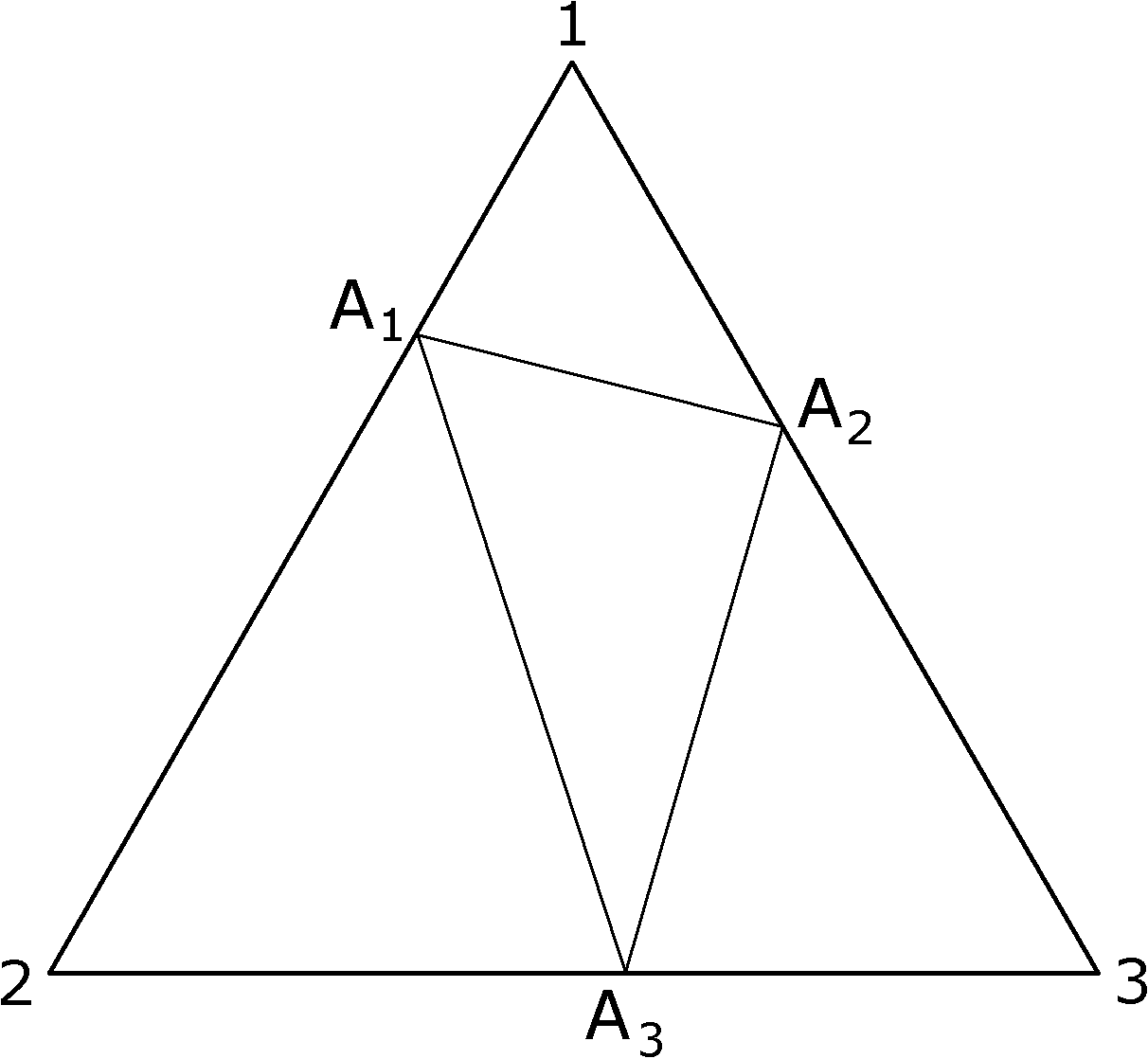
Figure 1: Triangle geometry of the qubit state.

and satisfy the inequality

$$a^{2}+b^{2}+c^{2}\leq 1.$$ (82)

The points with coordinates $a,b$, and $c$ are situated in the Bloch ball, and the points on the surface of Bloch sphere correspond to the pure states of qubits. One can illustrate the qubit states using triangle geometry and the triada of Malevich’s squares. The triangle $A_{1}A_{2}A_{3}$ inside the equilateral triangle with side equal to $\sqrt{2}$ is shown in Fig. 1.

The vertices of the triangle are determined by the probabilities $p_{1}$, $p_{2}$, and $p_{3}$ [49, 50]. The correspondence is related to the bijective map of the Bloch parameters and the probabilities (80). This map is illustrated by three squares (black, red, and white) shown in Fig. 2 and constructed using the sides of triangle $A_{1}A_{2}A_{3}$. The sum of the areas of the squares is expressed in terms of the probabilities

$$S=2[3(1-p_{1}-p_{2}-p_{3})+2p_{1}^{2}+2p_{2}^{2}+2p_{3}^{2}+p_{1}p_{2}+p_{2}p_{3}+p_{3}p_{1}].$$ (83)

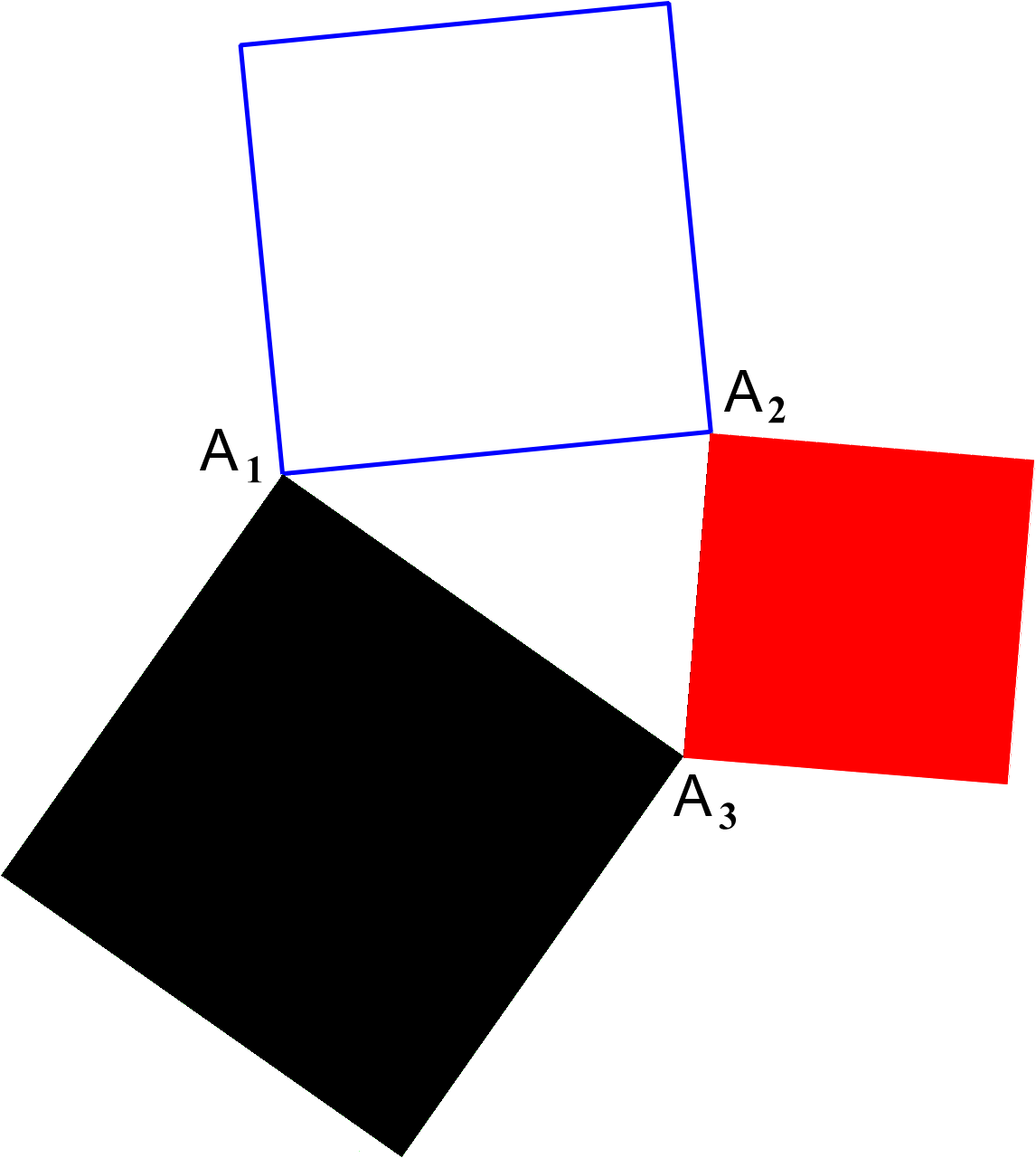
Figure 2: Triada of Malevich’s squares.

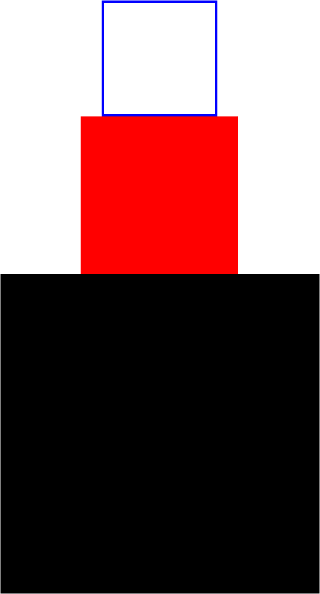
Figure 3: Three squares with different areas organized in the form of Malevich’s “tower” constructed of the three squares.

Thus, the point inside the Bloch ball is mapped onto the triada of squares called Malevich’s squares (see, Fig.2). The squares can be organized in the form of Malevich’s “tower” constructed of three squares; see Fig. 3. The maximum value of area $S$ for classical coin statistics is equal to $6$, which corresponds to the form of triangle $A_{1}A_{2}A_{3}$ coinciding with the equilateral triangle with the side $\sqrt{2}$. The quantization condition provides the maximum value of area $S=3$, which corresponds to the length of the side of the equilateral triangle $A_{1}A_{2}A_{3}$ equal to one. The approach to interpret the geometry of qubit states using the triangle and Malevich’s squares geometry was called the quantum suprematism picture of qubit states in [49, 50]. Thus, the quantization procedure suggested to connect classical coin statistics with quantum statistics of qubit states has a geometrical interpretation in terms of the triangle geometry and the geometry of the triada of Malevich’s squares. The quantization provides the prediction of quantum-to-classical ratio of areas $S_{\rm classical}/S_{\rm quantum}=6/3=2$. It can be checked experimentally measuring $p_{1}$, $p_{2}$, and $p_{3}$.

7 Conclusions

To conclude, we point out our main results.

We presented a review of a new approach to the formulation of quantum system states and observables, where the states are described by probabilities. We show that the qubit state can be given as a set of three probability distributions $(p_{1},1-p_{1})$, $(p_{2},1-p_{2})$, and $(p_{3},1-p_{3})$, describing three classical coins. We presented the superposition principle of the pure qubit states in the form of the addition rule of these probability distributions.

The quantization procedure of classical coin tossing game expressed as the condition for the coin probability distributions is suggested. The quantum observables (Hermitian matrices) are interpreted in terms of classical random variables. The addition rule for the probabilities can be illustrated as a rule of the combination of two triadas of Malevich’s squares. The extension of the obtained nonlinear addition rule for the probabilities determining the superpositions of arbitrary qudit states can be found.

One can illustrate the obtained bijective map of quantum states to the classical coin probabilities using the statement of Albert Einstein in the discussion with Niels Bohr on foundations of quantum mechanics “God does not play dice” and replacing it with the statement “God plays coins.”

References

- [1] L. D. Landau and E. M. Lifshitz, Mechanics. A Course of Theoretical Physics, Vol. 1, Pergamon Press (1969).
- [2] C. E. Shannon, Bell Syst. Tech. J., 27, 379 (1948).
- [3] A. S. Holevo, Statistical Structure of Quantum Theory, Lecture Notes in Physics, Springer, Berlin (2001).
- [4] A. S. Holevo, Probabilistic and Statistical Aspects of Quantum Theory, North Holland, Amsterdam (1982).
- [5] A. Khrennikov, Found. Phys., 35, 1655 (2005).
- [6] A. I. Khrennikov, Physica A, 393, 207 (2014).
- [7] A. Khrennikov and A. Alodjants, Entropy, 21, 157 (2019).
- [8] C. Tsallis, “Nonextensive statistical mechanics and themodynamics: Historical background and present status,” in: S. Abe and Y. Okamoto (Eds.), Nonextensive Statistical Mechanics and Its Applications, Lecture Notes in Physics, Springer, Berlin (2001), Vol. 560.
- [9] A. Rényi, Probability Theory, North-Holland, Amsterdam (1970).
- [10] E. Schrödinger, Ann. Phys. (Liepzig), 79, 489 (1926).
- [11] L. D. Landau, Z. Phys., 45, 430 (1927).
- [12] J. von Neuman, Nach. Ges. Wiss. Göttingen, 11, 245 (1927).
- [13] P. Dirac, The Principles of Quantum Mechanics, Oxford University Press (1930).
- [14] E. Wigner, Phys. Rev., 40, 749 (1932).
- [15] K. Husimi, Proc. Phys. Math. Soc. Jpn., 23, 264 (1940).
- [16] Y. Kano, J. Math. Phys., 6, 1913 (1986).
- [17] W. Heisenberg, Z. Phys., 43, 172 (1927).
- [18] E. Schrödinger, Ber. Kgl. Akad. Wiss., Berlin, 24, 296 (1930).
- [19] H. P. Robertson, Phys. Rev. A, 35, 667 (1930).
- [20] R. J. Glauber, Phys. Rev. Lett., 10, 84 (1963).
- [21] E. C. G. Sudarshan, Phys. Rev. Lett, 10, 84 (1963).
- [22] D. I. Blokhintsev, J. Phys. USSR, 2 (1), 71 (1940).
- [23] D. I. Blokhintsev, Sov. Phys. Uspekhi, 20 (8) 683(1977).
- [24] S. Mancini, V. I. Man’ko, and P. Tombesi, Phys. Lett. A, 213, 1 (1996).
- [25] J. Bertrand and P. Bertrand, Found. Phys., 17, 397 (1989).
- [26] K. Vogel and H. Risken, Phys. Rev. A, 40, 2847 (1989).
- [27] D. T. Smithey, M. Beck, M. G. Raymer, and A. Faridani, Phys. Rev. Lett., 70, 1244 (1993).
- [28] S. Mancini, V. I. Man’ko, and P. Tombesi, Found. Phys., 27, 801 (1997).
- [29] O. V. Man’ko and V. I. Man’ko, J. Russ. Laser Res., 18, 407 (1997).
- [30] J. Radon, Ber. Sächsische Akad. Wiss., 29, 262, Leipzig (1917).
- [31] O. V. Man’ko, V. I. Man’ko, and O. V. Pilyavets, J. Russ. Laser Res., 26, 429 (2005).
- [32] M. Asorey, A. Ibort, G. Marmo, and F. Ventriglia, Phys. Scr., 90, 074031 (2015).
- [33] G. G. Amosov, Ya. A. Korennoy, and V. I. Man’ko, Phys. Rev. A, 85, 052119 (2012).
- [34] Y. A. Korennoy and V. I. Man’ko, J. Russ. Laser Res., 32, 74 (2011).
- [35] O. V. Man’ko and V. N. Chernega, JETP Lett., 97, 557 (2013).
- [36] V. N. Chernega and O. V. Man’ko, J. Russ. Laser Res., 39, 411 (2918).
- [37] O. V. Man’ko and N. V. Tcherniega, J. Russ. Laser Res., 22, 201 (2001).
- [38] S. V. Kuznetsov, O. V. Man’ko, and N. V. Tcherniega, J. Opt. B: Quantum Semiclass. Opt., 5, 5503 (2003).
- [39] V. V. Dodonov and V. I. Man’ko, Phys. Lett. A, 239, 335 (1997).
- [40] V. I. Man’ko and O. V. Man’ko, J. Exp. Theor. Phys., 85, 430 (1997).
- [41] O. V. Man’ko, “Tomography of spin states and classical formulation of quantum mechanics,” in: B. Gruber and M. Ramek (Eds.), Proceedings of the International Conference “Symmetries in Science X” (Bregenz, Austria, 1997), Plenum Press, New York (1998), p. 207.
- [42] G. M. D’Ariano, L. Maccone, and M. Paini, J. Opt. B: Quantum Semiclass. Opt., 5, 77 (2003).
- [43] S. Weigert, Phys. Rev. Lett., 84, 802 (2000).
- [44] J.-P. Amiet and S. Weigert, J. Opt. B: Quantum Semiclass. Opt., 1, L5 (1999).
- [45] V. I. Man’ko, O. V. Man’ko, and S. S. Safonov, Theor. Math. Phys, 115, 520 (1998).
- [46] V. A. Andreev, O. V. Man’ko, V. I. Man’ko, and S. S. Safonov, J. Russ. Laser Res., 19, 340 (1998).
- [47] O. V. Man’ko, Acta Phys. Hung. A, 19, Nos. 3–4, 313 (2004).
- [48] S. N. Filippov and V. I. Man’ko, J. Russ. Laser Res., 34, 14 (2013).
- [49] V. N. Chernega, O. V. Man’ko, and V. I. Man’ko, J. Russ. Laser Res., 38, 416 (2017).
- [50] V. N. Chernega, O. V. Man’ko, and V. I. Man’ko, J. Phys. Conf. Ser., 1071, 012008 (2018).
- [51] V. N. Chernega, O. V. Man’ko, and V. I. Man’ko, J. Russ. Laser Res., 39, 128 (2018).
- [52] V. N. Chernega, O. V. Man’ko, and V. I. Man’ko, J. Russ. Laser Res., 38, 324 (2017).
- [53] V. N. Chernega, O. V. Man’ko, and V. I. Man’ko, J. Russ. Laser Res., 38, 141 (2017).
- [54] V. N. Chernega, O. V. Man’ko, and V. I. Man’ko, Eur. Phys. J. D, 73, 10 (2019).
- [55] M. A. Man’ko and V. I. Man’ko, Entropy, 17, 2876 (2015).
- [56] M. A. Man’ko and V. I. Man’ko, Entropy, 20, 692 (2018).
- [57] J. A. Lopez-Saldivar, O. Castaños, E. Nahmad-Achar, et al., Entropy, 20, 630 (2018).
- [58] V. I. Man’ko, G. Marmo, F. Ventriglia, and P. Vitale, J. Phys. A: Math. Theor., 50, 335302 (2017).
- [59] E. C. George Sudarshan, J. Russ. Laser Res., 24, 195 (2003).
- [60] B. O. Koopman Proc. Natl. Acad. Sci. USA, 17(5), 315(1931).
- [61] J. von Neuman, Ann. Math., 33, 587 (1932).
- [62] O. V. Man’ko and V. I. Man’ko, J. Russ. Laser Res., 22, 149(2001).
- [63] V. N. Chernega and V. I. Man’ko, J. Russ. Laser Res., 28,535(2007).
- [64] A. S. Avanesov and V. I. Man’ko, J. Russ. Laser Res., 34, 239(2013).
- [65] D. Chruściński, V. I. Man’ko, G. Marmo, and F. Ventriglia, Phys. Scr., 90, 115202 (2015).
- [66] M. A. Man’ko and V. I. Man’ko, J. Russ. Laser Res., 40, 6 (2019).