Spatial Point Pattern and Urban Morphology: Perspectives from Entropy, Complexity and Networks

Abstract

Spatial organisation of physical form of an urban system, or city, both manifests and influences the way its social form functions. Mathematical quantification of the spatial pattern of a city is, therefore, important for understanding various aspects of the system. In this work, a framework to characterise the spatial pattern of urban locations based on the idea of entropy maximisation is proposed. Three spatial length scales in the system with discerning interpretations in terms of the spatial arrangement of the locations are calculated. Using these length scales, two quantities are introduced to quantify the system’s spatial pattern, namely mass decoherence and space decoherence, whose combination enables the comparison of different cities in the world. The comparison reveals different types of urban morphology that could be attributed to the cities’ geographical background and development status.

I Introduction

Cities as complex systems Batty (2005, 2013); Bettencourt et al. (2007); Bettencourt and West (2010) have been a topic of research beyond the traditional discipline of urban studies. The idea of complexity in cities arises from the fact that they comprise many entities interacting with one another locally and generating global emergent patterns. Those interactions and the associated patterns have been shown to exhibit properties (e.g.  Bettencourt et al., 2007) similar to those observed in theoretical models developed in the fields of Statistical Physics or Mathematics. Quantitative tools from these fields, therefore, can be fruitfully applied toward constructing a framework for Science of cities.

Of the many aspects of studying cities, the spatial organisation of physical form, i.e. infrastructure elements, in a city provides a fundamental understanding of the city’s way of life. Various methods have been employed to tackle the problem of characterising spatial patterns of urban systems, including fractal dimension Batty and Longley (1994), land use patterns Decraene et al. (2013); Goh et al. (2016), street networks Barthélemy and Flammini (2008); Louf and Barthelemy (2014), or entropy of population density Volpati and Barthelemy (2018). Among them, percolation has proved to be a powerful and useful tool to study urban morphology Makse et al. (1998). In recent years, percolation method has becoming increasingly popular in analysing the spatial organisation of places in urban systems at various scales, from city Huynh et al. (2018); Huynh (2019), to nation Arcaute et al. (2016) and inter-country level Fluschnik et al. (2016). The application of percolation in such studies has so far been mainly concerned with studying the evolution of the giant cluster formed when the distance threshold $\rho$ for inter-point interaction changes. The growth of such cluster involves a transition from a segregate state where points are disconnected to an aggregate state in which a path exists between a pair of points located at opposite ends of the system. The identification of such transition regime is normally done via rate of growth of the giant cluster as the distance threshold increases. The profiles of such growth can be divided into $3$ parts, namely slow growth, rapid growth and stabilisation (Fig. 1). At small value of distance threshold, most clusters are localised due to limited connections with other nearby points. As $\rho$ increases, points can have access to farther neighbours, making small clusters merge to form larger ones. When $\rho$ is sufficiently large, a dominant cluster emerges and rapidly grows within a narrow range of $\rho$, known as transition regime Stauffer and Aharony (1994). After this regime, the dominant cluster, also called a giant cluster, starts to stabilise as it has already grasped most of the points and only grows slowly until no further expansion is possible, i.e. all points now belong to a single, unified cluster with a path existing between any pair of points in the set.

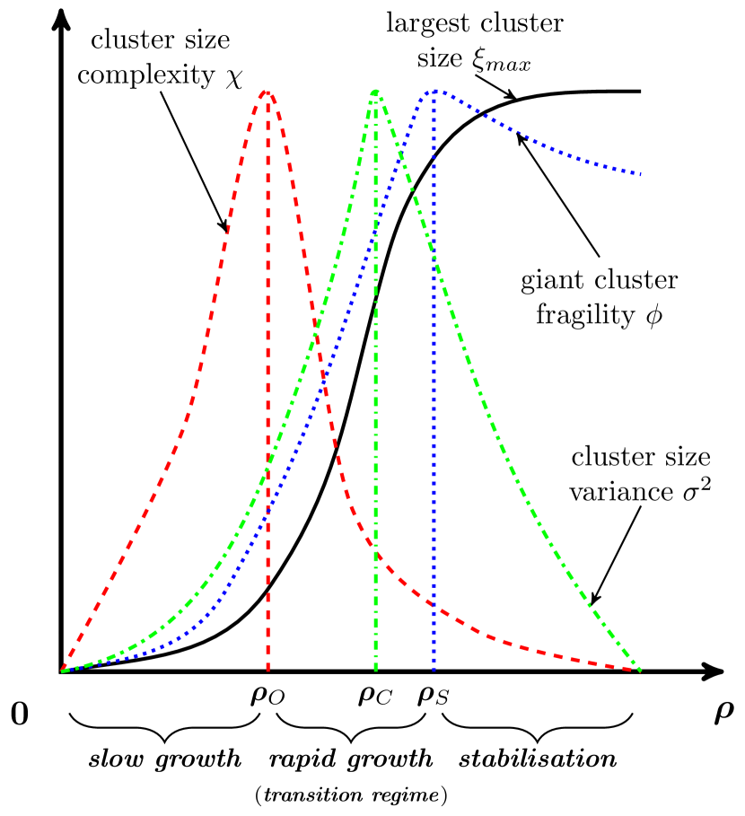
Figure 1: Growth of largest cluster in a set of points as the range of interaction among points increases. Three stages of growth could be observed, namely slow growth, rapid growth and stabilisation. As will be discussed in the text later, the window of rapid growth can be determined by two length scales that signify the maximisation of entropy measures of connected clusters ($\rho_{O}$ and red dashed curve) and robust components of the giant cluster ($\rho_{S}$ and blue dotted curve) as range of interaction $\rho$ changes. The rapid growth window also encompasses the transition of the system from segregate to aggregate state, represented by the percolation threshold $\rho_{C}$ at which the sizes of the clusters are most diverse (green dash-dot curve).

Traditionally, theoretical study of percolation on regularly spaced lattices provides procedures to quantify the transition regime and characterise it in the framework of universality classes Stauffer and Aharony (1994); Stanley (1999). Extending to continuous space, continuum percolation theory relaxes the position of points and studies their properties, including the conditions for existence of the giant cluster under different settings Gilbert (1961); Meester and Roy (1996). While a number of studies have been devoted to estimate the value of percolation threshold, especially in thermodynamic limit for theoretical systems (e.g.  Rintoul and Torquato, 1997; Mertens and Moore, 2012), much less focus has been put on determining the transition in a finite set of points, which could appear very fuzzy, especially in real data. In the context of urban studies, some measures have been applied to investigate the percolation transition in road networks Molinero et al. (2017), yet the transition regime in finite systems remains largely unexplored. Such result is particularly useful for practical applications like quantitative urban morphology, where data are always bounded.

This study, therefore, aims to present a framework to examine the transition in the context of continuum percolation of a finite set of points, by identifying different length scales associated with different states of the system as the distance threshold $\rho$ changes and combining them to quantify the transition. In the remaining of this paper, these length scales are calculated in Sec. II, which will be employed to characterise the transition growth of giant cluster via two measures of mass and space decoherence. The two measures will be used to assess different real urban systems in Sec. IV. Finally, discussions and summary are offered in Sec. V

II Length scales in continuum percolation process

II.1 Critical distance threshold

Drawing upon the an important property of percolation that physical quantities (e.g. correlation length) diverge, i.e. lack of characteristic size, at the critical point, it could be paralleled that the variance of cluster size (number of points in a cluster) maximises when the system experiences the most abrupt change in its state. In other words, the values of cluster size are most spread when the system transits across a “critical” point differentiating the aggregate and segregate state in the system Tsang and Tsang (1999); Tsang et al. (2000).

To make things concrete, let us consider a set of $N$ points in a two-dimensional domain $\mathbb{R}^{2}$. Given a distance threshold $\rho$, the set is divided into $n$ clusters of size $\xi_{i}$, which sum up to $N$, i.e.

$$\sum_{i=1}^{n}{\xi_{i}}=N\text{,}$$ (1)

and whose variance is given by $\sigma^{2}=\left\langle\xi^{2}\right\rangle-\left\langle\xi\right\rangle^{2}$. The value of distance threshold at which the variance $\sigma^{2}$ maximises is denoted $\rho_{C}$ to mark the critical point in the transition of the system (see green dash-dot curve in Fig. 1). This value is analogous with the percolation threshold in the classic percolation theory. As with percolation theory, the percolation threshold itself is not sufficient in characterising the phase transition in the system. Rather, the manner of transition is more important with many interesting properties. In what follows, it will be shown that the window of transition could be characterised by employing the measures of entropy. In particular, the measures of entropy can be used to quantify the pattern of clusters formed at every value of distance threshold and identify the length scales at which the entropy measures maximise. As will be argued later, these length scales correspond to the change of state of spatial agglomeration in the set of points.

II.2 Measures of fragmentation and complexity of clustering configuration

II.2.1 Measure of fragmentation

For the clusters in Eq. (1), the probability of choosing a random point $a$ that belongs to a cluster $C_{i}$ of size $\xi_{i}$, also the probability of picking the cluster $C_{i}$ itself, is simply given by the fraction of points in that cluster, $p_{i}=p(a\in C_{i})=\displaystyle\frac{\xi_{i}}{N}$. With this, we can easily calculate the Shannon entropy of the particular cluster division in Eq. (1)

$$S=-\sum_{i=1}^{n}{p_{i}\log{p_{i}}}=-\sum_{i=1}^{n}{\frac{\xi_{i}}{N}\log{\frac{\xi_{i}}{N}}}\text{.}$$ (2)

It could be seen from Eq. (2) that when there is a dominant cluster $C_{i^{\star}}$ of very large size alongside several tiny clusters of vanishingly small sizes (which are yet to be absorbed into the giant cluster), the entropy is close to $0$ since $\displaystyle\log{\frac{\xi_{i^{\star}}}{N}}\approx 0$ and $\displaystyle\frac{\xi_{i}}{N}\approx 0$, $\forall i\neq i^{\star}$. This reflects the state of division that the set of $N$ points is barely fragmented, where most of them belong to a single, unified cluster. On the other hand, it is a well-known fact for Shannon entropy formula that given $n$ events, the respective entropy is maximised when each of them takes place with equal probability $\displaystyle\frac{1}{n}$, which simply yields

$$\max{(S)}=-\sum_{i=1}^{n}{\frac{1}{n}\log{\frac{1}{n}}}=\log{n}\text{,}$$ (3)

i.e. the scenario of dividing the set of $N$ points into $n$ equal clusters. This is the state of maximal uncertainty since any of the clusters can be picked with equal probability. Equation (3) also indicates that the upper bound of entropy measure for $n$ events increases with the number of events. This points to the fact that maximal possible entropy in the system is $S_{max}=\log{N}$ when there are $N$ clusters, each of size $1$ and being picked with equal probability $\displaystyle\frac{1}{N}$. This corresponds to a state of being totally fragmented when each point forms its own cluster. In other words, the Shannon entropy in Eq. (2) can be interpreted as measure of fragmentation in the set of $N$ points. This is considered “first-order” measure in the sense that the formula operates directly on the size fraction of the individual clusters. In the following, we consider another measure that operates on the size distribution of the clusters.

II.2.2 Measure of complexity and onset of giant cluster formation

We again consider a set of $N$ points being divided into $n$ clusters of size $\xi_{i}$, which consist of points within distance $\rho$ of one another. Let’s denote $m(\xi)$ the number of clusters having size $\xi$ so that we have

$$\sum_{\xi=1}^{\xi_{max}}{m(\xi)\xi}=N\text{,}$$ (4)

in which $\xi_{max}$ is the size of the largest cluster. The probability of randomly choosing a point that belongs to a cluster of size $\xi$ is given by $\displaystyle P(\xi)=\frac{m(\xi)\xi}{N}$. With this, the entropy of cluster sizes could be calculated as

$$\chi=-\sum_{\xi=1}^{\xi_{max}}{P(\xi)\log{P(\xi)}}=-\sum_{\xi=1}^{\xi_{max}}{{\frac{m(\xi)\xi}{N}}{\log{\frac{m(\xi)\xi}{N}}}}\text{.}$$ (5)

When there are several tiny clusters of vanishingly small sizes alongside a dominant cluster $C_{i^{\star}}$ of very large size, i.e. very large $\rho$, the entropy $\chi$ is close to $0$ since $\displaystyle\log{\frac{m(\xi_{i^{\star}})\xi_{i^{\star}}}{N}}\approx 0$ (for $m(\xi_{i^{\star}})=1$ and $\xi_{i^{\star}}\approx N$) and $\displaystyle\frac{m(\xi)\xi}{N}\approx 0$, $\forall\xi\neq\xi_{i^{\star}}$. At the other extreme, when every point forms a cluster of its own, i.e. very small $\rho$, the probability of choosing a random point that belongs to a cluster of size $\xi$ is given by a Kronecker delta $P(\xi)=\delta_{1,\xi}$, for which the entropy $\chi$ is trivially $0$. This points to the fact that at either extreme of cluster formation, the set of points is divided into a trivial pattern when the size of a randomly picked cluster is not uncertain, yielding vanishing entropy measure, i.e.

$$\lim_{\rho\rightarrow 0}{\chi} =-P(m(\xi)=N,\xi=1)\log{P(m(\xi)=N,\xi=1)}$$ (6)

$$=0\text{,}$$

$$\lim_{\rho\rightarrow\infty}{\chi} =-P(m(\xi)=1,\xi=N)\log{P(m(\xi)=1,\xi=N)}$$

$$=0\text{.}$$

From this, it can be seen that the measure of entropy $\chi$ in Eq. (5) exhibits a maximum value at some finite value of $\rho$ when the clusters are formed with various sizes at which the proportion of points in different cluster sizes are most uniform. At this juncture, it could be pictured that each point in a cluster of size $\xi$ carries a label $\xi$ and the division of $N$ points into different label groups transits from trivial to non-trivial and back to trivial again, as $\rho$ changes.

While the entropy $S$ defined in Eq. (2) is interpreted as the measure of fragmentation of the clusters, the second entropy $\chi$ defined in Eq. (5) could be interpreted as the measure of complexity of the clusters’ pattern. The pattern is simple when most of the points carry the same label, i.e. indistinguishable, whereas a more complex pattern is produced when many labels are needed to describe the points. This complexity measure is useful because we can employ it to mark the onset of giant cluster formation as the value of $\rho$ changes. At small value of $\rho$, many small clusters exist but the number of labels is limited as the largest cluster size remains small (a fragmented pattern can be observed in top left panel of Fig. 2). When $\rho$ increases, the labels become more diverse when more cluster sizes come to existence with the lifting of the largest cluster size (a mixed pattern can be observed in middle left panel of Fig. 2). However, as $\rho$ progresses further, the largest cluster starts to grow by absorbing smaller ones, reducing the number of labels needed, and hence, decreasing the complexity $\chi$ of the clusters’ pattern (a simple pattern with a dominating cluster can be observed in bottom left panel of Fig. 2). Once the giant cluster has been formed, it continues to (slowly) absorb other smaller clusters, further reducing the number of labels and decreasing the complexity $\chi$, which eventually vanishes when only a single label is needed for all the points in a single cluster. The value of $\rho$ at which the complexity measure attains its maximum $\chi_{max}$ is denoted $\rho_{O}$ to mark the onset of giant cluster formation (see red dashed curve in Fig. 1), as reasoned above.

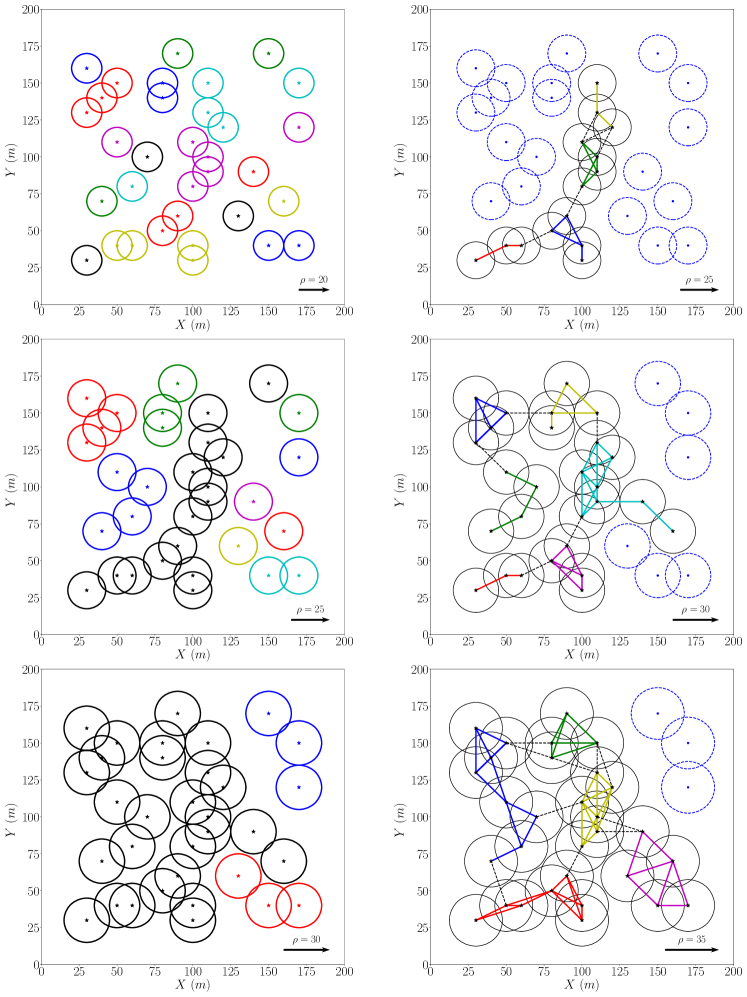
Figure 2: Illustration of complexity and fragility measures of the percolation clusters at different values of parameter distance (colours online). Left column: patterns of clusters to illustrate complexity measure. Right column: patterns of network formed by the giant cluster, whose communities are colour coded, to illustrate fragility measure. Top row: patterns slightly before the measures peak. Middle row: patterns when the measures peak. Bottom row: patterns slightly after the measures peak. For clear visuality, each points is surrounded by a circle of radius that is equal half the value of the distance parameter $\rho$. Any two overlapping (or touching) circles belong to the same cluster. These circles are not to be confused with the calculation of cluster area in Fig. 4.

II.3 Measure of fragility of giant cluster

The determination of clusters based on distance threshold indicates that there is a path between every pair of points of a cluster. It, however, does not tell how strongly connected the points are. In order to understand the internal structure of a cluster, pairwise connection between every pair of points in the cluster has to be taken into account.

To this end, a network of points’ connections within a cluster could be constructed (see right panels of Fig. 2), where a link between a pair of points, $a$ and $b$, exists if and only if their distance $d_{ab}$ is less than the threshold $\rho$. The strength $w_{ab}$ of connection between the pair is further taken into account in the form of the inverse of their distance, $w_{ab}\propto d_{ab}^{-1}$, i.e. a distant pair is less connected than a closer one. With this network, it could be examined which parts of the cluster are only weakly connected to the rest, using a community detection method Newman (2004), the Louvain method Blondel et al. (2008) in particular. Once the communities within a cluster have been identified, one can then apply the measure of fragmentation introduced in Eq. (2) to determine the fragility of a cluster. To do this, each of the identified communities is considered a sub-cluster within the larger cluster of interest (whose fragility is to be quantified), and the size of the sub-cluster enters Eq. (2) as $\xi_{i}$. If a cluster can be broken up into multiple tight-knit communities, it is said to be more fragile than a cluster that consists of only one or few closely connected communities.

Applying this to the giant cluster, it could be conceived that when the giant cluster grows, it initially only contains a few points that are closely connected to one another, yielding low fragility (only one or few tight-knit communities). When the giant cluster grows further, more points are added to the cluster, whose ties are not yet strengthened, producing multiple communities, and hence, high fragility. This trend continues into the transition regime, with increasing fragility. After the transition regime, most of the points are now part of the giant cluster, slowing down the cluster’s growth. At this point, with sufficiently large value of distance threshold $\rho$, points across different (distant) regions of the giant cluster can form links to strengthen the ties within the community they belong to, making the cluster more robust, or less fragile. The measure of fragmentation is useful in this case as the distance threshold $\rho$ at which the entropy $S$ peaks, denoted $\rho_{S}$, is a good indicator of the onset of stabilisation of the giant cluster (see blue dotted curve in Fig. 1). This is where the giant cluster is most fragile to be broken into components.

It should be remarked that the size of giant cluster changes with the distance parameter. In practice, to make its fragility measure comparable across different values of $\rho$, the sum of all the sub-clusters in Eq. (2) is kept constant by lumping the remaining points (outside the giant cluster) as a single cluster whose size also contributes an extra term in Eq. (2). This treatment also helps to take care of the scenario where multiple robust clusters (almost fully connected, and of similar sizes) have been established but are not yet connected to form a giant cluster. As $\rho$ increases, the overall fragility should increase and peaks when these clusters merge, where the newly formed giant cluster only has loosely connected components. In most other cases, this has mild effect after the giant cluster has been formed as the number of non-giant-cluster points is much smaller than the size of the giant cluster itself.

As an example for illustration, right panels of Fig. 2 show the networks formed by points in the giant cluster at different values of the distance parameter $\rho$, right before, at, and after the peak value for the fragility measure. The points in the giant cluster are surrounded with black solid circles, whereas the others are marked with blue dashed circles. Within the giant cluster, any pair of points whose distance is less than or equal to distance threshold is linked by a line, which makes an edge of the corresponding network. The communities in this network, identified using Louvain method, are colour-coded in the plots for clarity, with intracommunity links represented as coloured solid lines and intercommunity ones as black dashed lines. There are in total $N=33$ points in the entire set. At $\rho=25m$, the giant cluster contains $14$ points divided into 4 sub-clusters of size $(4,4,3,3)$, leaving $19$ points outside. Hence, the corresponding fragility measure is $\phi_{\xi}=1.265$. Similarly, at $\rho=30m$, the sub-cluster sizes are $(8,4,4,4,4,3)$, yielding $\phi_{\xi}=1.895$. Finally, at $\rho=35m$, the sub-cluster sizes are $(8,7,6,5,4)$, yielding $\phi_{\xi}=1.742$.

II.4 Effective width of transition window

The two distance scales $\rho_{O}$ and $\rho_{S}$ discussed above can be used to determined the window of rapid growth of the giant cluster across the transition of the system from segregate to aggregate state. Further combination with the critical percolation distance $\rho_{C}$ would enable calculation of the effective width of transition window, which characterises how the system transits from segregate to aggregate state. To do this, it is noted that a linear growth of the giant cluster between $\rho_{O}$ and $\rho_{C}$ should indicate a longer effective width than that of an exponential-like growth. For this, it is useful to use the ratio between the area $\mathcal{F}_{1}$ under the growth curve of giant cluster and the change in cluster size $\xi_{C}-\xi_{O}$ as the effective width (see Fig. 3). Similarly, the effective width after the critical distance, between $\rho_{C}$ and $\rho_{S}$ could be calculated in the same manner. Subsequently, the effective width $\omega$ of the transition window $\omega$ is simply the sum of widths both before and after the critical percolation threshold

$$\omega=\delta(\rho_{O},\rho_{C})+\delta(\rho_{C},\rho_{S})=\frac{\mathcal{F}_{1}}{\xi_{C}-\xi_{O}}+\frac{\mathcal{F}_{2}}{\xi_{S}-\xi_{C}}\text{.}$$ (7)

This effective width is useful for it characterises the sharpness of transition or the growth of the largest cluster, similar to the critical exponents that characterise the divergence of a system’s physical quantities (e.g. correlation length, average cluster size, etc…) in standard percolation theory. For the purpose of comparing different systems, a dimensionless width rescaled by the critical percolation threshold is used

$$\epsilon=\frac{\omega}{\rho_{C}}\text{.}$$ (8)

It could be seen that this quantity indeed provides a measure of “decoherence” of relative distance among points in a set. In other words, if the points are regularly spaced, their relative distances are mostly uniform, i.e. more coherent, yielding a small value of $\epsilon$. However, if the points are scattered with inter-point distances ranging a wide spectrum, i.e. less coherent, the value of $\epsilon$ would surge.

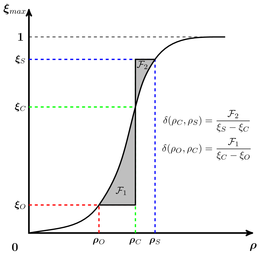
Figure 3: Calculation of effective width of transition window before (marked by $\rho_{O}$) and after (marked by $\rho_{S}$) the critical value $\rho_{C}$ of percolation threshold.

II.5 Mass decoherence vs. space decoherence

It should be noted that the discussion so far has been concerned with the measure of size (or mass) of the clusters formed in the continuum percolation process. As have been previously shown Huynh et al. (2018); Huynh (2019), the area of clusters, i.e. their spatial extent, provides a different perspective to understand the (relative) spatial arrangement of points in a domain.

The area measure $A$ of a cluster of points, formed via percolation at distance parameter $\rho$, is defined as the union area of all the circles of radius $\rho$ centred at those points, normalised by the area of a single such circle (see Fig. 4). The normalisation is needed to emphasise the fact that the cluster area measures the compactness of the set of points, that as the larger $\rho$ gets, the cluster area does not necessarily expand unless new points are grasped by the cluster. This definition of cluster area is also dimensionless and directly comparable with the size of the cluster, i.e. number of points in the cluster, which makes all the measures discussed above conveniently extended to cluster area. It could be easily proven that the area $A$ of a cluster (in this definition) is always smaller than its size $\xi$ due to the non-tiling nature of circles when packed to fill space. As illustrated in Fig. 4, a cluster of a fixed size $\xi$ takes different values for its area $A$ for different arrangements, with the more compact one (smaller average nearest-neighbour distance, see lower panel of Fig. 4) possessing smaller area.

Figure 4: Calculation of area measure of a cluster of points. In the upper panel, $6$ points ($\xi=6$) are arranged in a $2\times 3$ lattice of spacing $d=1$, i.e. the nearest-neighbour distance of every point is $1$. In the lower one, the points’ nearest-neighbour distance is either $1$ or $\displaystyle\frac{1}{\sqrt{2}}$, in the form of an isosceles right triangle. In both cases, the parameter distance is set at $\rho=1.1$, sufficient to have all the points belong to a single cluster. The area measure $A$ is the union area (dotted) of all the circles of radius $\rho$, normalised by the area of a single circle. Simple calculations yield the values $\displaystyle A=4+\frac{8r^{2}}{\pi}+\frac{6r}{\pi}\sqrt{1-r^{2}}-\frac{6}{\pi}\cos^{-1}{r}\approx 3.201$ and $\displaystyle A=4+\frac{4r^{2}}{\pi}+\frac{2r}{\pi}\sqrt{1-r^{2}}+\frac{2r}{\pi}\sqrt{2-r^{2}}-2\cos^{-1}{r}-4\cos^{-1}{\frac{r}{\sqrt{2}}}\approx 2.625$, respectively with $\displaystyle r=\frac{d}{2\rho}=\frac{1}{2.2}$.

The measures of size and area complement one another and their combination can be employed to distinguish different types of spatial point distribution. In the following discussion, $\epsilon_{A}$ and $\epsilon_{\xi}$ are used to denote the normalised spread in Eq. (8) calculated for cluster area and cluster size, respectively. Hereafter, the subscripts $A$ and $\xi$ also correspondingly denote other quantities with respect to cluster area and cluster size. On the one hand cluster size measures the amount of points contained in the cluster and can be interpreted as mass, on the other hand cluster area measures the (two-dimensional) space (continuously) occupied by the points of the cluster and can be interpreted as spatial extent. For that, we shall term $\epsilon_{A}$ space decoherence and $\epsilon_{\xi}$ mass decoherence.

III Transition window of different types of point pattern

To illustrate the framework developed in Sec. II, two artificial point patterns are analysed in details, showing the growth profiles of the largest cluster in terms of both the cluster area and size. The effective width of transition window is also calculated for each of the simulated point patterns, which will then be used to calculate the decoherence measures. The two point patterns are examples of homogenous pattern with approximately equal nearest-neighbour distance and inhomogeneous pattern whose density of points varies.

III.1 Homogeneous point pattern

As an example of homogeneous point pattern, the points are generated by randomly displacing the sites of a regular square lattice (see top left panel of Fig. 5). The amplitude of displacement applied is sufficient but not more than the lattice spacing. The growth of both the largest cluster area and size (middle and bottom left panels of Fig. 5, respectively) is probed by gradually increasing the distance parameter $\rho$. It could be observed that there is an abrupt increase in both the largest cluster size and area around $\rho_{C}=125m$, which is the inverse of the linear density of the point pattern, i.e. square root of the number of points per unit area ($1,024$ over $4,000m\times 4,000m$). The complexity measures peak rapidly when $\rho$ approaches (just before) the critical distance threshold, and drop sharply as $\rho$ increases beyond $\rho_{C}$. The fragility measures of the giant cluster, on the other hand, also peak rapidly right after $\rho_{C}$ but gradually decrease further after that. If one reverses the process, tracing the fragility measures as $\rho$ decreases, it could be seen that more (long-range) links are removed from the network formed by the giant cluster, making it more fragile. Slightly above the critical distance $\rho_{C}$, the giant cluster quickly becomes disintegrated, broken up into smaller clusters, of which the largest cluster is now much smaller but more robust. The window of transition for the point pattern, marked by the peaks of complexity and fragility measures, is narrow for both cluster size and area. The decoherence measures as defined in Eq. (8) are both very small with space decoherence $\epsilon_{A}=0.037$ and mass decoherence $\epsilon_{\xi}=0.034$.

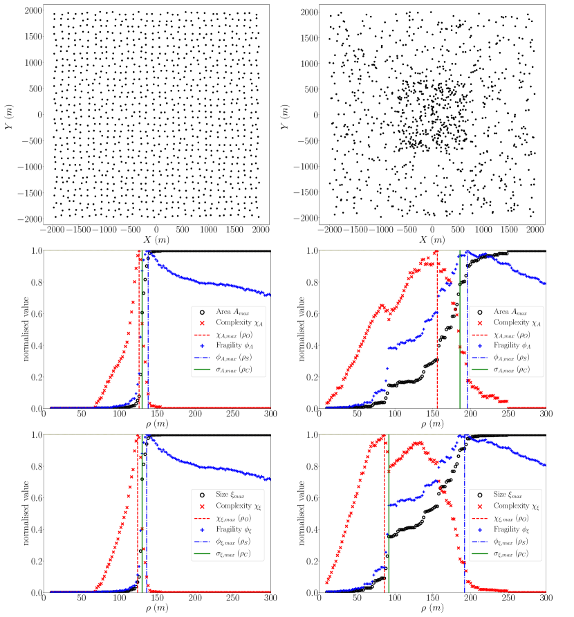
Figure 5: Application of the measures in Sec. II to simulated point patterns (colours online). Left column: results for a homogeneous point pattern, which is obtained by adding noise to a regular square lattice pattern. Right column: results for an inhomogeneous point pattern, whose density varies with more points concentrating near the centre. Top row: distribution of points in a domain of size $4,000m\times 4,000m$, with $1,024$ ($32\times 32$) points on the left and $1,000$ points on the right. Middle row: growth profile of the largest cluster area, with vertical lines marking the length scales described in Sec. II. Bottom row: growth profile of the largest cluster size, with vertical lines marking the corresponding length scales, namely maximum complexity (onset of giant cluster, $\rho_{O}$), maximum diversity (critical distance, $\rho_{C}$) and maximum fragility (stabilisation of giant cluster, $\rho_{S}$). The homogeneous pattern exhibits a sharp growth of both largest cluster area and size and consequently a narrow window of transition, whereas the inhomogeneous pattern produces a gradual growth of both largest cluster area and size resulting in a wide window of transition.

III.2 Inhomogeneous point pattern

For inhomogeneous point pattern, a simple example is obtained by having more points concentrated in the centre region, whose density is about $4$ times more than the rest. As the distance parameter $\rho$ increases, the growth of both largest cluster cluster size and area shows gradual increase pattern. Since the points tend to be clustered in the centre region (higher density, shorter nearest-neighbour distance), the largest cluster size grows faster than the area counterpart (see bottom and middle right panels of Fig. 5, respectively) as more points covering the same area compared to a lower-density pattern. Due to the faster growth pattern, the complexity measure for cluster size peaks earlier than that for cluster area. On the other hand, the fragility measure of the giant cluster only peaks once many points have been (loosely) encompassed by the cluster when $\rho$ reaches a sufficiently large value, before declining when the giant cluster becomes more robust with more long-range links allowed to establish at large values of $\rho$. As a result, the transition window for the point pattern is wide for both cluster size and area, with the latter being narrower due to the initial slower growth. The corresponding decoherence measures are $\epsilon_{A}=0.114$ and $\epsilon_{\xi}=0.731$, for space and mass, respectively.

IV Application to real urban locations data

In what follows, the two measures of space and mass decoherence are applied to a set of $39$ cities in the world to compare the spatial patterns of their urban morphology. The set of $39$ cities is drawn from the list of top $44$ cities ranked by the Global Power City Index (GPCI) 201 (2018). The data on spatial locations of the cities’ public transport nodes were either obtained from Open Street Map via Nextzen project Nex or from General Transit Feed Specification sources Tra . A small number ($5$) of cities were excluded since reliable data could not be obtained. Due to geographical features, some cities are divided into multiple parts by large water bodies (wide rivers or large bays or even open sea). As a result, the quantification of spatial pattern is reported for a total of $49$ sets of points (see Fig. 6).

Figure 6: Measures of mass and space decoherence of $49$ sets of public transport nodes from $39$ global cities 201 (2018). Some cities are split into multiple parts due to geography. General patterns could be observed where American and European cities flock in the lower left corner of the plot together with highly developed Asian cities from Japan, South Korea and Singapore, while other cities are found scattered.

Using the measures of mass and space decoherence to quantify spatial patterns of points, $3$ regions could be highlighted, namely highly coherent ($\epsilon_{A},\epsilon_{\xi}\lesssim 0.15$), coherent ($0.15\lesssim\epsilon_{A},\epsilon_{\xi}\lesssim 0.5$) and decoherent ($\epsilon_{A}\gtrsim 0.5$ or $\epsilon_{\xi}\gtrsim 0.5$). When the points are decoherent, their pattern can further classified as clustered or dispersed if one of the two measures is significantly smaller than the other (same reasoning for $\sigma_{A}$ and $\sigma_{\xi}$ in Huynh et al. (2018)).

From the spatial pattern of $49$ sets, it could be observed that most of American and European cities possess coherent spatial patterns with values of $\epsilon_{A}$ and $\epsilon_{\xi}$ not exceeding $0.5$. The borderline case of Los Angeles ($\epsilon_{\xi}\approx 0.5$) appears to support the perception that it is one of the most sprawling cities in the U.S. Bruegmann (2006). Quite a number of Asian cities also belong to this group of coherent spatial patterns, all of which are from developed countries and ranked very high by GPCI, like Tokyo (3), Singapore (5) or Seoul (7). The decoherent group with either $\epsilon_{A}>0.5$ or $\epsilon_{\xi}>0.5$ contains cities mostly from developing countries like Egypt, India or those in Southeast Asia. It is worth mentioning that different parts of the same city divided by geography like water bodies can possess very different morphologies. For example, the different boroughs in New York city possess patterns ranging from high coherence of grid-like street pattern (Manhattan) to decoherence of unplanned Staten Island. Another interesting example is Istanbul where the Asian part east of the Bosporus strait appears more coherent than its European portion in the west, which has been noted in literature and could be explained by the major urban growth in Anatolian Istanbul in the later half of last century Miyamoto et al. (2004). Further observations also suggest that cities known to be well-planned (and generally ranked high by GPCI) appear to possess small decoherence values, while the ones known for being sprawling (with tendency of lower GPCI rank) exhibit large space and/or mass decoherence, which could either have clustered ($\epsilon_{\xi}\gg\epsilon_{A}$) or dispersed ($\epsilon_{\xi}\ll\epsilon_{A}$) patterns.

V Conclusions

In summary, this work illustrates that patterns of points embedded in two-dimensional space can be quantified using measures of complexity of the set of points and fragility of the giant cluster in the set, formed via a continuum percolation process. Although many sophisticated techniques have been developed for understanding different types of spatial data Cressie and Wikle (2011), the general framework of percolation proves to provide a powerful toolbox to study spatial organisation of point pattern, providing a different perspective from that of common techniques of point pattern analysis. While point pattern analysis mostly deals with whether a collection of points exhibit complete spatial randomness (CSR), uniform or clustered patterns, continuum percolation on the other hand, explores the structure of points’ locations based on global distribution, via the growth of the largest, dominating cluster in the system. This growth is typically characterised by three stages of initial and final slow expansion, sandwiching a rapid development region that embraces all the interesting properties of a phase transition. Here, it is shown that window of the transition could be determined by two length scales concerning the complexity measure of the entire system, which marks the onset of the existence of dominant cluster, and the component entropy of the giant cluster, which measures its fragmentation or fragility. The former is the point at which the complexity measure of connected clusters is maximum, while the latter is where the giant cluster is most fragile to be broken into components, from a perspective of network presentation of clusters. The two length scales together with a third length scale, at which clusters are most diverse in the spirit of critical phase transition, allow the characterisation of transition of the system across the critical regime, in the form of decoherence measure. The combination of mass decoherence (for amount of points accumulated) and space decoherence (for spatial extent of points accumulated) can be employed to quantify the pattern of a set of spatial locations, enabling comparison among different sets. Applying this framework to the set of public transport nodes in cities in the world from both developed and developing countries, different types of spatial pattern can be discerned and attributed to the cities’ economical and geographical backgrounds. It is also worth mentioning that the framework could be applied to any point data sets in urban context, e.g. building locations, road junctions etc…, not necessarily restricted to public transport nodes.

As a final note, the term “complexity” in this work is inspired by a previous study of statistical complexity measure Crutchfield and Young (1989), in which two measures of metric entropy $h$ and statistical complexity $C_{S}$ were calculated for non-linear dynamical systems. The measure of fragmentation $S$ in Eq. (2) is similar to $h$, measure of randomness, which maximises at one extreme of the system parameter and vanishes at the other; whereas the measure of cluster size entropy $\chi$ in Eq. (5) is similar to $C_{S}$, measure of complexity, which peaks at some intermediate value of the system parameter, suggesting the idea that a system is most complex at the interface of different states.

References

- Batty (2005) M. Batty, Cities and Complexity (The MIT Press, Cambridge, 2005).
- Batty (2013) M. Batty, The New Science of Cities (The MIT Press, Cambridge, 2013).
- Bettencourt et al. (2007) L. M. A. Bettencourt, J. Lobo, D. Helbing, C. Kühnert, and G. B. West, P. Natl. Acad. Sci. 104, 7301 (2007).
- Bettencourt and West (2010) L. M. A. Bettencourt and G. B. West, Nature 467, 912– (2010).
- Batty and Longley (1994) M. Batty and P. Longley, Fractal Cities: A Geometry of Form and Function (Academic Press, London, 1994).
- Decraene et al. (2013) J. Decraene, C. Monterola, G. K. K. Lee, T. G. G. Hung, and M. Batty, PLoS ONE 8, 1 (2013).
- Goh et al. (2016) S. Goh, M. Y. Choi, K. Lee, and K.-M. Kim, Phys. Rev. E 93, 052309 (2016).
- Barthélemy and Flammini (2008) M. Barthélemy and A. Flammini, Phys. Rev. Lett. 100, 138702 (2008).
- Louf and Barthelemy (2014) R. Louf and M. Barthelemy, J. Roy. Soc. Interface 11 (2014).
- Volpati and Barthelemy (2018) V. Volpati and M. Barthelemy, arXiv e-prints 1804, arXiv:1804.00855 (2018).
- Makse et al. (1998) H. A. Makse, J. S. Andrade, M. Batty, S. Havlin, and H. E. Stanley, Phys. Rev. E 58, 7054 (1998).
- Huynh et al. (2018) H. N. Huynh, E. Makarov, E. F. Legara, C. Monterola, and L. Y. Chew, J. Comput. Sci. 24, 34 (2018).
- Huynh (2019) H. N. Huynh, “Continuum percolation and spatial point pattern in application to urban morphology,” in The Mathematics of Urban Morphology, edited by L. D’Acci (Springer International Publishing, Cham, 2019) pp. 411–429.
- Arcaute et al. (2016) E. Arcaute, C. Molinero, E. Hatna, R. Murcio, C. Vargas-Ruiz, A. P. Masucci, and M. Batty, Roy. Soc. Open Sci. 3, 150691 (2016).
- Fluschnik et al. (2016) T. Fluschnik, S. Kriewald, A. García Cantú Ros, B. Zhou, D. E. Reusser, J. P. Kropp, and D. Rybski, ISPRS International Journal of Geo-Information 5, 110 (2016).
- Note (1) A pair of points belong to the same cluster if and only if the distance between them is not more than the threshold , i.e. one can hop from one point in the cluster to any other points in the same cluster after jumping a finite number of times, each time a distance no more than .
- Stauffer and Aharony (1994) D. Stauffer and A. Aharony, Introduction to percolation theory (Taylor & Francis, London, 1994).
- Stanley (1999) H. E. Stanley, Rev. Mod. Phys. 71, S358 (1999).
- Gilbert (1961) E. Gilbert, J. Soc. Ind. Appl. Math. 9, 533 (1961).
- Meester and Roy (1996) R. Meester and R. Roy, Continuum Percolation, Cambridge Tracts in Mathematics (Cambridge University Press, 1996).
- Rintoul and Torquato (1997) M. D. Rintoul and S. Torquato, J. Phys. A Math. Gen. 30, L585 (1997).
- Mertens and Moore (2012) S. Mertens and C. Moore, Phys. Rev. E 86, 061109 (2012).
- Molinero et al. (2017) C. Molinero, R. Murcio, and E. Arcaute, Sci. Rep. 7, 4312 (2017).
- Tsang and Tsang (1999) I. R. Tsang and I. J. Tsang, Phys. Rev. E 60, 2684 (1999).
- Tsang et al. (2000) I. J. Tsang, I. R. Tsang, and D. V. Dyck, Phys. Rev. E 62, 6004 (2000).
- Newman (2004) M. E. J. Newman, Phys. Rev. E. 69, 066133 (2004).
- Blondel et al. (2008) V. D. Blondel, J.-L. Guillaume, R. Lambiotte, and E. Lefebvre, J. Stat. Mech. 2008, P10008 (2008).
- 201 (2018) “Global Power City Index 2018 by Institute for Urban Strategies, The Mori Memorial Foundation,” (2018).
- (29) “Nextzen metro extracts,” https://www.nextzen.org.
- (30) “Open mobility data,” https://transitfeeds.com.
- Bruegmann (2006) R. Bruegmann, Sprawl: A Compact History (University of Chicago Press, 2006) p. 133.
- Miyamoto et al. (2004) K. Miyamoto, S. R. Acharya, M. A. Aziz, J.-M. Cusset, T. F. Fwa, H. Gerçek, A. S. Huzayyin, B. James, H. Kato, H. D. Le, S. Lee, F. J. Martinez, D. Mignot, K. Miyamoto, J. Monigl, A. N. Musso, F. Nakamura, J.-P. Nicolas, O. Osman, A. Páez, R. Quijada, W. Schade, Y. Tanaboriboon, M. A. P. Taylor, K. N. Vergel, Z. Yang, and R. Zito, “Transport-environment issues and countermeasures in various metropolises,” in Urban Transport and the Environment: An International Perspective, edited by World Conference On Transport Research Society (Emerald Group Publishing Limited, 2004) Chap. 5, pp. 253–402.
- Cressie and Wikle (2011) N. A. C. Cressie and C. K. Wikle, Statistics for spatio-temporal data (Wiley, 2011).
- Crutchfield and Young (1989) J. P. Crutchfield and K. Young, Phys. Rev. Lett. 63, 105 (1989).