Coherence quantifiers from the viewpoint of their decreases in the measurement process

Abstract

Measurements can be considered as a genuine example of processes that crush quantum coherence. In the case of an observable with degeneracy, the formulations of Lüders and von Neumann are known. These pictures postulate the two different states of a system immediately following the act of measurement. Hence, they are associated with divers variants of coherence losses during the measurement. Recent studies have focused on several ways to characterize quantum coherence appropriately. One of the existing types of quantifier is based on quantum $\alpha$-divergences of the Tsallis type. In this paper, we introduce coherence quantifiers associated with the Lüders picture of quantum measurements. The are shown to satisfy the same properties as coherence $\alpha$-quantifiers related to some orthonormal basis. Further, we consider losses of quantum coherence during a generalized measurement. The proposed approach is exemplified with unambiguous state discrimination; extreme properties of the states to be discriminated are clearly shown.

I Introduction

Theoretical and experimental studies of coherence has a long history in physics. Complete understanding of this concept could be reached only within a purely quantum approach. In effect, recent investigations of coherence are connected with modern prospective technologies including quantum computations and quantum cryptography. One of genuine features of coherence-like quantities is that they are basis dependent. In many physical cases of interest, only a limited number of bases actually have a priority. This claim is quite obvious in application to quantum systems of information processing. The quantum parallelism of Deutsch deutsch is realized through quantum superpositions written in the prescribed basis. The concept of the pointer basis plays an important role in our treatment of measurement process zurek81 . Thermodynamic properties of nano-systems at low temperatures are commonly considered with the use of concrete representation for statistical mixtures horodecki15 ; ngour15 . Contemporary advances in theoretical studies of quantum correlations are reviewed in adesso16jpa ; fan2017 .

The characteristics of coherence and decoherence seem to be opposite to each other. Hence, various coherence quantifiers could be examined from the viewpoint of their decrease during processes with deep decoherence. The authors of yao17 have noted that quantum measurements are a quite typical example of such processes. If we adopt, here, the projection postulate, then this consideration leads us to one of the very core questions of quantum mechanics. The actual state right after measuring a degenerate observable can be given in two different forms, due to von Neumann and Lüders, respectively. The reduction rule of von Neumann appeals to the fact that each measurement uses a particular apparatus. Instead of the degenerate observable per se, we actually deal with its refinement (see section V.1 in neumann32 ). The latter commutes with the former, but has only non-degenerate eigenvalues. There is an obvious freedom in the choice of such refinements. Lüders luders51 has criticized von Neumann’s anzatz and replaced it with another one. Nowadays, the Lüders formulation of the projection postulate is most commonly used.

The relative entropy of coherence and the $\ell_{1}$-norm of coherence are widely applied due to their useful properties bcp14 . The authors of yao17 extended these quantities to measurements of the Lüders type, and mentioned the hierarchy relations showing a residual coherence. One family of coherence quantifiers is based on quantum $\alpha$-divergences of the Tsallis type. In this work, we aim to extend this concept to the case of Lüders-type measurements. Together with distance-based quantifiers of coherence, other quantities deserve to be considered. In particular, the robustness of coherence robcoh16 and the coherence weight anand17 have recently been proposed. The problem of maximizing coherence with respect to the reference bases was addressed in yao16 ; hsfan17 . It turned out that bases mutually unbiased with the state eigenbasis are optimal for the robustness of coherence and the coherence weight. Generalized quantum measurements are indispensable in quantum information processing. Basic ways of quantifying coherence can be extended to measurements described by positive operator-valued measures (POVMs). We will illustrate these proposals with unambiguous state discrimination, which is a very important and intuitively understandable example of a rank-one POVM.

The paper is organized as follows. In section II, we review the required material and fix the notation. Some standard results about quantum operations and measurements will be used throughout the paper. In particular, we recall both the von Neumann and Lüders approaches to measure an observable with degenerate eigenvalues. Section III is devoted to coherence quantifiers on the base of quantum Tsallis $\alpha$-divergences as applicatied to the Lüders picture. Basic properties of such quantifiers are discussed. The so-called residual coherence can be characterized by means of various coherence measures. Using the example of a concrete spin observable with a degenerate eigenvalue, we compare the level of residual coherence predicted by several quantifiers. In section IV, we address the question how to characterize losses of quantum coherence during a generalized quantum measurement. In the case of rank-one POVMs, we propose a natural approach realized through orthonormal bases in a suitably extended space. This approach is exemplified with the measurement designed for unambiguous state discrimination. In section V, we conclude the paper.

II Preliminaries

In this section, we begin by recalling the required formal definitions. Let $\mathcal{L}(\mathcal{H})$ be the space of linear operators on finite-dimensional Hilbert space $\mathcal{H}$. By ${\mathcal{L}}_{+}(\mathcal{H})$ and ${\mathcal{L}}_{s.a.}(\mathcal{H})$, we denote respectively the set of positive semidefinite operators and the real space of Hermitian ones. A state of the quantum system of interest is represented by the density matrix $\boldsymbol{\rho}\in{\mathcal{L}}_{+}(\mathcal{H})$ normalized as ${\mathrm{tr}}(\boldsymbol{\rho})=1$. Such matrices form the convex set ${\mathcal{D}}(\mathcal{H})$ of density operators acting on $\mathcal{H}$. The range of ${\mathsf{A}}\in\mathcal{L}(\mathcal{H})$ will be denoted as ${\mathrm{ran}}({\mathsf{A}})$. For ${\mathsf{A}}\in{\mathcal{L}}_{+}(\mathcal{H})$, we define ${\mathsf{A}}^{0}$ as the orthogonal projector onto ${\mathrm{ran}}({\mathsf{A}})$. In finite dimensions, we treat ${\mathsf{A}}^{0}\vee{\mathsf{B}}^{0}$ as the projector onto the sum of subspaces ${\mathrm{ran}}({\mathsf{A}})+{\mathrm{ran}}({\mathsf{B}})$. In the infinite-dimensional case, this definition should be modified. In the following, we will deal with the finite-dimensional case only. A distance between operators can be characterized by appropriately chosen norms. With respect to the given orthonormal basis, each operator ${\mathsf{A}}\in\mathcal{L}(\mathcal{H})$ is represented by the square matrix with elements $a_{ij}$. The $\ell_{1}$-norm is then defined as hornJ

$$\|{\mathsf{A}}\|_{\ell_{1}}:=\sum\nolimits_{ij}|a_{ij}|\,.$$ (1)

There are many norms that can be used to define measures of distinguishability of quantum states watrous1 . The well-known norm (1) gives the so-called $\ell_{1}$-norm of coherence bcp14 .

Another approach to compare quantum states is based on the notion of quantum relative entropy, or divergence. This concept is fundamental in quantum information theory nielsen ; vedral02 . For $\boldsymbol{\rho},\boldsymbol{\varrho}\in{\mathcal{D}}(\mathcal{H})$, the relative entropy of $\boldsymbol{\rho}$ with respect to $\boldsymbol{\varrho}$ is written as hmpb11

$${\mathrm{D}}_{1}(\boldsymbol{\rho}||\boldsymbol{\varrho}):=\begin{cases}{\mathrm{tr}}(\boldsymbol{\rho}\ln\boldsymbol{\rho}-\boldsymbol{\rho}\ln\boldsymbol{\varrho})\,,&\text{if ${\mathrm{ran}}(\boldsymbol{\rho})\subseteq{\mathrm{ran}}(\boldsymbol{\varrho})$}\,,\\ +\infty\,,&\text{otherwise}\,.\end{cases}$$ (2)

It is a quantum counterpart of the standard relative entropy of probability distributions. For the given probability distributions $\{p_{j}\}$ and $\{q_{j}\}$, it is defined by nielsen

$$D_{1}(p_{j}||q_{j}):=\sum\nolimits_{j}p_{j}\,\ln\frac{p_{j}}{q_{j}}\ .$$ (3)

If there exists some $j$ such that $p_{j}\neq 0$ and $q_{j}=0$, then the right-hand side of (3) is set up to be $+\infty$. General properties of the relative entropies and other entropic functions are discussed in nielsen ; bengtsson .

Several generalizations of the above quantities have found use in various topics icsr08 . For $0<\alpha\neq 1$, the Tsallis relative $\alpha$-entropy is defined as borland ; sf04

$$D_{\alpha}(p_{j}||q_{j}):=\frac{1}{\alpha-1}\left(\sum\nolimits_{j}p_{j}^{\alpha}q_{j}^{1-\alpha}-1\right).$$ (4)

If for some $j$ we have $p_{j}\neq 0$ and $q_{j}=0$ simultaneously, then the relative $\alpha$-entropy with $\alpha>1$ is taken as $+\infty$. In the limit $\alpha\to 1$, the quantity (4) gives the standard relative entropy (3). The formula (4) can be represented similarly to (3) with the use of the $\alpha$-logarithm. It is easy to see that $D_{\alpha}(p_{j}||q_{j})\geq 0$. Necessary conditions for vanishing $D_{\alpha}(p_{j}||q_{j})$ follow from the results of vajda06 . Using example 2 of vajda06 , we can prove that $D_{\alpha}(p_{j}||q_{j})=0$ only if $p_{j}=q_{j}$ for all $j$. The relative $\alpha$-entropy (4) is a particular case of the Csiszár $f$-divergences ics67 .

Quantum $f$-divergences were examined in detail in hmpb11 . This approach allows us to involve relative $\alpha$-entropies of the Tsallis type. It will be useful to define them for arbitrary positive semidefinite operators. Let ${\mathsf{A}}$ and ${\mathsf{B}}$ be positive operators such that ${\mathrm{ran}}({\mathsf{A}})\subseteq{\mathrm{ran}}({\mathsf{B}})$. For $0<\alpha\neq 1$, the Tsallis $\alpha$-divergence of ${\mathsf{A}}$ with respect to ${\mathsf{B}}$ is defined as

$${\mathrm{D}}_{\alpha}({\mathsf{A}}||{\mathsf{B}}):=\frac{1}{\alpha-1}\Bigl{[}{\mathrm{tr}}({\mathsf{A}}^{\alpha}{\mathsf{B}}^{1-\alpha})-{\mathrm{tr}}({\mathsf{A}})\Bigr{]}.$$ (5)

Since ${\mathrm{ran}}({\mathsf{A}})\subseteq{\mathrm{ran}}({\mathsf{B}})$, the trace should be taken over ${\mathrm{ran}}({\mathsf{B}})$. For $\alpha\in(0;1)$, the expression (5) is used without such conditions. Several properties of the quantum $\alpha$-divergence follow from the corresponding results on the quantum $f$-divergences hmpb11 . For all $\lambda\in[0;+\infty)$, one satisfies

$${\mathrm{D}}_{\alpha}(\lambda{\mathsf{A}}||\lambda{\mathsf{B}})=\lambda\,{\mathrm{D}}_{\alpha}({\mathsf{A}}||{\mathsf{B}})\,.$$ (6)

Let four positive semidefinite operators ${\mathsf{A}}_{1}$, ${\mathsf{B}}_{1}$, ${\mathsf{A}}_{2}$, ${\mathsf{B}}_{2}$ obey ${\mathsf{A}}_{1}^{0}\vee{\mathsf{B}}_{1}^{0}\perp{\mathsf{A}}_{2}^{0}\vee{\mathsf{B}}_{2}^{0}$; then

$${\mathrm{D}}_{\alpha}\bigl{(}{\mathsf{A}}_{1}+{\mathsf{A}}_{2}\big{|}\big{|}{\mathsf{B}}_{1}+{\mathsf{B}}_{2}\bigr{)}={\mathrm{D}}_{\alpha}({\mathsf{A}}_{1}||{\mathsf{B}}_{1})+{\mathrm{D}}_{\alpha}({\mathsf{A}}_{2}||{\mathsf{B}}_{2})\,.$$ (7)

The latter can be proved for quantum $f$-divergences under certain conditions hmpb11 .

One of fundamental properties of the quantum relative entropy is its monotonicity under trace-preserving completely positive maps nielsen . In the classical regime, the relative Tsallis entropy (4) is monotone under stochastic maps for all $\alpha\geq 0$ sf04 . This is not the case for the quantum regime. Let us recall basic facts about quantum operations. We consider a linear map

$$\Phi:\>\mathcal{L}(\mathcal{H})\rightarrow\mathcal{L}(\mathcal{H}^{\prime})\,,$$ (8)

where the input space $\mathcal{H}$ and the output space $\mathcal{H}^{\prime}$ may differ. This map is positive, when $\Phi({\mathsf{A}})\in{\mathcal{L}}_{+}(\mathcal{H}^{\prime})$ for each ${\mathsf{A}}\in{\mathcal{L}}_{+}(\mathcal{H})$ nielsen . Physical processes are described by completely positive maps nielsen . Let ${\mathrm{id}}^{\prime\prime}$ be the identity map on $\mathcal{L}(\mathcal{H}^{\prime\prime})$, where the Hilbert space $\mathcal{H}^{\prime\prime}$ is related to an imagined reference system. The complete positivity implies that the map $\Phi\otimes{\mathrm{id}}^{\prime\prime}$ is positive for arbitrary dimensionality of $\mathcal{H}^{\prime\prime}$. Each completely positive map can be represented in the form nielsen ; watrous1

$$\Phi({\mathsf{A}})=\sum\nolimits_{i}{\mathsf{K}}_{i}{\mathsf{A}}{\mathsf{K}}_{i}^{\dagger}\,,$$ (9)

with the Kraus operators ${\mathsf{K}}_{i}:{\>}\mathcal{H}\rightarrow\mathcal{H}^{\prime}$. The map preserves the trace, when these operators obey

$$\sum\nolimits_{i}{\mathsf{K}}_{i}^{\dagger}{\mathsf{K}}_{i}=\openone\,,$$ (10)

where $\openone$ denotes the identity on $\mathcal{H}$. Trace-preserving completely positive (TPCP) maps are usually referred to as quantum channels nielsen .

The quantum $\alpha$-divergence is monotone under TPCP maps for $\alpha\in(0;2]$, so that

$${\mathrm{D}}_{\alpha}\bigl{(}\Phi(\boldsymbol{\rho})\big{|}\big{|}\Phi(\boldsymbol{\varrho})\bigr{)}\leq{\mathrm{D}}_{\alpha}(\boldsymbol{\rho}||\boldsymbol{\varrho})\,.$$ (11)

This inequality follows from theorem 4.3 of hmpb11 together with some facts about functions on positive matrices. The monotonicity also implies the joint convexity of the $f$-divergences in line with corollary 4.7 of hmpb11 . In particular, the quantum $\alpha$-divergences of the Tsallis type are jointly convex for $\alpha\in(0;2]$. Let $\{\boldsymbol{\rho}_{i}\}$ and $\{\boldsymbol{\varrho}_{i}\}$ be two collections of density matrices, and let $q_{i}$’s be positive numbers that sum to $1$. For $\alpha\in(0;2]$, we then have

$${\mathrm{D}}_{\alpha}\biggl{(}\sum\nolimits_{i}q_{i}\boldsymbol{\rho}_{i}\bigg{|}\bigg{|}\sum\nolimits_{i}q_{i}\boldsymbol{\varrho}_{i}\biggr{)}\leq\sum\nolimits_{i}q_{i}\,{\mathrm{D}}_{\alpha}(\boldsymbol{\rho}_{i}||\boldsymbol{\varrho}_{i})\,.$$ (12)

The properties (11) and (12) are important in the verification of corresponding properties of induced coherence measures.

The description of quantum measurements is indispensable in the sense that without it the quantum-mechanical formalism is not complete. Let us consider some observable ${\mathsf{X}}\in{\mathcal{L}}_{s.a.}(\mathcal{H})$ with the spectral decomposition

$${\mathsf{X}}=\sum\nolimits_{j}x_{j}{\mathsf{\Pi}}_{j}\,.$$ (13)

In this sum, the eigenvalue labels $x_{j}\in{\mathrm{spec}}({\mathsf{X}})$ are all assumed to be different. For the pre-measurement state $\boldsymbol{\rho}$, the $j$th outcome occurs with the probability ${\mathrm{tr}}({\mathsf{\Pi}}_{j}\boldsymbol{\rho})$. Another question to be resolved concerns the form of the state immediately following the act of measurement. Any answer to this question is actually a kind of reduction rule. In the following, we focus on measurements that obey the projection postulate. In this case, there are two different ways to treat quantum measurements of an observable with degenerate eigenvalues. Then the Hilbert space $\mathcal{H}$ is correspondingly represented as the direct sum

$$\mathcal{H}=\bigoplus\nolimits_{j}\mathcal{H}_{j}\,,\qquad\mathcal{H}_{j}={\mathrm{ran}}({\mathsf{\Pi}}_{j})\,,$$ (14)

so that $|\psi\rangle\in\mathcal{H}_{k}$ implies ${\mathsf{\Pi}}_{j}|\psi\rangle=\delta_{kj}|\psi\rangle$ for all $j$. The two answers to the question are respectively due to von Neumann neumann32 and Lüders luders51 . We begin with the latter, since now it is commonly accepted by the community.

Suppose that the pre-measurement state is described by density matrix $\boldsymbol{\rho}$. The so-called Lüders rule claims that the post-measurement state is represented by

$$\Phi_{{\mathcal{P}}}(\boldsymbol{\rho})=\sum\nolimits_{j}{\mathsf{\Pi}}_{j}\boldsymbol{\rho}\,{\mathsf{\Pi}}_{j}\,.$$ (15)

Here, we actually deal with TPCP map $\Phi_{{\mathcal{P}}}:\>\mathcal{L}(\mathcal{H})\rightarrow\mathcal{L}(\mathcal{H})$ assigned to the set ${\mathcal{P}}=\bigl{\{}{\mathsf{\Pi}}_{j}\bigr{\}}$ of operators of orthogonal projection. According to (15), we introduce the set of invariant states:

$${\mathcal{J}}_{{\mathcal{P}}}:=\Bigl{\{}\boldsymbol{\xi}:\>\boldsymbol{\xi}\in{\mathcal{D}}(\mathcal{H}),\>\Phi_{{\mathcal{P}}}(\boldsymbol{\xi})=\boldsymbol{\xi}\Bigr{\}}\,.$$ (16)

This definition is similar to the definition of the set of symmetric states in resources theories of asymmetry mspekk13 ; robass16 . In the following, the set (16) of invariant states will be applied to define coherence quantifiers associated with the Lüders reduction rule.

The first complete treatment of the measurement problem was given by von Neumann neumann32 . His reduction rule is slightly more complicated to formulate. Instead of ${\mathsf{X}}$, we should considers some its refinement ${\mathsf{Y}}$. The latter commutes with ${\mathsf{X}}$ but has only non-degenerate eigenvalues. In this way, we obtain an indirect measurement of the observable to be measured. A concrete example of indirect spin measurement is described in mayato12 . The problem of discriminating measurement contexts was analyzed in general in mayato11 . The authors of mayato11 also noted that their results allow one to check experimentally whether an apparatus performs a Lüders or a von Neumann measurement. This proposal was successfully implemented in shukla16 . The spectral decomposition of ${\mathsf{Y}}$ can be expressed as

$${\mathsf{Y}}=\sum\nolimits_{j\beta}y_{j\beta}\,|y_{j\beta}\rangle\langle{y}_{j\beta}|\,,$$ (17)

so that each subspace $\mathcal{H}_{j}$ is spanned by the vectors $|y_{j\beta}\rangle$. There exists a function $y\mapsto{g}(y)$ with the following property. For each $x_{j}\in{\mathrm{spec}}({\mathsf{X}})$, the equality $g(y_{j\beta})=x_{j}$ takes place for all $\beta$. The von Neumann rule actually refers to the orthonormal basis $\mathcal{B}=\bigl{\{}|y_{j\beta}\rangle\bigr{\}}$. This rule then postulates the post-measurement state

$$\Phi_{\mathcal{B}}(\boldsymbol{\rho})=\sum\nolimits_{j\beta}|y_{j\beta}\rangle\langle{y}_{j\beta}|\boldsymbol{\rho}|y_{j\beta}\rangle\langle{y}_{j\beta}|\,.$$ (18)

Hence, the corresponding set of invariant states reads as

$${\mathcal{J}}_{\mathcal{B}}:=\Bigl{\{}\boldsymbol{\xi}:\>\boldsymbol{\xi}\in{\mathcal{D}}(\mathcal{H}),\>\Phi_{\mathcal{B}}(\boldsymbol{\xi})=\boldsymbol{\xi}\Bigr{\}}\,.$$ (19)

The set (19) contains all the states that are incoherent with respect to the basis $\mathcal{B}$. As a refinement ${\mathsf{Y}}$ of ${\mathsf{X}}$ is not uniquely defined, we actually deal with a family of sets of the form (19). In the case of observables without degeneracy, the two forms of the reduction rule discussed above coincide.

Both the above pictures deal with projective measurements. At the same time, measurements of more general type are widely used in quantum information science. Such measurements are described by positive operator-valued measures. Let ${\mathcal{M}}=\{{\mathsf{M}}_{j}\}$ be a set of elements of ${\mathcal{L}}_{+}(\mathcal{H})$, satisfying the completeness relation

$$\sum\nolimits_{j=1}^{N}{\mathsf{M}}_{j}=\openone\,.$$ (20)

Such operators form a POVM. For the pre-measurement state $\boldsymbol{\rho}$, the probability of $j$th outcome is written as ${\mathrm{tr}}({\mathsf{M}}_{j}\boldsymbol{\rho})$. In contrast to projective measurements, the number $N$ of different outcomes in a POVM-measurement can exceed $d={\mathrm{dim}}(\mathcal{H})$. In many tasks, the optimal POVM can be built of rank-one elements davies78 . In the following, we will consider coherence losses in measurements described by rank-one POVMs.

III Coherence quantifiers for the Lüders-type measurements

In this section, we will examine properties of some coherence quantifiers associated with the Lüders picture. The authors of yao17 considered this question with respect to the $\ell_{1}$-norm of coherence and the relative entropy of coherence. Initially, measures of quantum coherence with respect to a concrete orthonormal basis were examined in bcp14 . In the context of resource theories, the problem of quantifying coherence is reviewed in mspekk16 ; chitam2016 ; plenio16 . The $\ell_{1}$-norm of coherence and the relative entropy of coherence are respectively introduced as

$${\mathrm{C}}_{\ell_{1}}^{(\mathcal{B})}(\boldsymbol{\rho}) :=\min\bigl{\{}\|\boldsymbol{\rho}-\boldsymbol{\xi}\|_{\ell_{1}}:\>\boldsymbol{\xi}\in{\mathcal{J}}_{\mathcal{B}}\bigr{\}}\,,$$ (21)

$${\mathrm{C}}_{1}^{(\mathcal{B})}(\boldsymbol{\rho}) :=\min\bigl{\{}{\mathrm{D}}_{1}(\boldsymbol{\rho}||\boldsymbol{\xi}):\>\boldsymbol{\xi}\in{\mathcal{J}}_{\mathcal{B}}\bigr{\}}\,,$$ (22)

where ${\mathcal{J}}_{\mathcal{B}}$ is specified by (19). These quantities are both basis dependent. There are well known expressions for them, viz.

$${\mathrm{C}}_{\ell_{1}}^{(\mathcal{B})}(\boldsymbol{\rho}) =\sum_{k\gamma\neq{j}\beta}\bigl{|}\langle{y}_{k\gamma}|\boldsymbol{\rho}|y_{j\beta}\rangle\bigr{|},$$ (23)

$${\mathrm{C}}_{1}^{(\mathcal{B})}(\boldsymbol{\rho}) =H_{1}\bigl{(}p_{j\beta}\bigr{)}-{\mathrm{S}}_{1}(\boldsymbol{\rho})\,.$$ (24)

Here, $p_{j\beta}=\langle{y}_{j\beta}|\boldsymbol{\rho}|y_{j\beta}\rangle$ is the corresponding probability, $H_{1}\bigl{(}p_{j\beta}\bigr{)}=-\sum_{j\beta}p_{j\beta}\ln{p}_{j\beta}$ is the Shannon entropy, and ${\mathrm{S}}_{1}(\boldsymbol{\rho})=-\,{\mathrm{tr}}(\boldsymbol{\rho}\ln\boldsymbol{\rho})$ is the von Neumann entropy of $\boldsymbol{\rho}$. For the von Neumann reduction rule, we should fix the chosen refinement of an observable with degenerate eigenvalues. The $\ell_{1}$-norm of coherence and the relative entropy of coherence seem to be very widely used measures. Using the $\ell_{1}$-norm of coherence, duality relations between the coherence and path information were examined in bera15 ; bagan16 ; qureshi17 . An operational interpretation of the $\ell_{1}$-norm of coherence was proposed in apwl17 . The relative entropy of coherence is useful in formulating complementarity hall15 ; pzflf16 and uncertainty relations for quantum coherence pati16 ; baietal6 ; rastf18 .

Taking the Lüders rule, the authors of yao17 have proposed the following extensions of (21) and (22). In our notation, the corresponding quantities are represented as

$${\mathrm{C}}_{\ell_{1}}^{({\mathcal{P}})}(\boldsymbol{\rho}) :=\min\bigl{\{}\|\boldsymbol{\rho}-\boldsymbol{\xi}\|_{\ell_{1}}:\>\boldsymbol{\xi}\in{\mathcal{J}}_{{\mathcal{P}}}\bigr{\}}\,,$$ (25)

$${\mathrm{C}}_{1}^{({\mathcal{P}})}(\boldsymbol{\rho}) :=\min\bigl{\{}{\mathrm{D}}_{1}(\boldsymbol{\rho}||\boldsymbol{\xi}):\>\boldsymbol{\xi}\in{\mathcal{J}}_{{\mathcal{P}}}\bigr{\}}\,,$$ (26)

where ${\mathcal{J}}_{{\mathcal{P}}}$ is formally posed by (16). Simple calculations finally result in the formula

$${\mathrm{C}}_{1}^{({\mathcal{P}})}(\boldsymbol{\rho})=H_{1}(p_{j})-{\mathrm{S}}_{1}(\boldsymbol{\rho})\,,$$ (27)

where $p_{j}={\mathrm{tr}}({\mathsf{\Pi}}_{j}\boldsymbol{\rho})$. The right-hand side of (27) does not depend on refinements of ${\mathsf{X}}$. It can also be shown that (25) is expressed as yao17

$${\mathrm{C}}_{\ell_{1}}^{({\mathcal{P}})}(\boldsymbol{\rho})=\sum\nolimits_{k\neq{j}}\bigl{\|}{\mathsf{\Pi}}_{k}\boldsymbol{\rho}\,{\mathsf{\Pi}}_{j}\bigr{\|}_{\ell_{1}}\,.$$ (28)

Since the definition (1) is basis dependent, the quantifier (28) generally depends not only on the set ${\mathcal{P}}$ of projectors. It is not mentioned explicitly, but the right-hand side of (28) is also referred to the taken basis $\mathcal{B}$. In this sense, the definition depends on the chosen refinement as well.

Let us proceed to the quantities based on the Tsallis relative $\alpha$-entropies. With respect to an orthonormal basis, such quantities were proposed in rastpra16 . For $\alpha>0$, one defines

$${\mathrm{C}}_{\alpha}^{(\mathcal{B})}(\boldsymbol{\rho}):=\min\bigl{\{}{\mathrm{D}}_{\alpha}(\boldsymbol{\rho}||\boldsymbol{\xi}):\>\boldsymbol{\xi}\in{\mathcal{J}}_{\mathcal{B}}\bigr{\}}\,.$$ (29)

Of course, this definition is related to the von Neumann rule. For the Lüders case, the corresponding $\alpha$-quantifier is similarly expressed as

$${\mathrm{C}}_{\alpha}^{({\mathcal{P}})}(\boldsymbol{\rho}):=\min\bigl{\{}{\mathrm{D}}_{\alpha}(\boldsymbol{\rho}||\boldsymbol{\xi}):\>\boldsymbol{\xi}\in{\mathcal{J}}_{{\mathcal{P}}}\bigr{\}}\,.$$ (30)

It immediately follows that ${\mathrm{C}}_{\alpha}^{({\mathcal{P}})}(\boldsymbol{\rho})\geq 0$ with equality if and only if $\boldsymbol{\rho}\in{\mathcal{J}}_{{\mathcal{P}}}$. This conclusion reflects the fact that ${\mathrm{D}}_{\alpha}(\boldsymbol{\rho}||\boldsymbol{\varrho})=0$ is equivalent to $\boldsymbol{\rho}=\boldsymbol{\varrho}$. The optimization problem (30) can be treated in line with reasons given in rastpra16 . The following statement takes place.

Theorem 1

For all $0<\alpha\neq 1$, the coherence $\alpha$-quantifier is expressed by

$${\mathrm{C}}_{\alpha}^{({\mathcal{P}})}(\boldsymbol{\rho})=\frac{1}{\alpha-1}\left\{\Bigl{(}\sum\nolimits_{j}{\mathrm{tr}}({\mathsf{\Pi}}_{j}\boldsymbol{\rho}^{\alpha})^{1/\alpha}\Bigr{)}^{\!\alpha}-1\right\}.$$ (31)

Proof. We will assume that $\alpha\neq 1$. As the $\alpha$-divergence ${\mathrm{D}}_{\alpha}(\boldsymbol{\rho}||\boldsymbol{\xi})$ should be minimized, we further assume ${\mathrm{ran}}(\boldsymbol{\rho})\subseteq{\mathrm{ran}}(\boldsymbol{\xi})$. In the spectral decomposition

$$\boldsymbol{\xi}=\sum\nolimits_{j}\xi_{j}{\mathsf{\Pi}}_{j}\,,$$ (32)

we set up $\xi_{j}=0$ whenever ${\mathrm{tr}}({\mathsf{\Pi}}_{j}\boldsymbol{\rho})=0$. Due to (32), we can write

$${\mathrm{D}}_{\alpha}(\boldsymbol{\rho}||\boldsymbol{\xi})=\frac{1}{\alpha-1}\left\{\sum\nolimits_{j}\xi_{j}^{1-\alpha}\,{\mathrm{tr}}({\mathsf{\Pi}}_{j}\boldsymbol{\rho}^{\alpha})-1\right\},$$ (33)

where the sum is taken over non-zero $\xi_{j}$ values. We now introduce the probabilities $b_{j}$ such that $b_{j}^{\alpha}\propto{\mathrm{tr}}\bigl{(}{\mathsf{\Pi}}_{j}\boldsymbol{\rho}^{\alpha}\bigr{)}$. Together with the normalization condition, the latter gives

$$b_{j} =\frac{{\mathrm{tr}}({\mathsf{\Pi}}_{j}\boldsymbol{\rho}^{\alpha})^{1/\alpha}}{{\mathcal{N}}}\ ,$$ (34)

$${\mathcal{N}} =\sum\nolimits_{j}{\mathrm{tr}}({\mathsf{\Pi}}_{j}\boldsymbol{\rho}^{\alpha})^{1/\alpha}.$$ (35)

Thus, the probabilities (34) are uniquely defined for the prescribed $\boldsymbol{\rho}$ and $\alpha$. Combining ${\mathrm{tr}}({\mathsf{\Pi}}_{j}\boldsymbol{\rho}^{\alpha})={\mathcal{N}}^{\alpha}b_{j}^{\alpha}$ with (33), one gets

$${\mathrm{D}}_{\alpha}(\boldsymbol{\rho}||\boldsymbol{\xi})={\mathcal{N}}^{\alpha}D_{\alpha}(b_{j}||\xi_{j})+\frac{{\mathcal{N}}^{\alpha}-1}{\alpha-1}\ .$$ (36)

Here, the probabilities $b_{j}$ and the denominator ${\mathcal{N}}$ depend on $\boldsymbol{\rho}$ and $\alpha$. So, the variables $\xi_{j}$ take place only in the first term of the right-hand side of (36). Since $D_{\alpha}(b_{j}||\xi_{j})\geq 0$, the minimal value of (36) is reached by setting $\xi_{j}=b_{j}$ with $D_{\alpha}(b_{j}||\xi_{j})=0$. The corresponding state is expressed as

$$\boldsymbol{\xi}^{\star}=\sum\nolimits_{j}b_{j}{\mathsf{\Pi}}_{j}\,.$$ (37)

Combining this with (35) leads to the right-hand side of (31). $\blacksquare$

It is important that the quantifier (30) is convex for $\alpha\in(0;2]$. We can derive this conclusion from (12). Let $\{\boldsymbol{\rho}_{i}\}$ be a collection of density matrices, and let positive numbers $q_{i}$ obey $\sum_{i}q_{i}=1$. For all $\alpha\in(0;2]$, we have

$${\mathrm{C}}_{\alpha}\Bigl{(}\sum\nolimits_{i}q_{i}\boldsymbol{\rho}_{i}\Bigr{)}\leq\sum\nolimits_{i}q_{i}\,{\mathrm{C}}_{\alpha}(\boldsymbol{\rho}_{i})\,.$$ (38)

Let $\Upsilon:\>\mathcal{L}(\mathcal{H})\rightarrow\mathcal{L}(\mathcal{H})$ be a TPCP map that leaves the set ${\mathcal{J}}_{{\mathcal{P}}}$ to be invariant. For $\alpha\in(0;2]$, the coherence quantifier (30) is monotone under this quantum operation, so that

$${\mathrm{C}}_{\alpha}\bigl{(}\Upsilon(\boldsymbol{\rho})\bigr{)}\leq{\mathrm{C}}_{\alpha}(\boldsymbol{\rho})\,.$$ (39)

The latter follows from the property (11) and the definition (30), which includes the minimization. Monotonicity under incoherent selective measurements is more sophisticated bcp14 . Extending the approach of rastpra16 , we pose the monotonicity property as follows.

Theorem 2

Let Kraus operators of TPCP map $\Upsilon:{\>}\mathcal{L}(\mathcal{H})\rightarrow\mathcal{L}(\mathcal{H})$ obey the property

$${\mathsf{K}}_{i}{\mathcal{J}}_{{\mathcal{P}}}{\mathsf{K}}_{i}^{\dagger}\subseteq{\mathcal{J}}_{{\mathcal{P}}}\,.$$ (40)

For all $\alpha\in(0;2]$, coherence quantifiers of the form (30) satisfy

$$\sum\nolimits_{i}q_{i}^{\alpha}s_{i}^{1-\alpha}\,{\mathrm{C}}_{\alpha}(\boldsymbol{\rho}_{i})\leq{\mathrm{C}}_{\alpha}(\boldsymbol{\rho})\,,$$ (41)

where $q_{i}={\mathrm{tr}}({\mathsf{K}}_{i}\boldsymbol{\rho}{\mathsf{K}}_{i}^{\dagger})$, $\boldsymbol{\rho}_{i}=q_{i}^{-1}{\mathsf{K}}_{i}\boldsymbol{\rho}{\mathsf{K}}_{i}^{\dagger}$, and the probabilities $s_{i}={\mathrm{tr}}({\mathsf{K}}_{i}\boldsymbol{\xi}^{\star}{\mathsf{K}}_{i}^{\dagger})$ are calculated with the state (37).

Proof. The output of the quantum channel $\Upsilon$ is represented as

$$\Upsilon(\boldsymbol{\rho})=\sum\nolimits_{i}q_{i}\boldsymbol{\rho}_{i}\,.$$ (42)

In terms of the particular outputs $\boldsymbol{\xi}_{i}^{\star}=s_{i}^{-1}{\mathsf{K}}_{i}\boldsymbol{\xi}^{\star}{\mathsf{K}}_{i}^{\dagger}$, we have

$${\mathrm{D}}_{\alpha}(\boldsymbol{\rho}||\boldsymbol{\xi}^{\star}) \geq\sum\nolimits_{i}{\mathrm{D}}_{\alpha}\bigl{(}{\mathsf{K}}_{i}\boldsymbol{\rho}{\mathsf{K}}_{i}^{\dagger}\big{|}\big{|}{\mathsf{K}}_{i}\boldsymbol{\xi}^{\star}{\mathsf{K}}_{i}^{\dagger}\bigr{)}$$ (43)

$$\geq\sum\nolimits_{i}q_{i}^{\alpha}s_{i}^{1-\alpha}\,{\mathrm{D}}_{\alpha}(\boldsymbol{\rho}_{i}||\boldsymbol{\xi}_{i}^{\star})\,.$$ (44)

Here, the step (43) follows from (7), and the step (44) follows from theorem 2 of rastpra16 . Combining (44) with (30) finally gives (41). $\blacksquare$

Similarly to (29), the quantifier (30) obeys the generalized form of monotonicity. For $\alpha=1$, this form is reduced to the regular form. Hence, for $\alpha\in(0;2]$ the coherence quantifier (30) can be treated as a measure with all required properties. Overall, coherence $\alpha$-quantifiers associated with the Lüders picture satisfy the same properties as coherence $\alpha$-quantifiers related to some orthonormal basis. It is natural that they succeed only the generalized form of monotonicity. When $\alpha=1$, the left-hand side of (41) can be interpreted as an averaged output coherence. This view is somehow similar to the relation ${\mathrm{C}}_{1}\bigl{(}\Upsilon(\boldsymbol{\rho})\bigr{)}\leq{\mathrm{C}}_{1}(\boldsymbol{\rho})$. The case $\alpha\neq 1$ is more sophisticated, since averaging deals here with weights $\omega_{i}$ such that $\bigl{[}1+(\alpha-1)D_{\alpha}(q_{j}||s_{j})\bigr{]}\,\omega_{i}=q_{i}^{\alpha}s_{i}^{1-\alpha}$. Then the left-hand side of (41) is written as the weighted average of output $\alpha$-quantifiers multiplied by an additional factor. It provides an interrelation between the relative $\alpha$-entropy $D_{\alpha}(q_{j}||s_{j})$ and coherence $\alpha$-quantifiers at the input and output. This relation may be used when two of three components can be calculated or evaluated, at least for some $\alpha$.

Let us address the robustness of coherence and the coherence weight. To each invariant set of states, we assign measures of how far is the given state from this set. The robustness of asymmetry was proposed as a measure of asymmetry of quantum states with many attractive properties robcoh16 ; robass16 . The robustness of coherence is naturally obtained, when we refer to the set of states diagonal in the prescribed basis. This measure quantifies the minimal mixing required to destroy all the coherence in a quantum state robass16 . In our notation, we have

$${\mathrm{R}}^{(\mathcal{B})}(\boldsymbol{\rho}):=\min\!\left\{r\geq 0:\>\boldsymbol{\varrho}\in{\mathcal{D}}(\mathcal{H}),\>\frac{\boldsymbol{\rho}+r\boldsymbol{\varrho}}{1+r}=:\boldsymbol{\xi}\in{\mathcal{J}}_{\mathcal{B}}\right\}.$$ (45)

In this way, one characterizes a coherence change with respect to the von Neumann rule. For the Lüders rule, the above term should be reformulated. Specifically, we put the quantity

$${\mathrm{R}}^{({\mathcal{P}})}(\boldsymbol{\rho}):=\min\!\left\{r\geq 0:\>\boldsymbol{\varrho}\in{\mathcal{D}}(\mathcal{H}),\>\frac{\boldsymbol{\rho}+r\boldsymbol{\varrho}}{1+r}=:\boldsymbol{\xi}\in{\mathcal{J}}_{{\mathcal{P}}}\right\}.$$ (46)

Let us discuss basic properties of the new quantifier (46). As directly follows from this definition, the equality ${\mathrm{R}}^{({\mathcal{P}})}(\boldsymbol{\rho})=0$ is equivalent to $\boldsymbol{\rho}\in{\mathcal{J}}_{{\mathcal{P}}}$. Convexity is one of nice properties of the measure (45) and remains valid for (46), that is

$${\mathrm{R}}^{({\mathcal{P}})}\bigl{(}t\boldsymbol{\rho}_{1}+(1-t)\boldsymbol{\rho}_{2}\bigr{)}\leq{t}\,{\mathrm{R}}^{({\mathcal{P}})}(\boldsymbol{\rho}_{1})+(1-t)\,{\mathrm{R}}^{({\mathcal{P}})}(\boldsymbol{\rho}_{2})\,,$$ (47)

where $\boldsymbol{\rho}_{1},\boldsymbol{\rho}_{2}\in{\mathcal{D}}(\mathcal{H})$ and $t\in[0;1]$. To justify (47), we appropriately recast the proof of convexity of (45). Further, we consider a TPCP map $\Upsilon:\>\mathcal{L}(\mathcal{H})\rightarrow\mathcal{L}(\mathcal{H})$ with Kraus operators that all obey (40). The quantity (46) cannot increase under the action of such operations, i.e.

$$\sum\nolimits_{i}q_{i}\,{\mathrm{R}}^{({\mathcal{P}})}(\boldsymbol{\rho}_{i})\leq{\mathrm{R}}^{({\mathcal{P}})}(\boldsymbol{\rho})\,,$$ (48)

where $q_{i}={\mathrm{tr}}({\mathsf{K}}_{i}\boldsymbol{\rho}{\mathsf{K}}_{i}^{\dagger})$ and $\boldsymbol{\rho}_{i}=q_{i}^{-1}{\mathsf{K}}_{i}\boldsymbol{\rho}{\mathsf{K}}_{i}^{\dagger}$. Again, we could repeat the reasons given in robcoh16 for the measure (45). We refrain from presenting the details here.

The authors of anand17 have proposed the concept of asymmetry and coherence weight of quantum states. Using the orthonormal basis $\mathcal{B}$, the coherence weight is defined as

$${\mathrm{W}}^{(\mathcal{B})}(\boldsymbol{\rho}):=\min\Bigl{\{}w\geq 0:\>\boldsymbol{\xi}\in{\mathcal{J}}_{\mathcal{B}},\>\boldsymbol{\varrho}\in{\mathcal{D}}(\mathcal{H}),\>\boldsymbol{\rho}=(1-w)\boldsymbol{\xi}+w\boldsymbol{\varrho}\Bigr{\}}\,.$$ (49)

This measure will be used to characterize coherence changes according to the von Neumann rule. In a similar manner, we further write

$${\mathrm{W}}^{({\mathcal{P}})}(\boldsymbol{\rho}):=\min\Bigl{\{}w\geq 0:\>\boldsymbol{\xi}\in{\mathcal{J}}_{{\mathcal{P}}},\>\boldsymbol{\varrho}\in{\mathcal{D}}(\mathcal{H}),\>\boldsymbol{\rho}=(1-w)\boldsymbol{\xi}+w\boldsymbol{\varrho}\Bigr{\}}\,.$$ (50)

The latter is related to (49) just as the quantifier (46) is related to (45). Concerning (50), we first note that $W^{({\mathcal{P}})}(\boldsymbol{\rho})=0$ is equivalent to $\boldsymbol{\rho}\in{\mathcal{J}}_{{\mathcal{P}}}$. As was shown in anand17 , the quantity (49) is convex as well. The new quantifier (50) possesses this useful property, i.e.

$${\mathrm{W}}^{({\mathcal{P}})}\bigl{(}t\boldsymbol{\rho}_{1}+(1-t)\boldsymbol{\rho}_{2}\bigr{)}\leq{t}\,{\mathrm{W}}^{({\mathcal{P}})}(\boldsymbol{\rho}_{1})+(1-t)\,{\mathrm{W}}^{({\mathcal{P}})}(\boldsymbol{\rho}_{2})\,,$$ (51)

where $\boldsymbol{\rho}_{1},\boldsymbol{\rho}_{2}\in{\mathcal{D}}(\mathcal{H})$ and $t\in[0;1]$. Further, the quantity (50) is monotone under incoherent operations. If Kraus operators of the quantum channel $\Upsilon:{\>}\mathcal{L}(\mathcal{H})\rightarrow\mathcal{L}(\mathcal{H})$ all obey (40), then

$$\sum\nolimits_{i}q_{i}\,{\mathrm{W}}^{({\mathcal{P}})}(\boldsymbol{\rho}_{i})\leq{\mathrm{W}}^{({\mathcal{P}})}(\boldsymbol{\rho})\,,$$ (52)

where $q_{i}={\mathrm{tr}}({\mathsf{K}}_{i}\boldsymbol{\rho}{\mathsf{K}}_{i}^{\dagger})$ and $\boldsymbol{\rho}_{i}=q_{i}^{-1}{\mathsf{K}}_{i}\boldsymbol{\rho}{\mathsf{K}}_{i}^{\dagger}$. We could prove (51) and (52) by adopting the reasons given in anand17 for the quantity (49).

Comparing coherence quantifiers in the Lüders and von Neumann pictures, we at once note the following important fact. For an observable with degeneracy, one clearly has ${\mathcal{J}}^{(\mathcal{B})}\subset{\mathcal{J}}^{({\mathcal{P}})}$. For all the considered ways to quantify coherence, the minimization is taken under more conditions in the case of orthonormal bases. Hence, we obtain

$${\mathrm{C}}^{(\mathcal{B})}(\boldsymbol{\rho})\geq{\mathrm{C}}^{({\mathcal{P}})}(\boldsymbol{\rho})\,,$$ (53)

where ${\mathrm{C}}$ can be substituted with the $\ell_{1}$-norm of coherence, the coherence $\alpha$-quantifier, the robustness of coherence, and the coherence weight. The authors of yao17 mentioned (53) for the $\ell_{1}$-norm and the relative entropy of coherence. We only note that the result (53) holds in more general context.

We shall now proceed to the following question. Let $\boldsymbol{\rho}$ be the state right before measurement of an observable ${\mathsf{X}}$ with degenerate spectrum. The post-measurement state can be taken either as $\Phi_{\mathcal{B}}(\boldsymbol{\rho})\in{\mathcal{J}}_{\mathcal{B}}$ due to the von Neumann rule or as $\Phi_{{\mathcal{P}}}(\boldsymbol{\rho})\in{\mathcal{J}}_{{\mathcal{P}}}$ due to the Lüders rule. Decrease of the amount of coherence can be characterized by the differences

$${\mathrm{C}}^{(\mathcal{B})}(\boldsymbol{\rho})-{\mathrm{C}}^{(\mathcal{B})}\bigl{(}\Phi_{\mathcal{B}}(\boldsymbol{\rho})\bigr{)} ={\mathrm{C}}^{(\mathcal{B})}(\boldsymbol{\rho})\,,$$ (54)

$${\mathrm{C}}^{({\mathcal{P}})}(\boldsymbol{\rho})-{\mathrm{C}}^{({\mathcal{P}})}\bigl{(}\Phi_{{\mathcal{P}}}(\boldsymbol{\rho})\bigr{)} ={\mathrm{C}}^{({\mathcal{P}})}(\boldsymbol{\rho})\,,$$ (55)

where ${\mathrm{C}}^{(\mathcal{B})}$ and ${\mathrm{C}}^{({\mathcal{P}})}$ are the chosen quantifiers. In this sense, the quantity $\Delta{\mathrm{C}}(\boldsymbol{\rho}):={\mathrm{C}}^{(\mathcal{B})}(\boldsymbol{\rho})-{\mathrm{C}}^{({\mathcal{P}})}(\boldsymbol{\rho})$ describes distinctions between the von Neumann and Lüders pictures from the viewpoint of state decoherence induced by the measurement. All the aforementioned quantifiers could be utilized to give the pair ${\mathrm{C}}^{(\mathcal{B})}$ and ${\mathrm{C}}^{({\mathcal{P}})}$. To compare various quantifiers of coherence, we consider the following example.

Let us take a system consisting of two qubits. The $z$-component of the total spin is represented by the operator

$${\mathsf{S}}_{z}=\boldsymbol{\sigma}_{z}\otimes\openone_{2}+\openone_{2}\otimes\boldsymbol{\sigma}_{z}\,,$$ (56)

where $\boldsymbol{\sigma}_{z}$ is a Pauli operators and $\openone_{2}$ is the two-dimensional identity matrix. We clearly have ${\mathrm{spec}}({\mathsf{S}}_{z})=\{2,0,0,-2\}$, so that the eigenvalue $0$ has multiplicity $2$. In the case of Lüders-type measurement, we deal with the three projectors $|z_{0}z_{0}\rangle\langle{z}_{0}z_{0}|$, $|z_{0}z_{1}\rangle\langle{z}_{0}z_{1}|+|z_{1}z_{0}\rangle\langle{z}_{1}z_{0}|$, and $|z_{1}z_{1}\rangle\langle{z}_{1}z_{1}|$, where the kets are such that

$$\boldsymbol{\sigma}_{z}\,|z_{j}\rangle=(-1)^{j}\,|z_{j}\rangle\,$$ (57)

for $j=0,1$. Following mayato12 , the refinement will be taken as ${\mathsf{S}}_{z}+\bigl{(}{\mathsf{S}}_{x}^{2}+{\mathsf{S}}_{y}^{2}+{\mathsf{S}}_{z}^{2}\bigr{)}/2$. It has the spectrum $\{6,4,2,0\}$ with the corresponding eigenvectors

$$|z_{0}z_{0}\rangle\,,\qquad|zz_{+}\rangle=\frac{|z_{0}z_{1}\rangle+|z_{1}z_{0}\rangle}{\sqrt{2}}\ ,\qquad|z_{1}z_{1}\rangle\,,\qquad|zz_{-}\rangle=\frac{|z_{0}z_{1}\rangle-|z_{1}z_{0}\rangle}{\sqrt{2}}\ .$$ (58)

After obtaining the value of the above refinement, we uniquely reconstruct the value of ${\mathsf{S}}_{z}$ mayato12 . The pre-measurement state $\boldsymbol{\rho}$ is transformed according to the formulas

$$\Phi_{\mathcal{B}}(\boldsymbol{\rho}) ={\mathrm{tr}}({\mathsf{\Pi}}_{00}\boldsymbol{\rho})\,{\mathsf{\Pi}}_{00}+{\mathrm{tr}}({\mathsf{\Pi}}_{+}\boldsymbol{\rho})\,{\mathsf{\Pi}}_{+}+{\mathrm{tr}}({\mathsf{\Pi}}_{11}\boldsymbol{\rho})\,{\mathsf{\Pi}}_{11}+{\mathrm{tr}}({\mathsf{\Pi}}_{-}\boldsymbol{\rho})\,{\mathsf{\Pi}}_{-}\,,$$ (59)

$$\Phi_{{\mathcal{P}}}(\boldsymbol{\rho}) ={\mathrm{tr}}({\mathsf{\Pi}}_{00}\boldsymbol{\rho})\,{\mathsf{\Pi}}_{00}+({\mathsf{\Pi}}_{+}+{\mathsf{\Pi}}_{-})\boldsymbol{\rho}\,({\mathsf{\Pi}}_{+}+{\mathsf{\Pi}}_{-})+{\mathrm{tr}}({\mathsf{\Pi}}_{11}\boldsymbol{\rho})\,{\mathsf{\Pi}}_{11}\,.$$ (60)

Here, we denote one-rank projectors as ${\mathsf{\Pi}}_{00}=|z_{0}z_{0}\rangle\langle{z}_{0}z_{0}|$, ${\mathsf{\Pi}}_{11}=|z_{1}z_{1}\rangle\langle{z}_{1}z_{1}|$, and ${\mathsf{\Pi}}_{\pm}=|zz_{\pm}\rangle\langle{z}z_{\pm}|$.

Effectively, distinctions between coherence decreasing with respect to the von Neumann and Lüders pictures are brightly illuminated in the two-dimensional subspace ${\mathrm{span}}\bigl{\{}|z_{0}z_{1}\rangle,|z_{1}z_{0}\rangle\bigr{\}}$. Hence, we will mainly focus on two-dimensional matrices supported on this subspace. It is obvious that such density matrices are invariant under the action of (60), so that $\Delta{\mathrm{C}}(\boldsymbol{\rho}):={\mathrm{C}}^{(\mathcal{B})}(\boldsymbol{\rho})$. With respect to the basis $\bigl{\{}|zz_{+}\rangle,|zz_{-}\rangle\bigr{\}}$, we write

$$\boldsymbol{\rho}=\begin{pmatrix}u&v^{*}\\ v&1-u\end{pmatrix},$$ (61)

where real $u\in[0;1]$. The eigenvalues $\lambda_{\pm}=1/2\pm\sqrt{1/4-{\mathrm{det}}(\boldsymbol{\rho})}$ satisfy $0\leq\lambda_{\pm}\leq 1$, whence $|v|\leq\sqrt{u(1-u)}\,$. It is obvious here that

$$\Delta{\mathrm{C}}_{\ell_{1}}(\boldsymbol{\rho})=2|v|\,.$$ (62)

As explicitly said in robcoh16 , for a qubit the robustness of coherence is equal to the doubled modulus of an off-diagonal element, so that $\Delta{\mathrm{R}}(\boldsymbol{\rho})=2|v|$. We also get $\Delta{\mathrm{W}}(\boldsymbol{\rho})=2|v|$, whenever both the elements $u$ and $1-u$ are not less than $|v|$. In the situation considered, the three measures gives the same term $2|v|$, which characterizes the level of residual coherence in the Lüders picture. However, this is not the case for a more general situation.

Let us consider coherence quantifiers based on the relative $\alpha$-entropies. For some values of $\alpha$, we can write relatively simple expressions:

$$\Delta{\mathrm{C}}_{1}(\boldsymbol{\rho}) =h_{1}(u)-h_{1}(\lambda_{+})\,,$$ (63)

$$\Delta{\mathrm{C}}_{2}(\boldsymbol{\rho}) =\left(\sqrt{u^{2}+|v|^{2}}+\sqrt{(1-u)^{2}+|v|^{2}}\,\right)^{\!2}-1\,,$$ (64)

where $h_{1}(u):=-\,u\ln{u}-(1-u)\ln(1-u)$ is the binary Shannon entropy. Of course, these values are different. It is interesting that they are maximized for the same pure state, which can be expressed as $\sqrt{u}\,|zz_{+}\rangle+\sqrt{1-u}\,\exp({\mathtt{i}}\varphi)\,|zz_{-}\rangle$, where $\varphi$ is the argument of $v$. The latter also maximizes the term $\Delta{\mathrm{C}}_{\ell_{1}}(\boldsymbol{\rho})=\Delta{\mathrm{R}}(\boldsymbol{\rho})=2|v|$. In general, different approaches to quantification of the level of residual coherence lead to similar conclusions.

IV On characteristics of coherence decreases in POVM-measurements

In this section, we address the question of how to describe the decrease of a coherence in generalized quantum measurements. The initial way to approach the notion of coherence is to represent quantum states with respect to an orthonormal basis. We have already seen that an extension to projective measurements is sufficiently immediate. It is well known that any POVM-measurement can be considered as a projective one in suitably extended space. In principle, this possibility is established by the Naimark theorem. A detailed description of general construction can be found, e.g. in section 2.3.2 of watrous1 . We will restrict a consideration to the case of rank-one POVMs, which is especially important for several reasons. Due to the results of davies78 , for many tasks the optimal POVM can be built of rank-one elements. Overall, the method of constructing a projective measurement is sketched as follows (see, e.g. section 3.1 of preskill ). Let $\bigl{\{}|\mu_{j}\rangle\bigl{\}}_{j=1}^{N}$ be a set of sub-normalized vectors that form a rank-one POVM with elements

$${\mathsf{M}}_{j}=|\mu_{j}\rangle\langle\mu_{j}|\,.$$ (65)

By $\mu_{ij}$, we will mean $i$-th component of $j$-th vector $|\mu_{j}\rangle$ with respect to the calculation basis. Due to (20), $d$ rows of the $d\times{N}$-matrix $[[\mu_{ij}]]$ are mutually orthogonal. By adding $(N-d)$ new rows, this matrix can be converted into a unitary $N\times{N}$-matrix. Its columns denoted by $|\widetilde{\mu}_{j}\rangle$ form an orthonormal basis $\widetilde{\mathcal{B}}$ in the corresponding $N$-dimensional space. As a block matrix, each column is now written as

$$|\widetilde{\mu}_{j}\rangle:=\begin{pmatrix}|\mu_{j}\rangle\\ |\mu_{j}^{\prime}\rangle\end{pmatrix}.$$ (66)

As a result, we obtain some orthonormal and complete set of vectors in the space $\widetilde{\mathcal{H}}=\mathcal{H}\oplus\mathcal{H}^{\prime}$. In general, there is more than one ways to build such orthonormal basis, since one has a freedom to rotate vectors of the ancillary space $\mathcal{H}^{\prime}$ unitarily. The original density matrix is rewritten as $\widetilde{\boldsymbol{\rho}}=\mathrm{diag}(\boldsymbol{\rho},\mathbf{0})$, so that for $\alpha>0$ we get

$$\langle\widetilde{\mu}_{i}|\widetilde{\boldsymbol{\rho}}^{\alpha}|\widetilde{\mu}_{j}\rangle=\langle\mu_{i}|\boldsymbol{\rho}^{\alpha}|\mu_{j}\rangle\,.$$ (67)

We also note that the above unitary freedom does not alter matrix elements of the form (67). Using the constructed orthonormal basis $\widetilde{\mathcal{B}}$, we are ready to put the set of incoherent states and, herewith, to manage various coherence quantifiers. Due to (67), the $\ell_{1}$-norm of coherence and relative-entropy-based quantifiers are expressed immediately through the original terms related solely to $\mathcal{H}$. In particular, we write

$${\mathrm{C}}_{\ell_{1}}^{(\widetilde{\mathcal{B}})}(\widetilde{\boldsymbol{\rho}}) =\sum\nolimits_{i\neq{j}}\bigl{|}\langle\widetilde{\mu}_{i}|\widetilde{\boldsymbol{\rho}}|\widetilde{\mu}_{j}\rangle\bigr{|}=\sum\nolimits_{i\neq{j}}\bigl{|}\langle\mu_{i}|\boldsymbol{\rho}|\mu_{j}\rangle\bigr{|}\,,$$ (68)

$${\mathrm{C}}_{1}^{(\widetilde{\mathcal{B}})}(\widetilde{\boldsymbol{\rho}}) =H_{1}(p_{j})-{\mathrm{S}}_{1}(\widetilde{\boldsymbol{\rho}})=H_{1}(p_{j})-{\mathrm{S}}_{1}(\boldsymbol{\rho})\,,$$ (69)

$${\mathrm{C}}_{\alpha}^{(\widetilde{\mathcal{B}})}(\widetilde{\boldsymbol{\rho}}) =\frac{1}{\alpha-1}\left\{\Bigl{(}\sum\nolimits_{j}\langle\mu_{j}|\boldsymbol{\rho}^{\alpha}|\mu_{j}\rangle^{1/\alpha}\Bigr{)}^{\!\alpha}-1\right\}.$$ (70)

In (69), we take into account that $p_{j}=\langle\mu_{j}|\boldsymbol{\rho}|\mu_{j}\rangle$ and the matrices $\widetilde{\boldsymbol{\rho}}$ and $\boldsymbol{\rho}$ have the same non-zero eigenvalues. In (70), we merely used (67). We see that the coherence quantifiers (68)–(70) are certainly independent of the aforementioned unitary freedom. Due to this fact, we will further focus just on such quantifiers. Immediately following the measurement, one deals with a state completely incoherent with respect to $\widetilde{\mathcal{B}}$. Thus, any chosen quantifier can be used to characterize the degree of coherence losses during the measurement.

To exemplify the above approach, we apply it to the POVM-measurement designed for unambiguous state discrimination. There exist two basic approaches to discriminate between non-identical pure states

$$|\theta_{+}\rangle=\begin{pmatrix}\cos\theta\\ \sin\theta\end{pmatrix},\qquad|\theta_{-}\rangle=\begin{pmatrix}\cos\theta\\ -\sin\theta\end{pmatrix}.$$ (71)

The Helstrom scheme optimizes the average probability of correct answer. The second approach is known as unambiguous discrimination. It sometimes gives an inconclusive answer, but never makes an error of mis-identification. Of course, the measurement is designed to minimize a fraction of inconclusive outcomes. There are disputable questions connected with applications of unambiguous discrimination in an individual attack on protocols of quantum cryptography brandt05 ; shapiro06 ; rastfpb .

By $\eta=\cos 2\theta$, we denote the inner product, and restrict consideration to $\theta\in(0;\pi/2)$ – that is, to non-identical and non-orthogonal states. The POVM elements ${\mathsf{M}}_{\pm}$ and ${\mathsf{M}}_{?}$ are expressed according to (65) in terms of sub-normalized vectors

$$|\mu_{\pm}\rangle=\frac{1}{\sqrt{1+\eta}}\begin{pmatrix}\sin\theta\\ \pm\cos\theta\end{pmatrix},\qquad|\mu_{?}\rangle=\sqrt{\frac{2\eta}{1+\eta}}\begin{pmatrix}1\\ 0\end{pmatrix}.$$ (72)

After building a unitary $3\times 3$-matrix, we obtain the corresponding orthonormal basis $\widetilde{\mathcal{B}}$ with vectors

$$|\widetilde{\mu}_{\pm}\rangle=\frac{1}{\sqrt{1+\eta}}\begin{pmatrix}\sin\theta\\ \pm\cos\theta\\ \sqrt{\eta}\,e^{{\mathtt{i}}\gamma}\end{pmatrix},\qquad|\widetilde{\mu}_{?}\rangle=\frac{1}{\sqrt{1+\eta}}\begin{pmatrix}\sqrt{2\eta}\\ 0\\ -\,\sqrt{1-\eta}\,e^{{\mathtt{i}}\gamma}\end{pmatrix}.$$ (73)

Here, the phase factor $e^{{\mathtt{i}}\gamma}$ reflects a unitary freedom in the ancillary one-dimensional space. For the given probability distribution $\{p_{+},p_{-},p_{?}\}$, the coherence measure (69) is maximal for pure states. It is instructive to begin studies of coherence losses during the measurement with a pure state. We further focus on the relative-entropy-based quantifiers.

What effect would the POVM-measurement have on a general initial state, and are the states $|\theta_{\pm}\rangle$ special? With respect to the calculation basis, we write $|\psi\rangle\in\mathcal{H}$ and $|\widetilde{\psi}\rangle\in\widetilde{\mathcal{H}}$ in the form

$$|\psi\rangle=\begin{pmatrix}\cos\vartheta\\ e^{{\mathtt{i}}\varphi}\sin\vartheta\end{pmatrix},\qquad|\widetilde{\psi}\rangle=\begin{pmatrix}\cos\vartheta\\ e^{{\mathtt{i}}\varphi}\sin\vartheta\\ 0\end{pmatrix}\ .$$ (74)

Assuming $\varphi\in[0;2\pi]$, we restrict consideration to the values $\vartheta\in[0;\pi/2]$. Calculating inner products of the form $\langle\mu_{j}|\psi\rangle$, we obtain the following expressions of the chosen coherence quantifiers:

$${\mathrm{C}}_{1}^{(\widetilde{\mathcal{B}})}(|\widetilde{\psi}\rangle) =-\,p_{+}\ln{p}_{+}-p_{-}\ln{p}_{-}-p_{?}\ln{p}_{?}\,,$$ (75)

$${\mathrm{C}}_{\alpha}^{(\widetilde{\mathcal{B}})}(|\widetilde{\psi}\rangle) =\frac{1}{\alpha-1}\left\{\left[p_{+}^{1/\alpha}+p_{-}^{1/\alpha}+p_{?}^{1/\alpha}\right]^{\alpha}-1\right\},$$ (76)

where the probabilities are expressed as

$$p_{+} =\frac{\sin^{2}(\theta+\vartheta)-\sin 2\theta\sin 2\vartheta\sin^{2}\varphi/2}{1+\eta}\ ,$$ (77)

$$p_{-} =\frac{\sin^{2}(\theta+\vartheta)-\sin 2\theta\sin 2\vartheta\cos^{2}\varphi/2}{1+\eta}\ ,$$ (78)

$$p_{?} =\frac{2\eta\cos^{2}\vartheta}{1+\eta}\ .$$ (79)

It can be shown that the right-hand sides of (75) and (76) are concave with respect to probability distributions. This property should not be confused with (38), since the above formulas are restricted to pure states solely. In effect, we can rewrite (76) as

$${\mathrm{C}}_{\alpha}^{(\widetilde{\mathcal{B}})}(|\widetilde{\psi}\rangle)=\frac{\|p\|_{1/\alpha}-1}{\alpha-1}\ ,$$ (80)

where, for $\beta>0$, the norm-like function is defined as $\|p\|_{\beta}:=\left(\sum\nolimits_{j}p_{j}^{\beta}\right)^{1/\beta}$. Then the above-mentioned concavity directly follows from the Minkowski inequality. We refrain from presenting the details here. For each of the quantifiers (75) and (76), one aims to find the minimal and maximal values at the given $\theta$.

Let $\vartheta$ be fixed; then the terms $p_{?}$ and $p_{+}+p_{-}=1-p_{?}$ are fixed as well. Inspecting the corresponding derivative, we have arrived at a conclusion. Varying $\varphi$ at the fixed $\vartheta$, the quantifier (76) is maximized for $p_{+}=p_{-}$, when $\sin^{2}\varphi/2=\cos^{2}\varphi/2$. Hence, the relative phase in (74) is equal to $\pm\pi/2$. The value of the coherence quantifier is then expressed by

$$\frac{1}{\alpha-1}\left\{\left[2p_{+}^{1/\alpha}+(1-2p_{+})^{1/\alpha}\right]^{\alpha}-1\right\}.$$ (81)

In addition, the quantifier (76) is minimized, when the distinction between $p_{+}$ and $p_{-}$ is made as large as possible. We should further optimize the obtained expressions by varying $\vartheta$. Concerning the maximum, this task is realized through usual calculus.

Let us inspect the derivative of (81) with respect to $p_{+}$. It vanishes for $p_{+}=1-2p_{+}$, whence $p_{+}=p_{-}=p_{?}=1/3$. Substituting the latter into (81) finally gives

$$\max{\mathrm{C}}_{\alpha}^{(\widetilde{\mathcal{B}})}(|\widetilde{\psi}\rangle)=\frac{3^{\alpha-1}-1}{\alpha-1}=-\ln_{\alpha}\!\left(\frac{1}{3}\right).$$ (82)

Here, the $\alpha$-logarithm is given by $\ln_{\alpha}(z)=\bigl{(}z^{1-\alpha}-1\bigr{)}/(1-\alpha)$ for $0<\alpha\neq 1$ and real $z>0$. Due to (79), the equality $p_{?}=1/3$ is possible only for $2\eta/(1+\eta)\geq 1/3$, whence $\eta\geq 1/5$. For $\eta<1/5$, the right-hand side of (82) cannot be reached. The inequality $p_{?}<1/3$ leads to $p_{+}=p_{-}>1/3$ and negative values of the derivative. So, the function (81) decreases with growth of $p_{+}>1/3$. To maximize it, we should make $p_{?}$ as large as possible. Taking $\cos^{2}\vartheta=1$, one gets

$$\max{\mathrm{C}}_{\alpha}^{(\widetilde{\mathcal{B}})}(|\widetilde{\psi}\rangle)=\frac{1}{\alpha-1}\left\{\left[2p_{+}^{1/\alpha}+p_{?}^{1/\alpha}\right]^{\alpha}-1\right\}\ ,\qquad p_{+}=p_{-}=\frac{1-\eta}{2(1+\eta)}\ ,$$ (83)

$p_{?}=2\eta/(1+\eta)$. This expression of the maximum holds for $0<\eta<1/5$. The maximizing states are such that only the first component is non-zero. When $\eta\geq 1/5$, the maximizing states are expressed as

$$|\psi_{\max}\rangle=\begin{pmatrix}\cos\vartheta\\ \pm{\mathtt{i}}\sin\vartheta\end{pmatrix}\ ,\qquad\cos^{2}\vartheta=\frac{1+\eta}{6\eta}\ .$$ (84)

In this interval of values of $\eta$, the relative phase of two components of the maximizing state should be equal to $\pm\pi/2$. For all $\alpha>0$, the coherence $\alpha$-quantifier ${\mathrm{C}}_{\alpha}^{(\widetilde{\mathcal{B}})}\bigl{(}|\widetilde{\psi}\rangle\bigr{)}$ is maximized by the same states of the principal space $\mathcal{H}$.

In general, exact analytical expressions of the minimum for arbitrary $\alpha>0$ are difficult to obtain. These difficulties originate in the structure of the domain, in which quantifiers should be minimized. In the three-dimensional real space, the conditions $p_{\pm}\geq 0$, $p_{?}\geq 0$ and $p_{+}+p_{-}+p_{?}=1$ specify the triangle with the vertices $(1,0,0)$, $(0,1,0)$, and $(0,0,1)$. It must be stressed that the three probabilities are connected by the relations (77)–(79). Combining (77) with (78), one gets

$$|p_{+}-p_{-}|=\frac{\sin 2\theta\sin 2\vartheta\>|\cos\varphi|}{1+\eta}\leq\frac{\sin 2\theta\sin 2\vartheta}{1+\eta}\ .$$ (85)

With respect to the rotated coordinate system with coordinates $x=(p_{+}+p_{-})/\sqrt{2}$, $y=(-\,p_{+}+p_{-})/\sqrt{2}$, and $z=p_{?}$, the inequality (85) fixes an elliptic solid cylinder with the surface

$$\frac{y^{2}}{a^{2}}+\frac{(z-b)^{2}}{b^{2}}=1\,,\qquad a=\sqrt{\frac{1-\eta}{2(1+\eta)}}\ ,\qquad b=\frac{\eta}{1+\eta}\ .$$ (86)

Cutting the above cylinder in the plane $p_{+}+p_{-}+p_{?}=1$, we get the domain of allowed values of the three probabilities. The domain boundary is an ellipse inscribed in the triangle with the vertices $(1,0,0)$, $(0,1,0)$, and $(0,0,1)$. It touches the three sides in the points $(1-\eta,0,\eta)$, $(0,1-\eta,\eta)$, and $(1/2,1/2,0)$. Note that the two touching points correspond to the states $|\theta_{+}\rangle$ and $|\theta_{-}\rangle$ respectively. The minimum of the concave function (76) relative to a convex set is attained at one of its extreme points (see, e.g., corollary 32.3.2 of rockaffellar ). Hence, this quantifier should be minimized with respect to the elliptic boundary of the domain. As general closed formulas are difficult to express, we visualize the results for especially interesting choices of $\alpha>0$.

We begin with the case $\alpha=1/2$, in which sufficiently simple expressions take place. The corresponding quantifier is expressed as

$${\mathrm{C}}_{1/2}^{(\widetilde{\mathcal{B}})}(|\widetilde{\psi}\rangle)=2-2\sqrt{p_{+}^{2}+p_{-}^{2}+p_{?}^{2}}\,.$$ (87)

To minimize (87), we should maximize the sum of squares of the three probabilities. By the usual algebra, one gets

$$p_{+}^{2}+p_{-}^{2}+p_{?}^{2}=\frac{1}{1+2\eta}+\frac{4\eta^{2}-1}{2\eta^{2}}\left(p_{?}-\frac{1}{1+2\eta}\right)^{\!2}.$$ (88)

So, the result depends on the sign of the factor $4\eta^{2}-1$, where $\eta\in(0;1)$. Combining (87) with (88) finally gives the answer written as

$$\min{\mathrm{C}}_{1/2}^{(\widetilde{\mathcal{B}})}(|\widetilde{\psi}\rangle)=\begin{cases}2-\frac{2}{\sqrt{1+2\eta}}\ ,&\text{for}\ 0<\eta\leq 1/2\,,\\ 2-2\left[\frac{1}{1+2\eta}+\frac{(4\eta^{2}-1)(1+3\eta)^{2}}{2(1+\eta)^{2}(1+2\eta)^{2}}\right]^{1/2},&\text{for}\ 1/2\leq\eta<1\,.\end{cases}$$ (89)

It is instructive to compare (89) with the quantity

$${\mathrm{C}}_{1/2}^{(\widetilde{\mathcal{B}})}(|\widetilde{\theta}_{\pm}\rangle)=2-2\sqrt{(1-\eta)^{2}+\eta^{2}}\,.$$ (90)

In figure 1, we draw the maximal and minimal values of ${\mathrm{C}}_{1/2}^{(\widetilde{\mathcal{B}})}\bigl{(}|\widetilde{\psi}\rangle\bigr{)}$ together with (90) as functions of the parameter $\eta$. Although the $1/2$-quantifier is not minimized exactly by $|\widetilde{\theta}_{\pm}\rangle$, these states give almost minimal values.

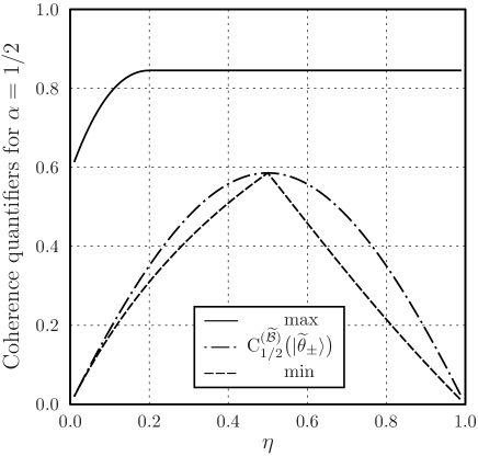
Figure 1: Coherence $\alpha$-quantifiers for $\alpha=1/2$ versus $\eta\in(0;1)$.

The value $\alpha=2$ leads to another relatively simple choice. It turns out that the $2$-quantifier coincides here with the $\ell_{1}$-norm of coherence. For a pure state, the logarithmic coherence of apwl17 can be interpreted in terms of the Rényi entropy of certain order. Our approach leads to another entropy-based reformulation of the $\ell_{1}$-norm of coherence. In the case of pure states, one has

$${\mathrm{C}}_{2}^{(\widetilde{\mathcal{B}})}(|\widetilde{\psi}\rangle)=(\sqrt{p_{+}}+\sqrt{p_{-}}+\sqrt{p_{?}})^{2}-1$$

$$=2\sqrt{p_{+}p_{-}}+2\sqrt{p_{-}p_{?}}+2\sqrt{p_{?}p_{+}}={\mathrm{C}}_{\ell_{1}}^{(\widetilde{\mathcal{B}})}(|\widetilde{\psi}\rangle)\,.$$ (91)

It follows from $p_{+}+p_{-}=1-z$ and (86) that

$$2\sqrt{p_{+}p_{-}}=\sqrt{(1-z)^{2}+2y^{2}}=\frac{|\eta-z|}{\eta}.$$ (92)

Taking $z\in[0;2b]$, we wish to minimize the sum of square roots of the three probabilities. Due to (92), this sum appears as

$$f(z)=\sqrt{p_{+}}+\sqrt{p_{-}}+\sqrt{p_{?}}=\sqrt{1-z+\eta^{-1}|\eta-z|}+\sqrt{z}\,.$$ (93)

For $0\leq{z}\leq\eta$, we deal with the concave function $\sqrt{2-z/b}+\sqrt{z}$. Its minimal value is one of two least values $f(0)=\sqrt{2}$ and $f(\eta)=\sqrt{1-\eta}+\sqrt{\eta}$. Except for $\eta=1/2$, the term $f(\eta)$ is strictly less than $f(0)$. For $\eta\leq{z}\leq 2b$, our concave function is written as

$$\sqrt{z}\,\sqrt{\frac{1-\eta}{\eta}}+\sqrt{z}\,.$$ (94)

Here, we have $f(\eta)=\sqrt{1-\eta}+\sqrt{\eta}$ again and $f(2b)=f(\eta)\sqrt{2/(1+\eta)}$. To sum up, we conclude that

$$\min{\mathrm{C}}_{2}^{(\widetilde{\mathcal{B}})}(|\widetilde{\psi}\rangle)=\sqrt{1-\eta}+\sqrt{\eta}={\mathrm{C}}_{2}^{(\widetilde{\mathcal{B}})}(|\widetilde{\theta}_{\pm}\rangle)\,.$$ (95)

That is, the states $|\widetilde{\theta}_{\pm}\rangle$ to be discriminated minimize the coherence $2$-quantifier exactly. In view of (91), the same conclusion holds for the $\ell_{1}$-norm of coherence. In figure 2, we show the maximal and minimal values of ${\mathrm{C}}_{2}^{(\widetilde{\mathcal{B}})}(|\widetilde{\psi}\rangle)$ as functions of the parameter $\eta$. Overall, the picture is similar to that is related to the case $\alpha=1/2$. The only distinction is that the states $|\widetilde{\theta}_{\pm}\rangle$ exactly minimize the quantifier for $\alpha=2$.

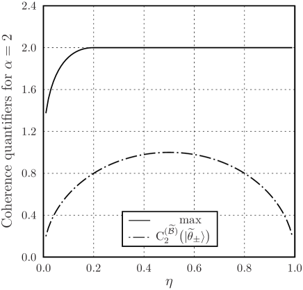
Figure 2: Coherence $\alpha$-quantifiers for $\alpha=2$ versus $\eta\in(0;1)$. The curve ${\mathrm{C}}_{2}^{(\widetilde{\mathcal{B}})}(|\widetilde{\theta}_{\pm}\rangle)$ also gives the minimal value.

To complete the discussion, we also consider the value $\alpha=1$. For pure states, the corresponding measure of coherence appears as the Shannon entropy of generated probability distribution. For $|\widetilde{\theta}_{\pm}\rangle$, we obtain the binary Shannon entropy

$${\mathrm{C}}_{1}^{(\widetilde{\mathcal{B}})}(|\widetilde{\theta}_{\pm}\rangle)=h_{1}(\eta)=\!{}-(1-\eta)\ln(1-\eta)-\eta\ln\eta\,.$$ (96)

The minimization is difficult to formulate analytically. Nevertheless, we can present the results of numerical investigation. In figure 3, we draw the maximal and minimal values of ${\mathrm{C}}_{1}^{(\widetilde{\mathcal{B}})}\bigl{(}|\widetilde{\psi}\rangle\bigr{)}$ together with (96) as functions of the parameter $\eta$. Similarly to figure 1, the states $|\widetilde{\theta}_{\pm}\rangle$ give almost minimal values.

Figure 3: Coherence $\alpha$-quantifiers for $\alpha=1$ versus $\eta\in(0;1)$.

We have studied characteristics of coherence losses during unambiguous state discrimination. Various coherence quantifiers were actually connected with the extended space $\widetilde{\mathcal{H}}=\mathcal{H}\oplus\mathcal{H}^{\prime}$. On the other hand, the states under consideration have non-zero components only in the principal space $\mathcal{H}$. For pure states, the maximum of the coherence $\alpha$-quantifier as a function of $\eta$ is expressed by (82) and (83). To study minimal values, we choose the $\alpha$-quantifiers for $\alpha=1/2,1,2$. Due to (91), our choice includes the $\ell_{1}$-norm of coherence as well. The measurement for unambiguous state discrimination is designed to distinguish states $|\theta_{+}\rangle$ and $|\theta_{-}\rangle$ without the error of mis-identification. For these states, visible losses of quantum coherence are minimal or almost minimal.

V Conclusions

We have considered some coherence quantifiers from the viewpoint of their changes in quantum measurements. For an observable with possibly degenerate eigenvalues, there exist two different ways to formulate the state immediately following a measurement. These ways are commonly referred as the von Neumann and Lüders reduction rules. The latter implies the quantum operation written in terms of the corresponding projectors. Due to another choice of incoherent states, coherence quantifiers are defined via optimization over a larger set of allowed states. We applied this approach to quantities based on quantum $\alpha$-divergences of the Tsallis type. It was shown that such coherence quantifiers succeed the same formal properties as defined with respect to an orthonormal bases. The robustness of coherence and the coherence weight have also been addressed briefly. To illustrate distinctions between the Lüders and von Neumann pictures in the sense of coherence losses, we considered an example of some spin observable with a degenerate eigenvalue. Different coherence measures lead to similar conclusions about the level of residual coherence.

Another interesting question concerns ways to characterize decreases of quantum coherence in POVM measurements. We focused on rank-one POVMs, since they just include principal features of the problem. In this case, we finally deal with some orthonormal basis in the extended space. Hence, basic ways to quantifying the amount of quantum coherence can be applied. Of course, the construction described contains a unitary freedom. Since the $\ell_{1}$-norm of coherence and coherence $\alpha$-quantifiers are expressed via matrix elements of the density matrix and its powers, they are independent of this freedom. The proposed approach is exemplified using a POVM designed for unambiguous discrimination of two non-orthogonal pure states. It can naturally be converted into orthonormal basis in the three-dimensional space. Taking arbitrary pure state, we study the maximal and minimal values of the chosen quantifiers as function of the overlap between two states to be identified. In the sense of coherence losses, these two states clearly reveal some extreme properties.

References

- (1) Deutsch D (1985) Proc. R. Soc. Lond. A 400 97
- (2) Zurek W H (1981) Phys. Rev. D 24 1516
- (3) Ćwikliński P, Studziński M, Horodecki M and Oppenheim J (2015) Phys. Rev. Lett. 115 210403
- (4) Narasimhachar V and Gour G (2015) Nat. Commun. 6 7689
- (5) Adesso G, Bromley T R and Cianciaruso M (2016) J. Phys. A: Math. Theor. 49 473001
- (6) Hu M-L, Hu X, Wang J-C, Peng Y, Zhang Y-R and Fan H (2017) Quantum coherence and quantum correlations (arXiv:1703.01852)
- (7) Yao Yao, Dong G H, Xing Xiao, Mo Li and Sun C P (2017) Phys. Rev. A 96 052322
- (8) von Neumann J (1932) Mathematische Grundlagen der Quantenmechanik (Berlin: Springer)
- (9) Lüders G (1950) Ann. Phys. (Leipzig) 443 322
- (10) Baumgratz T, Cramer M and Plenio M B (2014) Phys. Rev. Lett. 113 140401
- (11) Napoli C, Bromley T R, Cianciaruso M, Piani M, Johnston N and Adesso G (2016) Phys. Rev. Lett. 116 150502
- (12) Bu K, Anand N and Singh U (2017) Asymmetry and coherence weight of quantum states (arXiv:1703.01266)
- (13) Yao Yao, Dong G H, Li Ge, Mo Li and Sun C P (2016) Phys. Rev. A 94 062339
- (14) Hu M-L, Shen S-Q and Fan H (2017) Phys. Rev. A 96 052309
- (15) Horn R A and Johnson C R (1985) Matrix Analysis (Cambridge: Cambridge University Press)
-
(16)
Watrous J (2018) Theory of Quantum Information (Waterloo: University of Waterloo)
http://cs.uwaterloo.ca/~watrous/TQI/ - (17) Nielsen M A and Chuang I L (2000) Quantum Computation and Quantum Information (Cambridge: Cambridge University Press)
- (18) Vedral V (2002) Rev. Mod. Phys. 74 197
- (19) Hiai F, Mosonyi M, Petz D and Bény C (2011) Rev. Math. Phys. 23 691
- (20) Bengtsson I and Życzkowski K (2006) Geometry of Quantum States: An Introduction to Quantum Entanglement (Cambridge: Cambridge University Press)
- (21) Csiszár I (2008) Entropy 10 261
- (22) Borland L, Plastino A R and Tsallis C (1998) J. Math. Phys. 39 6490
- (23) Furuichi S, Yanagi K and Kuriyama K (2004) J. Math. Phys. 45 4868
- (24) Liese F and Vajda I (2006) IEEE Trans. Inf. Theor. 52 4394
- (25) Csiszár I (1967) Studia Sci. Math. Hungar. 2 299
- (26) Marvian I and Spekkens R (2013) New J. Phys. 15 033001
- (27) Piani M, Cianciaruso M, Bromley T R, Napoli C, Johnston N and Adesso G (2016) Phys. Rev. A 93 042107
- (28) Hegerfeldt G C and Sala Mayato R (2012) Phys. Rev. A 85 032116
- (29) Sala Mayato R and Muga J G (2011) Phys. Lett. A 375 3167
- (30) Sudheer Kumar C S, Abhishek Shukla and Mahesh T S (2016) Phys. Lett. A 380 3612
- (31) Davies E B (1978) IEEE Trans. Inf. Theory 24 596
- (32) Marvian I and Spekkens R W (2016) Phys. Rev. A 94 052324
- (33) Chitambar E and Gour G (2016) Phys. Rev. A 94 052336
- (34) Streltsov A, Adesso G and Plenio M B (2017) Rev. Mod. Phys. 89 041003
- (35) Bera M N, Qureshi T, Siddiqui M A and Pati A K (2015) Phys. Rev. A 92 012118
- (36) Bagan E, Bergou J A, Cottrell S S and Hillery M (2016) Phys. Rev. Lett. 116 160406
- (37) Qureshi T and Siddiqui M A (2017) Ann. Phys. 385 598
- (38) Rana S, Parashar P, Winter A and Lewenstein M (2017) Phys. Rev. A 96 052336
- (39) Cheng S and Hall M J W (2015) Phys. Rev. A 92 042101
- (40) Peng Y, Zhang Y-R, Fan Z-Y, Liu S and Fan H (2016) Complementary relation of quantum coherence and quantum correlations in multiple measurements (arXiv:1608.07950)
- (41) Singh U, Pati A K and Bera M N (2016) Mathematics 4 47
- (42) Yuan X, Bai G, Peng T and Ma X (2017) Phys. Rev. A 96 032313
- (43) Rastegin A E (2018) Front. Phys. 13 130304
- (44) Rastegin A E (2016) Phys. Rev. A 93 032136
-
(45)
Preskill J (2018) Quantum Computation (Pasadena: California Institute of Technology)
http://www.theory.caltech.edu/people/preskill/ph229/ - (46) Brandt H E (2005) Quantum Inf. Process. 4 387
- (47) Shapiro J H (2006) Quantum Inf. Process. 5 11
- (48) Rastegin A E (2016) Quantum Inf. Process. 15 1225
- (49) Rockafellar R T (1970) Convex Analysis (Princeton: Princeton University Press)