Undecidability of future timeline-based planning
over dense temporal domains

Abstract

Planning is one of the most studied problems in computer science. In this paper, we consider the timeline-based approach, where the domain is modeled by a set of independent, but interacting, components, identified by a set of state variables, whose behavior over time (timelines) is governed by a set of temporal constraints (synchronization rules). Timeline-based planning in the dense-time setting has been recently shown to be undecidable in the general case, and undecidability relies on the high expressiveness of the trigger synchronization rules. In this paper, we strengthen the previous negative result by showing that undecidability already holds under the future semantics of the trigger rules which limits the comparison to temporal contexts in the future with respect to the trigger.

1 Introduction

Timeline-based planning (TP for short) represents a promising approach for real-time temporal planning and reasoning about execution under uncertainty [15, 13, 14, 9, 10, 12]. Compared to classical action-based temporal planning [16, 25], TP adopts a more declarative paradigm which is focused on the constraints that sequences of actions have to fulfill to reach a fixed goal. In TP, the planning domain is modeled as a set of independent, but interacting, components, each one identified by a state variable. The temporal behaviour of a single state variable (component) is described by a sequence of tokens (timeline) where each token specifies a value of variable (state) and the period of time during which the variable assumes that value. The overall temporal behaviour (set of timelines) is constrained by a set of synchronization rules which specify quantitative temporal requirements between the time events (start-time and end-time) of distinct tokens. Synchronization rules have a very simple format: either trigger rules expressing invariants and response properties (for each token with a fixed state, called trigger, there exist tokens satisfying some mutual temporal relations) or trigger-less rules expressing goals (there exist tokens satisfying some mutual temporal relations). Note that the way in which timing requirements are specified in the synchronization rules corresponds to the “freeze” mechanism in the well-known timed temporal logic TPTL [3] which uses the freeze quantifier to bind a variable to a specific temporal context (a token in the TP setting).

TP has been successfully exploited in a number of application domains, including space missions, constraint solving, and activity scheduling (see, e.g., [22, 20, 17, 8, 11, 5]). A systematic study of expressiveness and complexity issues for TP has been undertaken only very recently both in the discrete-time and dense-time settings [18, 19, 7, 6]. In the discrete-time context, the TP problem is $\operatorname{\mathbf{EXPSPACE}}$-complete, and is expressive enough to capture action-based temporal planning (see [18, 19]).

On the other hand, despite the simple format of synchronization rules, the shift to a dense-time domain dramatically increases expressiveness, depicting a scenario which resembles that of the well-known timed linear temporal logics MTL and TPTL (under a pointwise semantics) which are undecidable in the general setting [3, 23]. In fact the TP problem is undecidable in the general case [7], and undecidability relies on the high expressiveness of the trigger rules (by restricting the formalism to only trigger-less rules the problem is just $\operatorname{\mathbf{NP}}$-complete [7]). Decidability can be recovered by suitable (syntactic/semantic) restrictions on the trigger rules. In particular, in [6], two restrictions are considered: (i) the first one limits the comparison to tokens whose start times follow the trigger start time (future semantics of trigger rules), and (ii) the second one is syntactical and imposes that a non-trigger token can be referenced at most once in the timed constraints of a trigger rule (simple trigger rules). Note that the second restriction avoids comparisons of multiple token time-events with a non-trigger reference time-event. Under the previous two restrictions, the TP problem is decidable with a non-primitive recursive complexity [6] and can be solved by a reduction to model checking of Timed Automata(TA) [4] against MTL over finite timed words, the latter being a known decidable problem [24]. As in the case of MTL [2], better complexity results, i.e. $\operatorname{\mathbf{EXPSPACE}}$-completeness (resp., $\operatorname{\mathbf{PSPACE}}$-completeness) can be obtained by restricting also the type of intervals used in the simple trigger rules in order to compare tokens: non-singular intervals (resp., intervals unbounded or starting from $0$).

In this paper, we show that both the considered restrictions on the trigger rules are necessary to recovery decidability. The undecidability of the TP problem with simple trigger rules has been already established in [7]. Here, we prove undecidability of the TP problem with arbitrary trigger rules under the future semantics.

2 Preliminaries

Let $\mathbb{N}$ be the set of natural numbers, ${\mathbb{R}_{+}}$ be the set of non-negative real numbers, and ${\mathit{Intv}}$ be the set of intervals in ${\mathbb{R}_{+}}$ whose endpoints are in $\mathbb{N}\cup\{\infty\}$. Moreover, let us denote by ${\mathit{Intv}}_{(0,\infty)}$ the set of intervals $I\in{\mathit{Intv}}$ such that either $I$ is unbounded, or $I$ is left-closed with left endpoint $0$. Such intervals $I$ can be replaced by expressions of the form $\sim n$ for some $n\in\mathbb{N}$ and $\sim\in\{<,\leq,>,\geq\}$. Let $w$ be a finite word over some alphabet. By $|w|$ we denote the length of $w$. For all $0\leq i<|w|$, $w(i)$ is the $i$-th letter of $w$.

2.1 The TP Problem

In this section, we recall the TP framework as presented in [14, 18]. In TP, domain knowledge is encoded by a set of state variables, whose behaviour over time is described by transition functions and synchronization rules.

Definition 1.

A state variable $x$ is a triple $x=(V_{x},T_{x},D_{x})$, where $V_{x}$ is the finite domain of the variable $x$, $T_{x}:V_{x}\to 2^{V_{x}}$ is the value transition function, which maps each $v\in V_{x}$ to the (possibly empty) set of successor values, and $D_{x}:V_{x}\to{\mathit{Intv}}$ is the constraint function that maps each $v\in V_{x}$ to an interval.

A token for a variable $x$ is a pair $(v,d)$ consisting of a value $v\in V_{x}$ and a duration $d\in{\mathbb{R}_{+}}$ such that $d\in D_{x}(v)$. Intuitively, a token for $x$ represents an interval of time where the state variable $x$ takes value $v$. The behavior of the state variable $x$ is specified by means of timelines which are non-empty sequences of tokens $\pi=(v_{0},d_{0})\ldots(v_{n},d_{n})$ consistent with the value transition function $T_{x}$, that is, such that $v_{i+1}\in T_{x}(v_{i})$ for all $0\leq i<n$. The start time $\mathsf{s}(\pi,i)$ and the end time $\mathsf{e}(\pi,i)$ of the $i$-th token ($0\leq i\leq n$) of the timeline $\pi$ are defined as follows: $\mathsf{e}(\pi,i)=\displaystyle{\sum_{h=0}^{i}}d_{h}$ and $\mathsf{s}(\pi,i)=0$ if $i=0$, and $\mathsf{s}(\pi,i)=\displaystyle{\sum_{h=0}^{i-1}}d_{h}$ otherwise. See Figure 1 for an example.

Figure 1: An example of timeline $(a,7)(b,3)(c,3.9)\cdots$ for the state variable $x=(V_{x},T_{x},D_{x})$, where $V_{x}=\{a,b,c,\ldots\}$, $b\in T_{x}(a)$, $c\in T_{x}(b)$, $b\in T_{x}(c)$…and $D_{x}(a)=[5,8]$, $D_{x}(b)=[1,4]$, $D_{x}(c)=[2,\infty[$…

Given a finite set $SV$ of state variables, a multi-timeline of $SV$ is a mapping $\Pi$ assigning to each state variable $x\in SV$ a timeline for $x$. Multi-timelines of $SV$ can be constrained by a set of synchronization rules, which relate tokens, possibly belonging to different timelines, through temporal constraints on the start/end-times of tokens (time-point constraints) and on the difference between start/end-times of tokens (interval constraints). The synchronization rules exploit an alphabet $\Sigma$ of token names to refer to the tokens along a multi-timeline, and are based on the notions of atom and existential statement.

Definition 2.

An atom is either a clause of the form $o_{1}\leq^{e_{1},e_{2}}_{I}o_{2}$ (interval atom), or of the forms $o_{1}\leq^{e_{1}}_{I}n$ or $n\leq^{e_{1}}_{I}o_{1}$ (time-point atom), where $o_{1},o_{2}\in\Sigma$, $I\in{\mathit{Intv}}$, $n\in\mathbb{N}$, and $e_{1},e_{2}\in\{\mathsf{s},\mathsf{e}\}$.

An atom $\rho$ is evaluated with respect to a $\Sigma$-assignment $\lambda_{\Pi}$ for a given multi-timeline $\Pi$ which is a mapping assigning to each token name $o\in\Sigma$ a pair $\lambda_{\Pi}(o)=(\pi,i)$ such that $\pi$ is a timeline of $\Pi$ and $0\leq i<|\pi|$ is a position along $\pi$ (intuitively, $(\pi,i)$ represents the token of $\Pi$ referenced by the name $o$). An interval atom $o_{1}\leq^{e_{1},e_{2}}_{I}o_{2}$ is satisfied by $\lambda_{\Pi}$ if $e_{2}(\lambda_{\Pi}(o_{2}))-e_{1}(\lambda_{\Pi}(o_{1}))\in I$. A point atom $o\leq^{e}_{I}n$ (resp., $n\leq^{e}_{I}o$) is satisfied by $\lambda_{\Pi}$ if $n-e(\lambda_{\Pi}(o))\in I$ (resp., $e(\lambda_{\Pi}(o))-n\in I$).

Definition 3.

An existential statement $\mathcal{E}$ for a finite set $SV$ of state variables is a statement of the form:

$$\mathcal{E}:=\exists o_{1}[x_{1}=v_{1}]\cdots\exists o_{n}[x_{n}=v_{n}].\mathcal{C}$$

where $\mathcal{C}$ is a conjunction of atoms, $o_{i}\in\Sigma$, $x_{i}\in SV$, and $v_{i}\in V_{x_{i}}$ for each $i=1,\ldots,n$. The elements $o_{i}[x_{i}=v_{i}]$ are called quantifiers. A token name used in $\mathcal{C}$, but not occurring in any quantifier, is said to be free. Given a $\Sigma$-assignment $\lambda_{\Pi}$ for a multi-timeline $\Pi$ of $SV$, we say that $\lambda_{\Pi}$ is consistent with the existential statement $\mathcal{E}$ if for each quantified token name $o_{i}$, $\lambda_{\Pi}(o_{i})=(\pi,h)$ where $\pi=\Pi(x_{i})$ and the $h$-th token of $\pi$ has value $v_{i}$. A multi-timeline $\Pi$ of $SV$ satisfies $\mathcal{E}$ if there exists a $\Sigma$-assignment $\lambda_{\Pi}$ for $\Pi$ consistent with $\mathcal{E}$ such that each atom in $\mathcal{C}$ is satisfied by $\lambda_{\Pi}$.

Definition 4.

A synchronization rule $\mathcal{R}$ for a finite set $SV$ of state variables is a rule of one of the forms

$$o_{0}[x_{0}=v_{0}]\to\mathcal{E}_{1}\lor\mathcal{E}_{2}\lor\ldots\lor\mathcal{E}_{k},\quad\top\to\mathcal{E}_{1}\lor\mathcal{E}_{2}\lor\ldots\lor\mathcal{E}_{k},$$

where $o_{0}\in\Sigma$, $x_{0}\in SV$, $v_{0}\in V_{x_{0}}$, and $\mathcal{E}_{1},\ldots,\mathcal{E}_{k}$ are existential statements. In rules of the first form (trigger rules), the quantifier $o_{0}[x_{0}=v_{0}]$ is called trigger, and we require that only $o_{0}$ may appear free in $\mathcal{E}_{i}$ (for $i=1,\ldots,n$). In rules of the second form (trigger-less rules), we require that no token name appears free.

Intuitively, a trigger $o_{0}[x_{0}=v_{0}]$ acts as a universal quantifier, which states that for all the tokens of the timeline for the state variable $x_{0}$, where the variable $x_{0}$ takes the value $v_{0}$, at least one of the existential statements $\mathcal{E}_{i}$ must be true. Trigger-less rules simply assert the satisfaction of some existential statement. The semantics of synchronization rules is formally defined as follows.

Definition 5.

Let $\Pi$ be a multi-timeline of a set $SV$ of state variables. Given a trigger-less rule $\mathcal{R}$ of $SV$, $\Pi$ satisfies $\mathcal{R}$ if $\Pi$ satisfies some existential statement of $\mathcal{R}$. Given a trigger rule $\mathcal{R}$ of $SV$ with trigger $o_{0}[x_{0}=v_{0}]$, $\Pi$ satisfies $\mathcal{R}$ if for every position $i$ of the timeline $\Pi(x_{0})$ for $x_{0}$ such that $\Pi(x_{0})=(v_{0},d)$, there is an existential statement $\mathcal{E}$ of $\mathcal{R}$ and a $\Sigma$-assignment $\lambda_{\Pi}$ for $\Pi$ which is consistent with $\mathcal{E}$ such that $\lambda_{\Pi}(o_{0})=(\Pi(x_{0}),i)$ and $\lambda_{\Pi}$ satisfies all the atoms of $\mathcal{E}$.

In the paper, we focus on a stronger notion of satisfaction of trigger rules, called satisfaction under the future semantics. It requires that all the non-trigger selected tokens do not start strictly before the start-time of the trigger token.

Definition 6.

A multi-timeline $\Pi$ of $SV$ satisfies under the future semantics a trigger rule $\mathcal{R}=o_{0}[x_{0}=v_{0}]\to\mathcal{E}_{1}\vee\mathcal{E}_{2}\vee\ldots\vee\mathcal{E}_{k}$ if $\Pi$ satisfies the trigger rule obtained from $\mathcal{R}$ by replacing each existential statement $\mathcal{E}_{i}=\exists o_{1}[x_{1}=v_{1}]\cdots\exists o_{n}[x_{n}=v_{n}].\mathcal{C}$ with $\exists o_{1}[x_{1}=v_{1}]\cdots\exists o_{n}[x_{n}=v_{n}].\mathcal{C}\wedge\bigwedge_{i=1}^{n}o_{0}\leq^{\mathsf{s},\mathsf{s}}_{[0,+\infty[}o_{i}$.

A TP domain $P=(SV,R)$ is specified by a finite set $SV$ of state variables and a finite set $R$ of synchronization rules modeling their admissible behaviors. Trigger-less rules can be used to express initial conditions and the goals of the problem, while trigger rules are useful to specify invariants and response requirements. A plan of $P$ is a multi-timeline of $SV$ satisfying all the rules in $R$. A future plan of $P$ is defined in a similar way, but we require that the fulfillment of the trigger rules is under the future semantics. We are interested in the Future TP problem consisting in checking for a given TP domain $P=(SV,R)$, the existence of a future plan for $P$.

3 Undecidability of the future TP problem

In this section, we establish the following result.

Theorem 7.

Future TP with one state variable is undecidable even if the intervals are in ${\mathit{Intv}}_{(0,\infty)}$.

Theorem 7 is proved by a polynomial-time reduction from the halting problem for Minsky $2$-counter machines [21]. Such a machine is a tuple $M=(Q,q_{\textit{init}},q_{\textit{halt}},\Delta)$, where $Q$ is a finite set of (control) locations, $q_{\textit{init}}\in Q$ is the initial location, $q_{\textit{halt}}\in Q$ is the halting location, and $\Delta\subseteq Q\times{\textit{L}}\times Q$ is a transition relation over the instruction set ${\textit{L}}=\{{\mathsf{inc}},{\mathsf{dec}},{\mathsf{zero}}\}\times\{1,2\}$.

We adopt the following notational conventions. For an instruction ${\textit{op}}=(\_\,,c)\in{\textit{L}}$, let $c({\textit{op}}):=c\in\{1,2\}$ be the counter associated with op. For a transition $\delta\in\Delta$ of the form $\delta=(q,{\textit{op}},q^{\prime})$, we define ${\textit{from}}(\delta):=q$, ${\textit{op}}(\delta):={\textit{op}}$, $c(\delta):=c({\textit{op}})$, and ${\textit{to}}(\delta):=q^{\prime}$. Without loss of generality, we make these assumptions:

• for each transition $\delta\in\Delta$, ${\textit{from}}(\delta)\neq q_{\textit{halt}}$ and ${\textit{to}}(\delta)\neq q_{\textit{init}}$, and

• there is exactly one transition in $\Delta$, denoted $\delta_{\textit{init}}$, having as source the initial location $q_{\textit{init}}$.

An $M$-configuration is a pair $(q,\nu)$ consisting of a location $q\in Q$ and a counter valuation $\nu:\{1,2\}\to\mathbb{N}$. $M$ induces a transition relation, denoted by $\longrightarrow$, over pairs of $M$-configurations defined as follows. For configurations $(q,\nu)$ and $(q^{\prime},\nu^{\prime})$, $(q,\nu)\;\;{\mathop{{\longrightarrow}}\limits}\!\;\;(q^{\prime},\nu^{\prime})$ if for some instruction ${\textit{op}}\in{\textit{L}}$, $(q,{\textit{op}},q^{\prime})\in\Delta$ and the following holds, where $c\in\{1,2\}$ is the counter associated with the instruction op: (i) $\nu^{\prime}(c^{\prime})=\nu(c^{\prime})$if $c^{\prime}\neq c$; (ii) $\nu^{\prime}(c)=\nu(c)+1$if ${\textit{op}}=({\mathsf{inc}},c)$; (iii) $\nu(c)>0$and $\nu^{\prime}(c)=\nu(c)-1$ if ${\textit{op}}=({\mathsf{dec}},c)$; and (iv) $\nu^{\prime}(c)=\nu(c)=0$if ${\textit{op}}=({\mathsf{zero}},c)$.

A computation of $M$ is a non-empty finite sequence $C_{1},\ldots,C_{k}$ of configurations such that $C_{i}\;\;{\mathop{{\longrightarrow}}\limits}\!\;\;C_{i+1}$ for all $1\leq i<k$. $M$ halts if there is a computation starting at the initial configuration $(q_{\textit{init}},\nu_{\textit{init}})$, where $\nu_{\textit{init}}(1)=\nu_{\textit{init}}(2)=0$, and leading to some halting configuration $(q_{{\textit{halt}}},\nu)$. The halting problem is to decide whether a given machine $M$ halts, and it is was proved to be undecidable [21]. We prove the following result, from which Theorem 7 directly follows.

Proposition 8.

One can construct (in polynomial time) a TP instance (domain) $P=(\{x_{M}\},R_{M})$ where the intervals in $P$ are in ${\mathit{Intv}}_{(0,\infty)}$ such that $M$ halts iff there exists a future plan for $P$.

Proof.

First, we define a suitable encoding of a computation of $M$ as the untimed part of a timeline (i.e., neglecting tokens’ durations and accounting only for their values) for $x_{M}$. For this, we exploit the finite set of symbols $V:=V_{{\textit{main}}}\cup V_{{\textit{sec}}}$ corresponding to the finite domain of the state variable $x_{M}$. The set of main values $V_{{\textit{main}}}$ is the set of $M$-transitions, i.e. $V_{{\textit{main}}}=\Delta$. The set of secondary values $V_{{\textit{sec}}}$ is defined as $V_{\textit{sec}}:=\Delta\times\{1,2\}\times\{\#,\textit{beg},\textit{end}\}$, where $\#$, beg, and end are three special symbols used as markers. Intuitively, in the encoding of an $M$-computation a main value keeps track of the transition used in the current step of the computation, while the set $V_{{\textit{sec}}}$ is used for encoding counter values.

For $c\in\{1,2\}$, a $c$-code for the main value $\delta\in\Delta$ is a finite word $w_{c}$ over $V_{\textit{sec}}$ of the form $(\delta,c,\textit{beg})\cdot(\delta,c,\#)^{h}\cdot(\delta,c,\textit{end})$ for some $h\geq 0$ such that $h=0$ if ${\textit{op}}(\delta)=({\mathsf{zero}},c)$. The $c$-code $w_{c}$ encodes the value for counter $c$ given by $h$ (or equivalently $|w_{c}|-2$). Note that only the occurrences of the symbols $(\delta,c,\#)$ encode units in the value of counter $c$, while the symbol $(\delta,c,\textit{beg})$ (resp., $(\delta,c,\textit{end})$) is only used as left (resp., right) marker in the encoding.

A configuration-code $w$ for a main value $\delta\in\Delta$ is a finite word over $V$ of the form $w=\delta\cdot w_{1}\cdot w_{2}$ such that for each counter $c\in\{1,2\}$, $w_{c}$ is a $c$-code for the main value $\delta$. The configuration-code $w$ encodes the $M$-configuration $({\textit{from}}(\delta),\nu)$, where $\nu(c)=|w_{c}|-2$ for all $c\in\{1,2\}$. Note that if ${\textit{op}}(\delta)=({\mathsf{zero}},c)$, then $\nu(c)=0$.

A computation-code is a non-empty sequence of configuration-codes $\pi=w_{\delta_{1}}\cdots w_{\delta_{k}}$, where for all $1\leq i\leq k$, $w_{\delta_{i}}$ is a configuration-code with main value $\delta_{i}$, and whenever $i<k$, it holds that ${\textit{to}}(\delta_{i})={\textit{from}}(\delta_{i+1})$. Note that by our assumptions ${\textit{to}}(\delta_{i})\neq q_{\textit{halt}}$ for all $1\leq i<k$, and $\delta_{j}\neq\delta_{\textit{init}}$ for all $1<j\leq k$. The computation-code $\pi$ is initial if the first configuration-code $w_{\delta_{1}}$ has the main value $\delta_{\textit{init}}$ and encodes the initial configuration, and it is halting if for the last configuration-code $w_{\delta_{k}}$ in $\pi$, it holds that ${\textit{to}}(\delta_{k})=q_{\textit{halt}}$. For all $1\leq i\leq k$, let $(q_{i},\nu_{i})$ be the $M$-configuration encoded by the configuration-code $w_{\delta_{i}}$ and $c_{i}=c(\delta_{i})$. The computation-code $\pi$ is well-formed if, additionally, for all $1\leq j<k$, the following holds:

• $\nu_{j+1}(c)=\nu_{j}(c)$ if either $c\neq c_{j}$ or ${\textit{op}}(\delta_{j})=({\mathsf{zero}},c_{j})$ (equality requirement);

• $\nu_{j+1}(c_{j})=\nu_{j}(c_{j})+1$ if ${\textit{op}}(\delta_{j})=({\mathsf{inc}},c_{j})$ (increment requirement);

• $\nu_{j+1}(c_{j})=\nu_{j}(c_{j})-1$ if ${\textit{op}}(\delta_{j})=({\mathsf{dec}},c_{j})$ (decrement requirement).

Clearly, $M$ halts iff there exists an initial and halting well-formed computation-code.

Definition of $x_{M}$ and $R_{M}$.

We now define a state variable $x_{M}$ and a set $R_{M}$ of synchronization rules for $x_{M}$ with intervals in ${\mathit{Intv}}_{(0,\infty)}$ such that the untimed part of every future plan of $P=(\{x_{M}\},R_{M})$ is an initial and halting well-formed computation-code. Thus, $M$ halts iff there is a future plan of $P$.

Formally, variable $x_{M}$ is given by $x_{M}=(V=V_{{\textit{main}}}\cup V_{{\textit{sec}}},T,D)$, where for each $v\in V$, $D(v)=]0,\infty[$. Thus, we require that the duration of a token is always greater than zero (strict time monotonicity). The value transition function $T$ of $x_{M}$ ensures the following property.

Claim 9.

The untimed parts of the timelines for $x_{M}$ whose first token has value $\delta_{\textit{init}}$ correspond to the prefixes of initial computation-codes. Moreover, $\delta_{\textit{init}}\notin T(v)$ for all $v\in V$.

By construction, it is a trivial task to define $T$ so that the previous requirement is fulfilled.

Let $V_{\textit{halt}}=\{\delta\in\Delta\mid{\textit{to}}(\delta)=q_{\textit{halt}}\}$. By Claim 9 and the assumption that ${\textit{from}}(\delta)\neq q_{\textit{halt}}$ for each transition $\delta\in\Delta$, in order to enforce the initialization and halting requirements, it suffices to ensure that a timeline has a token with value $\delta_{\textit{init}}$ and a token with value in $V_{\textit{halt}}$. This is captured by the trigger-less rules $\top\rightarrow\exists o[x_{M}=\delta_{\textit{init}}].\top$ and $\top\rightarrow\bigvee_{v\in V_{\textit{halt}}}\exists o[x_{M}=v].\top$.

Finally, the crucial well-formedness requirement is captured by the trigger rules in $R_{M}$ which express punctual time constraints. We refer the reader to Figure 2, that gives an intuition on the properties enforced by the rules we are about to define. In particular, we essentially take advantage of the dense temporal domain to allow for the encoding of arbitrarily large values of counters in one time units.

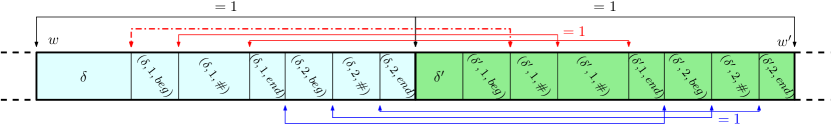
Figure 2: The figure shows two adjacent configuration-codes, $w$ (highlighted in cyan) and $w^{\prime}$ (in green), the former for $\delta=(q,(\mathsf{inc},1),q^{\prime})\in\Delta$ and the latter for $\delta^{\prime}=(q^{\prime},\dots)\in\Delta$; $w$ encodes the $M$-configuration $(q,\nu)$ where $\nu(1)=\nu(2)=1$, and $w^{\prime}$ the $M$-configuration $(q^{\prime},\nu^{\prime})$ where $\nu^{\prime}(1)=2$ and $\nu^{\prime}(1)=1$.
The “1-Time distance between consecutive main values requirement” (represented by black lines with arrows) forces a token with a main value to be followed, after exactly one time instant, by another token with a main value.
Since ${\textit{op}}(\delta)=({\mathsf{inc}},1)$, the value of counter 2 does not change in this computation step, and thus the values for counter 2 encoded by $w$ and $w^{\prime}$ must be equal. To this aim the “equality requirement” (represented by blue lines with arrows) sets a one-to-one correspondence between pairs of tokens associated with counter 2 in $w$ and $w^{\prime}$ (more precisely, a token $tk$ with value $(\delta,2,\_)$ in $w$ is followed by a token $tk^{\prime}$ with value $(\delta^{\prime},2,\_)$ in $w^{\prime}$ such that $\mathsf{s}(tk^{\prime})-\mathsf{s}(tk)=1$ and $\mathsf{e}(tk^{\prime})-\mathsf{e}(tk)=1$).
Finally, the “increment requirement” (red lines) performs the increment of counter 1 by doing something analogous to the previous case, but with a difference: the token $tk^{\prime}$ with value $(\delta^{\prime},1,\#)$ is in $w^{\prime}$ in the place where the token $tk$ with value $(\delta,1,\textit{beg})$ was in $w$ (i.e., $\mathsf{s}(tk^{\prime})-\mathsf{s}(tk)=1$ and $\mathsf{e}(tk^{\prime})-\mathsf{e}(tk)=1$). The token $tk^{\prime\prime}$ with value $(\delta^{\prime},1,\textit{beg})$ is “anticipated”, in such a way that $\mathsf{e}(tk^{\prime\prime})-\mathsf{s}(tk)=1$ (this is denoted by the dashed red line): the token with main value $\delta^{\prime}$ in $w^{\prime}$ has a shorter duration than that with value $\delta$ in $w$, leaving space for $tk^{\prime\prime}$, so as to represent the unit added by $\delta$ to counter 1. Clearly density of the time domain plays a fundamental role here.

Trigger rules for 1-Time distance between consecutive main values.

We define non-simple trigger rules requiring that the overall duration of the sequence of tokens corresponding to a configuration-code amounts exactly to one time units. By Claim 9, strict time monotonicity, and the halting requirement, it suffices to ensure that each token $tk$ having a main value in $V_{\textit{main}}\setminus V_{\textit{halt}}$ is eventually followed by a token $tk^{\prime}$ such that $tk^{\prime}$ has a main value and $\mathsf{s}(tk^{\prime})-\mathsf{s}(tk)=1$ (this denotes—with a little abuse of notation—that the difference of start times is exactly $1$). To this aim, for each $v\in V_{\textit{main}}\setminus V_{\textit{halt}}$, we write the non-simple trigger rule with intervals in ${\mathit{Intv}}_{(0,\infty)}$:

$$o[x_{M}=v]\rightarrow\bigvee_{u\in V_{\textit{main}}}\exists o^{\prime}[x_{M}=u].\,o\leq^{\mathsf{s},\mathsf{s}}_{[1,+\infty[}o^{\prime}\,\wedge\,o\leq^{\mathsf{s},\mathsf{s}}_{[0,1]}o^{\prime}.$$

Trigger rules for the equality requirement.

In order to ensure the equality requirement, we exploit the fact that the end time of a token along a timeline corresponds to the start time of the next token (if any). Let $V_{\textit{sec}}^{=}$ be the set of secondary states $(\delta,c,t)\in V_{\textit{sec}}$ such that ${\textit{to}}(\delta)\neq q_{\textit{halt}}$, and either $c\neq c(\delta)$ or ${\textit{op}}(\delta)=({\mathsf{zero}},c)$. Moreover, for a counter $c\in\{1,2\}$ and a tag $t\in\{\textit{beg},\#,\textit{end}\}$, let $V_{c}^{t}\subseteq V_{\textit{sec}}$ be the set of secondary states given by $\Delta\times\{c\}\times\{t\}$. We require the following:

1. each token $tk$ with a $(V_{c}^{t}\cap V_{\textit{sec}}^{=})$-value is eventually followed by a token $tk^{\prime}$ with a $V_{c}^{t}$-value such that $\mathsf{s}(tk^{\prime})-\mathsf{s}(tk)=1$ (i.e., the difference of start times is exactly $1$). Moreover, if $t\neq\textit{end}$, then $\mathsf{e}(tk^{\prime})-\mathsf{e}(tk)=1$ (i.e., the difference of end times is exactly $1$).

Condition (*) is captured by the following non-simple trigger rules with intervals in ${\mathit{Intv}}_{(0,\infty)}$:

• for each $v\in V^{t}_{c}\cap V_{\textit{sec}}^{=}$ and $t\neq\textit{end}$,

  $$o[x_{M}=v]\rightarrow\bigvee_{u\in V^{t}_{c}}\exists o^{\prime}[x_{M}=u].\,o\leq^{\mathsf{s},\mathsf{s}}_{[1,+\infty[}o^{\prime}\,\wedge\,o\leq^{\mathsf{s},\mathsf{s}}_{[0,1]}o^{\prime}\,\wedge\,o\leq^{\mathsf{e},\mathsf{e}}_{[1,+\infty[}o^{\prime}\,\wedge\,o\leq^{\mathsf{e},\mathsf{e}}_{[0,1]}o^{\prime};$$

• for each $v\in V^{\textit{end}}_{c}\cap V_{\textit{sec}}^{=}$,

  $$o[x_{M}=v]\rightarrow\bigvee_{u\in V^{\textit{end}}_{c}}\exists o^{\prime}[x_{M}=u].\,o\leq^{\mathsf{s},\mathsf{s}}_{[1,+\infty[}o^{\prime}\,\wedge\,o\leq^{\mathsf{s},\mathsf{s}}_{[0,1]}o^{\prime}.$$

We now show that Condition (*) together with strict time monotonicity and 1-Time distance between consecutive main values ensure the equality requirement. Let $\pi$ be a timeline of $x_{M}$ satisfying all the rules defined so far, $w_{\delta}$ and $w_{\delta^{\prime}}$ two adjacent configuration-codes along $\pi$ with $w_{\delta}$ preceding $w_{\delta^{\prime}}$ (note that ${\textit{to}}(\delta)\neq q_{\textit{halt}}$), and $c\in\{1,2\}$ a counter such that either $c\neq c(\delta)$ or ${\textit{op}}(\delta)=({\mathsf{zero}},c)$. Let $tk_{0}\cdots tk_{\ell+1}$ (resp., $tk^{\prime}_{0}\cdots tk^{\prime}_{\ell^{\prime}+1}$) be the sequence of tokens associated with the $c$-code of $w_{\delta}$ (resp., $w_{\delta^{\prime}}$). We need to show that $\ell=\ell^{\prime}$. By construction $tk_{0}$ and $tk^{\prime}_{0}$ have value in $V_{c}^{\textit{beg}}$, $tk_{\ell+1}$ and $tk^{\prime}_{\ell^{\prime}+1}$ have value in $V_{c}^{\textit{end}}$, and for all $1\leq i\leq\ell$ (resp., $1\leq i^{\prime}\leq\ell^{\prime}$), $tk_{i}$ has value in $V_{c}^{\#}$ (resp., $tk^{\prime}_{i^{\prime}}$ has value in $V_{c}^{\#}$). Then strict time monotonicity, 1-Time distance between consecutive main values, and Condition (*) guarantee the existence of an injective mapping $g:\{tk_{0},\ldots,tk_{\ell+1}\}\rightarrow\{tk^{\prime}_{0},\ldots,tk^{\prime}_{\ell^{\prime}+1}\}$ such that $g(tk_{0})=tk^{\prime}_{0}$, $g(tk_{\ell+1})=tk^{\prime}_{\ell^{\prime}+1}$, and for all $0\leq i\leq\ell$, if $g(tk_{i})=tk^{\prime}_{j}$ (note that $j<\ell^{\prime}+1$), then $g(tk_{i+1})=tk^{\prime}_{j+1}$ (we recall that the end time of a token is equal to the start time of the next token along a timeline, if any). These properties ensure that $g$ is surjective as well. Hence, $g$ is a bijection and $\ell^{\prime}=\ell$.

Trigger rules for the increment requirement.

Let $V_{\textit{sec}}^{{\mathsf{inc}}}$ be the set of secondary states $(\delta,c,t)\in V_{\textit{sec}}$ such that ${\textit{to}}(\delta)\neq q_{\textit{halt}}$ and ${\textit{op}}(\delta)=({\mathsf{inc}},c)$. By reasoning like in the case of the rules ensuring the equality requirement, in order to express the increment requirement, it suffices to enforce the following conditions for each counter $c\in\{1,2\}$:

1. each token $tk$ with a $(V_{c}^{\textit{beg}}\cap V_{\textit{sec}}^{{\mathsf{inc}}})$-value is eventually followed by a token $tk^{\prime}$ with a $V_{c}^{\textit{beg}}$-value such that $\mathsf{e}(tk^{\prime})-\mathsf{s}(tk)=1$ (i.e., the difference between the end time of token $tk^{\prime}$ and the start time of token $tk$ is exactly $1$);

2. for each $t\in\{\textit{beg},\#\}$, each token $tk$ with a $(V_{c}^{t}\cap V_{\textit{sec}}^{{\mathsf{inc}}})$-value is eventually followed by a token $tk^{\prime}$ with a $V_{c}^{\#}$-value such that $\mathsf{s}(tk^{\prime})-\mathsf{s}(tk)=1$ and $\mathsf{e}(tk^{\prime})-\mathsf{e}(tk)=1$ (i.e., the difference of start times and end times is exactly $1$). Observe that the token with a $(V_{c}^{\textit{beg}}\cap V_{\textit{sec}}^{{\mathsf{inc}}})$-value is associated with a token with $V_{c}^{\#}$-value anyway;

3. each token $tk$ with a $(V_{c}^{\textit{end}}\cap V_{\textit{sec}}^{{\mathsf{inc}}})$-value is eventually followed by a token $tk^{\prime}$ with a $V_{c}^{\textit{end}}$-value such that $\mathsf{s}(tk^{\prime})-\mathsf{s}(tk)=1$ (i.e., the difference of start times is exactly $1$);

Intuitively, if $w$ and $w^{\prime}$ are two adjacent configuration-codes along a timeline of $x_{M}$, with $w$ preceding $w^{\prime}$, (i) and (ii) force a token $tk^{\prime}$ with a $V_{c}^{\#}$-value in $w^{\prime}$ to “take the place” of the token $tk$ with $(V_{c}^{\textit{beg}}\cap V_{\textit{sec}}^{{\mathsf{inc}}})$-value in $w$ (i.e., they have the same start and end times). Moreover a token with $V_{c}^{\textit{beg}}$-value must immediately precede $tk^{\prime}$ in $w^{\prime}$.

These requirements can be expressed by non-simple trigger rules with intervals in ${\mathit{Intv}}_{(0,\infty)}$ similar to the ones defined for the equality requirement.

Trigger rules for the decrement requirement.

For capturing the decrement requirement, it suffices to enforce the following conditions for each counter $c\in\{1,2\}$, where $V_{\textit{sec}}^{{\mathsf{dec}}}$ denotes the set of secondary states $(\delta,c,t)\in V_{\textit{sec}}$ such that ${\textit{to}}(\delta)\neq q_{\textit{halt}}$ and ${\textit{op}}(\delta)=({\mathsf{dec}},c)$:

1. each token $tk$ with a $(V_{c}^{\textit{beg}}\cap V_{\textit{sec}}^{{\mathsf{dec}}})$-value is eventually followed by a token $tk^{\prime}$ with a $V_{c}^{\textit{beg}}$-value such that $\mathsf{s}(tk^{\prime})-\mathsf{e}(tk)=1$ (i.e., the difference between the start time of token $tk^{\prime}$ and the end time of token $tk$ is exactly $1$);

2. each token $tk$ with a $(V_{c}^{\#}\cap V_{\textit{sec}}^{{\mathsf{dec}}})$-value is eventually followed by a token $tk^{\prime}$ with a $V_{c}^{t}$-value where $t\in\{\textit{beg},\#\}$ such that $\mathsf{s}(tk^{\prime})-\mathsf{s}(tk)=1$ and $\mathsf{e}(tk^{\prime})-\mathsf{e}(tk)=1$ (i.e., the difference of start times and end times is exactly $1$).

3. each token $tk$ with a $(V_{c}^{\textit{end}}\cap V_{\textit{sec}}^{{\mathsf{dec}}})$-value is eventually followed by a token $tk^{\prime}$ with a $V_{c}^{\textit{end}}$-value such that $\mathsf{s}(tk^{\prime})-\mathsf{s}(tk)=1$ (i.e., the difference of start times is exactly $1$);

Analogously, (i) and (ii) produce an effect which is symmetric w.r.t. the case of increment.

Again, these requirements can be easily expressed by non-simple trigger rules with intervals in ${\mathit{Intv}}_{(0,\infty)}$ as done before for expressing the equality requirement.

By construction, the untimed part of a future plan of $P=(\{x_{M}\},R_{M})$ is an initial and halting well-formed computation-code. Vice versa, by exploiting denseness of the temporal domain, the existence of an initial and halting well-formed computation-code implies the existence of a future plan of $P$. This concludes the proof of Proposition 8.∎

References

- [1]
- [2] R. Alur, T. Feder & T. A. Henzinger (1996): The Benefits of Relaxing Punctuality. Journal of the ACM 43(1), pp. 116–146.
- [3] R. Alur & T. A. Henzinger (1994): A Really Temporal Logic. Journal of the ACM 41(1), pp. 181–204.
- [4] Rajeev Alur & David L. Dill (1994): A Theory of Timed Automata. Theoretical Computer Science 126(2), pp. 183–235.
- [5] J. Barreiro, M. Boyce, M. Do, J. Frank, M. Iatauro, T. Kichkaylo, P. Morris, J. Ong, E. Remolina, T. Smith & D. Smith (2012): EUROPA: A Platform for AI Planning, Scheduling, Constraint Programming, and Optimization. In: Proc. of ICKEPS.
- [6] L. Bozzelli, A. Molinari, A. Montanari & A. Peron (2018): Complexity of Timeline-Based Planning over Dense Temporal Domains: Exploring the Middle Ground. In: Proc. 9th GandALF 2018, EPTCS 277, pp. 191–205.
- [7] L. Bozzelli, A. Molinari, A. Montanari & A. Peron (2018): Decidability and Complexity of Timeline-Based Planning over Dense Temporal Domains. In: Proc. 16th KR, AAAI Press, pp. 627–628.
- [8] A. Cesta, G. Cortellessa, S. Fratini, A. Oddi & N. Policella (2007): An Innovative Product for Space Mission Planning: An A Posteriori Evaluation. In: Proc. of ICAPS, pp. 57–64.
- [9] A. Cesta, A. Finzi, S. Fratini, A. Orlandini & E. Tronci (2009): Flexible Timeline-Based Plan Verification. In: Proc. 32nd KI, LNCS 5803, Springer, pp. 49–56.
- [10] A. Cesta, A. Finzi, S. Fratini, A. Orlandini & E. Tronci (2010): Analyzing Flexible Timeline-Based Plans. In: Proc. 19th ECAI, Frontiers in Artificial Intelligence and Applications 215, IOS Press, pp. 471–476.
- [11] S. Chien, D. Tran, G. Rabideau, S.R. Schaffer, D. Mandl & S. Frye (2010): Timeline-Based Space Operations Scheduling with External Constraints. In: Proc. of ICAPS, AAAI, pp. 34–41.
- [12] M. Cialdea Mayer & A. Orlandini (2015): An Executable Semantics of Flexible Plans in Terms of Timed Game Automata. In: Proc. 22nd TIME, IEEE Computer Society, pp. 160–169.
- [13] M. Cialdea Mayer, A. Orlandini & A. Ubrico (2014): A Formal Account of Planning with Flexible Timelines. In: Proc. 21st TIME, IEEE Computer Society, pp. 37–46.
- [14] M. Cialdea Mayer, A. Orlandini & A. Umbrico (2016): Planning and Execution with Flexible Timelines: a Formal Account. Acta Informatica 53(6–8), pp. 649–680.
- [15] A. Cimatti, A. Micheli & M. Roveri (2013): Timelines with Temporal Uncertainty. In: Proc. 27th AAAI.
- [16] M. Fox & D. Long (2003): PDDL2.1: An Extension to PDDL for Expressing Temporal Planning Domains. Journal of Artificial Intelligence Research 20, pp. 61–124.
- [17] J. Frank & A. Jónsson (2003): Constraint-based Attribute and Interval Planning. Constraints 8(4), pp. 339–364.
- [18] N. Gigante, A. Montanari, M. Cialdea Mayer & A. Orlandini (2016): Timelines are Expressive Enough to Capture Action-Based Temporal Planning. In: Proc. 23rd TIME, IEEE Computer Society, pp. 100–109.
- [19] N. Gigante, A. Montanari, M. Cialdea Mayer & A. Orlandini (2017): Complexity of Timeline-Based Planning. In: Proc. 27th ICAPS, AAAI Press, pp. 116–124.
- [20] A. K. Jónsson, P. H. Morris, N. Muscettola, K. Rajan & B. D. Smith (2000): Planning in Interplanetary Space: Theory and Practice. In: Proc. of ICAPS, AAAI, pp. 177–186.
- [21] M. L. Minsky (1967): Computation: Finite and Infinite Machines. Prentice-Hall, Inc.
- [22] N. Muscettola (1994): HSTS: Integrating Planning and Scheduling. In: Intelligent Scheduling, Morgan Kaufmann, pp. 169–212.
- [23] J. Ouaknine & J. Worrell (2006): On Metric Temporal Logic and Faulty Turing Machines. In: Proc. 9th FOSSACS, LNCS 3921, Springer, pp. 217–230.
- [24] J. Ouaknine & J. Worrell (2007): On the decidability and complexity of Metric Temporal Logic over finite words. Logical Methods in Computer Science 3(1).
- [25] J. Rintanen (2007): Complexity of Concurrent Temporal Planning. In: Proc. 17th ICAPS, AAAI, pp. 280–287.