Super-resolution of near-colliding point sources

Abstract.

We consider the problem of stable recovery of sparse signals of the form

$$F(x)=\sum_{j=1}^{d}a_{j}\delta(x-x_{j}),\quad x_{j}\in\mathbb{R},\;a_{j}\in\mathbb{C},$$

from their spectral measurements, known in a bandwidth $\Omega$ with absolute error not exceeding $\epsilon>0$. We consider the case when at most $p\leq d$ nodes $\{x_{j}\}$ of $F$ form a cluster whose extent is smaller than the Rayleigh limit ${1\over\Omega}$, while the rest of the nodes are well separated. Provided that $\epsilon\lessapprox\textrm{SRF}^{-2p+1}$, where $\textrm{SRF}=(\Omega\Delta)^{-1}$ and $\Delta$ is the minimal separation between the nodes, we show that the minimax error rate for reconstruction of the cluster nodes is of order ${1\over\Omega}\textrm{SRF}^{2p-1}\epsilon$, while for recovering the corresponding amplitudes $\{a_{j}\}$ the rate is of the order $\textrm{SRF}^{2p-1}\epsilon$. Moreover, the corresponding minimax rates for the recovery of the non-clustered nodes and amplitudes are ${\epsilon\over\Omega}$ and $\epsilon$, respectively. These results suggest that stable super-resolution is possible in much more general situations than previously thought. Our numerical experiments show that the well-known Matrix Pencil method achieves the above accuracy bounds.

1. Introduction

1.1. Super-resolution of sparse signals

The problem of mathematical super-resolution (SR) is to extract the fine details of a signal from band-limited and noisy measurements of its Fourier transform [41]. It is an inverse problem of great theoretical and practical interest.

The specifics of SR highly depend on the type of prior information assumed about the signal structure. Many theoretical and practical studies assume signals of compact support, in which case the SR problem is equivalent to analytic continuation (equivalently, extrapolation) of the Fourier transform. However, it can be shown that the spectrum of a compactly supported function can be extrapolated from samples of accuracy $\epsilon$ by a factor which scales at most logarithmically with the signal-to-noise ratio ${1\over\epsilon}$, see e.g. [34, 41, 9, 18] and references therein. On the other hand, in recent years considerable progress has been made in studying SR for sparse signals, which are frequently modelled as idealized spike-trains

(1.1) $$F(x)=\sum_{j=1}^{d}a_{j}\delta(x-x_{j}),\;x_{j}\in\mathbb{R},$$

where $\delta$ is the ubiquitous Dirac’s $\delta$-distribution. This particular type of signals is widely used in the literature, as it is believed to capture the essential difficulty of SR with sparse priors, see e.g. [26, 21].

Let ${\mathcal{}{F}}\left(F\right)$ denote the Fourier transform of $F$:

(1.2) $${\mathcal{}F}(F)(s)=\int_{-\infty}^{\infty}F(x)e^{-2\pi isx}dx.$$

Further suppose that the spectral data is given as a function $\Phi$ satisfying, for some $\epsilon>0$ and $\Omega>0$,

(1.3) $$\left|\Phi(s)-{\mathcal{}F}(F)(s)\right|\leq\epsilon,\quad s\in[-\Omega,\Omega].$$

The sparse SR problem reads as follows: given $\Phi$ as above, estimate the unknown parameters of $F$, namely, the amplitudes $\{a_{j}\}$ and the nodes $\{x_{j}\}$.

If $\epsilon=0$, the problem can be solved exactly by a variety of parametric methods (Prony’s method etc., see e.g. [51, 54] and Subsection 1.2 below). For $\epsilon>0$, if $\mathfrak{f}$ is any reconstruction algorithm receiving $\Phi$ as an input, and producing an estimate $F^{\prime}=\mathfrak{f}\left(\Phi\right)$ of the signal which satisfies (1.3), then, under an appropriate definition of the distance $\|F-F^{\prime}\|$, it is of great interest to have a good estimate of the noise amplification factor (or the problem condition number) ${\mathcal{}K}$ such that

(1.4) $$\|F-F^{\prime}\|\approx{\mathcal{}K}\epsilon.$$

1.2. Rayleigh limit and minimal separation

It has been well-established that the difficulty of sparse SR is directly related to the minimal separation $\Delta=\min_{1\leq i<j\leq d}|x_{i}-x_{j}|$, or, more precisely, to the relationship between $\Delta$ and $\Omega$.

Without any a-priori information, the best attainable resolution from spectral data of bandwidth $\Omega$ is of the order $\frac{1}{\Omega}$, which is also known as the Rayleigh limit. Both classical methods of non-parametric spectral estimation [54], as well as modern convex optimization based methods solve the problem under some sort of a separation condition of the form $\Delta\geq{c\over\Omega}$ [21, 20, 28, 35, 27, 17, 5, 19, 53, 55], and moreover these methods are generally considered to be stable.

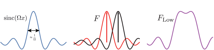
Figure 1. The Rayleigh limit. For a signal $F(x)=\sum_{j}a_{j}\delta(x-x_{j})$, its low resolution version is given by $$F_{\text{Low}}(x)={\mathcal{}F}^{-1}\left({\mathcal{}F}\left(F\right)\cdot\chi_{\left[-\Omega,\Omega\right]}\right)\asymp\sum_{j}a_{j}\operatorname{sinc}(\Omega(x-x_{j})).$$ $F_{\text{Low}}(x)$ will have peaks of width $\approx{1\over\Omega}$, and therefore it will be increasingly difficult to recover signals for which the minimal separation between the $\{x_{j}\}$’s is much smaller than ${1\over\Omega}$.

On the other hand, the case $\Delta\ll{1\over\Omega}$ (and arbitrary signed/complex amplitudes $\{a_{j}\}$) is much more difficult (see Figure 1).

The sparse SR problem has appeared already in the work by R. Prony [51], where he devised an algebraic scheme to recover the parameters $\{x_{j},a_{j}\}$ from $2d$ equispaced measurements of ${\mathcal{}F}(F)$, assuming $F$ is given by (1.1), and for arbitrary $\Delta>0$ and $|a_{j}|>0$ (see Proposition A.2 below). Since then, Prony’s method and its various extensions and generalizations have been used extensively in applied and pure mathematics and engineering ([4, 54, 48, 49, 50, 57] and references therein). While these methods provide exact recovery for $\epsilon=0$, the question of their stability (the magnitude of ${\mathcal{}K}$ in (1.4)) becomes of essential interest. For instance, if it so happens that an estimate $F^{\prime}=\sum_{j=1}^{d}a_{j}^{\prime}\delta(x-x_{j}^{\prime})$ satisfies $\min_{1\leq j\leq d}|x_{j}^{\prime}-x_{j}|\gtrapprox\Delta$, then such $F^{\prime}$ may be of little practical use in many applications (because the inner structure of the sparse signal will be determined incorrectly).

The first work which examined the stability of SR in the sub-Rayleigh regime was by D.Donoho [26]. The signal $F$ was assumed to have an infinite number of spikes $\{x_{j}\}$, constrained to a grid of step size $\Delta$, with less than one spike per unit interval on average, but whose local complexity was constrained to have no more than $d$ spikes per any interval of length $d$ (such $d$ is called the Rayleigh index). It was shown that the worst-case $\ell_{2}$ error of such $F$ (i.e. the $\ell_{2}$ norm of the coefficient sequence of the difference) from continuous measurements with a band-limit $\Omega$ and perturbation of size $\epsilon$ (in $L_{2}$ sense) scales like $\textrm{SRF}^{\alpha}\epsilon$, where $\textrm{SRF}=\frac{1}{\Omega\Delta}>1$ is the so-called super-resolution factor, and $\alpha$ satisfies $2d-1\leq\alpha\leq 2d+1$. In [24] the authors considered the case of $d$-sparse signals supported on a grid, and showed that the correct exponent should be $\alpha=2d-1$ in this case. In another recent work [39] the same scaling was shown to hold in the case of $d$-sparse signals and discrete Fourier measurements.

In the papers mentioned above, the error rate $\textrm{SRF}^{2d-1}\epsilon$ is minimax, meaning that on one hand, it is attained by a certain algorithm for all signals of interest, and on the other hand, there exist worst-case examples for which no algorithm can achieve an essentially smaller error. It turns out that these worst-case signals all have the structure of a cluster, where all the $d$ nodes $\{x_{j}\}$ appear consecutively, i.e. $x_{j}=x_{1}+(j-1)\Delta,\;j=1,\dots,d$. A natural question which arises is: if it is a-priori known that only a subset of the $d$ spikes can become clustered, can we have better reconstruction accuracy? In this paper we shall provide a positive answer to this question.

1.3. Main contributions

In this paper we consider the case where the nodes $\{x_{j}\}$ can take arbitrary real values (the so-called off-grid setting), while the amplitudes $\{a_{j}\}$ can be arbitrary complex scalars. We further assume that exactly $p$ nodes, $x_{\kappa},\ldots,x_{\kappa+p-1}$, form a small cluster of extent $h\ll\frac{1}{\Omega}$ and are approximately uniformly distributed inside the cluster, while the rest of the nodes are well-separated from the cluster and from each other (see Definition 2.5 below). The approximate uniformity is expressed by the assumption that the minimal separation between any two cluster nodes is bounded from below by $\Delta=\tau h$ for some fixed $0<\tau\leq 1$. Under these $p$-clustered assumptions, we show in Theorem 2.10, that for small enough $\epsilon$ – and, in particular, for $\epsilon\lessapprox\left(\Omega\Delta\right)^{2p-1}$, the worst case error rates of a minimax reconstruction algorithm (see Definition 2.2 below), receiving $\Phi$ satisfying (1.3) as an input, and returning an estimate $x_{j}^{\prime}=x_{j}^{\prime}(\Phi)$, $a_{j}^{\prime}=a_{j}^{\prime}(\Phi)$, satisfy

1. Non-cluster nodes:

   $$\max_{j\notin\{\kappa,\dots,\kappa+p-1\}}|x_{j}-x_{j}^{\prime}| \asymp\frac{\epsilon}{\Omega},$$

   $$\max_{j\notin\{\kappa,\dots,\kappa+p-1\}}|a_{j}-a_{j}^{\prime}| \asymp\epsilon.$$

2. Cluster nodes:

   $$\max_{j\in\{\kappa,\dots,\kappa+p-1\}}|x_{j}-x_{j}^{\prime}| \asymp\frac{\epsilon}{\Omega}\left(\Omega\Delta\right)^{-2p+2},$$

   $$\max_{j\in\{\kappa,\dots,\kappa+p-1\}}|a_{j}-a_{j}^{\prime}| \asymp\epsilon\left(\Omega\Delta\right)^{-2p+1}.$$

The constants appearing in our bounds depend on $p,d$, a-priori bounds on the magnitudes $|a_{j}|$, and additional geometric parameters, but neither on $\Delta$ nor on $\Omega$.

Our results indicate, in particular, that the non-clustered nodes $\{x_{j}\}_{j\notin\left[\kappa,\dots,\kappa+p-1\right]}$ can be recovered with much better accuracy than the cluster nodes. Let the super-resolution factor be defined, as before, by $\textrm{SRF}=\left(\Omega\Delta\right)^{-1}$, then the condition number of the cluster nodes scales like $\textrm{SRF}^{2p-1}$ in the super-resolution regime $\textrm{SRF}\gg 1$, while the condition number of the non-cluster nodes does not depend on the SRF at all.

Our approach is to reduce the continuous measurements problem to a certain “Prony-type” system of $2d$ nonlinear equations, given by equispaced measurements of $\Phi(s)$ with a carefully chosen spacing $\lambda\approx\Omega$, and analyze the sensitivity of this system to perturbations. The proofs involve techniques from quantitative singularity theory and numerical analysis. Some of the tools, in particular the “decimation-and-blowup” technique, were previously developed in [2, 6, 11, 7, 1, 13, 12, 8]. The single-cluster case $p=d$ has been first analyzed in [7], while the lower bound (in a slightly less general formulation) has been essentially shown in [1]. One of the main technical results, Lemma 5.8, has been first proven in [8].

Our numerical experiments in Section 3 show that the above bounds are attained by Matrix Pencil (MP), a well-known high-resolution algorithm [37, 36].

1.4. Related work and discussion

Our main results generalize several previously available bounds for both on-grid and off-grid SR [24, 39, 7], replacing the overall sparsity $d$ with the “local” sparsity $p$. Compared with previous works, we also have an explicit control of the perturbation $\epsilon$ for which the stability bounds hold: $\epsilon\leq C\cdot\left(\Omega\Delta\right)^{2p-1}$. So, given $F$ satisfying the clustering assumptions and $\Omega$, we can choose $\epsilon=c\left(\Omega\Delta\right)^{2p-1}$ such that $F$ can be accurately resolved, and $c$ does not depend on $\Omega,\Delta$. But this also means that given $\epsilon>0$, we can choose $\Delta_{0}$ and $\Omega_{0}$ such that $\left(\Omega_{0}\Delta_{0}\right)^{2p-1}\geq{\epsilon\over c}$, and for any $F$ satisfying the clustering assumptions with $\Delta=\Delta_{0}$ and $\Omega=\Omega_{0}$, the SR problem can be accurately solved. Therefore, fixing $\epsilon$, our results show that accurate recovery is possible for all SRF values up to $\left({1\over\epsilon}\right)^{1\over{2p-1}}$ (but possibly also for higher values of SRF). On the other hand, a similar argument using the lower bounds for the minimax error shows that with perturbation of magnitude $\epsilon$, no algorithm can resolve signals having a cluster of size $p$ and separation $\Delta_{\epsilon}\lessapprox{1\over\Omega}\epsilon^{1\over{2p-1}}$, giving an upper bound for the attainable SRF values exactly matching the lower bound above. To summarize, we obtain the best possible scaling of the attainable resolution with clustered sparsity $p$ and absolute perturbation $\epsilon$:

(1.5) $$\textrm{SRF}\asymp\sqrt[2p-1]{1\over\epsilon}.$$

This Hölder-type scaling is much more favorable compared to SR by analytic continuation under the prior of compact signal support, where the bandwidth extrapolation factor scales only as a fractional power of $\log{1\over\epsilon}$, see e.g. [9] and references therein. Also note that the sparse SR problem enjoys linear stability in $\epsilon$ (1.4), whereas analytic continuation exhibits stability of the form $Error\approx\epsilon^{\gamma}$, where $\gamma<1$ [18, 9].

Stable SR in the on-grid setting of [24, 26, 39] is closely related to the smallest singular value of a certain class of Fourier-type matrices. Using the decimation technique (see also [23, 22]), in a recent paper [8] we have derived novel estimates for this quantity under the partial clustering setting (compare with [3, 45, 15, 29, 38]), and using these results, we have shown in the same paper that the asymptotic scaling of the condition number for on-grid SR in this regime is $\textrm{SRF}^{2p-1}$, matching the off-grid setting of the present paper.

The question of providing rigorous performance guarantees for high-resolution algorithms such as MP, MUSIC, ESPRIT and others, in the super-resolution regime $\textrm{SRF}>1$, is of current interest. In two very recent works, [40, 39], the authors derive stability estimates for MUSIC and ESPRIT algorithms under similar clustering assumptions, finite sampling and white Gaussian perturbation model. Their results suggest that the corresponding noise amplification factors ${\mathcal{}K}$ for the nodes are of the order $\textrm{SRF}^{2p-2}$ with high probability. During the review of the present paper, the authors of [40] established near-optimality of ESPRIT in the bounded noise model. In particular, they showed that ESPRIT is optimal up to a factor of $1/\Omega$, i.e. $|x_{j}-\tilde{x}_{j}|\lessapprox(\Omega\Delta)^{-2p-2}\varepsilon$ with discrete Fourier measurements, however, requiring $\varepsilon\lessapprox(\Omega\Delta)^{4p-3}/\Omega$. We also mention [16, 33], where the connection between perturbation of (square) matrix pencil eigenvalues and the a-priori distribution of these eigenvalues was established via potential theory. It will be interesting to investigate the possibility to applying these methods to the analysis of MP in the clustered setting.

Turning to other techniques, the special case of a single cluster can be solved with optimal accuracy by polynomial homotopy methods, as described in [6], however in order to generalize this algorithm to configurations with non-cluster nodes, we need to know the optimal decimation parameter $\lambda$. Nonlinear least-squares and related methods (e.g., Variable Projections [32, 47]) apparently provide an optimal recovery rate, however they generally require very accurate initialization. We hope that our methods may help in analyzing these techniques as well, and plan to pursue this line of research in the future. For the case of positive point sources, stability rate $\textrm{SRF}^{2p}$ has been established for convex optimization techniques in [46], see also a related preprint [25].

1.5. Organization of the paper

In Section 2 we provide the necessary definitions and formulate the main results. In Section 3 we present several numerical experiments confirming the optimality of the Matrix Pencil algorithm. The proof of Theorem 2.6 (upper bound) is presented in Section 5. The proof of Theorem 2.8 (lower bound) is given in Section 6.

1.6. Acknowledgements

The research of GG and YY is supported in part by the Minerva Foundation. DB is supported in part by AFOSR grant FA9550-17-1-0316, NSF grant DMS-1255203, and a grant from the MIT-Skolkovo initiative.

2. Minimax bounds for clustered super-resolution

2.1. Notation and preliminaries

We shall denote by ${\mathcal{}P}_{d}$ the parameter space of signals $F$ with complex amplitudes and real, pairwise distinct and ordered nodes,

$${\mathcal{}P}_{d}=\left\{(\boldsymbol{\mathrm{a}},\boldsymbol{\mathrm{x}}):\boldsymbol{\mathrm{a}}=(a_{1},\ldots,a_{d})\in{\mathbb{C}}^{d},\;\boldsymbol{\mathrm{x}}=(x_{1},\ldots,x_{d})\in\mathbb{R}^{d},\ x_{1}<x_{2}<\ldots<x_{d}\right\},$$

and identify signals $F$ with their parameters $(\boldsymbol{\mathrm{a}},\boldsymbol{\mathrm{x}})\in{\mathcal{}P}_{d}.$ In particular, this induces a structure of a linear space on ${\mathcal{}P}_{d}$. Throughout this text we will always use the maximum norm $\|\cdot\|=\|\cdot\|_{\infty}$ on $\mathbb{C}^{d},\;\mathbb{R}^{d}$ and ${\mathcal{}P}_{d}$, where for $F=(\boldsymbol{\mathrm{a}},\boldsymbol{\mathrm{x}})\in{\mathcal{}P}_{d}$

$$\|F\|=\max\big{(}\|\boldsymbol{\mathrm{a}}\|_{\infty},\|\boldsymbol{\mathrm{x}}\|_{\infty}\big{)}.$$

We shall denote the orthogonal coordinate projections of a signal $F$ to the $j$-th node and $j$-th amplitude, respectively, by $P_{\boldsymbol{\mathrm{x}},j}:{\mathcal{}P}_{d}\to\mathbb{R}$ and $P_{\boldsymbol{\mathrm{a}},j}:{\mathcal{}P}_{d}\to\mathbb{C}$. We shall also denote the $j$-th component of a vector $\boldsymbol{\mathrm{v}}$ by $\boldsymbol{\mathrm{v}}_{j}$.

Let $L_{\infty}[-\Omega,\Omega]$ denote the space of bounded complex-valued functions defined on $[-\Omega,\Omega]$ with the norm $\|e\|=\max_{|s|\leq\Omega}\left|e(s)\right|$.

Definition 2.1.

Given $\Omega>0$ and $U\subseteq{\mathcal{}P}_{d}$, we denote by $\mathfrak{F}(\Omega,U)$ the class of all admissible reconstruction algorithms, i.e.

$$\mathfrak{F}(\Omega,U)=\biggl{\{}\mathfrak{f}:L_{\infty}\left[-\Omega,\Omega\right]\to U\biggr{\}}.$$

Definition 2.2.

Let $U\subset{\mathcal{}P}_{d}$. We consider the minimax error rate in estimating a signal $F\in U$ from $\Omega$-bandlimited data as in (1.3), with measurement error $\epsilon>0$:

$${\mathcal{}E}(\epsilon,U,\Omega)=\inf_{\mathfrak{f}\in\mathfrak{F}(\Omega,U)}\ \sup_{F\in U}\ \sup_{\|e\|\leq\epsilon}\|F-\mathfrak{f}\left({\mathcal{}F}(F)+e\right)\|.$$

Similarly the minimax errors of estimating the individual nodes, respectively, the amplitudes of $F\in U$ are defined by

$${\mathcal{}E}^{\boldsymbol{\mathrm{x}},j}(\epsilon,U,\Omega) =\inf_{\mathfrak{f}\in\mathfrak{F}(\Omega,U)}\ \sup_{F\in U}\ \sup_{\|e\|\leq\epsilon}\left|P_{\boldsymbol{\mathrm{x}},j}(F)-P_{\boldsymbol{\mathrm{x}},j}\left(\mathfrak{f}\left({\mathcal{}F}(F)+e\right)\right)\right|,$$

$${\mathcal{}E}^{\boldsymbol{\mathrm{a}},j}(\epsilon,U,\Omega) =\inf_{\mathfrak{f}\in\mathfrak{F}(\Omega,U)}\ \sup_{F\in U}\ \sup_{\|e\|\leq\epsilon}\left|P_{\boldsymbol{\mathrm{a}},j}(F)-P_{\boldsymbol{\mathrm{a}},j}\left(\mathfrak{f}({\mathcal{}F}(F)+e)\right)\right|.$$

Let a signal $F\in{\mathcal{}P}_{d}$ be fixed. We define the $\epsilon$-error set $E_{\epsilon,\Omega}(F)$ as the following pre-image.

Definition 2.3.

The error set $E_{\epsilon,\Omega}(F)\subset{\mathcal{}P}_{d}$ is the set consisting of all the signals $F^{\prime}\in{\mathcal{}P}_{d}$ with

$$\left|{\mathcal{}F}(F^{\prime})(s)-{\mathcal{}F}(F)(s)\right|\leq\epsilon, s\in[-\Omega,\Omega].$$

We will denote by $E^{\boldsymbol{\mathrm{x}},j}_{\epsilon}(F)=E^{\boldsymbol{\mathrm{x}},j}_{\epsilon,\Omega}(F)$ and $E^{\boldsymbol{\mathrm{a}},j}_{\epsilon}(F)=E^{\boldsymbol{\mathrm{a}},j}_{\epsilon,\Omega}(F)$ the projections of the error set onto the individual nodes and the amplitudes components, respectively:

(2.1) $$\begin{split}E^{\boldsymbol{\mathrm{x}},j}_{\epsilon,\Omega}(F)&=\left\{\boldsymbol{\mathrm{x}}_{j}^{\prime}\in{\mathbb{R}}:\left(\boldsymbol{\mathrm{a}}^{\prime},\boldsymbol{\mathrm{x}}^{\prime}\right)\in E_{\epsilon,\Omega}(F)\right\}\equiv P_{\boldsymbol{\mathrm{x}},j}E_{\epsilon,\Omega}(F),\\ E^{\boldsymbol{\mathrm{a}},j}_{\epsilon,\Omega}(F)&=\left\{\boldsymbol{\mathrm{a}}_{j}^{\prime}\in{\mathbb{C}}:\left(\boldsymbol{\mathrm{a}}^{\prime},\boldsymbol{\mathrm{x}}^{\prime}\right)\in E_{\epsilon,\Omega}(F)\right\}\equiv P_{\boldsymbol{\mathrm{a}},j}E_{\epsilon,\Omega}(F).\end{split}$$

For any subset $V$ of a normed vector space with norm $\|\cdot\|$, the diameter of $V$ is

$$diam(V)=\sup_{\boldsymbol{\mathrm{v}}^{\prime},\boldsymbol{\mathrm{v}}^{\prime\prime}\in V}\|\boldsymbol{\mathrm{v}}^{\prime}-\boldsymbol{\mathrm{v}}^{\prime\prime}\|.$$

The minimax errors are directly linked to the diameter of the corresponding projections of the error set by the following easy computation, which is standard in the theory of optimal recovery [43, 42, 44] (see also [26, 24, 39]).

Proposition 2.4.

For $U\subset{\mathcal{}P}_{d}$, $\Omega>0$, $1\leq j\leq d$ and $\epsilon>0$ we have

(2.2) $$\frac{1}{2}\sup_{F:\ E_{\frac{1}{2}\epsilon,\Omega}(F)\subseteq U}diam\big{(}E_{\frac{1}{2}\epsilon,\Omega}(F)\big{)} \leq{\mathcal{}E}(\epsilon,U,\Omega)\leq\sup_{F\in U}diam\big{(}E_{2\epsilon,\Omega}(F))$$

(2.3) $$\frac{1}{2}\sup_{F:\ E_{\frac{1}{2}\epsilon,\Omega}(F)\subseteq U}diam\big{(}E^{\boldsymbol{\mathrm{x}},j}_{\frac{1}{2}\epsilon,\Omega}(F)\big{)} \leq{\mathcal{}E}^{\boldsymbol{\mathrm{x}},j}(\epsilon,U,\Omega)\leq\sup_{F\in U}diam\big{(}E^{\boldsymbol{\mathrm{x}},j}_{2\epsilon,\Omega}(F))$$

(2.4) $$\frac{1}{2}\sup_{F:\ E_{\frac{1}{2}\epsilon,\Omega}(F)\subseteq U}diam\big{(}E^{\boldsymbol{\mathrm{a}},j}_{\frac{1}{2}\epsilon,\Omega}(F)\big{)} \leq{\mathcal{}E}^{\boldsymbol{\mathrm{a}},j}(\epsilon,U,\Omega)\leq\sup_{F\in U}diam\big{(}E^{\boldsymbol{\mathrm{a}},j}_{2\epsilon,\Omega}(F))$$

Proof.

We shall prove (2.2), the proof in the other cases is identical. We omit $\Omega$ from the following to reduce clutter.

Upper bound:

Let $\epsilon>0$. For any $\Phi\in L_{\infty}[-\Omega,\Omega]$, let

$${\mathcal{}B}\left(\epsilon,\Phi\right) =\left\{F\in U:\|{\mathcal{}F}(F)-\Phi\|\leq\epsilon\right\}.$$

Consider an oracle estimator $\mathfrak{f}_{\epsilon}\in\mathfrak{F}(\Omega,U)$ defined as

$$\mathfrak{f}_{\epsilon}(\Phi)=\begin{cases}\text{any element of }{\mathcal{}B}(\epsilon,\Phi)&\text{if }{\mathcal{}B}(\epsilon,\Phi)\neq\emptyset,\\ F_{0}&\text{else},\end{cases}$$

where $F_{0}$ is an arbitrary element of $U$. Now let $F\in U$, and $\Phi={\mathcal{}F}(F)+e$ where $\|e\|\leq\epsilon$. Then by definition $F\in{\mathcal{}B}(\epsilon,\Phi)$. Put $F^{\prime}=\mathfrak{f}_{\epsilon}(\Phi)$, thus $\left\|{\mathcal{}F}(F^{\prime})-\Phi\right\|\leq\epsilon$, and therefore

$$\|{\mathcal{}F}(F^{\prime})-{\mathcal{}F}(F)\|\leq\|{\mathcal{}F}(F^{\prime})-\Phi\|+\|\Phi-{\mathcal{}F}(F)\|=2\epsilon.$$

We conclude that $F^{\prime}\in E_{2\epsilon}(F)$, and consequently ${\mathcal{}E}(\epsilon,U,\Omega)\leq\|F-F^{\prime}\|\leq diam\big{(}E_{2\epsilon}(F)\big{)}$.

Lower bound:

For the lower bound, let $F\in U$ such that $E_{\frac{1}{2}\epsilon}(F)\subseteq U$. Let $\xi>0$ small enough be fixed. There exist $F^{1},\ F^{2}\in E_{\frac{1}{2}\epsilon}(F)$ with $\|F^{1}-F^{2}\|=diam\big{(}E_{\frac{1}{2}\epsilon}(F)\big{)}-\xi$. Let $\Phi={\mathcal{}F}(F)$, and let $F^{\prime}=\mathfrak{f}(\Phi)$ be the output of a certain estimator $\mathfrak{f}$ corresponding to the input $\Phi$. We have $\big{\|}\Phi-{\mathcal{}F}(F^{1})\big{\|},\ \big{\|}\Phi-{\mathcal{}F}(F^{2})\big{\|}\leq\epsilon$. Consequently, there exist perturbation functions $e_{1},e_{2}$ satisfying $\|e_{1}\|,\|e_{2}\|\leq\epsilon$, while also

$${\mathcal{}F}(F^{\prime})=\Phi ={\mathcal{}F}(F^{1})+e_{1}={\mathcal{}F}(F^{2})+e_{2}.$$

By definition of the minimax error we therefore have

$${\mathcal{}E}\left(\epsilon,U,\Omega\right) =\inf_{\mathfrak{f}}\sup_{\|e\|<\epsilon,F\in U}\|F-\mathfrak{f}({\mathcal{}F}(F)+e)\|$$

$$\geq\inf_{\mathfrak{f}}\max\left(\|F^{1}-F^{\prime}\|,\|F^{2}-F^{\prime}\|\right)$$

$$\geq\inf_{\mathfrak{f}}{1\over 2}\left\{\|F^{1}-F^{\prime}\|+\|F^{2}-F^{\prime}\|\right\}$$

$$\geq{1\over 2}\|F^{1}-F^{2}\|$$

$$={1\over 2}diam\left(E_{{1\over 2}\epsilon}(F)\right)-{\xi\over 2}.$$

The lower bound follows by letting $\xi\to 0$.

∎

2.2. Uniform estimates of minimax error for clustered configurations

The main goal of this paper is to estimate ${\mathcal{}E}\left(\epsilon,U,\Omega\right)$ (in fact its component-wise analogues ${\mathcal{}E}^{\boldsymbol{\mathrm{x}},j}\left(\epsilon,U,\Omega\right)$ and ${\mathcal{}E}^{\boldsymbol{\mathrm{a}},j}\left(\epsilon,U,\Omega\right)$) where $U\subset{\mathcal{}P}_{d}$ are certain compact subsets of ${\mathcal{}P}_{d}$ containing signals with $p\leq d$ nodes forming a small, approximately uniform, cluster. In order to have explicit bounds, we describe such sets $U$ by additional parameters $T,h,\tau,\eta,m,M$ as follows.

Definition 2.5 (Uniform cluster configuration, Figure 2).

Given $0<\tau,\eta\leq 1$ and $0<h\leq T$, a node vector $\boldsymbol{\mathrm{x}}=(x_{1},\ldots,x_{d})\in\mathbb{R}^{d}$ is said to form a $(p,h,T,\tau,\eta)$-clustered configuration, if there exists a subset of $p$ nodes $\boldsymbol{\mathrm{x}}^{c}=\{x_{\kappa},\ldots,x_{\kappa+p-1}\}\subset\boldsymbol{\mathrm{x}}$, $p\geq 2$, which satisfies the following conditions:

1. for each $x_{j},x_{k}\in\boldsymbol{\mathrm{x}}^{c},j\neq k$,

   $$\tau h\leq|x_{j}-x_{k}|\leq h;$$

2. for $x_{\ell}\in\boldsymbol{\mathrm{x}}\setminus\boldsymbol{\mathrm{x}}^{c}$ and $x_{j}\in\boldsymbol{\mathrm{x}}$, $\ell\neq j$,

   $$\eta T\leq|x_{\ell}-x_{j}|\leq T.$$

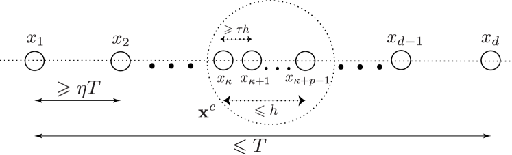
Figure 2. A sketch of a uniform $(p,h,T,\tau,\eta)$-clustered configuration $\boldsymbol{\mathrm{x}}=(x_{1},\dots,x_{d})$ as in Definition 2.5.

Our first main result provides an upper bound on $diam\left(E_{\epsilon,\Omega}(F)\right)$, and its coordinate projections, for any signal $F$ forming a clustered configuration as above.

Theorem 2.6.

(Upper bound) Let $F=(\boldsymbol{\mathrm{a}},\boldsymbol{\mathrm{x}})\in{\mathcal{}P}_{d}$, such that $\boldsymbol{\mathrm{x}}$ forms a $(p,h,T,\tau,\eta)$-clustered configuration and $0<m\leq\|\boldsymbol{\mathrm{a}}\|$. Then there exist positive constants $C_{1},\ldots,C_{5}$, depending only on $d,p,m$, such that for each $\frac{C_{4}}{\eta T}\leq\Omega\leq\frac{C_{5}}{h}$ and $\epsilon\leq C_{3}(\Omega\tau h)^{2p-1}$, it holds that:

$$diam(E^{\boldsymbol{\mathrm{x}},j}_{\epsilon,\Omega}(F)) \leq{C_{1}\over\Omega}\epsilon\times\begin{cases}(\Omega\tau h)^{-2p+2},&x_{j}\in\boldsymbol{\mathrm{x}}^{c},\\ 1,&x_{j}\in\boldsymbol{\mathrm{x}}\backslash\boldsymbol{\mathrm{x}}^{c};\end{cases}$$

$$diam(E^{\boldsymbol{\mathrm{a}},j}_{\epsilon,\Omega}(F)) \leq C_{2}\epsilon\times\begin{cases}(\Omega\tau h)^{-2p+1},&x_{j}\in\boldsymbol{\mathrm{x}}^{c},\\ 1,&x_{j}\in\boldsymbol{\mathrm{x}}\backslash\boldsymbol{\mathrm{x}}^{c}.\end{cases}$$

Remark 2.7.

Our main focus is to investigate the error rates of the SR problem as the cluster size becomes small. Fixing the parameters $p,d,m$, the range of admissible $\Omega$ in Theorem 2.6, $\frac{C_{4}}{\eta T}\leq\Omega\leq\frac{C_{5}}{h}$, is non-empty for a sufficiently small cluster size $h$. Furthermore we comment here that the constants $C_{4},C_{5}$ actually only depend on $d$.

The above estimates are order optimal, as our next main theorem shows. For simplicity and without loss of generality, in the results below we assume that the index $\kappa$ is fixed.

Theorem 2.8.

(Lower bound) Let $m\leq M,2\leq p\leq d,\tau\leq{1\over{p-1}},\eta<{1\over{d}},T>0$ be fixed. There exist positive constants $C_{1}^{\prime}\dots,C_{5}^{\prime}$, depending only on $d,p,m,M$, such that for every $\Omega,h$ satisfying $h\leq C_{4}^{\prime}T$ and $\Omega h\leq C_{5}^{\prime}$ there exists $F=(\boldsymbol{\mathrm{a}},\boldsymbol{\mathrm{x}})\in{\mathcal{}P}_{d}$, with $\boldsymbol{\mathrm{x}}$ forming a $(p,h,T,\tau,\eta)$-clustered configuration, and with $0<m\leq\|\boldsymbol{\mathrm{a}}\|\leq M<\infty$, such that for certain indices $j_{1},j_{2}\in\left\{\kappa,\dots,\kappa+p-1\right\}$ and every $\epsilon\leq C_{3}^{\prime}(\Omega\tau h)^{2p-1}$, it holds that:

$$diam(E^{\boldsymbol{\mathrm{x}},j}_{\epsilon,\Omega}(F)) \geq{C_{1}^{\prime}\over\Omega}\epsilon\times\begin{cases}(\Omega\tau h)^{-2p+2},&\text{if }j=j_{1},\\ 1,&\forall j\notin\left\{\kappa,\dots,\kappa+p-1\right\};\end{cases}$$

$$diam(E^{\boldsymbol{\mathrm{a}},j}_{\epsilon,\Omega}(F)) \geq C_{2}^{\prime}\epsilon\times\begin{cases}(\Omega\tau h)^{-2p+1},&\text{if }j=j_{2},\\ 1,&\forall j\notin\left\{\kappa,\dots,\kappa+p-1\right\}.\end{cases}$$

Remark 2.9.

The lower bounds for the quantities $diam(E^{\boldsymbol{\mathrm{x}},j}_{\epsilon,\Omega}(F))$ were shown in [1] to hold for any signal $F$ with real amplitudes, however, at the expense of the implicit dependence of the constants on the separation parameter $\tau$. While bounding $diam(E_{\epsilon,\Omega}(F))$ (and its projections) for all signals $F$ is an interesting question in its own right, in this paper we use these to bound the minimax error rate, and therefore it is sufficient to show that there exist certain signals with large enough $E_{\epsilon,\Omega}(F)$. As it turns out, it is possible to obtain a more accurate geometric description of these sets, which in turn can be used for reducing reconstruction error if additional a-priori information is available. Work in this direction was started in [2] and we intend to provide further details of these developments in a future work.

Combining Theorems 2.6 and 2.8 with Proposition 2.4, we obtain optimal rates for the minimax error ${\mathcal{}E}$ and its projections as follows.

Theorem 2.10.

Let $m<M,2\leq p\leq d,\tau<{1\over{2(p-1)}},\eta<{1\over{2d}},T>0$ be fixed. There exist constants $c_{1},c_{2},c_{3}$, depending only on $d,p,m,M$ such that for all $\frac{c_{1}}{\eta T}\leq\Omega\leq\frac{c_{2}}{h}$ and $\epsilon\leq c_{3}(\Omega\tau h)^{2p-1}$, the minimax error rates for the set

$$U: =U(p,d,h,\tau,\eta,T,m,M)$$

$$=\left\{(\boldsymbol{\mathrm{a}},\boldsymbol{\mathrm{x}})\in{\mathcal{}P}_{d}:\quad 0<m\leq\|\boldsymbol{\mathrm{a}}\|\leq M<\infty,\;\boldsymbol{\mathrm{x}}\text{ forms a }(p,h,T,\tau,\eta)\text{-clustered configuration}\right\},$$

satisfy the following.

1. For the non-cluster nodes:

   $$\forall j\notin\left\{\kappa,\dots,\kappa+p-1\right\}:\quad\begin{cases}{\mathcal{}E}^{\boldsymbol{\mathrm{x}},j}(\epsilon,U,\Omega)\asymp{\epsilon\over\Omega},\\ {\mathcal{}E}^{\boldsymbol{\mathrm{a}},j}(\epsilon,U,\Omega)\asymp\epsilon.\end{cases}$$

2. For the cluster nodes:

$$\max_{j=\kappa,\dots,\kappa+p-1}{\mathcal{}E}^{\boldsymbol{\mathrm{x}},j}(\epsilon,U,\Omega) \asymp{\epsilon\over\Omega}(\Omega\tau h)^{-2p+2},$$

$$\max_{j=\kappa,\dots,\kappa+p-1}{\mathcal{}E}^{\boldsymbol{\mathrm{a}},j}(\epsilon,U,\Omega) \asymp\epsilon(\Omega\tau h)^{-2p+1}.$$

The proportionality constants in the above statements depend only on $d,p,m,M$.

Proof.

Let $C_{3},C_{3}^{\prime},C_{4},C_{4}^{\prime},C_{5},C_{5}^{\prime}$ be the constants from Theorems 2.6 and 2.8. Put $c_{1}=C_{4}$ and $c_{2}=\min\left(C_{5},C_{5}^{\prime},C_{4}C_{4}^{\prime}\right)$. Let $\frac{c_{1}}{\eta T}\leq\Omega\leq\frac{c_{2}}{h}$, and $\epsilon\leq c_{3}(\Omega\tau h)^{2p-1}$, where $c_{3}\leq\min(C_{3},C_{3}^{\prime})$ will be determined below. It is immediately verified that $\Omega,h$ and $\epsilon$ as above satisfy the conditions of both Theorems 2.6 and 2.8.

Upper bound:

Directly follows from the upper bounds in Theorem 2.6 and Proposition 2.4.

Lower bound:

Denote $U_{\epsilon}=\left\{F\in U:E_{\frac{1}{2}\epsilon,\Omega}(F)\subseteq U\right\}$. To prove the lower bounds on ${\mathcal{}E}$, it is sufficient to show that there exists an $F\in U_{\epsilon}\neq\emptyset$ such that the conclusions of Theorem 2.8 are satisfied for this $F$.

It is not difficult to see that for any choice of the parameters as above, the set $U$ has a non-empty interior, and furthermore that one can choose $m^{\prime},M^{\prime}$ satisfying $m<m^{\prime}<M^{\prime}<M$, and also $T^{\prime}=0.99T$, $\tau^{\prime}=2\tau$ and $\eta^{\prime}=2\eta$, such that

$$U^{\prime}=U(p,d,h,\tau^{\prime},\eta^{\prime},T^{\prime},m^{\prime},M^{\prime})\subset U,\quad\partial U^{\prime}\cap\partial U=\emptyset.$$

By construction, there exist positive constants $\tilde{C_{1}},\tilde{C_{2}}$, independent of $\Omega,h$ and $\tau,\eta$, such that

(2.5) $$\begin{split}\inf_{u\in\partial U,u^{\prime}\in\partial U^{\prime}}\left|P_{\boldsymbol{\mathrm{x}},j}(u)-P_{\boldsymbol{\mathrm{x}},j}(u^{\prime})\right|&\geq\tilde{C_{1}}\times\begin{cases}\tau h,&x_{j}\in\boldsymbol{\mathrm{x}}^{c},\\ \eta T,&x_{j}\in\boldsymbol{\mathrm{x}}\setminus\boldsymbol{\mathrm{x}}^{c};\end{cases}\\ \inf_{u\in\partial U,u^{\prime}\in\partial U^{\prime}}\left|P_{\boldsymbol{\mathrm{a}},j}(u)-P_{\boldsymbol{\mathrm{a}},j}(u^{\prime})\right|&\geq\tilde{C_{2}}.\end{split}$$

Now we use the fact that $\epsilon<c_{3}(\Omega\tau h)^{2p-1}$. Applying Theorem 2.6 to an arbitrary signal $F^{\prime}\in U^{\prime}$, and using the conditions ${1\over\Omega}\leq\frac{\eta T}{c_{1}}$ and $\Omega\tau h\leq\Omega h\leq c_{2}$, we obtain that

(2.6) $$\begin{split}diam\left(E^{\boldsymbol{\mathrm{x}},j}_{{1\over 2}\epsilon}(F^{\prime})\right)&\leq\begin{cases}\frac{C_{1}c_{3}}{2}\tau h,&x_{j}\in\boldsymbol{\mathrm{x}}^{c},\\ \frac{C_{1}c_{3}}{2\Omega}(\Omega\tau h)^{2p-1}\leq\frac{C_{1}c_{3}}{2c_{1}}c_{2}^{2p-1}\eta T,&x_{j}\in\boldsymbol{\mathrm{x}}\setminus\boldsymbol{\mathrm{x}}^{c};\end{cases}\\ diam\left(E^{\boldsymbol{\mathrm{a}},j}_{{1\over 2}\epsilon}(F^{\prime})\right)&\leq\begin{cases}\frac{C_{2}c_{3}}{2},&x_{j}\in\boldsymbol{\mathrm{x}}^{c},\\ \frac{C_{2}c_{3}}{2}c_{2}^{2p-1},&x_{j}\in\boldsymbol{\mathrm{x}}\setminus\boldsymbol{\mathrm{x}}^{c}.\end{cases}\end{split}$$

Now we set $c_{3}=\min(C_{3},C_{3}^{\prime},C_{3}^{\prime\prime})$ where

$$C_{3}^{\prime\prime}=\min(1,c_{1})\times\min(1,c_{2}^{-2p+1})\times\min\biggl{(}\frac{2\tilde{C_{1}}}{C_{1}},\frac{2\tilde{C_{2}}}{C_{2}}\biggr{)}.$$

Combining (2.5) and (2.6) we obtain that $F^{\prime}\in U_{\epsilon}$. Since $F^{\prime}\in U^{\prime}$ was arbitrary, we conclude that $U^{\prime}\subseteq U_{\epsilon}$. Since clearly $U^{\prime}\neq\emptyset$, applying Proposition 2.4 and Theorem 2.8 finishes the proof.

∎

3. Numerical optimality of Matrix Pencil algorithm

The main theoretical result of this paper, Theorem 2.10, establishes the best possible scalings for the SR problem with clustered nodes. In this section we provide some numerical evidence that a certain SR algorithm, the Matrix Pencil (MP) method [37, 36], attains these performance bounds.

Our choice of MP is fairly arbitrary, as we believe that many high-resolution algorithms have similar behaviour in the regime $\textrm{SRF}\gg 1$.

Throughout this section, we replace $\Omega$ by $N$, so that the spectral data is sampled with unit spacing.

3.1. The Matrix Pencil method

Input : Model order $d$

Input : Sequence $\{\tilde{m}_{k}\},\;k=0,1,\dots,N-1$ where $N>2d$, of the form (3.1)

Input : pencil parameter $d+1\leq L\leq N-d$

Output : Estimates for the nodes $\{x_{j}\}$ and amplitudes $\{a_{j}\}$ as in (3.1)

1 Compute the matrices $A=\widetilde{H}^{\uparrow},B=\widetilde{H}_{\downarrow}$;

2 Compute the truncated Singular Value Decomposition (SVD) of $A,B$ of order $d$:

$$A=U_{1}\Sigma_{1}V_{1}^{H},\quad B=U_{2}\Sigma_{2}V_{2}^{H},$$

where $U_{1},U_{2},V_{1},V_{2}$ are $L\times d$ and $\Sigma_{1},\Sigma_{2}$ are $d\times d$ ;

3 Generate the reduced pencil

$$A^{\prime}=U_{2}^{H}U_{1}\Sigma_{1}V_{1}^{H}V_{2},\quad B^{\prime}=\Sigma_{2}$$

where $A^{\prime},B^{\prime}$ are $d\times d$;

4 Compute the generalized eigenvalues $\tilde{z}_{j}$ of the reduced pencil $(A^{\prime},B^{\prime})$ , and put $\{\tilde{x}_{j}\}=\frac{1}{2\pi}\{\angle\tilde{z}_{j}\},\;j=1,\dots,d$;

5 Compute $\tilde{a}_{j}$ by solving the linear least squares problem

$$\boldsymbol{\mathrm{\tilde{a}}}=\arg\min_{\boldsymbol{\mathrm{a}}\in\mathbb{C}^{d}}\|\boldsymbol{\mathrm{\tilde{m}}}-\tilde{V}\boldsymbol{\mathrm{a}}\|_{2},$$

where $\tilde{V}=\tilde{V}(\tilde{\boldsymbol{\mathrm{x}}})$ is the Vandermonde matrix $\tilde{V}=\left[\exp\left(2\pi\imath\tilde{x}_{j}k\right)\right]_{k=0,\dots,N-1}^{j=1,\dots,d}$;

return the estimated $\tilde{x}_{j}$ and $\tilde{a}_{j}$.

Algorithm 3.1 The Matrix Pencil algorithm

Let $F=(\boldsymbol{\mathrm{a}},\boldsymbol{\mathrm{x}})\in{\mathcal{}P}_{d}$ as in (1.1) with $x_{j}\in\left[-\frac{1}{2},\frac{1}{2}\right]$. Given the noisy Fourier measurements

(3.1) $$\begin{split}\tilde{m}_{k}&=\underbrace{{\mathcal{}F}(F)(-k)}_{=m_{k}}+n_{k}\\ &=\sum_{j=1}^{d}a_{j}\exp(2\pi\imath x_{j}k)+n_{k},\qquad k=0,1,\dots,N-1,\quad N>2d,\end{split}$$

the Matrix Pencil method estimates $\tilde{F}=\left(\tilde{\boldsymbol{\mathrm{a}}},\tilde{\boldsymbol{\mathrm{x}}}\right)$ as follows. Consider the Hankel matrix

(3.2) $$H=\begin{bmatrix}m_{0}&m_{1}&\dots&m_{N-L-1}\\ m_{1}&m_{2}&\dots&m_{N-L}\\ \vdots&\iddots&\iddots&\vdots\\ m_{L}&m_{L+1}&\dots&\dots m_{N-1}\end{bmatrix}\in\mathbb{C}^{(L+1)\times(N-L)},$$

and further let $H^{\uparrow}=H[0:L-1,:]$ and $H_{\downarrow}=H[1:L,:]$ be the $L\times(N-L)$ matrix obtained from $H$ by deleting the last (respectively, the first) row. Then it turns out that that the numbers $z_{j}=\exp(2\pi\imath x_{j})$ are the $d$ nonzero generalized eigenvalues (i.e. rank-reducing numbers) of the pencil $H_{\downarrow}-zH^{\uparrow}$. If we now construct the noisy matrices $A=\widetilde{H}^{\uparrow},B=\widetilde{H}_{\downarrow}$ from the available data $\{\tilde{m}_{k}\}_{k=0,\dots,N-1}$, we could apparently just solve the Generalized Eigenvalue Problem with $A,B$. However, if $L>d$ then the pencil $B-zA$ is close to being singular, and so an additional step of low-rank approximation is required. We summarize the MP method in Algorithm 3.1, and the interested reader is referred to the widely available literature on the subject (e.g. [37, 36, 45, 54], and references therein) for further details. Note that there exist numerous variants of MP, but, again, we believe the particular details to be immaterial for our discussion.

3.2. Experimental setup

3.2.1. Clustered node configurations

In our experiments presented below, we constructed $(p,h,T,\tau,\allowbreak\eta)$-clustered configurations with

$$\tau={1\over{p-1}},T=\pi,\eta=\frac{\pi-h}{\pi(d-p+1)}$$

as follows:

1. The cluster nodes $\boldsymbol{\mathrm{x}}^{c}=(x_{1},\dots,x_{p})$ where $x_{j}=(j-1)\cdot\Delta$ and $\Delta={h\over{p-1}}$ for $j=1,\dots,p$.

2. The non-cluster nodes were chosen to be

   $$x_{p+j}=(p-1)\Delta+j\cdot\frac{\pi-(p-1)\Delta}{d-p+1},\quad j=1,\dots,d-p.$$

3.2.2. Choice of signal and perturbation

Two different schemes were tested:

1. A generic signal with complex amplitude vector $\boldsymbol{\mathrm{a}}^{(1)}=\left(\imath^{0},\imath^{1},\imath^{2},\dots\right)\in\mathbb{C}^{d}$ and a bounded random perturbation sequence $\{n_{k}\}$, uniformly distributed in $\left[-\epsilon,\epsilon\right]$.

2. Worst-case scenario in accordance with the construction of Section 6 (and in particular of Theorem 6.2): a real amplitude vector $\boldsymbol{\mathrm{a}}^{(2)}=\left(1,-1,1,\dots,\right)\in\mathbb{R}^{d}$ and the perturbed Fourier coefficient sequence $\{\tilde{m}_{k}\}$ of the particular signal $F_{\epsilon}=(\boldsymbol{\mathrm{a}}^{\prime},\boldsymbol{\mathrm{x}}^{\prime})\in{\mathcal{}P}_{d}$ constructed according to Algorithm 3.2:

   $$\tilde{m}_{k}={\mathcal{}F}(F_{\epsilon})(-k)=\sum_{j=1}^{d}\boldsymbol{\mathrm{a}}^{\prime}_{j}\exp(2\pi\imath\boldsymbol{\mathrm{x}}^{\prime}_{j}k),\quad k=0,\dots,N-1.$$

1

Input : Signal $F=(\boldsymbol{\mathrm{a}},\boldsymbol{\mathrm{x}})\in{\mathcal{}P}_{d}$ with $\boldsymbol{\mathrm{a}}=\boldsymbol{\mathrm{a}}^{(2)}$ and cluster nodes $\boldsymbol{\mathrm{x}}^{c}=(x_{1},\dots,x_{p})$

Input : Noise level $\epsilon$

Output : The perturbed signal $F_{\epsilon}$

2 Compute the cluster center $\mu=\frac{x_{1}+x_{p}}{2}$ and put $\tilde{\boldsymbol{\mathrm{x}}}^{c}=\boldsymbol{\mathrm{x}}^{c}-\mu$ ;

3 Construct the moment vector of the centered cluster: $\boldsymbol{\mathrm{g}}=\left(\sum_{j=1}^{p}\boldsymbol{\mathrm{a}}_{j}\tilde{\boldsymbol{\mathrm{x}}}_{j}^{k}\right)_{k=0,1,\dots,2p-1}\in\mathbb{R}^{2p}$ ;

4 Construct the vector $\boldsymbol{\mathrm{g}}^{\prime}$ to be equal to $\boldsymbol{\mathrm{g}}$ except the last entry: $\boldsymbol{\mathrm{g}}^{\prime}_{k}=\boldsymbol{\mathrm{g}}_{k}$ for $k=0,1,\dots,2p-2$ and $\boldsymbol{\mathrm{g}}^{\prime}_{2p-1}=\boldsymbol{\mathrm{g}}_{2p-1}+\epsilon$ ;

5 Solve the Prony problem of order $p$ with the data $\boldsymbol{\mathrm{g}}^{\prime}$ (for $\epsilon$ small enough, a unique solution always exists – see Proposition A.3 and [13]), obtaining a signal $F^{\prime}=(\boldsymbol{\mathrm{a}}^{\prime},\boldsymbol{\mathrm{x}}^{\prime})\in{\mathcal{}P}_{p}$ ;

Move the cluster nodes back and put

$$F_{\epsilon}(x)=\sum_{j=p+1}^{d}\boldsymbol{\mathrm{a}}_{j}\delta(x-\boldsymbol{\mathrm{x}}_{j})+\sum_{j=1}^{p}\boldsymbol{\mathrm{a}}^{\prime}_{j}\delta(x-(\boldsymbol{\mathrm{x}}^{\prime}_{j}+\mu));$$

return the signal $F_{\epsilon}$.

Algorithm 3.2 The worst-case perturbation signal

1

Input : $p,d,h,N,\epsilon$

Input : Testing scheme (either S1 or S2)

2 Construct the signal $F$ and the sequence $\tilde{m}_{k}$, $k=0,\dots,N-1$ according to Subsection 3.2 ;

3 Compute the actual perturbation magnitude

$$\epsilon_{0}=\max_{k=0,\dots,N-1}|{\mathcal{}F}(F)(-k)-\tilde{m}_{k}|;$$

4Execute the MP method (Algorithm 3.1) with $L=\left\lceil{N\over 2}\right\rceil$ and obtain $F_{MP}=(\boldsymbol{\mathrm{a}}^{MP},\boldsymbol{\mathrm{x}}^{MP})$ ;

5 for each $j$ do

6       compute the error for node $j$:

$$e_{j}=\min_{\ell}|\boldsymbol{\mathrm{x}}^{MP}_{j}-\boldsymbol{\mathrm{x}}_{\ell}|;$$

7      The success for node $j$ is defined as

$$Succ_{j}=\left(e_{j}<{{\min_{\ell\neq j}|\boldsymbol{\mathrm{x}}_{\ell}-\boldsymbol{\mathrm{x}}_{j}|}\over 3}\right).$$

8      if $Succ_{j}$ == true then

9             let $\ell(j)=\arg\min_{\ell}|\boldsymbol{\mathrm{x}}^{MP}_{j}-\boldsymbol{\mathrm{x}}_{\ell}|$ ;

10             compute normalized node error amplification factor

$${\mathcal{}K}_{\boldsymbol{\mathrm{x}},j}=\frac{|\boldsymbol{\mathrm{x}}_{j}-\boldsymbol{\mathrm{x}}^{MP}_{\ell(j)}|\cdot N}{\epsilon_{0}};$$

11            compute normalized amplitude error amplification factor

$${\mathcal{}K}_{\boldsymbol{\mathrm{a}},j}=\frac{|\boldsymbol{\mathrm{a}}_{j}-\boldsymbol{\mathrm{a}}^{MP}_{\ell(j)}|}{\epsilon_{0}};$$

12      

13

return $\epsilon_{0}$, and $({\mathcal{}K}_{\boldsymbol{\mathrm{x}},j},{\mathcal{}K}_{\boldsymbol{\mathrm{a}},j},Succ_{j})$ for each node $j=1,\dots,d$.

Algorithm 3.3 A single experiment

3.3. Results

3.3.1. Error amplification factors

In the first set of experiments, we measured the actual error amplification factors ${\mathcal{}K}_{\boldsymbol{\mathrm{x}},j},{\mathcal{}K}_{\boldsymbol{\mathrm{a}},j}$ as in Algorithm 3.3 (recall also (1.4)), choosing $\epsilon,N,h$ randomly from a pre-defined numerical range. The results are presented in Figures 3 and 4 for the testing schemes S1 and S2, accordingly. The scalings of Theorem 2.10, in particular the dependence on SRF, are confirmed.

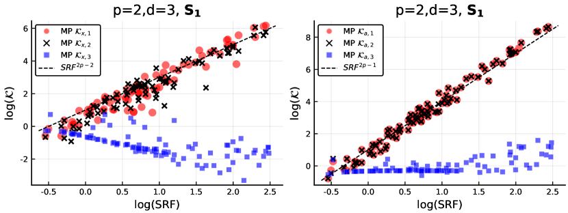
Figure 3. The error amplification factors. Algorithm 3.3 was executed 500 times with $p=2,d=3$, scheme S1 and varying $h,N,\epsilon$. For cluster nodes $j=1,2$, the node error amplification factors ${\mathcal{}K}_{\boldsymbol{\mathrm{x}},j}$ (left panel) scale like $\textrm{SRF}^{2p-2}$, while the amplitude error amplification factors ${\mathcal{}K}_{\boldsymbol{\mathrm{a}},j}$ (right panel) scale like $\textrm{SRF}^{2p-1}$. For the non-cluster node $j=3$, both error amplification factors are bounded by a constant.

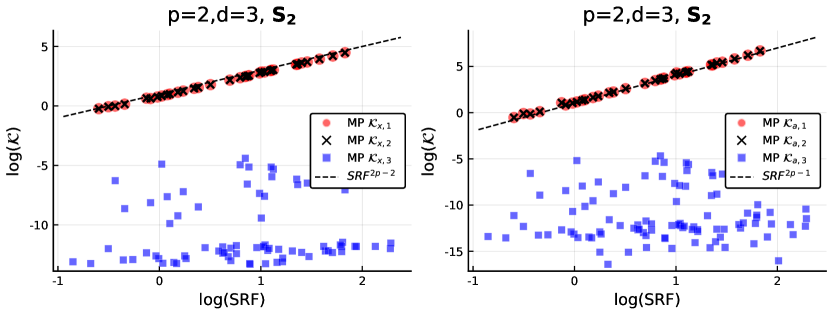
Figure 4. Same setup as in Figure 3, scheme S2. Comparing with Figure 3, the variance of the factors corresponding to the cluster nodes is much smaller than for the case of random perturbations, indicating that the construction is indeed worst-case.

3.3.2. Noise threshold for successful recovery

In the second set of experiments, we investigated the noise threshold $\epsilon\lessapprox\textrm{SRF}^{1-2p}$ for successful recovery, as predicted by the theory. We have performed $15000$ random experiments with scheme S1 (the randomness was in the choice of $h,N,\epsilon$ and the noise sequence $\{n_{k}\}$) according to Algorithm 3.3, recording the success/failure result of each such experiment. The results for $d=4$ and $p=2,3$ are presented in Figure 5, and the theoretical scaling above is confirmed for the MP method.

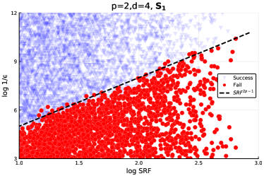
(a)

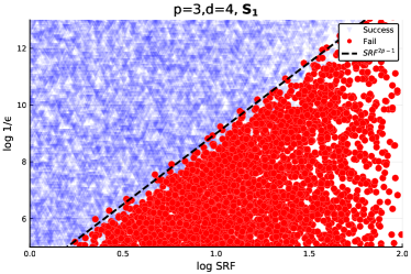
(b)

Figure 5. Phase transition for successful recovery, random bounded perturbations (scheme S1) with $d=4$ and $p=2,3$. Each experiment is represented by either a blue triangle (if the recovery was successful, i.e. $Succ_{j}==True,\;\forall j=1,\dots,d$ as returned by Algorithm 3.3) or a red circle otherwise. The relationship $\epsilon_{crit}\approx\textrm{SRF}^{1-2p}$ for the critical value of $\epsilon$ is confirmed.

Although not covered by our current theory, it is of interest to establish the recovery threshold for every node separately. In Figure 6 we can see that for a non-cluster node, the threshold is approximately constant (i.e. does not depend on the SRF) – even though Theorem 2.6 requires $\epsilon\lessapprox\textrm{SRF}^{1-2p}$.

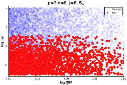
Figure 6. Phase transition for successful recovery of a non-cluster node. Comparing with Figure 5, the threshold is approximately constant $\epsilon_{crit}\approx const$. Here $p=2,d=8$, scheme S1, plotted is the successful recovery of the node at index $j=6$.

4. Normalization

In the intermediate claims, instead of considering a general signal $F=(\boldsymbol{\mathrm{a}},\boldsymbol{\mathrm{x}})\in{\mathcal{}P}_{d}$, we shall usually assume that the node vector $\boldsymbol{\mathrm{x}}=(x_{1},\dots,x_{d})$ is normalized to the interval $\left[-{1\over 2},{1\over 2}\right]$, and centered around the origin, i.e. $x_{d}=-x_{1}$. Let us briefly argue how to obtain the general result from this special case.

Let us define the scale and shift transformations on ${\mathcal{}P}_{d}$.

Definition 4.1.

For $F=\sum_{j=1}^{d}a_{j}\delta(x-x_{j})\in{\mathcal{}P}_{d}$ and $\alpha\in\mathbb{R}$, we define $SH_{\alpha}:{\mathcal{}P}_{d}\rightarrow{\mathcal{}P}_{d}$ as follows:

$$SH_{\alpha}(F)(x)=\sum_{j=1}^{d}a_{j}\delta(x-(x_{j}-\alpha)).$$

Definition 4.2.

For $F=\sum_{j=1}^{d}a_{j}\delta(x-x_{j})\in{\mathcal{}P}_{d}$ and $T>0$, we define $SC_{T}:{\mathcal{}P}_{d}\rightarrow{\mathcal{}P}_{d}$ as follows:

$$SC_{T}(F)(x)=\sum_{j=1}^{d}a_{j}\delta\left(x-\frac{x_{j}}{T}\right).$$

By the shift property of the Fourier transform, for any $\epsilon,\Omega>0$, we have that

(4.1) $$SH_{\alpha}(E_{\epsilon,\Omega}(F))=E_{\epsilon,\Omega}(SH_{\alpha}(F)).$$

By the scale property of the Fourier transform we have that for any $\epsilon>0$,

(4.2) $$SC_{T}(E_{\epsilon,\Omega}(F))=E_{\epsilon,\Omega T}(SC_{T}(F)).$$

Thus we have the following.

Proposition 4.3.

Let $F=(\boldsymbol{\mathrm{a}},\boldsymbol{\mathrm{x}})\in{\mathcal{}P}_{d}$, $\alpha\in\mathbb{R}$ and $T>0$. Then for any $\epsilon>0$ and $1\leq j\leq d$ we have

(4.3) $$diam(E^{\boldsymbol{\mathrm{x}},j}_{\epsilon,\Omega}(F))=Tdiam\left(E^{\boldsymbol{\mathrm{x}},j}_{\epsilon,\Omega T}\left(SC_{T}\left(SH_{\alpha}(F)\right)\right)\right)$$

(4.4) $$diam(E^{\boldsymbol{\mathrm{a}},j}_{\epsilon,\Omega}(F))=diam\left(E^{\boldsymbol{\mathrm{a}},j}_{\epsilon,\Omega T}\left(SC_{T}\left(SH_{\alpha}(F)\right)\right)\right)$$

5. Upper bounds

5.1. Overview of the proof

The proof of Theorem 2.6, presented in the next subsections and some of the appendices, is somewhat technical. In order to help the reader, we provide an overview of the essential ideas and steps.

The main object of the study, the error set $E_{\epsilon,\Omega}(F)\subset{\mathcal{}P}_{d}$, is the pre-image of an (infinite-dimensional) $\epsilon$-cube in the data space, under the Fourier transform mapping ${\mathcal{}F}$ (recall (1.2) and Definition 2.3). However, it is not obvious how to obtain quantitative estimates on ${\mathcal{}F}^{-1}$ directly. Thus we replace ${\mathcal{}F}$ with certain finite-dimensional sampled versions of it, denoted $FM_{\lambda}:{\mathcal{}P}_{d}\to{\mathbb{C}}^{2d}$, where the sampling parameter $\lambda$ defines the rate at which $2d$ equispaced samples of ${\mathcal{}F}(F)$ are taken. The pre-images of $\epsilon$-cubes under $FM_{\lambda}$ define the corresponding $\lambda$-error sets $E_{\epsilon,(\lambda)}\subset{\mathcal{}P}_{d}$, and in fact the original $E_{\epsilon,\Omega}(F)$ is contained in the intersection of all the $E_{\epsilon,(\lambda)}$. Thus, it is sufficient to bound the diameter of a single such $E_{\epsilon,(\lambda^{*})}$ (see remark in the next paragraph) with a carefully chosen $\lambda^{*}$ so that the result will be as small as possible. Such quantitative estimates are obtained by careful analysis of the row-wise norms of the Jacobian matrix of $FM_{\lambda^{*}}^{-1}$ and applying the so-called quantitative inverse function theorem (Theorem B.1). Using these estimates, the optimal $\lambda^{*}$ is shown to be on the order of $\Omega$, from which the upper bounds of Theorem 2.6 follow.

An additional technical complication arises from the fact that $FM_{\lambda}^{-1}$ defines a multivalued mapping, and the full pre-image $E_{\epsilon,(\lambda)}$ contains multiple copies of a certain “basic” set $A=A_{\epsilon,\lambda}$. However, when considering the intersection of all $E_{\epsilon,(\lambda)}$’s, the non-zero shifts for certain different $\lambda$’s do not intersect, and therefore eventually only the diameter of the basic set $A$ needs to be estimated.

Below is a brief description of the different intermediate results, and the organization of the remainder of Section 5.

1. In Subsection 5.2 we formally define the $\lambda$-decimated maps $FM_{\lambda}$, the corresponding error sets $E_{\epsilon,(\lambda)}$, and provide quantitative estimates on the Jacobian of $FM_{\lambda}^{-1}$ in Proposition 5.4 (proved in Appendix C). These bounds essentially depend on the “effective separation” of each node in $\boldsymbol{\mathrm{x}}$ from its neighbours, after a blowup by a factor of $\lambda$.

2. In Subsection 5.3 we show that for a signal $F=(\boldsymbol{\mathrm{a}},\boldsymbol{\mathrm{x}})$, there exist a certain range of admissible $\lambda$’s, denoted by $\Lambda(\boldsymbol{\mathrm{x}})$, for which the effective separation (see previous item) between the nodes in $\boldsymbol{\mathrm{x}}^{c}$ is of the order of $\Omega h$, while for the rest of the nodes, it is bounded from below by a constant independent of $\Omega,h$. These estimates are proved in Proposition 5.9.

3. In Subsection 5.4 we study in detail the geometry of the error sets $E_{\epsilon,(\lambda)}$ for $\lambda\in\Lambda(\boldsymbol{\mathrm{x}})$. First, we consider (in Subsection 5.4.1) the local inverses $FM_{\lambda}^{-1}$. For each $\lambda\in\Lambda(\boldsymbol{\mathrm{x}})$, we show that the local inverse exists in a neighborhood $V$ of radius $R\approx\left(\Omega h\right)^{2p-1}$ around $FM_{\lambda}(F)$, and provide estimates on the Lipschitz constants of $FM_{\lambda}^{-1}$ on $V$ and the diameter of $FM_{\lambda}^{-1}(V)$. The main bounds to that effect are proved in Proposition 5.15, using the previously established general estimates from Proposition 5.4 and the quantitative inverse function theorem (Theorem B.1).

4. Next, denoting $A=A_{R,\lambda}=FM_{\lambda}^{-1}(V)$, we show in Proposition 5.17 that the set $E_{\epsilon,(\lambda)}$ is a union of certain copies of $A$, where each such copy is obtained by shifting the nodes in $A$ by an integer multiple of $\lambda^{-1}$, and/or by permuting them.

5. In Subsection 5.5 we complete the proof. At this point we consider the entire set $\Lambda(\boldsymbol{\mathrm{x}})$. The main technical step, Proposition 5.18 (proved in Appendix F), establishes that for a certain $\lambda^{*}\in\Lambda(\boldsymbol{\mathrm{x}})$ and all possible permutations $\pi$ and shifts $\ell\in\mathbb{Z}\setminus\{0\}$, there exists a particular $\bar{\lambda}=\bar{\lambda}(\pi,\ell)\in\Lambda(\boldsymbol{\mathrm{x}})$ such that the intersection between $\pi$-permutation and $\ell$-shift of $A_{R,\lambda^{*}}$ and the entire error set $E_{R,(\bar{\lambda})}$ is empty. From this fact it immediately follows that the original error set $E_{\epsilon,\Omega}(F)$ with $\epsilon=R$ is contained in $A_{R,\lambda^{*}}$ (Proposition 5.19). The proof is finished by invoking the previously established estimates on the diameter of $A_{R,\lambda^{*}}$ and its projections.

Remark 5.1.

We expect that the tools developed throughout the proof will also be useful to calculate the minimal finite sampling rate required to achieve the minimax error rate stated in Theorem 2.6.

5.2. $\lambda$-decimation maps

For the purpose of the following analysis, we extend the space of signals ${\mathcal{}P}_{d}$ to include signals with complex nodes and denote the extended space by $\bar{{\mathcal{}P}}_{d}$,

$$\bar{{\mathcal{}P}}_{d}=\left\{(\boldsymbol{\mathrm{a}},\boldsymbol{\mathrm{x}}):\boldsymbol{\mathrm{a}}=(a_{1},\ldots,a_{d})\in{\mathbb{C}}^{d},\;\boldsymbol{\mathrm{x}}=(x_{1},\ldots,x_{d})\in{\mathbb{C}}^{d}\right\}.$$

We will be considering specific sets of exactly $2d$ samples of the Fourier transform, made at constant rate $\lambda$ as follows.

Definition 5.2.

For $\lambda>0$, we define the map $FM_{\lambda}:\bar{{\mathcal{}P}}_{d}\cong\mathbb{C}^{2d}\rightarrow\mathbb{C}^{2d}$ by

$$FM_{\lambda}((\boldsymbol{\mathrm{a}},\boldsymbol{\mathrm{x}}))=\boldsymbol{\mathrm{\mu}}=\left(\mu_{0},\dots,\mu_{2d-1}\right),\;\mu_{k}=\sum_{j=1}^{d}a_{j}e^{2\pi ix_{j}\lambda k},\ k=0,\ldots,2d-1.$$

We call such map a $\lambda$-decimation map.

For $\lambda>0$ and $\epsilon>0$, we define the corresponding error set $E_{\epsilon,(\lambda)}$ as follows.

Definition 5.3.

The error set $E_{\epsilon,(\lambda)}(F)\subset{\mathcal{}P}_{d}$ is the set consisting of all the signals $F^{\prime}\in{\mathcal{}P}_{d}$ with

$$\left\|FM_{\lambda}(F^{\prime})-FM_{\lambda}(F)\right\|\leq\epsilon.$$

Similarly we denote by $E^{\boldsymbol{\mathrm{a}},j}_{\epsilon,(\lambda)}(F),\ E^{\boldsymbol{\mathrm{x}},j}_{\epsilon,(\lambda)}(F)$ the projection of the error set $E_{\epsilon,(\lambda)}(F)$ onto the corresponding amplitudes and the nodes components (compare (2.1)).

Now consider the given spectrum ${\mathcal{}F}(F)(s),\ s\in[-\Omega,\Omega]$. Clearly for each $\lambda\leq\frac{\Omega}{2d-1}$ we have that $E_{\epsilon,\Omega}(F)\subseteq E_{\epsilon,(\lambda)}(F)$ giving

(5.1) $$E_{\epsilon,\Omega}(F)\subseteq\bigcap_{\lambda\in(0,\frac{\Omega}{2d-1}]}E_{\epsilon,(\lambda)}(F).$$

Hence, to prove the upper bounds in Theorem 2.6, we shall show that there exists a certain subset $S\subseteq\left(0,\frac{\Omega}{2d-1}\right]$ such that for each $\lambda\in S$, $diam\big{(}E_{\epsilon,(\lambda)}(F)\big{)}$ can be effectively controlled.

In the next proposition, we derive a uniform bound on the norms of the inverse Jacobian of $FM_{\lambda}$ near a signal with clustered nodes. The bounds explicitly depend on the distances between the so-called “mapped” nodes $z_{j}(\lambda)=e^{2\pi i\lambda x_{j}}$.

Proposition 5.4 (Uniform Jacobian bounds).

Let $F=(\boldsymbol{\mathrm{a}},\boldsymbol{\mathrm{x}})\in\bar{{\mathcal{}P}}_{d}$, $\boldsymbol{\mathrm{a}}=(a_{1},\dots,a_{d})$, $\boldsymbol{\mathrm{x}}=(x_{1},\ldots,x_{d})$ and for $\lambda>0$ let $z_{1}=e^{2\pi i\lambda x_{1}},\ldots,z_{d}=e^{2\pi i\lambda x_{d}}$. Suppose that for each $j=1,\ldots,d$, we have $0<\frac{m}{2}\leq|a_{j}|$ and $\frac{1}{2}\leq|z_{j}|\leq 2$ for some $m>0$.

Further assume that for $\tilde{\eta},\tilde{h}$ with $1\geq\tilde{\eta}\geq\tilde{h}$, and $\boldsymbol{\mathrm{x}}^{c}=\{x_{\kappa},\ldots,x_{\kappa+p-1}\}\subset\boldsymbol{\mathrm{x}}$, $p\geq 2$, the nodes $z_{1},\ldots,z_{d}$ satisfy:

1. For each $x_{j},x_{k}\in\boldsymbol{\mathrm{x}}^{c},j\neq k$, we have that $|z_{j}-z_{k}|\geq\tilde{h}$.

2. For each $x_{\ell}\in\boldsymbol{\mathrm{x}}\setminus\boldsymbol{\mathrm{x}}^{c}$ and $x_{j}\in\boldsymbol{\mathrm{x}}$, $\ell\neq j$, we have that $|z_{\ell}-z_{j}|\geq\tilde{\eta}$.

Then the Jacobian matrix of $FM_{\lambda}$ at $F$, denoted by $J_{\lambda}(F)$, is non-degenerate. Furthermore, write the inverse Jacobian matrix $J^{-1}_{\lambda}(F)$ in the following block form $J^{-1}_{\lambda}(F)=\begin{bmatrix}A\\ \tilde{B}\end{bmatrix}$, where $A,\tilde{B}$ are $d\times 2d$. Then, the $\ell_{1}$ norms of the rows of the blocks $A,\tilde{B}$ are bounded as follows:

(5.2) $$\sum_{k=1}^{2d}|A_{j,k}| \leq K_{1}(\tilde{\eta},d,p), x_{j}\in\boldsymbol{\mathrm{x}}\setminus\boldsymbol{\mathrm{x}}^{c},$$

(5.3) $$\sum_{k=1}^{2d}|\tilde{B}_{j,k}| \leq K_{2}(m,\tilde{\eta},d,p)\frac{1}{\lambda}, x_{j}\in\boldsymbol{\mathrm{x}}\setminus\boldsymbol{\mathrm{x}}^{c},$$

(5.4) $$\sum_{k=1}^{2d}|A_{j,k}| \leq K_{3}(\tilde{\eta},d,p)\tilde{h}^{-2p+1}, x_{j}\in\boldsymbol{\mathrm{x}}^{c},$$

(5.5) $$\sum_{k=1}^{2d}|\tilde{B}_{j,k}| \leq K_{4}(m,\tilde{\eta},d,p)\frac{1}{\lambda}\tilde{h}^{-2p+2}, x_{j}\in\boldsymbol{\mathrm{x}}^{c},$$

where $K_{1}(\cdot,\ldots,\cdot),K_{2}(\cdot,\ldots,\cdot),K_{3}(\cdot,..,,\cdot),K_{4}(\cdot,\ldots,\cdot)$ are constants depending only on the parameters inside the brackets.

The proof of Proposition 5.4 is given in Appendix C.

5.3. The existence of an admissible decimation

In this section we shall prove the existence of a certain blowup factors $\lambda$, such that the mapped nodes $\{e^{2\pi i\lambda x_{j}}\}$ (see Proposition 5.4 above) attain “good” separation properties. This result will later be used to show that for any such $\lambda$, the corresponding inverse $\lambda$-decimation map $FM_{\lambda}^{-1}$ will have the smallest possible coordinatewise Lipschitz constants with respect to $\Omega,h$ (up to constants) (see Proposition 5.4).

Definition 5.5.

For each $x\in\mathbb{R}$ and $a>0$ consider the operation $\mod{\left(-\frac{a}{2},\frac{a}{2}\right]}$ defined as

$$x\mod{\left(-\frac{a}{2},\frac{a}{2}\right]}=x-ka,$$

where $k$ is the unique integer such that $x-ka\in\left(-\frac{a}{2},\frac{a}{2}\right]$. Using this notation the principal value of the complex argument function is defined as

$$\operatorname{Arg}(re^{i\theta})=\theta\mod{(-\pi,\pi]},$$

for each $\theta\in\mathbb{R}$ and $r>0$.

Definition 5.6.

For $\alpha,\beta\in\mathbb{C}\setminus\{0\}$, we define the angular distance between $\alpha,\beta$ as

$$\angle(\alpha,\beta)=\left|\operatorname{Arg}\left(\frac{\alpha}{\beta}\right)\right|=\biggl{|}\left(\operatorname{Arg}(\alpha)-\operatorname{Arg}(\beta)\right)\ \mod{(-\pi,\pi]}\biggr{|},$$

where for $z\in\mathbb{C}\setminus\{0\}$, $\operatorname{Arg}(z)\in(-\pi,\pi]$ is the principal value of the argument of $z$.

Lemma 5.7.

For $|x|=|y|=1$, we have

(5.6) $${2\over\pi}\angle(x,y)\leq|x-y|\leq\angle(x,y).$$

Proof.

First,

$$|x-y|=\left|1-{x\over y}\right|=2\sin\left|{1\over 2}\operatorname{Arg}{x\over y}\right|=2\sin\left|{{\angle(x,y)}\over 2}\right|.$$

Then use the fact that for any $|\theta|\leq{\pi\over 2}$ we have

$${2\over\pi}|\theta|\leq\sin|\theta|\leq|\theta|\qed.$$

Let $F=(\boldsymbol{\mathrm{a}},\boldsymbol{\mathrm{x}})\in{\mathcal{}P}_{d}$ such that the node vector $\boldsymbol{\mathrm{x}}=(x_{1},\ldots,x_{d})$ forms a $(p,h,T,\tau,\eta)$-clustered configuration, with $\boldsymbol{\mathrm{x}}^{c}=\{x_{\kappa},x_{\kappa+1},\ldots,\allowbreak x_{\kappa+p-1}\}$. According to Proposition 5.4, the the norms of the rows of the inverse Jacobian $J^{-1}_{\lambda}(F)$ essentially depend on the the minimal distance between the mapped nodes $z_{j}(\lambda)=e^{2\pi i\lambda x_{j}}$. After a blowup by a factor of $\lambda\leq{1\over{2h}}$, the pairwise angular distances $\angle\left(\cdot,\cdot\right)$ (and hence the euclidean distances) between the mapped cluster-nodes $z_{\kappa},\ldots,z_{\kappa+p-1}$ are now of order $\lambda h$.

On the other hand, the non-cluster nodes are at distance larger than $\eta T\gg h$. Therefore, after the blowup by $\lambda$, the non-cluster nodes $z_{1},\ldots,z_{\kappa-1},z_{\kappa+p},\ldots,\allowbreak z_{d}$ may in principle be located anywhere on the unit circle. For example, any of these mapped non-cluster nodes might coincide with, or be very close to, a certain mapped cluster node, or yet another mapped non-cluster node.

While this situation might occur for some values of $\lambda$, we will now show that there exist certain sets of $\lambda$’s for which this does not happen. We shall require the following key estimate concerning the pairwise angular distance between any two mapped nodes.

Lemma 5.8 (A uniform blowup of two nodes).

Let $x_{j},x_{k}\in\mathbb{R},\ x_{j}\neq x_{k}$, and let $\Delta=|x_{j}-x_{k}|$. Consider the following blowups $z_{j}=z_{j}(\lambda)=e^{2\pi i\lambda x_{j}},z_{k}=z_{k}(\lambda)=e^{2\pi i\lambda x_{k}}$. Then for $0\leq\alpha\leq\pi$ and an interval $I=[a,b]\subset\mathbb{R}$, the set

(5.7) $$\Sigma^{\alpha}_{j,k}(I)=\left\{\lambda\in I:\angle\big{(}z_{j}(\lambda),z_{k}(\lambda)\big{)}\leq\alpha\right\}$$

is a union of $N$ intervals $I_{1},\ldots,I_{N}$ with $\left\lfloor|I|\Delta\right\rfloor\leq N\leq\left\lfloor|I|\Delta\right\rfloor+1$, and

$$|I_{j}|\leq\frac{\alpha}{\pi}\frac{1}{\Delta},\hskip 20.00003ptj=1,\ldots,N.$$

Proof.

For each $\lambda\in I$ we have

(5.8) $$\angle(z_{j}(\lambda),z_{k}(\lambda))=\left|\operatorname{Arg}\left(\frac{z_{j}(\lambda)}{z_{k}(\lambda)}\right)\right|=\left|\operatorname{Arg}(e^{2\pi i\lambda\Delta})\right|.$$

By equation (5.8) we have

$$\left\{\lambda\in I:\angle\big{(}z_{j}(\lambda),z_{k}(\lambda)\big{)}\leq\alpha\right\}=$$

$$\left\{\lambda\in I:\left|\operatorname{Arg}(e^{2\pi i\lambda\Delta})\right|\leq\alpha\right\}=$$

$$\left\{\lambda\in I:\left|2\pi\lambda\Delta\mod{\left(-\pi,\pi\right]}\right|\leq\alpha\right\}=$$

$$\left\{\lambda\in I:-\alpha\leq\left(2\pi\lambda\Delta\mod{\left(-\pi,\pi\right]}\right)\leq\alpha\right\}=$$

$$\left\{\lambda\in I:-\frac{\alpha}{2\pi}\frac{1}{\Delta}\leq\left(\lambda\mod{\left(-\frac{1}{2\Delta},\frac{1}{2\Delta}\right]}\right)\leq\frac{\alpha}{2\pi}\frac{1}{\Delta}\right\}.$$

The last set above can be written as $I\cap S^{\alpha}$ where

(5.9) $$S^{\alpha}=\left\{\lambda\in\mathbb{R}:-\frac{\alpha}{2\pi}\frac{1}{\Delta}\leq\left(\lambda\mod{\left(-\frac{1}{2\Delta},\frac{1}{2\Delta}\right]}\right)\leq\frac{\alpha}{2\pi}\frac{1}{\Delta}\right\}.$$

Define the interval $I^{\alpha}=\left[-\frac{\alpha}{2\pi}\frac{1}{\Delta},\frac{\alpha}{2\pi}\frac{1}{\Delta}\right]$. Then the set $S^{\alpha}$ is a union of intervals of length $\frac{\alpha}{\pi}\frac{1}{\Delta}$ as follows

$$S^{\alpha}=\bigcup_{\ell\in\mathbb{Z}}\left(I^{\alpha}+\frac{\ell}{\Delta}\right)=\bigcup_{\ell\in\mathbb{Z}}\left\{\lambda+\frac{\ell}{\Delta}:\lambda\in I^{\alpha}\right\}.$$

The intersection of $S^{\alpha}$ with any interval $I$ is then a union of $\left\lfloor|I|\Delta\right\rfloor\leq N\leq\left\lfloor|I|\Delta\right\rfloor+1$ intervals of length smaller or equal to $\frac{\alpha}{\pi}\frac{1}{\Delta}$. This concludes the proof of Lemma 5.8. ∎

Now we state and prove the main result of this subsection.

Proposition 5.9.

Let $F=(\boldsymbol{\mathrm{a}},\boldsymbol{\mathrm{x}})\in{\mathcal{}P}_{d},\ \boldsymbol{\mathrm{x}}=(x_{1},\ldots,x_{d})\subset[-\frac{1}{2},\frac{1}{2}]$, such that $\boldsymbol{\mathrm{x}}$ forms a $(p,h,1,\tau,\eta)$-clustered configuration with $\boldsymbol{\mathrm{x}}^{c}=\{x_{\kappa},x_{\kappa+1},\ldots,\allowbreak x_{\kappa+p-1}\}$.

Let $\Omega\leq\frac{2d-1}{2}\cdot{1\over h}$. For each $\lambda>0$ let $z_{1}(\lambda)=e^{2\pi i\lambda x_{1}},\ldots,z_{d}(\lambda)=e^{2\pi i\lambda x_{d}}$.

Then each interval $I\subset\left[\frac{1}{2}\frac{\Omega}{2d-1},\frac{\Omega}{2d-1}\right]$ of length $|I|=\frac{1}{\eta}$ contains a sub-interval $I^{\prime}\subset I$ of length $|I^{\prime}|\geq(2d^{2}\eta)^{-1}$ such that for each $\lambda\in I^{\prime}$:

1. For all $x_{\ell}\in\boldsymbol{\mathrm{x}}\setminus\boldsymbol{\mathrm{x}}^{c}$ and $x_{j}\in\boldsymbol{\mathrm{x}}$, $x_{j}\neq x_{\ell}$,

   (5.10) $$\angle(z_{\ell}(\lambda),z_{j}(\lambda)) \geq\frac{1}{d^{2}}.$$

2. For all $x_{j},x_{k}\in\boldsymbol{\mathrm{x}}^{c},x_{k}\neq x_{j},$

   (5.11) $$\angle(z_{j}(\lambda),z_{k}(\lambda)) \geq 2\pi\lambda\tau h\geq\frac{\pi\tau}{2d-1}\Omega h.$$

Proof.

Let us first prove that assertion (5.11) holds for any $\frac{1}{2}\frac{\Omega}{2d-1}\leq\lambda\leq\frac{\Omega}{2d-1}$.

Let $x_{j},x_{k}$, $j>k$, be two cluster nodes. The angular distance between the mapped cluster nodes $z_{j}=z_{j}(\lambda)=e^{2\pi i\lambda x_{j}},\ z_{k}=z_{k}(\lambda)=e^{2\pi i\lambda x_{k}}$, is

$$\angle(z_{j},z_{k})=\left|\operatorname{Arg}(e^{2\pi i\lambda(x_{j}-x_{k})})\right|.$$

By assumption $\Omega h\leq\frac{2d-1}{2}$, then $\lambda\leq\frac{1}{2h}$ and then $0\leq 2\pi\lambda(x_{j}-x_{k})\leq 2\pi\lambda h\leq\pi$. With this we have

$$\angle(z_{j},z_{k})=2\pi\lambda(x_{j}-x_{k})\geq 2\pi\lambda\tau h.$$

By assumption $\lambda\geq\frac{1}{2}\frac{\Omega}{2d-1}$. Then, $\angle(z_{j},z_{k})\geq\frac{\pi\tau}{2d-1}\Omega h$. This concludes the proof of assertion (5.11).

Using Lemma 5.8 we now prove that assertion (5.10) holds for any interval $I=[a,b]\subset\mathbb{R}$ of length $|I|=\frac{1}{\eta}$. Let $I$ be such an interval. For each $0<\alpha\leq\pi$ consider the set

$$\Sigma^{\alpha}(I)=\left\{\lambda\in I:\exists x_{\ell}\in\boldsymbol{\mathrm{x}}\setminus\boldsymbol{\mathrm{x}}^{c}\text{ s.t. }\min_{1\leq j\leq d,j\neq\ell}\angle(z_{\ell}(\lambda),z_{j}(\lambda))\leq\alpha\right\}.$$

We then have

$$\Sigma^{\alpha}(I)=\bigcup_{x_{\ell}\in\boldsymbol{\mathrm{x}}\setminus\boldsymbol{\mathrm{x}}^{c}}\bigcup_{x_{j}\neq x_{\ell}}\Sigma^{\alpha}_{\ell,j}(I),$$

where $\Sigma^{\alpha}_{\ell,j}$ are given by (5.7). By Lemma 5.8 each $\Sigma^{\alpha}_{\ell,j}(I)$ above is a union of at most $\left\lfloor|I|\eta\right\rfloor+1=2$ intervals, the length of each interval is at most $\frac{\alpha}{\pi}\frac{1}{\eta}$. Therefore $\Sigma^{\alpha}(I)$ is a union of at most $K=\binom{d}{2}2=d(d-1)$ intervals. Moreover, let $\nu$ denote the Lebesgue measure on $\mathbb{R}$, then

(5.12) $$\nu(\Sigma^{\alpha}(I))\leq K\frac{\alpha}{\pi}\frac{1}{\eta}\leq d(d-1)\frac{\alpha}{\pi}\frac{1}{\eta}\leq d^{2}\alpha\frac{1}{2\eta}.$$

Put $\alpha^{\prime}=\frac{1}{d^{2}}$ then by (5.12)

(5.13) $$\nu(\Sigma^{\alpha^{\prime}}(I))\leq\frac{1}{2\eta}.$$

Now consider the complement set of $\Sigma^{\alpha^{\prime}}(I)$ with respect to $I$,

$$(\Sigma^{\alpha^{\prime}}(I))^{c}=\left\{\lambda\in I:\forall x_{\ell}\in\boldsymbol{\mathrm{x}}\setminus\boldsymbol{\mathrm{x}}^{c},\min_{1\leq j\leq d,j\neq\ell}\angle(z_{\ell}(\lambda),z_{j}(\lambda))>\frac{1}{d^{2}}\right\}.$$

By (5.13)

(5.14) $$\nu\big{(}(\Sigma^{\alpha^{\prime}}(I))^{c}\big{)}\geq|I|-\frac{1}{2\eta}=\frac{1}{\eta}-\frac{1}{2\eta}=\frac{1}{2\eta}.$$

In addition, since $\Sigma^{\alpha^{\prime}}(I)$ is a union of at most $K=d(d-1)$ intervals, then $\big{(}\Sigma^{\alpha^{\prime}}(I)\big{)}^{c}$ is a union of at most

(5.15) $$L=K+1=d(d-1)+1\leq d^{2}$$

intervals. Using (5.14) and (5.15), the average size of these intervals is bounded as follows:

$$\frac{\nu\big{(}(\Sigma^{\alpha^{\prime}}(I))^{c}\big{)}}{L}\geq\frac{1}{d^{2}}\frac{1}{2\eta}.$$

We therefore conclude that $\big{(}\Sigma^{\alpha^{\prime}}(I)\big{)}^{c}$ contains an interval of length greater or equal to $\frac{1}{d^{2}}\frac{1}{2\eta}$. This proves assertion (5.10) of Proposition 5.9. ∎

5.4. Error sets of admissible decimation maps

Throughout this section we fix a signal $F=(\boldsymbol{\mathrm{a}},\boldsymbol{\mathrm{x}})\in{\mathcal{}P}_{d},\ \boldsymbol{\mathrm{a}}=(a_{1},\ldots,a_{d}),\ \boldsymbol{\mathrm{x}}=(x_{1},\ldots,x_{d})\subset\left[-\frac{1}{2},\frac{1}{2}\right]$, such that $\boldsymbol{\mathrm{x}}$ forms a $(p,h,1,\tau,\eta)$-clustered configuration, with $\boldsymbol{\mathrm{x}}^{c}=\{x_{\kappa},x_{\kappa+1},\allowbreak\ldots,x_{\kappa+p-1}\}$ and $\|\boldsymbol{\mathrm{a}}\|\geq m>0$. We also fix $\Omega>0$ such that $\Omega h\leq\frac{1}{20d}$.

Proposition 5.9 demonstrated the existence of certain $\lambda$-decimation maps which achieve good separation of the non-cluster nodes. We define the set $\Lambda(\boldsymbol{\mathrm{x}})$ to consist of all such admissible $\lambda$’s, as follows.

Definition 5.10 (Admissible blowup factors).

For each $F=(\boldsymbol{\mathrm{a}},\boldsymbol{\mathrm{x}})\in{\mathcal{}P}_{d},\ \boldsymbol{\mathrm{x}}=(x_{1},\allowbreak\ldots,x_{d})$, such that $\boldsymbol{\mathrm{x}}$ forms a $(p,h,1,\tau,\eta)$-clustered configuration and $z_{j}=z_{j}(\lambda)=e^{2\pi i\lambda x_{j}},\ j=1,\ldots,d$ and $\Omega>0$, we define the set of admissible blowup factors $\Lambda(\boldsymbol{\mathrm{x}})=\Lambda_{\Omega,d}(\boldsymbol{\mathrm{x}})$ as the set of all $\lambda\in\left[\frac{1}{2}\frac{\Omega}{2d-1},\frac{\Omega}{2d-1}\right]$ satisfying:

1. For all $\ell\neq j$ such that $x_{\ell}\in\boldsymbol{\mathrm{x}}\setminus\boldsymbol{\mathrm{x}}^{c}$ and $x_{j}\in\boldsymbol{\mathrm{x}}$,

   (5.16) $$\angle(z_{\ell}(\lambda),z_{j}(\lambda)) \geq\frac{1}{d^{2}}.$$

2. For all $j\neq k$ such that $x_{j},x_{k}\in\boldsymbol{\mathrm{x}}^{c}$

   (5.17) $$\angle(z_{j}(\lambda),z_{k}(\lambda)) \geq 2\pi\lambda\tau h\geq\frac{\pi}{2d-1}\Omega\tau h.$$

5.4.1. The local geometry of admissible decimation maps

The next result gives an explicit description of a neighborhood around $F$ where the map $FM_{\lambda}$ is injective (and, therefore, we can speak about a local inverse).

Definition 5.11.

For each $\alpha,\beta>0$ we denote by $H_{\alpha,\beta}(F)$ the closed polydisc

$$H_{\alpha,\beta}(F)=\left\{(\boldsymbol{\mathrm{a}}^{\prime},\boldsymbol{\mathrm{x}}^{\prime})\in\bar{{\mathcal{}P}}_{d}\ :\|\boldsymbol{\mathrm{a}}^{\prime}-\boldsymbol{\mathrm{a}}\|\leq\alpha,\ \|\boldsymbol{\mathrm{x}}^{\prime}-\boldsymbol{\mathrm{x}}\|\leq\beta\right\},$$

and by $H^{\mathrm{o}}_{\alpha,\beta}(F)$ the interior of $H_{\alpha,\beta}(F)$.

The following is proved in Appendix D.

Proposition 5.12 (One-to-one).

For each $\lambda\in\Lambda(\boldsymbol{\mathrm{x}})$ the map $FM_{\lambda}$ is injective in the open polydisc $U=H^{\mathrm{o}}_{m,\frac{\tau h}{2\pi}}(F)\subset\bar{{\mathcal{}P}}_{d}$.

Next we can estimate the Lipschitz constants of the inverse map $FM_{\lambda}^{-1}$, using the previously established general bounds in Proposition 5.4.

Proposition 5.13.

Let $H=H_{\frac{m}{2},\frac{\tau h}{4\pi}}(F)\subset U=H^{\mathrm{o}}_{m,\frac{\tau h}{2\pi}}(F)$. Then, for each $F^{\prime}\in H$:

1. The Jacobian matrix of $FM_{\lambda}$ at $F^{\prime}$, denoted by $J_{\lambda}(F^{\prime})$, is non-degenerate.

2. Put $J^{-1}_{\lambda}(F^{\prime})=\begin{bmatrix}A\\ \tilde{B}\end{bmatrix}$, where $A,\tilde{B}$ are $d\times 2d$. Then, the $\ell_{1}$ norms of the rows of the blocks $A,\tilde{B}$ are bounded as follows:

   (5.18) $$\sum_{k=1}^{2d}|A_{j,k}| \leq\tilde{C}, x_{j}\in\boldsymbol{\mathrm{x}}\setminus\boldsymbol{\mathrm{x}}^{c},$$

   (5.19) $$\sum_{k=1}^{2d}|\tilde{B}_{j,k}| \leq\tilde{C}\frac{1}{\Omega}, x_{j}\in\boldsymbol{\mathrm{x}}\setminus\boldsymbol{\mathrm{x}}^{c},$$

   (5.20) $$\sum_{k=1}^{2d}|A_{j,k}| \leq\tilde{C}(\Omega\tau h)^{-2p+1}, x_{j}\in\boldsymbol{\mathrm{x}}^{c},$$

   (5.21) $$\sum_{k=1}^{2d}|\tilde{B}_{j,k}| \leq\tilde{C}\frac{1}{\Omega}(\Omega\tau h)^{-2p+2}, x_{j}\in\boldsymbol{\mathrm{x}}^{c},$$

   where $\tilde{C}=\tilde{C}(m,d,p)$ is a constant depending only on $d,m,p$.

Proof.

Let $F^{\prime}=(\boldsymbol{\mathrm{a}}^{\prime},\boldsymbol{\mathrm{x}}^{\prime})\in H,\ \boldsymbol{\mathrm{a}}^{\prime}=(a^{\prime}_{1},\ldots,a^{\prime}_{d}),\ \boldsymbol{\mathrm{x}}^{\prime}=(x_{1}^{\prime},\ldots,x_{d}^{\prime})$. Let $z^{\prime}_{j}=z^{\prime}_{j}(\lambda)=e^{2\pi i\lambda x^{\prime}_{j}}$ and let $z_{j}=z_{j}(\lambda)=e^{2\pi i\lambda x_{j}},\ j=1,\ldots,d$.

By the integral mean value theorem, for each $j=1,\ldots,d$,

$$|z^{\prime}_{j}-z_{j}|=\left|e^{2\pi i\lambda x^{\prime}_{j}}-e^{2\pi i\lambda x_{j}}\right|\leq\lambda\tau h.$$

Let $\ell\neq j$ such that $x_{\ell}\in\boldsymbol{\mathrm{x}}\setminus\boldsymbol{\mathrm{x}}^{c}$ and $x_{j}\in\boldsymbol{\mathrm{x}}$. Since $\lambda\in\Lambda(x)$,

$$\angle(z_{\ell},z_{j}) \geq\frac{1}{d^{2}}.$$

Then by (5.6)

$$|z_{\ell}-z_{j}|\geq\frac{2}{\pi d^{2}}.$$

We get that

$$|z_{\ell}^{\prime}-z_{j}^{\prime}|\geq|z_{\ell}-z_{j}|-|z^{\prime}_{\ell}-z_{\ell}|-|z_{j}^{\prime}-z_{j}|\geq|z_{\ell}-z_{j}|-2\lambda\tau h\geq\frac{2}{\pi d^{2}}-2\lambda\tau h.$$

With $\Omega h\leq\frac{1}{20d}$ and $\lambda\leq\frac{\Omega}{2d-1}$ by assumption, we have that $2\lambda\tau h\leq\frac{1}{3\pi d^{2}}$ then

$$|z_{\ell}^{\prime}-z_{j}^{\prime}|\geq\frac{2}{\pi d^{2}}-2\lambda\tau h\geq\frac{2}{\pi d^{2}}-\frac{1}{3\pi d^{2}}\geq\frac{1}{2d^{2}}.$$

We conclude that for each $\ell\neq j$ such that $x_{\ell}\in\boldsymbol{\mathrm{x}}\setminus\boldsymbol{\mathrm{x}}^{c}$ and $x_{j}\in\boldsymbol{\mathrm{x}}$

(5.22) $$|z_{\ell}^{\prime}-z_{j}^{\prime}|\geq\frac{1}{2d^{2}}.$$

Let $j\neq k$ such that $x_{j},x_{k}\in\boldsymbol{\mathrm{x}}^{c}$. $\lambda\in\Lambda(\boldsymbol{\mathrm{x}})$ then

$$\angle(z_{j},z_{k}) \geq 2\pi\lambda\tau h.$$

Then by (5.6)

$$|z_{j}-z_{k}|\geq 4\lambda\tau h.$$

With a similar argument as above, we get that

$$|z_{j}^{\prime}-z_{k}^{\prime}|\geq|z_{j}-z_{k}|-2\lambda\tau h\geq 2\lambda\tau h.$$

Using $\lambda\in\Lambda(\boldsymbol{\mathrm{x}})\Rightarrow\lambda\geq\frac{\Omega}{2(2d-1)}$, we conclude that for each $j\neq k$ such that $x_{j},x_{k}\in\boldsymbol{\mathrm{x}}^{c}$

(5.23) $$|z_{j}^{\prime}-z_{k}^{\prime}|\geq 2\lambda\tau h\geq\frac{1}{2d-1}\Omega\tau h.$$

Now using (5.22) and (5.23) we invoke Proposition 5.4 with $\tilde{h}=\frac{1}{2d-1}\Omega\tau h$ and $\tilde{\eta}=\frac{1}{2d^{2}}$ and as a result prove Proposition 5.13 with

$$\tilde{C}=\left(2d-1\right)^{2p-1}\max\bigg{[}K_{1}\left(\frac{1}{2d^{2}},d,p\right),K_{2}\left(m,\frac{1}{2d^{2}},d,p\right),$$

$$K_{3}\left(\frac{1}{2d^{2}},d,p\right),K_{4}\left(m,\frac{1}{2d^{2}},d,p\right)\bigg{]}.$$

∎

Definition 5.14.

For $\boldsymbol{\mathrm{v}}\in\mathbb{C}^{d}$ and $r>0$, we denote by $Q_{r}(\boldsymbol{\mathrm{v}})$ the closed cube of radius $r$ centered at $\boldsymbol{\mathrm{v}}$:

$$Q_{r}(\boldsymbol{\mathrm{v}})=Q_{r,d}(\boldsymbol{\mathrm{v}})=\left\{\boldsymbol{\mathrm{u}}\in\mathbb{C}^{d}:\|\boldsymbol{\mathrm{u}}-\boldsymbol{\mathrm{v}}\|\leq r\right\}.$$

Proposition 5.15.

Let $U=H^{\mathrm{o}}_{m,\frac{\tau h}{2\pi}}(F)$ and $H=H_{\frac{m}{2},\frac{\tau h}{4\pi}}(F)\subset U$. Let $\lambda\in\Lambda(\boldsymbol{\mathrm{x}})$ and let $\boldsymbol{\mathrm{\mu}}_{\lambda}=FM_{\lambda}(F)$, then there exists a constant $\tilde{C}_{3}=\tilde{C}_{3}(m,d,\allowbreak p)$ such that for $R=\tilde{C}_{3}(\Omega\tau h)^{2p-1}$,

$$FM_{\lambda}(H)\supseteq Q_{R}(\boldsymbol{\mathrm{\mu}}_{\lambda}).$$

Furthermore for $V_{\lambda}=FM_{\lambda}(U)$ let

$$FM_{\lambda}^{-1}:V_{\lambda}\rightarrow U$$

be the local inverse of $FM_{\lambda}$, i.e. for all $F^{\prime}\in U$ we have $FM_{\lambda}^{-1}(FM_{\lambda}(F^{\prime}))=F^{\prime}$. For each $1\leq j\leq d$, let $P_{\boldsymbol{\mathrm{a}},j},P_{\boldsymbol{\mathrm{x}},j}:\bar{{\mathcal{}P}}_{d}\rightarrow\mathbb{C}$ be the projections onto the $j^{th}$ amplitude and the $j^{th}$ node coordinates respectively. Then $FM_{\lambda}^{-1}$ is Lipschitz on $Q_{R}(\boldsymbol{\mathrm{\mu}}_{\lambda})$ with the following bounds:

$$\left|P_{\boldsymbol{\mathrm{x}},j}FM^{-1}_{\lambda}(\boldsymbol{\mathrm{\mu}}^{\prime})-P_{\boldsymbol{\mathrm{x}},j}FM^{-1}_{\lambda}(\boldsymbol{\mathrm{\mu}}^{\prime\prime})\right| \leq\tilde{C}_{1}\frac{1}{\Omega}\|\boldsymbol{\mathrm{\mu}}^{\prime\prime}-\boldsymbol{\mathrm{\mu}}^{\prime}\|\times\begin{cases}1&x_{j}\in\boldsymbol{\mathrm{x}}\setminus\boldsymbol{\mathrm{x}}^{c}\\ (\Omega\tau h)^{-2p+2}&x_{j}\in\boldsymbol{\mathrm{x}}^{c}\end{cases},$$

$$\left|P_{\boldsymbol{\mathrm{a}},j}FM^{-1}_{\lambda}(\boldsymbol{\mathrm{\mu}}^{\prime})-P_{\boldsymbol{\mathrm{a}},j}FM^{-1}_{\lambda}(\boldsymbol{\mathrm{\mu}}^{\prime\prime})\right| \leq\tilde{C}_{2}\|\boldsymbol{\mathrm{\mu}}^{\prime\prime}-\boldsymbol{\mathrm{\mu}}^{\prime}\|\times\begin{cases}1&x_{j}\in\boldsymbol{\mathrm{x}}\setminus\boldsymbol{\mathrm{x}}^{c}\\ (\Omega\tau h)^{-2p+1}&x_{j}\in\boldsymbol{\mathrm{x}}^{c}\end{cases},$$

for each $\boldsymbol{\mathrm{\mu}}^{\prime\prime},\boldsymbol{\mathrm{\mu}}^{\prime}\in Q_{R}(\boldsymbol{\mathrm{\mu}}_{\lambda})$, where $\tilde{C}_{1}=\tilde{C}_{1}(m,d,p),\ \tilde{C}_{2}=\tilde{C}_{2}(m,d,p)$ are constants depending only on $d,m,p$ and $\tilde{C}_{1}\tilde{C}_{3}\leq 1$.

Proof.

By Proposition 5.12 $FM_{\lambda}$ is injective in the open neighborhood $U$ of the polydisc $H=H_{\frac{m}{2},\frac{\tau h}{4\pi}}(F)$. In addition, for each $F^{\prime}\in H$ the inverse Jacobian norm bounds derived in Proposition 5.13 apply. Finally one can verify (using a similar argument as in the proof of Proposition 5.13 ) that $J_{\lambda}(F^{\prime})$ is non-degenerate for each $F^{\prime}\in U$. We can therefore invoke Theorem B.1 with $U,H$ and $f=FM_{\lambda}$ and the bounds (5.18), (5.19), (5.20), (5.21), and conclude that Proposition 5.15 holds with $\tilde{C}_{1}=\tilde{C}_{2}=\tilde{C}$ and $\tilde{C}_{3}=\min\left(\frac{m}{2\tilde{C}},\frac{1}{4\pi\tilde{C}}\right)$. ∎

5.4.2. The global geometry of admissible decimation maps

In this subsection we give a global description of the geometry of the error set $E_{\epsilon,(\lambda)}(F)$ for any $\lambda\in\Lambda(\boldsymbol{\mathrm{x}})$ and for $\epsilon\leq R$ where $R=\tilde{C}_{3}(\Omega\tau h)^{2p-1}$, and $\tilde{C}_{3}$ is as specified in Proposition 5.15.

For each $\lambda\in\Lambda(\boldsymbol{\mathrm{x}})$ let $\boldsymbol{\mathrm{\mu}}_{\lambda}=FM_{\lambda}(F)$, and put

(5.24) $$A_{\epsilon,\lambda}(F)=FM_{\lambda}^{-1}\left(Q_{\epsilon}(\boldsymbol{\mathrm{\mu}}_{\lambda})\right)\bigcap{\mathcal{}P}_{d},$$

where $FM_{\lambda}^{-1}:V_{\lambda}\rightarrow U$ is the local inverse of $FM_{\lambda}$ on $U$.

Observe that $A_{\epsilon,\lambda}(F)\subset E_{\epsilon,(\lambda)}(F)$. The analysis of this subsection will reveal that globally $E_{\epsilon,(\lambda)}(F)$ is made from certain periodic repetitions of the set $A_{\epsilon,\lambda}(F)$ and its permutations.

Consider the following example.

Example 5.16.

Let $F(x)=\delta(x-\frac{1}{10})+\delta(x-\frac{2}{10})$ and let $\lambda=\frac{10}{3}$. Applying $FM_{\lambda}$ on $F$ we get that

$$FM_{\lambda}(F)=(2,e^{\frac{2\pi}{3}i}+e^{-\frac{2\pi}{3}i},e^{-\frac{2\pi}{3}i}+e^{\frac{2\pi}{3}i},2)=(2,-1,-1,2).$$

If we set $F=(\boldsymbol{\mathrm{a}},\boldsymbol{\mathrm{x}})$ with $\boldsymbol{\mathrm{a}}=(a_{1},a_{2})=(1,1)$ and $\boldsymbol{\mathrm{x}}=(x_{1},x_{2})=(\frac{1}{10},\frac{2}{10})$ then clearly the signal $F^{\prime}=(\boldsymbol{\mathrm{a}},\boldsymbol{\mathrm{x}}^{\prime})$, $\boldsymbol{\mathrm{x}}^{\prime}=(x_{2},x_{1})=(\frac{2}{10},\frac{1}{10})$, that is attained by permuting the nodes of the signal $F$, satisfies that $FM_{\lambda}(F)=FM_{\lambda}(F^{\prime})$. Observe that $F^{\prime}\notin{\mathcal{}P}_{2}$ since its nodes are not in ascending order (a condition that was posed on ${\mathcal{}P}_{d}$ to avoid redundant solutions). However, the signal $F^{\prime\prime}=(a,\boldsymbol{\mathrm{x}}^{\prime\prime})$ with $\boldsymbol{\mathrm{x}}^{\prime\prime}=\boldsymbol{\mathrm{x}}^{\prime}-\frac{1}{\lambda}(1,0)=\boldsymbol{\mathrm{x}}^{\prime}-\frac{3}{10}(1,0)=(-\frac{1}{10},\frac{1}{10})$, is in ${\mathcal{}P}_{2}$ and it holds that $FM_{\lambda}(F)=FM_{\lambda}(F^{\prime\prime})$.

One can verify that the set of signals $G\in{\mathcal{}P}_{2}$, which satisfies $FM_{\lambda}(G)=FM_{\lambda}(F)$ is given by

$$\left\{G=(\boldsymbol{\mathrm{a}},\boldsymbol{\mathrm{y}})\in{\mathcal{}P}_{2}:\boldsymbol{\mathrm{y}}=\boldsymbol{\mathrm{x}}+\frac{1}{\lambda}(n_{1},n_{2}),\ \ n_{1},n_{2}\in\mathbb{Z}\right\} \bigcup$$

$$\left\{G=(\boldsymbol{\mathrm{a}},\boldsymbol{\mathrm{y}})\in{\mathcal{}P}_{2}:\boldsymbol{\mathrm{y}}=\boldsymbol{\mathrm{x}}^{\prime}+\frac{1}{\lambda}(n_{1},n_{2}),\ \ n_{1},n_{2}\in\mathbb{Z}\right\}$$ .

In order to formalize the statement regarding the global structure of $E_{\epsilon,(\lambda)}(F)$, which is essentially a generalization of the example above, we require some notation regarding permutation and shift operations.

We denote the set of permutations of $d$ elements by

$$\Pi=\Pi_{d}\subset\left\{\pi:\{1,\ldots,d\}\rightarrow\{1,\ldots,d\}\right\}.$$

For a vector $\boldsymbol{\mathrm{x}}=(x_{1},\ldots,x_{d})\in\mathbb{C}^{d}$ and a permutation $\pi$, we denote by $\boldsymbol{\mathrm{x}}^{\pi}$ the vector attained by permuting the coordinates of $\boldsymbol{\mathrm{x}}$ according to $\pi$

$$\boldsymbol{\mathrm{x}}^{\pi}=(x_{\pi(1)},\ldots,x_{\pi(d)}).$$

For a set $A\subseteq{\mathcal{}P}_{d}$ and a permutation $\pi\in\Pi_{d}$, we denote by $A^{\pi}$ the set attained from $A$ by permuting the nodes and amplitudes of each signal in $A$ according to $\pi$

$$A^{\pi}=\left\{(\boldsymbol{\mathrm{a}}^{\pi},\boldsymbol{\mathrm{x}}^{\pi}):(\boldsymbol{\mathrm{a}},\boldsymbol{\mathrm{x}})\in A\right\}.$$

The following proposition gives a description of the global geometry of $E_{\epsilon,(\lambda)}(F)$. Its proof is presented in Appendix E.

Proposition 5.17.

For each $\lambda\in\Lambda(\boldsymbol{\mathrm{x}})$ and $\epsilon\leq R$

$$E_{\epsilon,(\lambda)}(F)=\left(\bigcup_{\pi\in\Pi_{d}}\bigcup_{\boldsymbol{\mathrm{\ell}}\in\mathbb{Z}^{d}}A_{\epsilon,\lambda}^{\pi}(F)+\frac{1}{\lambda}\boldsymbol{\mathrm{\ell}}\right)\bigcap{\mathcal{}P}_{d}.$$

5.5. Proof of the upper bound

Fix $F=(\boldsymbol{\mathrm{a}},\boldsymbol{\mathrm{x}})\in{\mathcal{}P}_{d},\ \boldsymbol{\mathrm{a}}=(a_{1},\ldots,a_{d}),\ \boldsymbol{\mathrm{x}}=(x_{1},\ldots,x_{d})\subset\left[-\frac{1}{2},\frac{1}{2}\right]$, such that $\boldsymbol{\mathrm{x}}$ forms a $(p,h,1,\tau,\eta)$-clustered configuration with $\boldsymbol{\mathrm{x}}^{c}=\{x_{\kappa},x_{\kappa+1},\allowbreak\ldots,\allowbreak x_{\kappa+p-1}\}$, and $\|\boldsymbol{\mathrm{a}}\|\geq m>0$.

Consider the set of the admissible blowup factors $\Lambda(\boldsymbol{\mathrm{x}})$ (see Definition 5.10). By the analysis of Section 5.4, under the assumption that $\Omega h\leq\frac{1}{20d}$, the following assertions hold:

1. By Proposition 5.12 there exists a neighborhood $U$ of $F$ such that for each $\lambda\in\Lambda(\boldsymbol{\mathrm{x}})$, $FM_{\lambda}$ is one-to-one on $U$.

2. By Proposition 5.15 there exists a constant $\tilde{C}_{3}=\tilde{C}_{3}(m,d,\allowbreak p)$ such for each $\lambda\in\Lambda(\boldsymbol{\mathrm{x}})$, $V_{\lambda}=FM_{\lambda}(U)$ contains a cube $Q_{R}(\boldsymbol{\mathrm{\mu}}_{\lambda})$, where $\boldsymbol{\mathrm{\mu}}_{\lambda}=FM_{\lambda}(F)$ and $R=\tilde{C}_{3}(\Omega\tau h)^{2p-1}$.

For each $\lambda\in\Lambda(\boldsymbol{\mathrm{x}})$ consider the local inverse $FM_{\lambda}^{-1}:V_{\lambda}\rightarrow U$ and let (as above)

$$A_{R,\lambda}(F)=FM_{\lambda}^{-1}(Q_{R}(\boldsymbol{\mathrm{\mu}}_{\lambda}))\bigcap{\mathcal{}P}_{d}.$$

The following intermediate claim is proved in Appendix F.

Proposition 5.18.

There exist positive constants $K_{9}$ and $K_{10}\leq\frac{1}{20d}$ depending only on $d$, such that for $\frac{K_{9}}{\eta}\leq\Omega\leq\frac{K_{10}}{h}$ the following holds. There exists $\lambda\in\Lambda(\boldsymbol{\mathrm{x}})$ such that for each pair $(\pi,\boldsymbol{\mathrm{\ell}})\in\Pi_{d}\times\left(\mathbb{Z}^{d}\setminus\{\boldsymbol{\mathrm{0}}\}\right)$, there exists $\lambda_{\pi,\boldsymbol{\mathrm{\ell}}}\in\Lambda(\boldsymbol{\mathrm{x}})$ for which

(5.25) $$\left(A_{R,\lambda}^{\pi}(F)+\frac{1}{\lambda}\boldsymbol{\mathrm{\ell}}\right)\bigcap E_{R,(\lambda_{\pi,\boldsymbol{\mathrm{\ell}}})}(F)=\emptyset.$$

With a bit of additional work, we obtain the main geometric result regarding the error set $E_{\epsilon,\Omega}(F)$.

Proposition 5.19.

Let $\Omega$ as in Proposition 5.18, then there exists $\lambda\in\Lambda(\boldsymbol{\mathrm{x}})$ such that

(5.26) $$E_{R,\Omega}(F)\subset A_{R,\lambda}(F).$$

Proof.

Using Proposition 5.18 fix $\lambda^{*}\in\Lambda(\boldsymbol{\mathrm{x}})$ which satisfies (5.25). We will prove that $\lambda^{*}$ satisfies (5.26).

For each $\lambda\in\Lambda(\boldsymbol{\mathrm{x}})$, we have the following result due to Proposition 5.17:

(5.27) $$E_{R,(\lambda)}(F)\subset\bigcup_{\pi\in\Pi_{d}}\bigcup_{\boldsymbol{\mathrm{\ell}}\in\mathbb{Z}^{d}}\left(A_{R,\lambda}^{\pi}(F)+\frac{1}{\lambda}\boldsymbol{\mathrm{\ell}}\right).$$

Putting $\epsilon=R$ in (5.1) we obtain

(5.28) $$E_{R,\Omega}(F)\subseteq\bigcap_{\lambda\in(0,\frac{\Omega}{2d-1}]}E_{R,(\lambda)}(F).$$

We then obtain (5.26) from (5.25), (5.27) and (5.28) by algebra of sets calculation as follows:

First by (5.28)

(5.29) $$E_{R,\Omega}(F)\subseteq\bigcap_{\lambda\in(0,\frac{\Omega}{2d-1}]}E_{R,(\lambda)}(F)=E_{R,(\lambda^{*})}(F)\cap\left(\bigcap_{\lambda\in(0,\frac{\Omega}{2d-1}]}E_{R,(\lambda)}(F)\right).$$

By (5.27)

(5.30) $$E_{R,(\lambda^{*})}(F)\subset\bigcup_{\pi\in\Pi_{d},\boldsymbol{\mathrm{\ell}}\in\mathbb{Z}^{d}}\left(A_{R,\lambda^{*}}^{\pi}(F)+\frac{1}{\lambda^{*}}\boldsymbol{\mathrm{\ell}}\right).$$

Then by (5.29) and (5.30)

(5.31) $$E_{R,\Omega}(F)\subseteq\left(\bigcup_{\pi\in\Pi_{d},\boldsymbol{\mathrm{\ell}}\in\mathbb{Z}^{d}}A_{R,\lambda^{*}}^{\pi}(F)+\frac{1}{\lambda^{*}}\boldsymbol{\mathrm{\ell}}\right)\cap\left(\bigcap_{\lambda\in(0,\frac{\Omega}{2d-1}]}E_{R,(\lambda)}(F)\right).$$

For each pair $(\pi,\boldsymbol{\mathrm{\ell}})\in\Pi_{d}\times\left(\mathbb{Z}^{d}\setminus\{\boldsymbol{\mathrm{0}}\}\right)$, let $\lambda_{\pi,\boldsymbol{\mathrm{\ell}}}\in\Lambda(\boldsymbol{\mathrm{x}})$ be the value asserted by Proposition 5.18, i.e. satisfying (5.25) for $\lambda=\lambda^{*}$. By this and by (5.31) we have

(5.32) $$\begin{split}E_{R,\Omega}(F)&\subset\left(\bigcup_{\pi\in\Pi_{d}}A_{R,\lambda^{*}}^{\pi}(F)\right)\bigcup\left(\bigcup_{(\pi,\boldsymbol{\mathrm{\ell}})\in\Pi_{d}\times(\mathbb{Z}^{d}\setminus\{\boldsymbol{\mathrm{0}}\})}\left\{\left(A_{R,\lambda^{*}}^{\pi}(F)+\frac{1}{\lambda^{*}}\boldsymbol{\mathrm{\ell}}\right)\bigcap E_{R,(\lambda_{\pi,\boldsymbol{\mathrm{\ell}}})}(F)\right\}\right)\\ &=\bigcup_{\pi\in\Pi_{d}}A_{R,\lambda^{*}}^{\pi}(F).\end{split}$$

By definition $E_{R,\Omega}(F)\subset{\mathcal{}P}_{d}$ where we assume a canonical ascending order of the nodes. Then, we conclude from (5.32) that $E_{R,\Omega}(F)\subset A_{R,\lambda^{*}}(F)$ which proves (5.26) for $\lambda=\lambda^{*}$. ∎

We have everything in place to estimate the diameter of the set $E_{\epsilon,\Omega}(F)$ and its projections.

Proposition 5.20.

Let $F=(\boldsymbol{\mathrm{a}},\boldsymbol{\mathrm{x}})\in{\mathcal{}P}_{d}$, $\boldsymbol{\mathrm{x}}\subset\left[-\frac{1}{2},\frac{1}{2}\right]$, such that $\boldsymbol{\mathrm{x}}$ forms a $(p,h,1,\tau,\eta)$-clustered configuration and $\|\boldsymbol{\mathrm{a}}\|\geq m>0$. Then there exist positive constants $C_{1},\ldots,C_{5}$, depending only on $d,p,m,$ such that for each $\frac{C_{4}}{\eta}\leq\Omega\leq\frac{C_{5}}{h}$ and $\epsilon\leq C_{3}(\Omega\tau h)^{2p-1}$, it holds that:

$$diam(E^{\boldsymbol{\mathrm{x}},j}_{\epsilon,\Omega}(F)) \leq\begin{cases}C_{1}{1\over\Omega}(\Omega\tau h)^{-2p+2}\epsilon,&x_{j}\in\boldsymbol{\mathrm{x}}^{c},\\ C_{1}{1\over\Omega}\epsilon,&x_{j}\in\boldsymbol{\mathrm{x}}\setminus\boldsymbol{\mathrm{x}}^{c},\end{cases}$$

$$diam(E^{\boldsymbol{\mathrm{a}},j}_{\epsilon,\Omega}(F)) \leq\begin{cases}C_{2}(\Omega\tau h)^{-2p+1}\epsilon,&x_{j}\in\boldsymbol{\mathrm{x}}^{c},\\ C_{2}\epsilon,&x_{j}\in\boldsymbol{\mathrm{x}}\setminus\boldsymbol{\mathrm{x}}^{c}.\end{cases}$$

Proof.

Let $\Omega$ be such that $\frac{K_{9}}{\eta}\leq\Omega\leq\frac{K_{10}}{h}$, where $K_{9}=K_{9}(d),K_{10}=K_{10}(d)$ are the constants specified in Proposition 5.18. Let $\epsilon\leq\tilde{C}_{3}(\Omega\tau h)^{2p-1}=R$, where $\tilde{C}_{3}=\tilde{C}_{3}(m,d,\allowbreak p)$ is as specified in Proposition 5.15. Let $F^{\prime}\in E_{\epsilon,\Omega}(F)$ with $F^{\prime}=(\boldsymbol{\mathrm{a}}^{\prime},\boldsymbol{\mathrm{x}}^{\prime})$. Using Proposition 5.19 fix $\lambda^{*}\in\Lambda(\boldsymbol{\mathrm{x}})$ which satisfies (5.26), and put $\boldsymbol{\mathrm{\mu}}^{*}=FM_{\lambda^{*}}(F)$. Consequently

$$F^{\prime}\in A_{R,\lambda^{*}}(F)=FM_{\lambda^{*}}^{-1}(Q_{R}(\boldsymbol{\mathrm{\mu}}^{*}))\cap{\mathcal{}P}_{d}.$$

Put $\boldsymbol{\mathrm{\mu}}^{{}^{\prime}}=FM_{\lambda^{*}}(F^{\prime})$. By Proposition 5.15 there exist constants $\tilde{C}_{1}=\tilde{C}_{1}(m,d,p),\ \tilde{C}_{2}=\tilde{C}_{2}(m,d,p)$ such that

$$|\boldsymbol{\mathrm{x}}_{j}-\boldsymbol{\mathrm{x}}^{\prime}_{j}|=\|P_{\boldsymbol{\mathrm{x}},j}FM^{-1}_{\lambda^{*}}(\boldsymbol{\mathrm{\mu}}^{*})-P_{\boldsymbol{\mathrm{x}},j}FM^{-1}_{\lambda^{*}}(\boldsymbol{\mathrm{\mu}}^{\prime})\| \leq\begin{cases}\tilde{C}_{1}\frac{1}{\Omega}(\Omega h)^{-2p+2}\epsilon,&x_{j}\in\boldsymbol{\mathrm{x}}^{c},\\ \tilde{C}_{1}\frac{1}{\Omega}\epsilon,&x_{j}\in\boldsymbol{\mathrm{x}}\setminus\boldsymbol{\mathrm{x}}^{c}.\end{cases}$$

$$|\boldsymbol{\mathrm{a}}_{j}-\boldsymbol{\mathrm{a}}^{\prime}_{j}|=\|P_{\boldsymbol{\mathrm{a}},j}FM^{-1}_{\lambda^{*}}(\boldsymbol{\mathrm{\mu}}^{*})-P_{\boldsymbol{\mathrm{a}},j}FM^{-1}_{\lambda^{*}}(\boldsymbol{\mathrm{\mu}}^{\prime})\| \leq\begin{cases}\tilde{C}_{2}(\Omega h)^{-2p+1}\epsilon,&x_{j}\in\boldsymbol{\mathrm{x}}^{c}\\ \tilde{C}_{2}\epsilon,&x_{j}\in\boldsymbol{\mathrm{x}}\setminus\boldsymbol{\mathrm{x}}^{c}.\end{cases}$$

Since $F^{\prime}$ was an arbitrary signal in $E_{\epsilon,\Omega}(F)$, we repeat the above argument with $F^{\prime\prime}\in E_{\epsilon,\Omega}(F)$ and consequently prove Proposition 5.20 with $C_{1}=2\tilde{C}_{1}$, $C_{2}=2\tilde{C}_{2}$, $C_{3}=\tilde{C}_{3}$, $C_{4}=K_{9}$ and $C_{5}=K_{10}$. ∎

We are now in a position to prove Theorem 2.6, essentially by combining Proposition 5.20 with Proposition 4.3.

Proof of Theorem 2.6.

Let $F=(\boldsymbol{\mathrm{a}},\boldsymbol{\mathrm{x}})\in{\mathcal{}P}_{d}$ such that $\boldsymbol{\mathrm{x}}$ forms a $(p,h,T,\tau,\eta)$-clustered configuration and $\|\boldsymbol{\mathrm{a}}\|\geq m>0$. Let $\frac{C_{4}}{\eta T}\leq\Omega\leq\frac{C_{5}}{h}$ where $C_{4}=C_{4}(d,p,m),C_{5}=C_{5}(d,p,m)$ are the constants specified in Proposition 5.20.

Put $\alpha=(x_{1}+x_{d})/2$. The signal $SC_{T}(SH_{\alpha}(F))=(\boldsymbol{\mathrm{a}},\tilde{\boldsymbol{\mathrm{x}}})$, $\tilde{\boldsymbol{\mathrm{x}}}=(\tilde{x}_{1},\allowbreak\ldots,\tilde{x}_{d})$, $\tilde{x}_{1}=\frac{x_{1}-\alpha}{T},\allowbreak\ldots,\tilde{x}_{d}=\frac{x_{d}-\alpha}{T}$, is normalized such that $\tilde{x}_{1},\ldots,\tilde{x}_{d}\in[-\frac{1}{2},\frac{1}{2}]$. The node vector $\tilde{\boldsymbol{\mathrm{x}}}$ forms a $(p,\frac{h}{T},1,\tau,\eta)$-clustered configuration. Applying Proposition 5.20 for $\tilde{F}=SC_{T}(SH_{\alpha}(F))$, $\tilde{h}=\frac{h}{T}$, $\tilde{\Omega}=\Omega T\geq\frac{C_{4}}{\eta}$ and $\tilde{\Omega}\tilde{h}=\Omega h\leq C_{5}$, we conclude that there exist constants $C_{1},C_{2},C_{3}$, depending only on $d,p,m$, such that for any $\epsilon\leq C_{3}(\Omega\tau h)^{2p-1}$

$$diam\big{(}E^{\boldsymbol{\mathrm{x}},j}_{\epsilon,\Omega T}(SC_{T}(SH_{\alpha}(F)))\big{)} \leq\begin{cases}C_{1}\frac{1}{\Omega T}(\Omega\tau h)^{-2p+2}\epsilon,&x_{j}\in\boldsymbol{\mathrm{x}}^{c},\\ C_{1}{1\over{\Omega T}}\epsilon,&x_{j}\in\boldsymbol{\mathrm{x}}\setminus\boldsymbol{\mathrm{x}}^{c},\end{cases}$$

$$diam\big{(}E^{\boldsymbol{\mathrm{a}},j}_{\epsilon,\Omega T}(SC_{T}(SH_{\alpha}(F)))\big{)} \leq\begin{cases}C_{2}(\Omega\tau h)^{-2p+1}\epsilon,&x_{j}\in\boldsymbol{\mathrm{x}}^{c},\\ C_{2}\epsilon,&x_{j}\in\boldsymbol{\mathrm{x}}\setminus\boldsymbol{\mathrm{x}}^{c}.\end{cases}$$

Applying Proposition 4.3 we conclude the proof Theorem 2.6. ∎

6. Lower bounds

In this section all the constants $c_{1},\dots,k_{1},\dots,K_{1},\dots$ are unrelated to those of the previous section.

The main technical result we need is the following.

Proposition 6.1.

Let $F=(\boldsymbol{\mathrm{a}},\boldsymbol{\mathrm{x}})\in{\mathcal{}P}_{d}$, such that $\boldsymbol{\mathrm{x}}$ forms a $(p,h,1,\tau,\eta)$-clustered configuration, with cluster nodes $\boldsymbol{\mathrm{x}}^{c}=\left(x_{1},\dots,x_{p}\right)$ (according to Definition 2.5), and with $\boldsymbol{\mathrm{a}}\in\mathbb{R}^{d}$ satisfying $m\leq\|\boldsymbol{\mathrm{a}}\|\leq M$.

Then there exist constants $c_{1},k_{1},k_{2}$, depending only on $\left(d,\tau,m,M\right)$, such that for all $\epsilon<c_{1}(\Omega h)^{2p-1}$ and $\Omega h\leq 2$, there exists a signal $F_{\epsilon}\in{\mathcal{}P}_{d}$ satisfying, for some $j_{1},j_{2}\in\left\{1,\dots,p\right\}$,

(6.1) $$\left|P_{\boldsymbol{\mathrm{x}},j_{1}}\left(F_{\epsilon}\right)-P_{\boldsymbol{\mathrm{x}},j_{1}}\left(F\right)\right| \geq\frac{k_{1}}{\Omega}\left(\Omega h\right)^{-2p+2}\epsilon,$$

(6.2) $$\left|P_{\boldsymbol{\mathrm{a}},j_{2}}\left(F_{\epsilon}\right)-P_{\boldsymbol{\mathrm{a}},j_{2}}\left(F\right)\right| \geq k_{2}\left(\Omega h\right)^{-2p+1}\epsilon,$$

(6.3) $$\left|{\mathcal{}F}\left(F_{\epsilon}\right)(s)-{\mathcal{}F}(F)(s)\right| \leq\epsilon,\qquad|s|\leq\Omega.$$

Assuming validity of Proposition  6.1, let us prove Theorem  2.8.

Proof of Theorem 2.8.

Let $\boldsymbol{\mathrm{a}}\in\mathbb{R}^{d}$ be any real amplitude vector satisfying $m\leq\|\boldsymbol{\mathrm{a}}\|\leq M$. Let $\Omega,h$ satisfy $\Omega h\leq 2$, and choose $\boldsymbol{\mathrm{x}}$ to be the configuration with cluster nodes

$$\boldsymbol{\mathrm{x}}^{c}=\left(x_{1}=0,x_{1}=\tau h,\dots,x_{p}=(p-1)\tau h\right),$$

with the rest of the nodes equally spaced in $\left((p-1)\tau h,1\right)$. Now denote $h^{\prime}=(p-1)\tau h$ and $\tau^{\prime}={1\over{p-1}}$. Clearly, $\boldsymbol{\mathrm{x}}$ is a $(p,h^{\prime},1,\tau^{\prime},\eta)$-clustered configuration for all sufficiently small $h$ (for instance, $h<{1\over d}<1-\eta(d-p+1)$). Now we apply Proposition 6.1 with the signal $F=(\boldsymbol{\mathrm{a}},\boldsymbol{\mathrm{x}})$. Since $\tau^{\prime}$ does not depend on $\tau$, and therefore the constants $c_{1},k_{1},k_{2}$ depend only on $d,p,m,M$, we conclude that for $\epsilon<c_{1}(p-1)^{2p-1}(\Omega\tau h)^{2p-1}$ and $\Omega h<\frac{2}{(p-1)\tau}$, there exist $j_{1},j_{2}\in\left\{1,\dots,p\right\}$ such that

$$diam(E^{\boldsymbol{\mathrm{x}},j_{1}}_{\epsilon,\Omega}(F)) \geq{k_{1}\over\Omega}(p-1)^{-2p+2}\epsilon(\Omega\tau h)^{-2p+2},$$

$$diam(E^{\boldsymbol{\mathrm{a}},j_{2}}_{\epsilon,\Omega}(F)) \geq k_{2}\epsilon(p-1)^{-2p+1}(\Omega\tau h)^{-2p+1}.$$

Now we consider the case of a non-cluster node, $x_{j}\in\boldsymbol{\mathrm{x}}\setminus\boldsymbol{\mathrm{x}}^{c}$. Let $F=(\boldsymbol{\mathrm{a}},\boldsymbol{\mathrm{x}})$ be the signal above. Decompose $F$ as follows:

$$F(x)=a_{j}\delta(x-x_{j})+\underbrace{\sum_{\ell\neq j}a_{\ell}\delta(x-x_{\ell})}_{F^{o}}.$$

Now let $\epsilon$ be fixed. Define $a_{j}^{\prime}=a_{j}+{\epsilon\over 2}$ and $x_{j}^{\prime}=x_{j}+\frac{\epsilon}{4\pi\Omega M}$. Put $F^{\prime}_{j}(x)=a_{j}^{\prime}\delta(x-x_{j}^{\prime})+F^{o}(x)$. For $|s|\leq\Omega$, the difference between the Fourier transforms of $F$ and $F_{j}^{\prime}$ satisfies

$$\left|{\mathcal{}F}(F)(s)-{\mathcal{}F}(F_{j}^{\prime})(s)\right| =\left|a_{j}e^{2\pi ix_{j}s}-a_{j}^{\prime}e^{2\pi ix_{j}^{\prime}s}\right|$$

$$\leq\left|a_{j}e^{2\pi ix_{j}s}\left(1-e^{2\pi i{\epsilon\over{4\pi\Omega M}}s}\right)\right|+\left|a_{j}^{\prime}-a_{j}\right|$$

$$\leq{\epsilon\over 2}+{\epsilon\over 2}=\epsilon.$$

Since the constants do not depend on $\tau$ at all, and the above construction of $F_{j}^{\prime}$ can be repeated for each $j\notin\left\{\kappa,\dots,\kappa+p-1\right\}$, the proof of the non-cluster node case is finished.

Again, the case of general $T$ follows by rescaling and applying Proposition 4.3 (as was done in the proof of Theorem 2.6).

This finishes the proof of Theorem 2.8 with $C_{1}^{\prime}=\max\left(\frac{k_{1}}{(p-1)^{2p-2}},\frac{1}{4\pi M}\right)$, $C_{2}^{\prime}=\max\left({1\over 2},\frac{k_{2}}{(p-1)^{2p-1}}\right)$, $C_{3}^{\prime}=c_{1}(p-1)^{2p-1}$, $C_{4}^{\prime}={1\over d}$ and $C_{5}^{\prime}=2$. ∎

In the rest of this section we prove Proposition  6.1.

We start by stating the following result which has been shown in [2, Theorems 4.1 and 4.2].

Theorem 6.2.

Given the parameters $0<h\leq 2$, $0<\tau\leq 1$, $0<m\leq M<\infty$, let the signal $F=(\boldsymbol{\mathrm{a}},\boldsymbol{\mathrm{x}})\in{\mathcal{}P}_{d}$ with $\boldsymbol{\mathrm{a}}\in\mathbb{R}^{d}$ form a single uniform cluster as follows:

• (centered) $x_{d}=-x_{1}$;

• (uniform) for $1\leq j<k\leq d$ we have

  $$\tau h\leq\left|x_{j}-x_{k}\right|\leq h;$$

• $m\leq\|a_{j}\|\leq M$.

Then there exist constants $K_{1},\dots,K_{5}$ depending only on $\left(d,\tau,m,M\right)$ such that for every $\epsilon<K_{5}h^{2d-1}$, there exists a signal $F_{\epsilon}=(\boldsymbol{\mathrm{b}},\boldsymbol{\mathrm{y}})\in{\mathcal{}P}_{d}$ such that

1. $m_{k}\left(F\right)=m_{k}\left(F_{\epsilon}\right)$ for $k=0,1,\dots,2d-2$, where $m_{k}$ are given by (A.1);

2. $m_{2d-1}\left(F_{\epsilon}\right)=m_{2d-1}\left(F\right)+\epsilon$;

3. $K_{1}h^{-2d+2}\epsilon\leq\|\boldsymbol{\mathrm{x}}-\boldsymbol{\mathrm{y}}\|\leq K_{2}h^{-2d+2}\epsilon$;

4. $K_{3}h^{-2d+1}\epsilon\leq\|\boldsymbol{\mathrm{b}}-\boldsymbol{\mathrm{a}}\|\leq K_{4}h^{-2d+1}\epsilon$.

Proof of Proposition 6.1.

Define $F^{c}$ and $F^{nc}$ to be the cluster and the non-cluster part of $F$ correspondingly, i.e.

$$F^{c} =\sum_{x_{j}\in\boldsymbol{\mathrm{x}}^{c}}a_{j}\delta(x-x_{j}),$$

$$F^{nc} =\sum_{x_{j}\in\boldsymbol{\mathrm{x}}\setminus\boldsymbol{\mathrm{x}}^{c}}a_{j}\delta(x-x_{j}).$$

Without loss of generality, suppose that $F^{c}$ is centered, i.e. $x_{1}+x_{p}=0$. Next, define a blowup of $F^{c}$ by $\Omega$ as follows:

(6.4) $$F^{c}_{\left(\Omega\right)}=SC_{1\over\Omega}\left(F^{c}\right)=\sum_{x_{j}\in\boldsymbol{\mathrm{x}}^{c}}a_{j}\delta(x-\Omega x_{j}).$$

Put $\tilde{d}=p,\tilde{h}=\Omega h$, and let $c_{1}=K_{5}\left(\tilde{d},\tau,m,M\right)$ as in Theorem 6.2. Let $\epsilon\leq c_{1}\left(\Omega h\right)^{2p-1}$. Now we apply Theorem 6.2 with parameters $\tilde{d},\tilde{h},\tau,m,M,\tilde{\epsilon}=c_{2}\epsilon$ and the signal $F^{c}_{\left(\Omega\right)}$, where $c_{2}\leq 1$ will be determined below. We obtain a signal $G^{c}_{\left(\Omega\right),\epsilon}$ such that the following hold for the difference $H=G^{c}_{\left(\Omega\right),\epsilon}-F^{c}_{\left(\Omega\right)}$:

(6.5) $$m_{k}\left(H\right) =0,\quad k=0,1,\dots,2p-2,$$

(6.6) $$m_{2p-1}\left(H\right) =\tilde{\epsilon};$$

while also, for some $j_{1},j_{2}\in\left\{1,\dots,p\right\}$

(6.7) $$\left|P_{\boldsymbol{\mathrm{x}},j_{1}}\left(G^{c}_{\left(\Omega\right),\epsilon}\right)-P_{\boldsymbol{\mathrm{x}},j_{1}}\left(F^{c}_{\left(\Omega\right)}\right)\right| \geq K_{1}\left(\Omega h\right)^{-2p+2}\tilde{\epsilon},$$

(6.8) $$\left|P_{\boldsymbol{\mathrm{x}},j}\left(G^{c}_{\left(\Omega\right),\epsilon}\right)-P_{\boldsymbol{\mathrm{x}},j}\left(F^{c}_{\left(\Omega\right)}\right)\right| \leq K_{2}\left(\Omega h\right)^{-2p+2}\tilde{\epsilon},\quad j=1,\dots,p,$$

(6.9) $$\left|P_{\boldsymbol{\mathrm{a}},j_{2}}\left(G^{c}_{\left(\Omega\right),\epsilon}\right)-P_{\boldsymbol{\mathrm{a}},j_{2}}\left(F^{c}_{\left(\Omega\right)}\right)\right| \geq K_{3}\left(\Omega h\right)^{-2p+1}\tilde{\epsilon}.$$

Now put

$$F^{c}_{\left(\Omega\right),\epsilon}=SC_{\Omega}\left(G^{c}_{\left(\Omega\right),\epsilon}\right).$$

Applying the inverse blowup to the above inequalities, we obtain in fact that

(6.10) $$\left|P_{\boldsymbol{\mathrm{x}},j_{1}}\left(F^{c}_{\left(\Omega\right),\epsilon}\right)-P_{\boldsymbol{\mathrm{x}},j_{1}}\left(F^{c}\right)\right| \geq\frac{K_{1}}{\Omega}\left(\Omega h\right)^{-2p+2}\tilde{\epsilon},$$

(6.11) $$\left|P_{\boldsymbol{\mathrm{a}},j_{2}}\left(F^{c}_{\left(\Omega\right),\epsilon}\right)-P_{\boldsymbol{\mathrm{a}},j_{2}}\left(F^{c}\right)\right| \geq K_{3}\left(\Omega h\right)^{-2p+1}\tilde{\epsilon}.$$

From the above definitions we have $H_{\Omega}=SC_{\Omega}(H)=F^{c}_{\left(\Omega\right),\epsilon}-F^{c}$. Let us now show that there is a choice of $c_{3}$ such that

(6.12) $$\left|{\mathcal{}{F}}\left(H_{\Omega}\right)\left(s\right)\right|\leq\epsilon,\quad|s|\leq\Omega.$$

Put $\omega=s/\Omega$, then

$${\mathcal{}{F}}\left(H_{\Omega}\right)(s)={\mathcal{}{F}}\left(H\right)\left(\omega\right).$$

Now we employ the fact that the Fourier transform of a spike train has Taylor series coefficients precisely equal to its algebraic moments (see [1, Proposition 3.1]):

(6.13) $${\mathcal{}{F}}(H)(\omega)=\sum_{k=0}^{\infty}{1\over k!}m_{k}\left(H\right)\left(-2\pi\imath\omega\right)^{k}.$$

Next we apply the following easy corollary of the Turán’s First Theorem [56, Theorem 6.1], appearing in [14, Theorem 3.1], using the recurrence relation satisfied by the moments of $H$ according to Proposition A.2.

Theorem 6.3.

Let $H=\sum_{j=1}^{2p}\beta_{j}\delta(x-t_{j})$, and put $R=\min_{j=1,\dots,2p}\left|t_{j}\right|^{-1}>0$. Then, for all $k\geq 2p$ we have the so-called “Taylor domination” property

(6.14) $$\left|m_{k}(H)\right|R^{k}\leq\left(\frac{2ek}{2p}\right)^{2p}\max_{\ell=0,1,\dots,2p-1}\left|m_{\ell}\left(H\right)\right|R^{\ell}.$$

Proposition 6.4.

The constant $R$ in Theorem 6.3 satisfies $R\geq C_{4}$, where $C_{4}$ does not depend on $\Omega,h$.

Proof.

Recall that $H=G^{c}_{\left(\Omega\right),\epsilon}-F^{c}_{\left(\Omega\right)}$. The nodes of $F^{c}_{\left(\Omega\right)}$ are, by construction, inside the interval $\left[-{\Omega h\over 2},{\Omega h\over 2}\right]$. The nodes of $G^{c}_{\left(\Omega\right),\epsilon}$, by (6.8), satisfy

$$\left|P_{\boldsymbol{\mathrm{x}},j}\left(G^{c}_{\left(\Omega\right),\epsilon}\right)\right| \leq{\Omega h\over 2}+K_{2}\left(\Omega h\right)^{-2p+2}\tilde{\epsilon}$$

$$\leq{\Omega h\over 2}+K_{2}\left(\Omega h\right)^{-2p+2}c_{1}\left(\Omega h\right)^{2p-1}$$

$$=\left(\Omega h\right)\left(c_{1}K_{2}+\frac{1}{2}\right).$$

Since $\Omega h\leq 2$ by assumption, this concludes the proof with $C_{4}=\frac{1}{2\left(c_{1}K_{2}+\frac{1}{2}\right)}$. ∎

Therefore, by (6.14), (6.5) and (6.6) we have for $k\geq 2p$

$$\left|m_{k}\left(H\right)\right| \leq\left(\frac{e}{p}\right)^{2p}k^{2p}R^{2p-1-k}\tilde{\epsilon}$$

$$\leq C_{5}C_{4}^{2p-1-k}k^{2p}\tilde{\epsilon}.$$

Now plugging this into (6.13) we obtain

$$\left|{\mathcal{}{F}}\left(H\right)\left(\omega\right)\right| \leq\frac{\tilde{\epsilon}\left|2\pi\omega\right|^{2p-1}}{(2p-1)!}+C_{5}C_{4}^{2p-1}\tilde{\epsilon}\sum_{k\geq 2p}\left(\frac{2\pi\left|\omega\right|}{C_{4}}\right)^{k}\frac{k^{2p}}{k!}.$$

Put $\zeta={2\pi|\omega|\over C_{4}}$, then, since $|\omega|\leq 1$,

$$\left|{\mathcal{}{F}}\left(H\right)\left(\omega\right)\right| \leq C_{6}\tilde{\epsilon}\sum_{k\geq 2p-1}\zeta^{k}\frac{k^{2p}}{k!}$$

$$\leq C_{7}\tilde{\epsilon}.$$

We can therefore choose $c_{2}=\min\left(1,\frac{1}{C_{7}}\right)$ to ensure that

$$\left|{\mathcal{}{F}}\left(H\right)\left(\omega\right)\right|\leq\epsilon,\quad|\omega|\leq 1,$$

which shows (6.12).

Finally, construct the signal $F_{\epsilon}=F^{nc}+F^{c}_{\left(\Omega\right),\epsilon}$. Combining (6.12), together with (6.10) and (6.11) finishes the proof of Proposition 6.1 with $k_{1}=K_{1}$ and $k_{2}=K_{3}$. ∎

Appendix A Algebraic Prony system

The so-called Prony system of equations relates the parameters of the signal $F$ as in (1.1) and its algebraic moments

(A.1) $$m_{k}\left(F\right)=\int F(x)x^{k}dx=\sum_{j=1}^{d}a_{j}x_{j}^{k},\quad k=0,1,\dots,.$$

Extending the above to arbitrary complex nodes and amplitudes, we define the Prony map $PM:\mathbb{C}^{2d}\rightarrow\mathbb{C}^{2d}$ as follows:

(A.2) $$PM_{k}(a_{1},\ldots,a_{d},w_{1},\ldots,w_{d})=\sum_{j=1}^{d}a_{j}w_{j}^{k},\hskip 20.00003ptk=0,1,\dots,2d-1.$$

Now consider the system of equations defined by $PM$, i.e. with unknowns $\left\{a_{j},z_{j}\right\}_{j=1}^{d}\in\mathbb{C}^{2d}$ and a given right hand side $\mu=(\mu_{0},\ldots,\mu_{2d-1})\in\mathbb{C}^{2d}$,

(A.3) $$PM_{k}\left(a_{1},\dots,a_{d},z_{1},\dots,z_{d}\right)=\mu_{k}, k=0,1,\dots,2d-1.$$

The following fact can be found in the literature about Prony systems and Padé approximation (see e.g. [13] Propositions 3.2 and 3.3).

Proposition A.1.

If a solution $(a_{1},\ldots,a_{d},z_{1},\ldots,z_{d})$ to System (A.3) exists with $a_{j}\neq 0,\ j=1,\ldots,d$ and for $1\leq j<k\leq d$, $z_{j}\neq z_{k}$, it is unique up to a permutation of the nodes $\{z_{j}\}$ and corresponding amplitudes $\{a_{j}\}$.

Clearly, the definition of $PM_{k}$ is valid for arbitrary integer $k\in\mathbb{N}$. The next fact is very well-known, and it is the basis of Prony’s method of solving (A.3).

Proposition A.2.

Let the sequence $\nu=\left\{\nu_{k}\right\}_{k\in\mathbb{N}}$ be given by

$$\nu_{k}=PM_{k}\left(a_{1},\dots,a_{d},z_{1},\dots,z_{d}\right).$$

Then each consecutive $d+1$ elements of $\nu$ satisfy the following linear recurrence relation:

(A.4) $$\sum_{\ell=0}^{d}\nu_{k+\ell}c_{\ell}=0,$$

where the constants $\left\{c_{\ell}\right\}_{\ell=0}^{d}$ are the coefficients of the (monic) polynomial with roots $\left\{z_{1},\dots,z_{d}\right\}$ (the “Prony polynomial”), i.e.

(A.5) $$Q(z)=\prod_{j=1}^{d}\left(z-z_{j}\right)\equiv\sum_{\ell=0}^{d}c_{\ell}z^{\ell}.$$

Proof.

Let $k\in\mathbb{N}$, then

$$\sum_{\ell=0}^{d}\nu_{k+\ell}c_{\ell} =\sum_{\ell=0}^{d}c_{\ell}\sum_{j=1}^{d}a_{j}z_{j}^{k+\ell}$$

$$=\sum_{j=1}^{d}a_{j}z_{j}^{k}Q(z_{j})=0.\qed$$

Proposition A.3 (Prony’s method).

Let there be given the algebraic moments $\{m_{k}(F)\}_{k=0}^{2d-1}$ of the signal $F=(\boldsymbol{\mathrm{a}},\boldsymbol{\mathrm{x}})$ where the nodes of $\boldsymbol{\mathrm{x}}$ are pairwise distinct and $\|a\|>0$. Then the parameters $(\boldsymbol{\mathrm{a}},\boldsymbol{\mathrm{x}})$ can be recovered exactly by the following procedure:

1. Construct the $d\times(d+1)$ Hankel matrix $H=\left[m_{i+j}\right]_{0\leq i\leq d-1}^{0\leq j\leq d}$;

2. Find a nonzero vector $\boldsymbol{\mathrm{c}}$ in the null-space of $H$;

3. Find $\boldsymbol{\mathrm{x}}_{j}$ to be the roots of the Prony polynomial (A.5), whose coefficient vector is $\boldsymbol{\mathrm{c}}$;

4. Find the amplitudes $\boldsymbol{\mathrm{a}}$ by solving the linear system $V\boldsymbol{\mathrm{a}}=\boldsymbol{\mathrm{m}}$, where $V$ is the Vandermonde matrix $V=\left[\boldsymbol{\mathrm{x}}_{j}^{k}\right]^{j=1,\dots,d}_{k=0,\dots,d-1}$.

Proof.

See e.g. [13]. ∎

Appendix B Quantitative Inverse Function Theorem

Here we prove a certain quantitative version of the inverse function theorem, which applies to holomorphic mappings $\mathbb{C}^{d}\rightarrow\mathbb{C}^{d}$ (here $d$ is a generic parameter).

For $\boldsymbol{\mathrm{a}}\in\mathbb{C}^{d}$ and $r_{1},\ldots,r_{d}>0$, let $H_{r_{1},\ldots,r_{d}}(\boldsymbol{\mathrm{a}})\subset\mathbb{C}^{d}$ be the closed polydisc centered at $\boldsymbol{\mathrm{a}}$,

$$H_{r_{1},\ldots,r_{d}}(\boldsymbol{\mathrm{a}})=\{\boldsymbol{\mathrm{x}}\in\mathbb{C}^{d}:|\boldsymbol{\mathrm{x}}_{j}-\boldsymbol{\mathrm{a}}_{j}|\leq r_{j},\mbox{ for all }j=1,\dots,d\}.$$

For $j=1,\ldots,d,$ we denote by $P_{j}:\mathbb{C}^{d}\rightarrow\mathbb{C}$ the orthogonal projection onto the $j^{th}$ coordinate. With some abuse of notation we will also treat $P_{j}$ as the $d\times d$ matrix representing this projection.

Finally recall Definition 5.14 of the hypercube $Q_{r}$.

Theorem B.1.

Let $U\subseteq{\mathbb{C}}^{d}$ be open. Let $f:U\rightarrow{\mathbb{C}}^{d}$ be a holomorphic injection with an invertible Jacobian $J(\boldsymbol{\mathrm{x}})$, for all $\boldsymbol{\mathrm{x}}\in U$. For $\boldsymbol{\mathrm{a}}\in U$ and $r_{1},\ldots,r_{d}>0$, let $H(\boldsymbol{\mathrm{a}})=H_{r_{1},\ldots,r_{d}}(\boldsymbol{\mathrm{a}})\subset U$ be such that for all $\boldsymbol{\mathrm{x}}\in H(\boldsymbol{\mathrm{a}})$,

$$\sum_{k=1}^{d}|J^{-1}_{j,k}(\boldsymbol{\mathrm{x}})|\leq\alpha_{j},\hskip 20.00003ptj=1,\ldots,d.$$

Put $\boldsymbol{\mathrm{b}}=f(\boldsymbol{\mathrm{a}})$ and $f(U)=V$. Then:

1. For $R=\min(\frac{r_{1}}{\alpha_{1}},\ldots,\frac{r_{d}}{\alpha_{d}})$, $Q_{R}(\boldsymbol{\mathrm{b}})\subseteq f(H(\boldsymbol{\mathrm{a}}))$ and $f^{-1}:V\rightarrow U$ is holomorphic in an open neighborhood of $Q_{R}(\boldsymbol{\mathrm{b}})$.

2. For each $j=1,\ldots,d$, $f_{j}^{-1}=P_{j}f^{-1}:Q_{R}(\boldsymbol{\mathrm{b}})\rightarrow\mathbb{C}^{d}$ is Lipschitz on $Q_{R}(\boldsymbol{\mathrm{b}})$ with

   $$|f^{-1}_{j}(\boldsymbol{\mathrm{y}}^{\prime\prime})-f^{-1}_{j}(\boldsymbol{\mathrm{y}}^{\prime})|\leq\alpha_{j}\|\boldsymbol{\mathrm{y}}^{\prime\prime}-\boldsymbol{\mathrm{y}}^{\prime}\|,$$

   for each $\boldsymbol{\mathrm{y}}^{\prime},\boldsymbol{\mathrm{y}}^{\prime\prime}\in Q_{R}(\boldsymbol{\mathrm{b}})$.

Proof.

First we show that $f(U)=V$ is open and $f^{-1}$ is holomorphic and provides a homeomorphism between $U$ and $V$.

By assumption $f:U\rightarrow V$ is an injection, then $f^{-1}:V\rightarrow U$ is well defined. By assumption $f$ is continuously differentiable with non-degenerate Jacobians $J(x)$ for all $x\in U$. Then by the Inverse Function Theorem $V$ is open and $f^{-1}$ is continuously differentiable on $V$. We conclude that $f$ is a biholomorphism between $U$ and $V$.

We now show that for $R=\min(\frac{r_{1}}{\alpha_{1}},\ldots,\frac{r_{d}}{\alpha_{d}})$, $Q_{R}(\boldsymbol{\mathrm{b}})\subseteq f(H(\boldsymbol{\mathrm{a}}))$. $f$ is a homeomorphism between $U$ and $V$, hence $S=f(H(\boldsymbol{\mathrm{a}}))$ is a compact subset of $V$. We take $Q_{R^{\prime}}(\boldsymbol{\mathrm{b}})\subseteq S$ as the maximal cube centered at $\boldsymbol{\mathrm{b}}$ that is contained in $S$.

Then, there exists a point $\boldsymbol{\mathrm{p}}$ such that $\boldsymbol{\mathrm{p}}\in\partial S\cap\partial Q_{R^{\prime}}(\boldsymbol{\mathrm{b}})$. Put $\boldsymbol{\mathrm{h}}=\boldsymbol{\mathrm{p}}-\boldsymbol{\mathrm{b}}$. $f^{-1}$ is continuously differentiable on $V\supset Q_{R^{\prime}}(\boldsymbol{\mathrm{b}})$, we can therefore apply the Mean Value Theorem in integral form and obtain (here the integral is applied to each component of the inverse Jacobian matrix)

$$f^{-1}(\boldsymbol{\mathrm{b}}+\boldsymbol{\mathrm{h}})-f^{-1}(\boldsymbol{\mathrm{b}})=\left(\int_{0}^{1}J^{-1}(\boldsymbol{\mathrm{b}}+t\boldsymbol{\mathrm{h}})dt\right)\boldsymbol{\mathrm{h}}.$$

Then for each coordinate $j=1,\ldots,d,$

(B.1) $$f_{j}^{-1}(\boldsymbol{\mathrm{b}}+\boldsymbol{\mathrm{h}})-f_{j}^{-1}(\boldsymbol{\mathrm{b}})=\left(\int_{0}^{1}P_{j}J^{-1}(\boldsymbol{\mathrm{b}}+t\boldsymbol{\mathrm{h}})dt\right)\boldsymbol{\mathrm{h}}.$$

$f$ is a homeomorphism between $U$ and $V$ hence $f^{-1}$ maps the boundary of $S$ into boundary of $f^{-1}(S)=Q_{r}(\boldsymbol{\mathrm{a}})$. Therefore there exists a coordinate $\hat{j}\in\{1,\ldots,d\}$ such that

$$\left|f_{\hat{j}}^{-1}(\boldsymbol{\mathrm{b}}+\boldsymbol{\mathrm{h}})-f_{\hat{j}}^{-1}(\boldsymbol{\mathrm{b}})\right|=r_{\hat{j}}.$$

Then by equation (B.1)

$$r_{\hat{j}}=\left|f_{\hat{j}}^{-1}(\boldsymbol{\mathrm{b}}+\boldsymbol{\mathrm{h}})-f_{\hat{j}}^{-1}(\boldsymbol{\mathrm{b}})\right|=\left|\left(\int_{0}^{1}P_{\hat{j}}J^{-1}(\boldsymbol{\mathrm{b}}+t\boldsymbol{\mathrm{h}})dt\right)\boldsymbol{\mathrm{h}}\right|\leq\alpha_{\hat{j}}\|\boldsymbol{\mathrm{h}}\|=\alpha_{\hat{j}}R^{\prime}.$$

Hence $R^{\prime}\geq\frac{r_{\hat{j}}}{\alpha_{\hat{j}}}\geq\min(\frac{r_{1}}{\alpha_{1}},\ldots,\frac{r_{d}}{\alpha_{d}})=R$. We get that

$$Q_{R}(\boldsymbol{\mathrm{b}})\subseteq Q_{R^{\prime}}(\boldsymbol{\mathrm{b}})\subseteq S=f(H(\boldsymbol{\mathrm{a}})).$$

Since we already argued that $V\supset f(H(\boldsymbol{\mathrm{a}}))\supseteq Q_{R}(\boldsymbol{\mathrm{b}})$ is open then clearly $f^{-1}$ is holomorphic in an open neighborhood of $Q_{R}(\boldsymbol{\mathrm{b}})$. This proves item (1) of Theorem B.1.

The second item of the Theorem is proved with a similar argument: let $\boldsymbol{\mathrm{y}}^{\prime\prime},\boldsymbol{\mathrm{y}}^{\prime}\in Q_{R}(\boldsymbol{\mathrm{b}})$ and put $\boldsymbol{\mathrm{h}}^{\prime}=\boldsymbol{\mathrm{y}}^{\prime\prime}-\boldsymbol{\mathrm{y}}^{\prime}$. Applying again the Mean Value Theorem

$$\left|f_{j}^{-1}(\boldsymbol{\mathrm{y}}^{\prime}+\boldsymbol{\mathrm{h}}^{\prime})-f_{j}^{-1}(\boldsymbol{\mathrm{y}}^{\prime})\right|=\left|\left(\int_{0}^{1}P_{j}J^{-1}(\boldsymbol{\mathrm{y}}^{\prime}+t\boldsymbol{\mathrm{h}}^{\prime})dt\right)\boldsymbol{\mathrm{h}}^{\prime}\right|\leq\alpha_{j}\|\boldsymbol{\mathrm{h}}^{\prime}\|.$$

This proves item (2) of the Theorem. ∎

Appendix C Norm bounds on the inverse Jacobian matrix

Let $F=(\boldsymbol{\mathrm{a}},\boldsymbol{\mathrm{x}})\in\bar{{\mathcal{}P}}_{d}$, $\boldsymbol{\mathrm{a}}=(a_{1},\ldots,x_{d}),\ \boldsymbol{\mathrm{x}}=(x_{1},\ldots,x_{d})$. Put $z_{j}=z_{j}(\lambda)=e^{2\pi i\lambda x_{j}},\ j=1,\ldots,d$. By direct computation, the Jacobian matrix $J=J_{\lambda}(F)=J_{\lambda}(\boldsymbol{\mathrm{a}},\boldsymbol{\mathrm{x}})$, of $FM_{\lambda}$ at $F$ is given by

(C.1) $${\small J_{\lambda}(\boldsymbol{\mathrm{a}},\boldsymbol{\mathrm{x}})=\begin{bmatrix}1&..&1&0&..&0\\ z_{1}&..&z_{d}&1&..&1\\ z_{1}^{2}&..&z_{d}^{2}&2z_{1}&..&2z_{d}\\ \vdots&\ddots&\vdots&\vdots&\ddots&\vdots\\ z_{1}^{2d-1}&..&z_{d}^{2d-1}&(2d-1)z_{1}^{2d-2}&..&(2d-1)z_{d}^{2d-2}\end{bmatrix}\begin{bmatrix}I_{d}&0\\ 0&D\end{bmatrix},}$$

where $D$ is a $d\times d$ diagonal matrix, $D_{j,j}=a_{j}2\pi i\lambda z_{j},\ j=1,\ldots,d$, and $I_{d}$ is the $d\times d$ identity matrix.

Denote the left hand matrix in the factorization (C.1) by $U_{2d}=U_{2d}(z_{1},\allowbreak\ldots,z_{d})$. The matrix $U_{2d}$ is an instance of a confluent Vandermonde matrix, whose inverses have been extensively studied in [30, 31, 7]. In particular, the elements of $U_{2d}^{-1}$ can be constructed using the coefficients of polynomials from an appropriate Hermite interpolation scheme. Consequently, we have the following result due to [31].

Theorem C.1 (Gautschi, [31], eqs. (3.10), (3.12)).

For $z_{1},\ldots,z_{d}\in\mathbb{C}$ pairwise distinct, put

$$U^{-1}_{2d}(z_{1},\ldots,z_{d})=\begin{bmatrix}A\\ B\end{bmatrix},$$

where $A,B$ are $d\times 2d$. Then we have the following upper bounds on the 1-norm of the rows of the blocks $A,B$

(C.2) $$\sum_{k=1}^{2d}|A_{j,k}| \leq(1+2(1+|z_{j}|)|\Delta_{j}|)\Gamma_{j},\hskip 20.00003ptj=1,..,d,$$

(C.3) $$\sum_{k=1}^{2d}|B_{j,k}| \leq(1+|z_{j}|)\Gamma_{j},\hskip 20.00003ptj=1,..,d,$$

where

$$\Delta_{j}=\sum_{\ell=1,\ell\neq j}^{d}\frac{1}{|z_{j}-z_{\ell}|},\hskip 20.00003pt\Gamma_{j}=\left(\prod_{\ell=1,\ell\neq j}^{d}\frac{1+|z_{\ell}|}{|z_{j}-z_{\ell}|}\right)^{2}.$$

Proof of Proposition 5.4.

By the factorization (C.1)

$$J_{\lambda}(F)=U_{2d}(z_{1},\ldots,z_{d})\begin{bmatrix}I_{d}&0\\ 0&D\end{bmatrix},$$

where $z_{1}=e^{2\pi i\lambda x_{1}},\ldots,\allowbreak z_{d}=e^{2\pi i\lambda x_{d}}$ and $D=D(z_{1},\ldots,z_{d})$ is the $d\times d$ diagonal matrix, $D_{j,j}=a_{j}2\pi i\lambda z_{j},\ j=1,\ldots,d$.

By assumption, the mapped nodes $\{z_{j}\}$ are pairwise distinct, and so it immediately follows that $J_{\lambda}(F)$ is non-degenerate.

Put $U^{-1}_{2d}=U^{-1}_{2d}(z_{1},\ldots,z_{d})=\begin{bmatrix}A\\ B\end{bmatrix}$, where $A,B$ are $d\times 2d$. Put $\tilde{B}=D^{-1}B$. Then

(C.4) $$J_{\lambda}^{-1}(F)=\begin{bmatrix}A\\ \tilde{B}\end{bmatrix}.$$

By Theorem C.1

(C.5) $$\sum_{k=1}^{2d}|A_{j,k}| \leq(1+2(1+|z_{j}|)|\Delta_{j}|)\Gamma_{j}, j=1,..,d,$$

(C.6) $$\sum_{k=1}^{2d}|B_{j,k}| \leq(1+|z_{j}|)\Gamma_{j}, j=1,..,d,$$

where

$$\Delta_{j}=\sum_{\ell=1,\ell\neq j}^{d}\frac{1}{|z_{j}-z_{\ell}|},\hskip 20.00003pt\Gamma_{j}=\left(\prod_{\ell=1,\ell\neq j}^{d}\frac{1+|z_{\ell}|}{|z_{j}-z_{\ell}|}\right)^{2}.$$

• Non-cluster node Let $\ell$ be such that $x_{\ell}\in\boldsymbol{\mathrm{x}}\setminus\boldsymbol{\mathrm{x}}^{c}$.

  By assumptions we have

  $$|z_{\ell}-z_{j}| \geq\tilde{\eta}, \forall x_{\ell}\in\boldsymbol{\mathrm{x}}\setminus\boldsymbol{\mathrm{x}}^{c},x_{j}\in\boldsymbol{\mathrm{x}},\ell\neq j.$$

  Then we obtain

  (C.7) $$\Delta_{\ell}=\sum_{j=1,j\neq\ell}^{d}\frac{1}{|z_{\ell}-z_{j}|}\leq\frac{d-1}{\tilde{\eta}}=K_{5}(\tilde{\eta},d),$$

  while

  (C.8) $$\begin{split}\Gamma_{\ell}=\left(\prod_{j=1,j\neq\ell}^{d}\frac{1+|z_{j}|}{|z_{\ell}-z_{j}|}\right)^{2}\leq&\left(3^{d-1}\prod_{j=1,j\neq\ell}^{d}\frac{1}{|z_{\ell}-z_{j}|}\right)^{2}\\ \leq&\left(3^{d-1}\frac{\tilde{\eta}^{-d+1}}{\left(\lfloor\frac{d-p}{2}\rfloor!\right)^{2}}\right)^{2}\\ =&\left(\left(\frac{3}{\tilde{\eta}}\right)^{d-1}\frac{1}{\left(\lfloor\frac{d-p}{2}\rfloor!\right)^{2}}\right)^{2}\\ =&K_{6}(\tilde{\eta},d,p).\end{split}$$

  Inserting equations (C.7) and (C.8) into (C.5) and (C.6), we get

  (C.9) $$\sum_{k=1}^{2d}|A_{\ell,k}|\leq(1+2(1+|z_{\ell}|)|\Delta_{\ell}|)\Gamma_{\ell}\leq(1+6K_{5})K_{6}=K_{1}(\tilde{\eta},d,p),$$

  and

  (C.10) $$\sum_{k=1}^{2d}|B_{\ell,k}|\leq(1+|z_{\ell}|)\Gamma_{\ell}\leq 3K_{6}=K_{7}(\tilde{\eta},d,p),$$

  for each $\ell$ such that $x_{\ell}\in\boldsymbol{\mathrm{x}}\setminus\boldsymbol{\mathrm{x}}^{c}$.

  Now we are ready to bound the norms of rows of the blocks $A,\tilde{B}$ for each non-cluster node index.

  For the block $A$, such bound is given in equation (C.9).

  For the block $\tilde{B}$, we have, using equation C.10,

  (C.11) $$\sum_{k=1}^{2d}|\tilde{B}_{\ell,k}|=\sum_{k=1}^{2d}|(a_{\ell}2\pi i\lambda z_{l})^{-1}||B_{\ell,k}|\leq\frac{2K_{7}}{\pi m}\frac{1}{\lambda}=K_{2}(m,\tilde{\eta},d,p)\frac{1}{\lambda},$$

  for each $\ell$ such that $x_{\ell}\in\boldsymbol{\mathrm{x}}\setminus\boldsymbol{\mathrm{x}}^{c}$.

  This completes the proof of equations (5.2) and (5.3) of Proposition 5.4.

• Cluster node

  We now bound the norm of each row of $J_{\lambda}^{-1}(F)$ at an index corresponding to a cluster node.

  By assumptions

  $$|z_{j}-z_{k}| \geq\tilde{h}, \forall x_{j},x_{k},\in\boldsymbol{\mathrm{x}}^{c},j\neq k,$$

  $$|z_{j}-z_{\ell}| \geq\tilde{\eta}, \forall x_{j}\in\boldsymbol{\mathrm{x}}^{c},x_{\ell}\in\boldsymbol{\mathrm{x}}\setminus\boldsymbol{\mathrm{x}}^{c}.$$

  Then for each $j$ such that $x_{j}\in\boldsymbol{\mathrm{x}}^{c}$

  (C.12) $$\Delta_{j}=\sum_{\ell=1,\ell\neq j}^{d}\frac{1}{|z_{j}-z_{\ell}|}\leq\frac{d-1}{\tilde{h}},$$

  while

  (C.13) $$\begin{split}\Gamma_{j}=\left(\prod_{\ell=1,\ell\neq j}^{d}\frac{1+|z_{\ell}|}{|z_{j}-z_{\ell}|}\right)^{2}\leq&\left(3^{d-1}\prod_{\ell=1,\ell\neq j}^{d}\frac{1}{|z_{j}-z_{\ell}|}\right)^{2}\\ \leq&\left(3^{d-1}\frac{\tilde{\eta}^{-d+p}\tilde{h}^{-p+1}}{\left(\lfloor\frac{d-p}{2}\rfloor!\right)^{2}}\right)^{2}\\ =&K_{8}(\tilde{\eta},d,p)\tilde{h}^{-2p+2},\end{split}$$

  where $K_{8}(\tilde{\eta},d,p)=\left(3^{d-1}\frac{\tilde{\eta}^{-d+p}}{\left(\lfloor\frac{d-p}{2}\rfloor!\right)^{2}}\right)^{2}$.

  Inserting equations (C.12) and (C.13) into (C.5) and (C.6), we get

  (C.14) $$\begin{split}\sum_{k=1}^{2d}|A_{j,k}|\leq(1+2(1+|z_{j}|)|\Delta_{j}|)\Gamma_{j}&\leq 7(d-1)K_{8}\tilde{h}^{-2p+1}\\ &=K_{3}(\tilde{\eta},d,p)\tilde{h}^{-2p+1},\end{split}$$

  (C.15) $$\begin{split}\sum_{k=1}^{2d}|B_{j,k}|\leq(1+|z_{j}|)\Gamma_{j}&\leq 3K_{8}\tilde{h}^{-2p+2}\\ &=K_{9}(\tilde{\eta},d,p)\tilde{h}^{-2p+2},\end{split}$$

  for each $j$ such that $x_{j}\in\boldsymbol{\mathrm{x}}^{c}$.

  We now bound the norms of rows of the blocks $A,\tilde{B}$ for each cluster node index.

  For the block $A$, the bound was given in equation (C.14).

  For the block $\tilde{B}$, we have, using equation C.15,

  (C.16) $$\begin{split}\sum_{k=1}^{2d}|\tilde{B}_{j,k}|=\sum_{k=1}^{2d}|(a_{j}2\pi i\lambda z_{j})^{-1}||B_{j,k}|&\leq\frac{2K_{9}}{\pi m}\frac{1}{\lambda}\tilde{h}^{-2p+2}\\ &=K_{4}(\tilde{\eta},d,p,m)\frac{1}{\lambda}\tilde{h}^{-2p+2},\end{split}$$

  for each $j$ such that $x_{j}\in\boldsymbol{\mathrm{x}}^{c}$.

  This completes the proof of equations (5.4) and (5.5) of Proposition 5.4.

∎

Appendix D Proof of Proposition 5.12

Proof.

Let the map $g=g_{\lambda}:\bar{{\mathcal{}P}}_{d}\simeq\mathbb{C}^{2d}\rightarrow\mathbb{C}^{2d}$ be defined as

(D.1) $$g_{k}(a_{1},\ldots,a_{d},x_{1},\ldots,x_{d}) =a_{k}, k=1,\ldots,d,$$

$$g_{d+k}(a_{1},\ldots,a_{d},x_{1},\ldots,x_{d}) =e^{2\pi i\lambda x_{k}}, k=1,\ldots,d.$$

Consider the definition of the Prony map $PM$ from (A.2). We thus have

(D.2) $$FM_{\lambda}=PM\circ g_{\lambda}.$$

Put

$$W=g_{\lambda}(H^{\mathrm{o}}_{m,\frac{\tau h}{2\pi}}(F))=g_{\lambda}(U).$$

We will show that $g_{\lambda}$ is injective on $U$ and that $PM$ is injective on $W$.

First we show that $PM$ is injective on $W$.

Proposition A.1 gives sufficient conditions for $PM$ to be one to one on a subset of $\mathbb{C}^{2d}$, the next Proposition asserts that these conditions hold for $W$.

Proposition D.1.

Let $\lambda\in\Lambda(\boldsymbol{\mathrm{x}})$. Then for each $\boldsymbol{\mathrm{v}}^{\prime},\boldsymbol{\mathrm{v}}^{\prime\prime}\in W=g_{\lambda}(H^{\mathrm{o}}_{m,\frac{\tau h}{2\pi}}(F))\allowbreak=g_{\lambda}(U)$, with $\boldsymbol{\mathrm{v}}^{\prime}=(\boldsymbol{\mathrm{a}}^{\prime},\boldsymbol{\mathrm{z}}^{\prime})$, $\boldsymbol{\mathrm{a}}^{\prime}=(a^{\prime}_{1},\allowbreak\ldots,a^{\prime}_{d})$, $\boldsymbol{\mathrm{z}}^{\prime}=(z^{\prime}_{1},\ldots,z^{\prime}_{d})$, $\boldsymbol{\mathrm{v}}^{\prime\prime}=(\boldsymbol{\mathrm{a}}^{\prime\prime},\boldsymbol{\mathrm{z}}^{\prime\prime})$, $\boldsymbol{\mathrm{a}}^{\prime\prime}=(a^{\prime\prime}_{1},\ldots,a^{\prime\prime}_{d})$, $\boldsymbol{\mathrm{z}}^{\prime\prime}=(z^{\prime\prime}_{1},\allowbreak\ldots,z^{\prime\prime}_{d})$, and $\boldsymbol{\mathrm{v}}^{\prime}\neq\boldsymbol{\mathrm{v}}^{\prime\prime}$, it holds that:

1. $a^{\prime}_{j}\neq 0$ for $j=1,\ldots,d.$

2. $z^{\prime}_{j}\neq z^{\prime}_{k}$ for each $1\leq j<k\leq d$.

3. $z^{\prime}_{j}\neq z^{\prime\prime}_{k}$ for all $1\leq j<k\leq d$.

Proof.

Let $\lambda\in\Lambda(\boldsymbol{\mathrm{x}})$ and let $\boldsymbol{\mathrm{v}}^{\prime},\boldsymbol{\mathrm{v}}^{\prime\prime}\in g_{\lambda}(H^{\mathrm{o}}_{m,\frac{\tau h}{2\pi}}(F))$ as specified in Proposition D.1.

The first assertion is apparent from the fact that $\|\boldsymbol{\mathrm{a}}^{\prime}-\boldsymbol{\mathrm{a}}\|<m$ and the assumption that $|a_{j}|\geq m$ for $j=1,\ldots,d$.

We now prove assertions 2 and 3.

Let $\boldsymbol{\mathrm{z}}=(z_{1},\ldots,\allowbreak z_{d})$, with $z_{1}=e^{2\pi i\lambda x_{1}},\ldots,\allowbreak z_{d}=e^{2\pi i\lambda x_{d}}$.

As a first step we argue that for each pair of mapped nodes $z_{j},z_{k},1\leq j<k\leq d$,

(D.3) $$|z_{j}-z_{k}| \geq 4\lambda\tau h, 1\leq j<k\leq d.$$

Indeed with the assumption that $\Omega h\leq\frac{1}{20d}$ we have that

(D.4) $$\frac{\pi}{2}>\frac{1}{d^{2}}>2\pi\lambda\tau h.$$

By (D.4) and since $\lambda\in\Lambda(\boldsymbol{\mathrm{x}})$

(D.5) $$\angle(z_{j},z_{k})\geq 2\pi\lambda\tau h.$$

Then by (D.4), (D.5) and (5.6)

$$|z_{j}-z_{k}| \geq 4\lambda\tau h.$$

Next we claim that

(D.6) $$W\subset H^{\mathrm{o}}_{m,2\lambda\tau h}(\boldsymbol{\mathrm{a}},\boldsymbol{\mathrm{z}})=\left\{(\boldsymbol{\mathrm{a}}^{\prime},\boldsymbol{\mathrm{z}}^{\prime})\in\mathbb{C}^{2d}\ :\|\boldsymbol{\mathrm{a}}^{\prime}-\boldsymbol{\mathrm{a}}\|<m,\ \|\boldsymbol{\mathrm{z}}^{\prime}-\boldsymbol{\mathrm{z}}\|<2\lambda\tau h\right\}.$$

Let $(\boldsymbol{\mathrm{a}}^{\prime\prime\prime},\boldsymbol{\mathrm{x}}^{\prime\prime\prime})\in H^{\mathrm{o}}_{m,\frac{\tau h}{2\pi}}(F)$. To show (D.6), we need to verify that $g_{\lambda}(\boldsymbol{\mathrm{a}}^{\prime\prime\prime},\boldsymbol{\mathrm{x}}^{\prime\prime\prime})\in H^{\mathrm{o}}_{m,2\lambda\tau h}(\boldsymbol{\mathrm{a}},\boldsymbol{\mathrm{z}})$. For this purpose put $g_{\lambda}(\boldsymbol{\mathrm{a}}^{\prime\prime\prime},\boldsymbol{\mathrm{x}}^{\prime\prime\prime})=(\boldsymbol{\mathrm{a}}^{\prime\prime\prime},\boldsymbol{\mathrm{z}}^{\prime\prime\prime})$, $\boldsymbol{\mathrm{z}}^{\prime\prime\prime}=(e^{2\pi i\lambda x^{\prime\prime\prime}_{1}},\ldots,e^{2\pi i\lambda x^{\prime\prime\prime}_{d}})$. Then using the integral mean value bound, for any $j=1,\ldots,d$,

$$\left|e^{2\pi i\lambda x^{\prime\prime\prime}_{j}}-e^{2\pi i\lambda x_{j}}\right| \leq\max_{c\in\{x_{j}+t(x_{j}^{\prime\prime\prime}-x_{j}):t\in[0,1]\}}\left|\frac{d}{dx}e^{2\pi i\lambda x}\Big{|}_{c}\right|\frac{\tau h}{2\pi}$$

$$\leq\lambda\tau he^{\lambda h}$$

$$<2\lambda\tau h,$$

where in the last step we used the assumption $\Omega h\leq\frac{1}{20d}$ and the fact that $\lambda\leq\frac{\Omega}{2d-1}$, which then implies that $e^{\lambda h}<2$. This in turn proves (D.6).

We now prove assertion 2.

Let $1\leq j<k\leq d$ and assume by contradiction that $z^{\prime}_{j}=z^{\prime}_{k}$. By (D.6), $(\boldsymbol{\mathrm{a}}^{\prime},\boldsymbol{\mathrm{z}}^{\prime})\in H^{\mathrm{o}}_{m,2\lambda\tau h}(\boldsymbol{\mathrm{a}},\boldsymbol{\mathrm{z}})$ then $|z_{j}-z^{\prime}_{j}|<2\lambda\tau h$ and $|z_{k}-z^{\prime}_{j}|=|z_{k}-z^{\prime}_{k}|<2\lambda\tau h$. Then

$$|z_{j}-z_{k}|\leq|z_{j}-z^{\prime}_{j}|+|z_{k}-z^{\prime}_{j}|<4\lambda\tau h,$$

which is a contradiction to (D.3).

Finally we prove assertion 3.

Assume by contradiction that for $1\leq j<k\leq d$, $z^{\prime}_{j}=z^{\prime\prime}_{k}$. By (D.6) $|z_{j}-z^{\prime}_{j}|<2\lambda\tau h$. By assumption $|z_{k}-z_{j}^{\prime}|=|z_{k}-z_{k}^{\prime\prime}|$ then by (D.6) $|z_{k}-z_{j}^{\prime}|<2\lambda\tau h$. Using these

$$|z_{j}-z_{k}|\leq|z_{j}-z^{\prime}_{j}|+|z_{k}-z_{j}^{\prime}|<4\lambda\tau h,$$

which is a contradiction to (D.3).

This completes the proof of Proposition D.1. ∎

Now by Propositions D.1 and A.1 we have that $PM$ is injective on $W$.

We now show that $g_{\lambda}$ is injective on $U$.

Proposition D.2.

For each $\lambda>0$, the map $g_{\lambda}$ is injective in the polydisc $H^{\mathrm{o}}_{m,\frac{1}{2\lambda}}(F)$.

Proof.

Let $(\boldsymbol{\mathrm{a}}^{\prime},\boldsymbol{\mathrm{x}}^{\prime}),(\boldsymbol{\mathrm{a}}^{\prime\prime},\boldsymbol{\mathrm{x}}^{\prime\prime})\in H^{\mathrm{o}}_{m,\frac{1}{2\lambda}}(F)$ such that $g(\boldsymbol{\mathrm{a}}^{\prime\prime},\boldsymbol{\mathrm{x}}^{\prime\prime})\allowbreak=g(\boldsymbol{\mathrm{a}}^{\prime},\boldsymbol{\mathrm{x}}^{\prime})$. We will show that $(\boldsymbol{\mathrm{a}}^{\prime},\boldsymbol{\mathrm{x}}^{\prime})=(\boldsymbol{\mathrm{a}}^{\prime\prime},\boldsymbol{\mathrm{x}}^{\prime\prime})$.

For the amplitudes coordinates $k=1,\ldots,d$, $g_{k}(a_{1},\ldots,a_{d},x_{1},\ldots,x_{d})=a_{k}$ therefore $\boldsymbol{\mathrm{a}}^{\prime\prime}=\boldsymbol{\mathrm{a}}^{\prime}$.

For coordinates $d+1,\ldots,2d$,

$$g_{d+j}(a_{1},\ldots,a_{d},x_{1},\ldots,x_{d})=g_{d+j}(x_{j})=e^{2\pi i\lambda x_{j}},\hskip 20.00003ptj=1,\ldots,d.$$

Fix a certain $1\leq j\leq d$ and set $x^{\prime}_{j}=\alpha^{\prime}_{j}+\beta^{\prime}_{j}i$, $\alpha^{\prime}_{j},\beta^{\prime}_{j}\in\mathbb{R}$. The set of complex numbers $w=\alpha+\beta i$ such that $g_{d+j}(w)=g_{d+j}(x^{\prime}_{j})=e^{2\pi i\lambda x^{\prime}_{j}}$ is equal to

$$S_{j}=\left\{\alpha+\beta i:\beta=\beta^{\prime}_{j},\ \alpha=\alpha^{\prime}_{j}+\frac{\ell}{\lambda},\ \forall\ell\in{\mathbb{Z}}\right\}.$$

Since $(\boldsymbol{\mathrm{a}}^{\prime},\boldsymbol{\mathrm{x}}^{\prime}),(\boldsymbol{\mathrm{a}}^{\prime\prime},\boldsymbol{\mathrm{x}}^{\prime\prime})\in H^{\mathrm{o}}_{m,\frac{1}{2\lambda}}(F)$ implies that $|x^{\prime}_{j}-x_{j}^{\prime\prime}|<\frac{1}{\lambda}$ then $x_{j}^{\prime\prime}=x_{j}^{\prime}$ and because $j$ was chosen arbitrarily we have $\boldsymbol{\mathrm{x}}^{\prime\prime}=\boldsymbol{\mathrm{x}}^{\prime}$. ∎

By assumption $\lambda\leq\frac{\Omega}{2d-1}$ and $\Omega h\leq\frac{1}{20d}$ then $\frac{1}{\lambda}>h$. Using the former, $U=H^{\mathrm{o}}_{m,\frac{\tau h}{2\pi}}(F)\subset H^{\mathrm{o}}_{m,\frac{1}{2\lambda}}(F)$ then by Proposition D.2 $g_{\lambda}$ is injective on $U$.

We have shown that $g_{\lambda}$ is injective on $U$ and that $PM$ is injective on $W=g_{\lambda}(U)$ then by (D.2) $FM_{\lambda}$ is injective on $U$.

This completes the proof of Proposition 5.12. ∎

Appendix E Proof of Proposition 5.17

Proof.

First observe that if $F^{\prime}\in{\mathcal{}P}_{d}$ is of the form $F^{\prime}=(\boldsymbol{\mathrm{a}}^{\prime\pi},\boldsymbol{\mathrm{x}}^{\prime\pi})+\frac{1}{\lambda}\boldsymbol{\mathrm{\ell}}$, with $\pi\in\Pi_{d}$ and $\boldsymbol{\mathrm{\ell}}\in\mathbb{Z}^{d}$, and $(\boldsymbol{\mathrm{a}}^{\prime},\boldsymbol{\mathrm{x}}^{\prime})\in A_{\epsilon,\lambda}(F)$ then

$$FM_{\lambda}(F^{\prime}) =FM_{\lambda}\left(\left(\boldsymbol{\mathrm{a}}^{\prime\pi},\boldsymbol{\mathrm{x}}^{\prime\pi}+\frac{1}{\lambda}\boldsymbol{\mathrm{\ell}}\right)\right)$$

$$=\sum_{j=1}^{d}\boldsymbol{\mathrm{a}}^{\prime}_{\pi(j)}e^{2\pi i\lambda(\boldsymbol{\mathrm{x}}_{\pi(j)}^{\prime}+\frac{\boldsymbol{\mathrm{\ell}}_{j}}{\lambda})}$$

$$=\sum_{j=1}^{d}\boldsymbol{\mathrm{a}}^{\prime}_{\pi(j)}e^{2\pi i\lambda\boldsymbol{\mathrm{x}}_{\pi(j)}^{\prime}}$$

$$=\sum_{j=1}^{d}\boldsymbol{\mathrm{a}}^{\prime}_{j}e^{2\pi i\lambda\boldsymbol{\mathrm{x}}_{j}^{\prime}}$$

$$=FM_{\lambda}\left((\boldsymbol{\mathrm{a}}^{\prime},\boldsymbol{\mathrm{x}}^{\prime})\right).$$

Since by definition of $A_{\epsilon,\lambda}(F)$ (see equation (5.24) ), $(\boldsymbol{\mathrm{a}}^{\prime},\boldsymbol{\mathrm{x}}^{\prime})\in A_{\epsilon,\lambda}(F)$ implies that $(\boldsymbol{\mathrm{a}}^{\prime},\boldsymbol{\mathrm{x}}^{\prime})\in E_{\epsilon,(\lambda)}(F)$, then the above shows that

$$E_{\epsilon,(\lambda)}(F)\supseteq\left(\bigcup_{\pi\in\Pi_{d}}\bigcup_{\boldsymbol{\mathrm{\ell}}\in\mathbb{Z}^{d}}A_{\epsilon,\lambda}^{\pi}(F)+\frac{1}{\lambda}\boldsymbol{\mathrm{\ell}}\right)\bigcap{\mathcal{}P}_{d}.$$

For the other direction, let $F^{\prime}=(\boldsymbol{\mathrm{a}}^{\prime},\boldsymbol{\mathrm{y}}^{\prime})\in E_{\epsilon,(\lambda)}(F)$ with $\boldsymbol{\mathrm{a}}^{\prime}=(a^{\prime}_{1},\ldots,a^{\prime}_{d})$ and $\boldsymbol{\mathrm{y}}^{\prime}=(y^{\prime}_{1},\ldots,y^{\prime}_{d})$. Put $\boldsymbol{\mathrm{\mu}}^{\prime}=FM_{\lambda}(F^{\prime})$, then $\boldsymbol{\mathrm{\mu}}^{\prime}\in Q_{\epsilon}(\boldsymbol{\mathrm{\mu}}_{\lambda})$ (with $\boldsymbol{\mathrm{\mu}}_{\lambda}=FM_{\lambda}(F)$ as above).

By definition of the set $A_{\epsilon,\lambda}(F)$, there exists a signal $F^{\prime\prime}\in A_{\epsilon,\lambda}(F)$ such that $FM_{\lambda}(F^{\prime\prime})=\boldsymbol{\mathrm{\mu}}^{\prime}$, and put $F^{\prime\prime}=(\boldsymbol{\mathrm{a}}^{\prime\prime},\boldsymbol{\mathrm{x}}^{\prime\prime})$ with $\boldsymbol{\mathrm{a}}^{\prime\prime}=(a^{\prime\prime}_{1},\ldots,a^{\prime\prime}_{d})$ and $\boldsymbol{\mathrm{x}}^{\prime\prime}=(x^{\prime\prime}_{1},\allowbreak\ldots,x^{\prime\prime}_{d})$.

Recall that by (D.2) (see (A.2) and (D.1))

$$FM_{\lambda}=PM\circ g_{\lambda}.$$

Put $g_{\lambda}(F^{\prime\prime})=(\boldsymbol{\mathrm{a}}^{\prime\prime},\boldsymbol{\mathrm{z}}^{\prime\prime})$ with $\boldsymbol{\mathrm{z}}^{\prime\prime}=(z^{\prime\prime}_{1},\ldots,z^{\prime\prime}_{d})$, $z_{j}^{\prime\prime}=e^{2\pi i\lambda x^{\prime\prime}_{j}}$ for $j=1,\ldots,d$. By Proposition D.1 each point in $W=g_{\lambda}(U)$ has non-vanishing amplitudes and pairwise distinct nodes. We have that $F^{\prime\prime}\in A_{\epsilon,\lambda}(F)\subseteq U$ and hence $(\boldsymbol{\mathrm{a}}^{\prime\prime},\boldsymbol{\mathrm{z}}^{\prime\prime})$ satisfies the above properties. Then by Proposition A.1 the set of all solutions to the equation $PM\left((\boldsymbol{\mathrm{a}},\boldsymbol{\mathrm{z}})\right)=\boldsymbol{\mathrm{\mu}}^{\prime}$ is given by

(E.1) $$\left\{(\boldsymbol{\mathrm{a}}^{\prime\prime\pi},\boldsymbol{\mathrm{z}}^{\prime\prime\pi}):\pi\in\Pi_{d}\right\}.$$

By (E.1) there exists $\pi\in\Pi_{d}$ such that

$$g_{\lambda}(F^{\prime})=g_{\lambda}\left((\boldsymbol{\mathrm{a}}^{\prime},\boldsymbol{\mathrm{y}}^{\prime})\right)=(\boldsymbol{\mathrm{a}}^{\prime\prime\pi},\boldsymbol{\mathrm{z}}^{\prime\prime\pi}).$$

Finally since $x^{\prime\prime}_{1},\ldots,x^{\prime\prime}_{d}$ are real, the set of all solutions to the equation $g_{\lambda}\left((\boldsymbol{\mathrm{a}},\boldsymbol{\mathrm{x}})\right)=(\boldsymbol{\mathrm{a}}^{\prime\prime\pi},\boldsymbol{\mathrm{z}}^{\prime\prime\pi})$ is given by

$$\left\{(\boldsymbol{\mathrm{a}}^{\prime\prime\pi},\boldsymbol{\mathrm{x}}^{\prime\prime\pi}+\frac{1}{\lambda}\boldsymbol{\mathrm{\ell}}):\boldsymbol{\mathrm{\ell}}\in\mathbb{Z}^{d}\right\}.$$

By the above, $F^{\prime}$ is of the form $\left(\boldsymbol{\mathrm{a}}^{\prime\prime\pi},\boldsymbol{\mathrm{x}}^{\prime\prime\pi}+\frac{1}{\lambda}\boldsymbol{\mathrm{\ell}}\right)$ for some $\pi\in\Pi_{d}$ and $\boldsymbol{\mathrm{\ell}}\in\mathbb{Z}^{d}$.

This concludes the proof of Proposition 5.17. ∎

Appendix F Proof of Proposition 5.18

Within the course of the proof we will make appropriate assumptions of the form $\frac{C^{\prime}}{\eta}\leq\Omega\leq\frac{C^{\prime\prime}}{h}$, with $C^{\prime},C^{\prime\prime}$ being constants depending only on $d$, for which some arguments of the proof hold. It is to be understood that $K_{9}$ is the maximum of the constants $C^{\prime}$ and $K_{10}$ is the minimum of the constants $C^{\prime\prime}$.

Assume that $\Omega\geq\frac{2(2d-1)}{\eta}$. Then the length of the interval $\left[\frac{1}{2}\frac{\Omega}{2d-1},\frac{\Omega}{2d-1}\right]$ is larger than $\frac{1}{\eta}$ and by Proposition 5.9 there exists an interval $I\subseteq\left[\frac{1}{2}\frac{\Omega}{2d-1},\frac{1}{2}\frac{\Omega}{2d-1}+\frac{1}{\eta}\right]$ such that

(F.1) $$I\subset\Lambda(\boldsymbol{\mathrm{x}}),\hskip 20.00003pt|I|=(2d^{2}\eta)^{-1}.$$

Fix

$$I_{1}=[\lambda_{1},\lambda_{1}+(2d^{2}\eta)^{-1}]\subseteq\Lambda(\boldsymbol{\mathrm{x}})\cap\left[\frac{1}{2}\frac{\Omega}{2d-1},\frac{1}{2}\frac{\Omega}{2d-1}+\frac{1}{\eta}\right]$$

to be the sub-interval of $\Lambda(\boldsymbol{\mathrm{x}})\cap\left[\frac{1}{2}\frac{\Omega}{2d-1},\frac{1}{2}\frac{\Omega}{2d-1}+\frac{1}{\eta}\right]$ with the minimal starting point $\lambda_{1}$ which satisfies (F.1). We will show that there exists $\lambda\in I_{1}$ that satisfies (5.25).

We require the following intermediate results.

As in Section 5.3 we denote by $\nu$ the Lebesgue measure on $\mathbb{R}$.

Lemma F.1.

Let $\frac{1}{2}\leq a<1$ and $I=[a,1]$. Then for each $\epsilon,\alpha,c\in\mathbb{R}$ such that $0<\alpha\leq 1$, $0<\epsilon\leq\frac{1}{100}\alpha$ and $|c|\geq 8\frac{\epsilon}{\alpha|I|}$, it holds that

$$\nu\big{(}\left\{x\in I:\exists k\in\mathbb{Z}\mbox{ such that }\left|kx-c\right|\leq\epsilon\right\}\big{)}<\alpha|I|.$$

Lemma F.2.

Consider the interval $[a,b]\subset(0,\infty)$ and let $S\subseteq[a,b]$ be a union of $N$ disjoint sub-intervals $S=\bigcup_{i=1}^{N}[a_{i},b_{i}]$. Set $I^{-1}=[\frac{1}{b},\frac{1}{a}]$ and $S^{-1}=\bigcup_{i=1}^{N}[\frac{1}{b_{i}},\frac{1}{a_{i}}]$. Then

$$\frac{\nu(S)}{\nu(I)}\leq\frac{b}{a}\frac{\nu(S^{-1})}{\nu(I^{-1})}.$$

Proposition F.3.

There exists constants $K_{11},K_{12}$ depending only on $d$ such that for $\frac{K_{11}}{\eta}\leq\Omega\leq\frac{K_{12}}{h}$ the following holds. For each $3h<|c|\leq\frac{\eta}{6}$, there exists an interval $I\subset\Lambda(\boldsymbol{\mathrm{x}})$ of length $|I|=(2d^{2}\eta)^{-1}$ such that for all $\lambda\in I$ and for all $k\in\mathbb{Z}$

(F.2) $$\left|c-\frac{k}{\lambda}\right|>3h.$$

We now complete the proof of Proposition 5.18 using the claims above, and provide their proofs thereafter.

Step 1:

First it is shown, using Lemma F.1 and Lemma F.2, that there exists $\lambda^{*}\in I_{1}$ such that for all pair of distinct nodes $i,j$ with not both $x_{i},x_{j}$ in $\boldsymbol{\mathrm{x}}^{c}$, it holds that

(F.3) $$\left|x_{i}-x_{j}+\frac{n}{\lambda^{*}}\right|>(32d^{4})^{-1}\frac{1}{\lambda_{1}},\hskip 20.00003pt\mbox{for all }n\in\mathbb{Z}.$$

Put

$$I^{-1}_{1}=\left[\frac{1}{\lambda_{1}+(d^{2}2\eta)^{-1}},\frac{1}{\lambda_{1}}\right],\hskip 20.00003pt\tilde{I}^{-1}_{1}=\lambda_{1}I^{-1}_{1}=\left[\frac{\lambda_{1}}{\lambda_{1}+(d^{2}2\eta)^{-1}},1\right].$$

Fix any distinct indices $i,j$ such that not both $x_{i},x_{j}$ are in $\boldsymbol{\mathrm{x}}^{c}$. Put $c_{i,j}=x_{i}-x_{j}$ and observe that under the cluster assumption

(F.4) $$|c_{i,j}|\geq\eta.$$

Put $I=\tilde{I}^{-1}_{1}$, $c=c_{i,j}\lambda_{1}$, $\epsilon=(32d^{4})^{-1}$ and $\alpha=\frac{1}{d^{2}}$. We now validate that under appropriate assumptions on the size of $\Omega$ we have that $I,c,\epsilon,\alpha$ satisfy the conditions of Lemma F.1. Put $a$ as the left end point of the interval $I$ then with $\Omega\geq\frac{2}{\eta d}$ we have that $a\geq\frac{1}{2}$. With $d\geq 2$ by assumption we have that $\epsilon=\frac{1}{32d^{4}}<\frac{1}{100d^{2}}$. With $\Omega\geq\frac{2}{\eta d}$ we have that

(F.5) $$|I|=|\tilde{I}^{-1}_{1}|\geq(4d^{2}\eta\lambda_{1})^{-1}.$$

Now with (F.4) and (F.5) we have that $|c|\geq 8\frac{\epsilon}{\alpha|I|}$. Having validated the conditions of Lemma F.1 hold for $I,c,\epsilon,\alpha$ we now invoke it and get that

$$\nu\big{(}\left\{t\in\tilde{I}^{-1}_{1}:\exists k\in\mathbb{Z}\mbox{ such that }\left|kt-c_{i,j}\lambda_{1}\right|\leq(32d^{4})^{-1}\right\}\big{)}<\frac{1}{d^{2}}|\tilde{I}^{-1}_{1}|.$$

Then

$$\nu\big{(}\left\{t\in I^{-1}_{1}:\exists k\in\mathbb{Z}\mbox{ such that }\left|kt-c_{i,j}\right|\leq(32d^{4})^{-1}\frac{1}{\lambda_{1}}\right\}\big{)}<\frac{1}{d^{2}}|I^{-1}_{1}|.$$

Now we apply Lemma F.2 and conclude from the above that

(F.6) $$\nu\big{(}\left\{\lambda\in I_{1}:\exists k\in\mathbb{Z}\mbox{ such that }\left|\frac{k}{\lambda}-c_{i,j}\right|\leq(32d^{4})^{-1}\frac{1}{\lambda_{1}}\right\}\big{)}<\frac{2}{d^{2}}|I_{1}|.$$

Define the set

$$E=\bigcup_{\begin{subarray}{c}1\leq i<j\leq d\\ \neg(x_{i}\in\boldsymbol{\mathrm{x}}^{c}\wedge x_{j}\in\boldsymbol{\mathrm{x}}^{c})\end{subarray}}\left\{\lambda\in I_{1}:\exists k\in\mathbb{Z}\mbox{ such that }\left|\frac{k}{\lambda}-c_{i,j}\right|\leq(32d^{4})^{-1}\frac{1}{\lambda_{1}}\right\}.$$

Then using (F.6) and the union bound

(F.7) $$\nu\big{(}E\big{)}<\binom{d}{2}\frac{2}{d^{2}}|I_{1}|<|I_{1}|.$$

We conclude from (F.7) that there exists $\lambda^{*}\in I_{1}$ which satisfies (F.3).

Step 2:

Now we show that in fact $\lambda^{*}$ satisfies (5.25), i.e. it satisfies the condition of Proposition 5.18.

Let $(\tilde{\pi},\tilde{\boldsymbol{\mathrm{\ell}}})\in\Pi_{d}\times(\mathbb{Z}^{d}\setminus\{\boldsymbol{\mathrm{0}}\})$. We will show that there exists $\lambda_{\tilde{\pi},\tilde{\boldsymbol{\mathrm{\ell}}}}\in\Lambda(\boldsymbol{\mathrm{x}})$ such that for all $\pi\in\Pi_{d}$ and for all $\boldsymbol{\mathrm{\ell}}\in\mathbb{Z}^{d}$

(F.8) $$\left(A^{\tilde{\pi}}_{R,\lambda^{*}}(F)+\frac{1}{\lambda^{*}}\tilde{\boldsymbol{\mathrm{\ell}}}\right)\cap\left(A^{\pi}_{R,\lambda_{\tilde{\pi},\tilde{\boldsymbol{\mathrm{\ell}}}}}(F)+\frac{1}{\lambda_{\tilde{\pi},\tilde{\boldsymbol{\mathrm{\ell}}}}}\boldsymbol{\mathrm{\ell}}\right)=\emptyset.$$

Proposition 5.18 will then follow by Proposition 5.17.

We can assume without loss of generality that $\tilde{\pi}=id$. Accordingly we put $A^{\tilde{\pi}}_{R,\lambda^{*}}(F)=A_{R,\lambda^{*}}(F)$ and we will prove that there exists $\lambda_{\tilde{\boldsymbol{\mathrm{\ell}}}}\in\Lambda(\boldsymbol{\mathrm{x}})$ such that for all $\pi\in\Pi_{d}$ and for all $\boldsymbol{\mathrm{\ell}}\in\mathbb{Z}^{d}$

(F.9) $$\left(A_{R,\lambda^{*}}(F)+\frac{1}{\lambda^{*}}\tilde{\boldsymbol{\mathrm{\ell}}}\right)\cap\left(A^{\pi}_{R,\lambda_{\tilde{\boldsymbol{\mathrm{\ell}}}}}(F)+\frac{1}{\lambda_{\tilde{\boldsymbol{\mathrm{\ell}}}}}\boldsymbol{\mathrm{\ell}}\right)=\emptyset.$$

Fix $i$ such that $\tilde{\boldsymbol{\mathrm{\ell}}}_{i}\neq 0$ and set $n=\tilde{\boldsymbol{\mathrm{\ell}}}_{i}$. Assume that $x_{i}\in\boldsymbol{\mathrm{x}}^{c}$, and one can verify that the case where $x_{i}\in\boldsymbol{\mathrm{x}}\setminus\boldsymbol{\mathrm{x}}^{c}$ is proved using a similar argument to the one that is given below.

In the cases considered below we will use the following fact about the “radius” of the set $A_{R,\lambda}(F)$ for each $\lambda\in\Lambda(\boldsymbol{\mathrm{x}})$, established in Proposition 5.15. For each $F^{\prime}=(\boldsymbol{\mathrm{a}}^{\prime},\boldsymbol{\mathrm{x}}^{\prime})\in A_{R,\lambda}(F)$ with $\boldsymbol{\mathrm{x}}^{\prime}=(x^{\prime}_{1},\ldots,x^{\prime}_{d})$,

(F.10) $$\left|x_{j}^{\prime}-x_{j}\right| \leq\tilde{C}_{1}\frac{1}{\Omega}(\Omega\tau h)^{-2p+2}R\leq h, j=1,\ldots,d.$$

We consider the following mutually exclusive and collectively exhaustive cases:

Case 1: $\frac{n}{\lambda^{*}}\leq\frac{\eta}{6}$.

Put $c=\frac{n}{\lambda^{*}}$. Then under the assumption of this case and with $\Omega\geq\frac{d}{3h}$ we have that $3h<|c|\leq\frac{\eta}{6}$. We can therefore apply Proposition F.3 for $c$ and (under appropriate further assumptions on $\Omega$) get that there exists an interval $I_{2}\subset\Lambda(\boldsymbol{\mathrm{x}})$ of length $|I_{2}|=(2d^{2}\eta)^{-1}$, such that for all $\lambda\in I_{2}$ and for all $k\in\mathbb{Z}$ it holds that

(F.11) $$\left|c-\frac{k}{\lambda}\right|=\left|\frac{n}{\lambda^{*}}-\frac{k}{\lambda}\right|>3h.$$

Put

$$I_{2}=[\lambda_{2},\lambda_{2}+(d^{2}2\eta)^{-1}],\hskip 20.00003ptI^{-1}_{2}=\left[\frac{1}{\lambda_{2}+(d^{2}2\eta)^{-1}},\frac{1}{\lambda_{2}}\right],\hskip 20.00003pt\tilde{I}^{-1}_{2}=\lambda_{2}I^{-1}_{2}.$$

Let $1\leq j\leq d$ be any index such that $x_{j}\in\boldsymbol{\mathrm{x}}\setminus\boldsymbol{\mathrm{x}}^{c}$. Put $c_{j}=(x_{i}+\frac{n}{\lambda^{*}}-x_{j})$. Then

(F.12) $$|c_{j}|=|x_{i}+\frac{n}{\lambda^{*}}-x_{j}|\geq|x_{i}-x_{j}|-\frac{n}{\lambda^{*}}\geq\eta-\frac{n}{\lambda^{*}}\geq\eta-\frac{\eta}{6}\geq\frac{5}{6}\eta,$$

where in the second inequality we used the fact that $x_{j}$ is a non-cluster node and in the third inequality we used the assumption of case 1.

Put $I=I^{-1}_{2}$, $c=c_{j}\lambda_{2}$, $\epsilon=2h\lambda_{2}$ and $\alpha=\frac{1}{2d}$. By (F.12) we have that $|c|\geq\frac{5}{6}\eta\lambda_{2}$. Using the former, one can validate that there exists positive constants $C^{\prime}(d),C^{\prime\prime}(d)$ such that if $\frac{C^{\prime}(d)}{\eta}\leq\Omega\leq\frac{C^{\prime\prime}(d)}{h}$, then $I,c,\epsilon,\alpha$ meet the conditions of Lemma F.1. We then invoke Lemma F.1 and get that

$$\nu\big{(}\left\{t\in\tilde{I}^{-1}_{2}:\exists k\in\mathbb{Z}\mbox{ such that }\left|kt-c_{j}\lambda_{2}\right|\leq 2h\lambda_{2}\right\}\big{)}<\frac{1}{2d}|\tilde{I}^{-1}_{2}|.$$

Then

$$\nu\big{(}\left\{t\in I^{-1}_{2}:\exists k\in\mathbb{Z}\mbox{ such that }\left|kt-c_{j}\right|\leq 2h\right\}\big{)}<\frac{1}{2d}|I^{-1}_{2}|.$$

By the above and using Lemma (F.2)

(F.13) $$\nu\big{(}\left\{\lambda\in I_{2}:\exists k\in\mathbb{Z}\mbox{ such that }\left|\frac{k}{\lambda}-c_{j}\right|\leq 2h\right\}\big{)}<\frac{1}{d}|I_{2}|.$$

Define the set

$$E=\bigcup_{\begin{subarray}{c}1\leq j\leq d,\\ x_{j}\notin\boldsymbol{\mathrm{x}}^{c}\end{subarray}}\left\{\lambda\in I_{2}:\exists k\in\mathbb{Z}\mbox{ such that }\left|\frac{k}{\lambda}-c_{j}\right|\leq 2h\right\}.$$

Using the union bound and (F.13)

(F.14) $$\nu(E)<|I_{2}|.$$

We conclude from the above that there exists $\lambda\in I_{2}$ such that for any non-cluster node $x_{j}$ and for any $k\in\mathbb{Z}$

$$\left|x_{i}+\frac{n}{\lambda^{*}}-x_{j}-\frac{k}{\lambda}\right|>2h.$$

On the other hand we have that for all $k\in\mathbb{Z}$ (see (F.11))

$$\left|\frac{n}{\lambda^{*}}-\frac{k}{\lambda}\right|>3h.$$

Fix $\lambda_{\tilde{\boldsymbol{\mathrm{\ell}}}}=\lambda$. Then using the above, for any $\pi\in\Pi_{d}$ and any $k\in\mathbb{Z}$, if $x_{\pi(i)}$ is a cluster node then

(F.15) $$\left|x_{i}+\frac{n}{\lambda^{*}}-x_{\pi(i)}-\frac{k}{\lambda_{\tilde{\boldsymbol{\mathrm{\ell}}}}}\right|\geq\left|\frac{n}{\lambda^{*}}-\frac{k}{\lambda_{\tilde{\boldsymbol{\mathrm{\ell}}}}}\right|-\left|x_{i}-x_{\pi(i)}\right|>3h-h=2h,$$

and if $x_{\pi(i)}$ is a non-cluster node then

(F.16) $$\left|x_{i}+\frac{n}{\lambda^{*}}-x_{\pi(i)}-\frac{k}{\lambda_{\tilde{\boldsymbol{\mathrm{\ell}}}}}\right|>2h.$$

Now by combing (F.10), (F.15) and (F.16), we get that $\lambda_{\tilde{\boldsymbol{\mathrm{\ell}}}}$ satisfies (F.9) . This completes the proof of case 1.

Case 2: $\frac{n}{\lambda^{*}}>\frac{\eta}{6}$ and $\forall y\in\boldsymbol{\mathrm{x}}\setminus\boldsymbol{\mathrm{x}}^{c}:|x_{i}+\frac{n}{\lambda^{*}}-y|>\frac{\eta}{6}.$

We show that in this case there exists $\lambda\in I_{1}$ such that $\lambda_{\tilde{\boldsymbol{\mathrm{\ell}}}}=\lambda$ satisfies (F.9).

Put (as above)

$$I^{-1}_{1}=\left[\frac{1}{\lambda_{1}+(d^{2}2\eta)^{-1}},\frac{1}{\lambda_{1}}\right],\hskip 20.00003pt\tilde{I}^{-1}_{1}=\lambda_{1}I^{-1}_{1}=\left[\frac{\lambda_{1}}{\lambda_{1}+(d^{2}2\eta)^{-1}},1\right].$$

Put $I=\tilde{I}^{-1}_{1}$, $c=\frac{n}{\lambda^{*}}\lambda_{1}$, $\epsilon=3h\lambda_{1}$ and $\alpha=\frac{1}{4}$. By the assumptions of this case we have $\frac{n}{\lambda^{*}}>\frac{\eta}{6}$, then $c=\frac{n}{\lambda^{*}}\lambda_{1}>\frac{\eta}{6}\lambda_{1}$. Using the former, one can validate that there exist positive constants $C^{\prime}(d),C^{\prime\prime}(d)$ such that if $\frac{C^{\prime}(d)}{\eta}\leq\Omega\leq\frac{C^{\prime\prime}(d)}{h}$, then $I,c,\epsilon,\alpha$ meet the conditions of Lemma F.1. We then invoke Lemma F.1 and get that

$$\nu\big{(}\left\{t\in\tilde{I}^{-1}_{1}:\exists k\in\mathbb{Z}\mbox{ such that }\left|kt-\frac{n}{\lambda^{*}}\lambda_{1}\right|\leq 3h\lambda_{1}\right\}\big{)}<\frac{1}{4}|\tilde{I}^{-1}_{1}|.$$

Then

$$\nu\big{(}\left\{t\in I^{-1}_{1}:\exists k\in\mathbb{Z}\mbox{ such that }\left|kt-\frac{n}{\lambda^{*}}\right|\leq 3h\right\}\big{)}<\frac{1}{4}|I^{-1}_{1}|.$$

By the above and using Lemma (F.2)

(F.17) $$\nu\big{(}\left\{\lambda\in I_{1}:\exists k\in\mathbb{Z}\mbox{ such that }\left|\frac{k}{\lambda}-\frac{n}{\lambda^{*}}\right|\leq 3h\right\}\big{)}<\frac{1}{2}|I_{1}|.$$

Now for any index $j$ such that $x_{j}$ is a non-cluster node put $c_{j}=x_{i}+\frac{n}{\lambda^{*}}-x_{j}$. Put $I=\tilde{I}^{-1}_{1}$, $c=c_{j}\lambda_{1}$, $\epsilon=2h\lambda_{1}$ and $\alpha=\frac{1}{4d}$. Then by the assumptions of this case $|c|>\frac{\eta}{6}\lambda_{1}$ and with this one can validate that there exist positive constants $C^{\prime}(d),C^{\prime\prime}(d)$ such that if $\frac{C^{\prime}(d)}{\eta}\leq\Omega\leq\frac{C^{\prime\prime}(d)}{h}$, then $I,c,\epsilon,\alpha$ meet the conditions of Lemma F.1. Invoking it and using Lemma (F.2) we have that

(F.18) $$\nu\big{(}\left\{\lambda\in I_{1}:\exists k\in\mathbb{Z}\mbox{ such that }\left|\frac{k}{\lambda}-c_{j}\right|\leq 2h\right\}\big{)}<\frac{1}{2d}|I_{1}|.$$

Define the set

$$E=\bigcup_{\begin{subarray}{c}1\leq j\leq d,\\ x_{j}\notin\boldsymbol{\mathrm{x}}^{c}\end{subarray}}\left\{\lambda\in I_{1}:\exists k\in\mathbb{Z}\mbox{ such that }\left|\frac{k}{\lambda}-c_{j}\right|\leq 2h\right\}.$$

Using the union bound and (F.18)

(F.19) $$\nu(E)<\frac{1}{2}|I_{1}|.$$

Now combing (F.17) and (F.19) we get that there exists $\lambda\in I_{1}$ such that for all $k\in\mathbb{Z}$

$$\left|\frac{k}{\lambda}-\frac{n}{\lambda^{*}}\right| >3h,$$

$$\left|x_{i}+\frac{n}{\lambda^{*}}-x_{j}-\frac{k}{\lambda}\right| >2h, \forall x_{j}\in\boldsymbol{\mathrm{x}}\setminus\boldsymbol{\mathrm{x}}^{c}.$$

Finally setting $\lambda_{\tilde{\boldsymbol{\mathrm{\ell}}}}=\lambda$ we get from the above and (F.10) that $\lambda_{\tilde{\boldsymbol{\mathrm{\ell}}}}$ satisfies (F.9).

Case 3: $\frac{n}{\lambda^{*}}>\frac{\eta}{6}$ and $\exists y\in\boldsymbol{\mathrm{x}}\setminus\boldsymbol{\mathrm{x}}^{c}:|x_{i}+\frac{n}{\lambda^{*}}-y|\leq\frac{\eta}{6}.$

First we note that since the non-cluster nodes are each separated from any other node by at least $\eta$, there can be at most one node $y\in\boldsymbol{\mathrm{x}}\setminus\boldsymbol{\mathrm{x}}^{c}$ such that $|x_{i}+\frac{n}{\lambda^{*}}-y|\leq\frac{\eta}{6}$. Therefore let $j$ be the index of the non-cluster node for which we have $|x_{i}+\frac{n}{\lambda^{*}}-x_{j}|\leq\frac{\eta}{6}$. By the choice of $\lambda^{*}$ we also have that $|x_{i}+\frac{n}{\lambda^{*}}-x_{j}|>(32d^{4})^{-1}\frac{1}{\lambda_{1}}$ (see (F.3)). We conclude that

$$(32d^{4})^{-1}\frac{1}{\lambda_{1}}\leq|x_{i}+\frac{n}{\lambda^{*}}-x_{j}|\leq\frac{\eta}{6},$$

and for $\Omega\leq\frac{1}{96d^{3}h}$ we then have that

$$3h<|x_{i}+\frac{n}{\lambda^{*}}-x_{j}|\leq\frac{\eta}{6}.$$

We now invoke Proposition F.3 and get that there exists an interval $I_{3}\in\Lambda(\boldsymbol{\mathrm{x}})$ of length $|I_{3}|=(2d^{2}\eta)^{-1}$ such that for all $\lambda\in I_{3}$ and for all $k\in\mathbb{Z}$

(F.20) $$\left|x_{i}+\frac{n}{\lambda^{*}}-x_{j}-\frac{k}{\lambda}\right|>3h.$$

Put

$$I_{3}=[\lambda_{3},\lambda_{3}+(2d^{2}\eta)^{-1}],\hskip 20.00003ptI^{-1}_{3}=\left[\frac{1}{\lambda_{3}+(d^{2}2\eta)^{-1}},\frac{1}{\lambda_{3}}\right],\hskip 20.00003pt\tilde{I}^{-1}_{3}=\lambda_{3}I^{-1}_{3}.$$

For each index $1\leq\ell\leq d,\ell\neq j$ put $c_{\ell}=x_{i}+\frac{n}{\lambda^{*}}-x_{\ell}$ and note that

$$|c_{\ell}|=|x_{i}+\frac{n}{\lambda^{*}}-x_{j}+x_{j}-x_{\ell}|\geq|x_{j}-x_{\ell}|-|x_{i}+\frac{n}{\lambda^{*}}-x_{j}|\geq\frac{5}{6}\eta.$$

Put $I=\tilde{I}_{3}^{-1}$, $c=c_{\ell}\lambda_{3}$, $\epsilon=2h\lambda_{3}$ and $\alpha=\frac{1}{2d}$. Then with the above $|c|\geq\frac{5}{6}\eta\lambda_{3}$ and then following similar computations as in the previous cases (see cases 1,2), one can validate that $I,c,\epsilon,\alpha$ meet the conditions of Lemma F.1 for $\frac{C^{\prime}}{\eta}\leq\Omega\leq\frac{C^{\prime\prime}}{h}$ where $C^{\prime},C^{\prime\prime}$ are constants depending only on $d$. Invoking Lemma F.1 with $I,c,\epsilon,\alpha$ we get that

$$\nu\big{(}\left\{t\in\tilde{I}^{-1}_{3}:\exists k\in\mathbb{Z}\mbox{ such that }\left|kt-c_{\ell}\lambda_{3}\right|\leq 2h\lambda_{3}\right\}\big{)}<\frac{1}{2d}|\tilde{I}^{-1}_{3}|.$$

Then

$$\nu\big{(}\left\{t\in I^{-1}_{3}:\exists k\in\mathbb{Z}\mbox{ such that }\left|kt-c_{\ell}\right|\leq 2h\right\}\big{)}<\frac{1}{2d}|I^{-1}_{3}|.$$

By the above and using Lemma (F.2)

(F.21) $$\nu\big{(}\left\{\lambda\in I_{3}:\exists k\in\mathbb{Z}\mbox{ such that }\left|\frac{k}{\lambda}-c_{\ell}\right|\leq 2h\right\}\big{)}<\frac{1}{d}|I_{3}|.$$

Define the set

$$E=\bigcup_{\begin{subarray}{c}1\leq\ell\leq d,\ \ell\neq j\end{subarray}}\left\{\lambda\in I_{3}:\exists k\in\mathbb{Z}\mbox{ such that }\left|\frac{k}{\lambda}-c_{\ell}\right|\leq 2h\right\}.$$

Using the union bound and (F.21)

$$\nu(E)<|I_{3}|.$$

We conclude from the above that there exists $\lambda\in I_{3}$ such that for all $k\in\mathbb{Z}$ and for any index $1\leq\ell\leq d,\ell\neq j$,

(F.22) $$\left|x_{i}+\frac{n}{\lambda^{*}}-x_{\ell}-\frac{k}{\lambda}\right|>2h.$$

Put $\lambda_{\tilde{\boldsymbol{\mathrm{\ell}}}}=\lambda$. Recall that $I_{3}$ satisfies (F.20). Then with (F.20) and (F.22) $\lambda_{\tilde{\boldsymbol{\mathrm{\ell}}}}$ satisfies that for all $k\in\mathbb{Z}$ and for any index $1\leq\ell\leq d$

$$\left|x_{i}+\frac{n}{\lambda^{*}}-x_{\ell}-\frac{k}{\lambda_{\tilde{\boldsymbol{\mathrm{\ell}}}}}\right|>2h.$$

Using the above and (F.10) we get that that $\lambda_{\tilde{\boldsymbol{\mathrm{\ell}}}}$ satisfies (F.9). ∎

We now prove the intermediate claims: Lemma F.1, Lemma F.2 and Proposition F.3.

Proof of Lemma F.1.

Let $a,\epsilon,\alpha,c$ and $I=[a,1]$ as specified in Lemma F.1. Without loss of generality we assume that $c>0$, consequently it is sufficient to prove that

$$\nu\big{(}\left\{x\in I:\exists k\in\mathbb{N}\mbox{ such that }\left|kx-c\right|\leq\epsilon\right\}\big{)}<\alpha|I|.$$

If $0<c<2$ then one can verify that

$$\nu\big{(}\left\{x\in I:\exists k\in\mathbb{N}\mbox{ such that }\left|kx-c\right|\leq\epsilon\right\}\big{)}\leq 2\epsilon.$$

Then under this condition and with the assumption that $c\geq 8\frac{\epsilon}{\alpha|I|}$, we have that $2\epsilon<\alpha|I|$, therefore

$$\nu\big{(}\left\{x\in I:\exists k\in\mathbb{N}\mbox{ such that }\left|kx-c\right|\leq\epsilon\right\}\big{)}\leq 2\epsilon<\alpha|I|.$$

We now prove the case $c\geq 2$.

Let $N\in\mathbb{N}$ be the unique integer such that

(F.23) $$\frac{c}{\lfloor c\rfloor+N}\leq a<\frac{c}{\lfloor c\rfloor+N-1}.$$

Then

(F.24) $$\nu\big{(}\left\{x\in I:\exists k\in\mathbb{Z}\mbox{ such that }\left|kx-c\right|\leq\epsilon\right\}\big{)}\leq\sum_{k=0}^{N}\frac{2\epsilon}{\lfloor c\rfloor+k}=2\epsilon\sum_{k=0}^{N}\frac{1}{\lfloor c\rfloor+k}.$$

If $N\leq 2$ then with $c\geq 8\frac{\epsilon}{\alpha|I|}$

$$2\epsilon\sum_{k=0}^{N}\frac{1}{\lfloor c\rfloor+k}\leq 2\epsilon\sum_{k=0}^{2}\frac{1}{\lfloor c\rfloor+k}<8\frac{\epsilon}{c}\leq\alpha|I|.$$

Combining (F.24) with the above proves the claim for this case.

We are left to prove the case $N\geq 3,c\geq 2$.

For $H_{n}$ the $n^{th}$ partial sum of the Harmonic series we have that

$$\log(n)+\gamma<H_{n}<\log(n+1)+\gamma,$$

where $\log$ is the base $2$ logarithm. Then

(F.25) $$\begin{split}2\epsilon\sum_{k=0}^{N}\frac{1}{\lfloor c\rfloor+k}&\leq 2\epsilon\left(\log(\lfloor c\rfloor+N+1)-\log(\lfloor c\rfloor-1)\right)\\ &=2\epsilon\log\left(\frac{\lfloor c\rfloor+N+1}{\lfloor c\rfloor-1}\right)\\ &=2\epsilon\log\left(1+\frac{N+2}{\lfloor c\rfloor-1}\right).\end{split}$$

Using (F.23) and since by assumption $a\geq\frac{1}{2}$ we have that

(F.26) $$N\leq\lfloor c\rfloor+2.$$

Then by (F.23) and (F.26) (and assuming $N\geq 3$, $c\geq 2$)

(F.27) $$|I|=1-a\geq\frac{N-2}{\lfloor c\rfloor+N-1}\geq\frac{N-2}{2\lfloor c\rfloor+1}\geq\frac{1}{5}\frac{(N+2)}{2\lfloor c\rfloor+1}\geq\frac{1}{25}\frac{(N+2)}{\lfloor c\rfloor-1}.$$

Inserting (F.27) into (F.25) and using the assumption that $100\epsilon\leq\alpha$

(F.28) $$\begin{split}2\epsilon\log\left(1+\frac{N+2}{\lfloor c\rfloor-1}\right)&\leq 2\epsilon\log\left(1+25|I|\right)\\ &=2\epsilon\log(e)\ln\left(1+25|I|\right)\\ &<100\epsilon|I|\\ &\leq\alpha|I|,\end{split}$$

which then proves the claim using (F.24) and (F.25).

This completes the proof of Lemma F.1. ∎

Proof of Lemma F.2.

For any sub-interval $[c,d]\subseteq I$ we have that

(F.29) $$\frac{\nu\left([c,d]\right)}{\nu(I)}=\frac{d-c}{b-a}=\frac{cd}{ab}\frac{\frac{1}{c}-\frac{1}{d}}{\frac{1}{a}-\frac{1}{b}}\leq\frac{b}{a}\frac{\nu(\left[\frac{1}{d},\frac{1}{c}\right])}{\nu(I^{-1})}.$$

Using the above

$$\frac{\nu(S)}{\nu(I)}=\sum_{i}\frac{\nu([a_{i},b_{i}])}{\nu(I)}\leq\frac{b}{a}\sum_{i}\frac{\nu([\frac{1}{b_{i}},\frac{1}{a_{i}}])}{\nu(I^{-1})}=\frac{b}{a}\nu(S^{-1}).$$

This completes the proof of Lemma F.2. ∎

Proof of Proposition F.3.

Without loss of generality assume that $c>0$ and put $T=c\lambda_{1}$.

We will use the following inequality repeatably below. For each $k\geq 0$ and $0\leq\alpha\leq\lambda_{1}$ we have

(F.30) $$\frac{k\alpha}{2\lambda_{1}^{2}}\leq k\left(\frac{1}{\lambda_{1}}-\frac{1}{\lambda_{1}+\alpha}\right)\leq\frac{k\alpha}{\lambda_{1}^{2}}.$$

Put $\beta=T-\lfloor T\rfloor$ and consider the following cases:

Case 1: $\frac{1}{8}\leq\beta\leq\frac{7}{8}$.

We show that in this case $I=I_{1}\subset\Lambda(\boldsymbol{\mathrm{x}})$ satisfies (F.2) provided that $\Omega h<\frac{d}{96}$ and $\Omega\geq\frac{4}{d\eta}$. To see this recall that $I_{1}=[\lambda_{1},\lambda_{1}+(2d^{2}\eta)^{-1}]$. Put $\lambda(\alpha)=\lambda_{1}+\alpha$, $0\leq\alpha\leq(2d^{2}\eta)^{-1}$. We have that for each integer $k\leq\lfloor T\rfloor$

$$\left|c-\frac{k}{\lambda(\alpha)}\right|=\frac{T}{\lambda_{1}}-\frac{k}{\lambda(\alpha)}\geq\frac{\beta}{\lambda_{1}}\geq\frac{1}{8\lambda_{1}}.$$

On the other hand, for each integer $k\geq\lceil T\rceil$

(F.31) $$\begin{split}\left|c-\frac{k}{\lambda(\alpha)}\right|&\geq\frac{k-T}{\lambda_{1}}-k\left(\frac{1}{\lambda_{1}}-\frac{1}{\lambda(\alpha)}\right)\\ &\geq\frac{k-T}{\lambda_{1}}-\frac{k\alpha}{\lambda_{1}^{2}}=(k-T)\left(\frac{1}{\lambda_{1}}-\frac{\alpha}{\lambda_{1}^{2}}\right)-\frac{T\alpha}{\lambda_{1}^{2}}\\ &\geq(1-\beta)\left(\frac{1}{\lambda_{1}}-\frac{\alpha}{\lambda_{1}^{2}}\right)-\frac{T\alpha}{\lambda_{1}^{2}}\\ &\geq\frac{1}{8}\left(\frac{1}{\lambda_{1}}-\frac{\alpha}{\lambda_{1}^{2}}\right)-\frac{T\alpha}{\lambda_{1}^{2}},\end{split}$$

where in the second inequality we used (F.30). Using $\Omega\geq\frac{4}{d\eta}\Rightarrow\frac{\alpha}{\lambda_{1}}\leq\frac{1}{2}$, $\frac{T}{\lambda_{1}}\leq\frac{\eta}{6}$ and $\Omega h<\frac{d}{96}$ we have that

$$\frac{1}{8}\left(\frac{1}{\lambda_{1}}-\frac{\alpha}{\lambda_{1}^{2}}\right)-\frac{T\alpha}{\lambda_{1}^{2}}\geq\frac{1}{16\lambda_{1}}-\frac{1}{32\lambda_{1}}=\frac{1}{32\lambda_{1}}>3h.$$

We conclude from the above that for $\frac{1}{8}\leq\beta\leq\frac{7}{8}$ (and under the assumptions on $\Omega$ and $\Omega h$) $I=I_{1}\subset\Lambda(\boldsymbol{\mathrm{x}})$ satisfies (F.2).

Case 2: $\beta\leq\frac{1}{8}$.

First if $\lfloor T\rfloor=0$ we show that $I=I_{1}\subset\Lambda(\boldsymbol{\mathrm{x}})$ satisfies (F.2) for $\Omega h\leq\frac{d}{8}$. For $k=0$

$$\left|c-\frac{k}{\lambda}\right|=c>3h.$$

For $k>0$ and $\lambda\in I_{1}$

$$\left|c-\frac{k}{\lambda}\right|=\left|\frac{\beta}{\lambda_{1}}-\frac{k}{\lambda}\right|\geq\frac{1}{\lambda}-\frac{\beta}{\lambda_{1}}\geq\frac{1}{2\lambda_{1}}-\frac{1}{8\lambda_{1}}=\frac{3}{8\lambda_{1}}>3h,$$

where in the last inequality we used the assumption that $\Omega h\leq\frac{d}{8}$.

Now assume that $\lfloor T\rfloor>0$ and consider the next inequalities

(F.32) $$T\left(\frac{1}{\lambda_{1}}-\frac{1}{\lambda(\alpha)}\right) >3h,$$

(F.33) $$\lfloor T\rfloor\left(\frac{1}{\lambda_{1}}-\frac{1}{\lambda(\alpha)}\right) <\frac{1}{4\lambda_{1}}.$$

We show that if for $0\leq\alpha\leq\lambda_{1}$, $\lambda(\alpha)$ satisfies both (F.32) and (F.33) then $\lambda(\alpha)$ satisfies (F.2), provided that $\Omega h\leq\frac{d}{24}$.

For any integer $k\leq\lfloor T\rfloor$ we have using (F.32) that

$$\frac{T}{\lambda_{1}}-\frac{k}{\lambda(\alpha)}\geq T\left(\frac{1}{\lambda_{1}}-\frac{1}{\lambda(\alpha)}\right)>3h.$$

For any integer $k>\lfloor T\rfloor$

$$\frac{k}{\lambda(\alpha)}-\frac{T}{\lambda_{1}} \geq\frac{\lfloor T\rfloor}{\lambda(\alpha)}-\frac{T}{\lambda_{1}}+\frac{1}{\lambda(\alpha)}$$

$$\geq-\lfloor T\rfloor\left(\frac{1}{\lambda_{1}}-\frac{1}{\lambda(\alpha)}\right)-\frac{\beta}{\lambda_{1}}+\frac{1}{\lambda(\alpha)}$$

$$>-\frac{1}{4\lambda_{1}}-\frac{\beta}{\lambda_{1}}+\frac{1}{\lambda(\alpha)}$$

$$\geq-\frac{3}{8\lambda_{1}}+\frac{1}{2\lambda_{1}}$$

$$\geq\frac{1}{8\lambda_{1}}$$

$$\geq 3h,$$

where in the $3^{rd}$ inequality we used (F.33), in the $4^{th}$ inequality we used both $\beta\leq\frac{1}{8}$ and $0\leq\alpha\leq\lambda_{1}$, and in last inequality we used $\Omega h\leq\frac{d}{24}$.

We then conclude that when $\Omega h$ is small enough, each $\lambda(\alpha)$ with $0\leq\alpha\leq\lambda_{1}$ which satisfies both (F.32) and (F.33) satisfies (F.2). We now solve (F.32) and (F.33) for $\alpha$. By (F.30) $\frac{T\alpha}{2\lambda_{1}^{2}}>3h\Rightarrow T\left(\frac{1}{\lambda_{1}}-\frac{1}{\lambda(\alpha)}\right)>3h$, then each $0\leq\alpha\leq\lambda_{1}$ such that

$$\alpha>\frac{6\lambda_{1}^{2}h}{T}$$

satisfies (F.32). By (F.30) $\frac{\lfloor T\rfloor\alpha}{\lambda_{1}^{2}}<\frac{1}{4\lambda_{1}}\Rightarrow\lfloor T\rfloor\left(\frac{1}{\lambda_{1}}-\frac{1}{\lambda(\alpha)}\right)<\frac{1}{4\lambda_{1}}$, then each $0\leq\alpha\leq\lambda_{1}$ such that

$$\alpha<\frac{\lambda_{1}}{4\lfloor T\rfloor},$$

satisfies (F.33).

We conclude from the above that for

$$\alpha\in\left(\frac{6\lambda_{1}^{2}h}{T},\frac{\lambda_{1}}{4\lfloor T\rfloor}\right)=I_{3},$$

$\lambda(\alpha)$ satisfies (F.2).

Now we recall that by Proposition 5.9, every interval $I^{\prime}\subset\left[\frac{1}{2}\frac{\Omega}{2d-1},\frac{\Omega}{2d-1}\right]$ of size $\frac{1}{\eta}$ contains a sub-interval $I$ of size $(2d^{2}\eta)^{-1}$ such that $I\subset\Lambda(\boldsymbol{\mathrm{x}})$. Put $I_{4}=\lambda_{1}+I_{3}$ and $I_{5}=I_{4}\cap\left[\frac{1}{2}\frac{\Omega}{2d-1},\frac{\Omega}{2d-1}\right]$. We will now validate that $|I_{5}|>\frac{1}{\eta}$ for $\Omega h<\frac{d}{72}$. To prove that we show that

$$\lambda_{1}+\frac{6\lambda_{1}^{2}h}{T}+\frac{1}{\eta}<\min\left(\lambda_{1}+\frac{\lambda_{1}}{4\lfloor T\rfloor},\frac{\Omega}{2d-1}\right).$$

First we show that $\lambda_{1}+\frac{6\lambda_{1}^{2}h}{T}+\frac{1}{\eta}<\lambda_{1}+\frac{\lambda_{1}}{4\lfloor T\rfloor}$:

$$\frac{\lambda_{1}}{4\lfloor T\rfloor}-\frac{6\lambda_{1}^{2}h}{T}\geq\frac{\lambda_{1}}{T}\left(\frac{1}{4}-6\lambda_{1}h\right)\geq\frac{6}{\eta}\left(\frac{1}{4}-6\lambda_{1}h\right)>\frac{1}{\eta},$$

where in the penultimate inequality we used the proposition assumption that $\frac{\eta}{6}\geq c=\frac{T}{\lambda_{1}}$ and in the last inequality we used $\Omega h<\frac{d}{72}$. Next we show that $\lambda_{1}+\frac{6\lambda_{1}^{2}h}{T}+\frac{1}{\eta}<\frac{\Omega}{2d-1}$ for $\Omega>\frac{5(2d-1)}{\eta}$ and $\Omega h<\frac{d}{72}$:

$$\begin{split}\lambda_{1}+\frac{6\lambda_{1}^{2}h}{T}+\frac{1}{\eta}\leq\lambda_{1}\left(1+6\lambda_{1}h\right)+\frac{1}{\eta}\leq\frac{13}{12}\lambda_{1}+\frac{1}{\eta}\\ \leq\frac{13}{12}\left(\frac{\Omega}{2(2d-1)}+\frac{1}{\eta}\right)+\frac{1}{\eta}<\frac{\Omega}{2d-1}.\end{split}$$

We conclude that $|I_{5}|>\frac{1}{\eta}$ and $I_{5}\subset\left[\frac{1}{2}\frac{\Omega}{2d-1},\frac{\Omega}{2d-1}\right]$ then by Proposition 5.9 $I_{5}$ contains a sub-interval $I$ of size $(2d^{2}\eta)^{-1}$ such that $I\subset\Lambda(\boldsymbol{\mathrm{x}})$. Since by construction $I_{5}$ satisfies (F.2) this completes the proof of the case $\beta\leq\frac{1}{8}$ of Proposition (F.3).

We are left to prove the case $\frac{7}{8}\leq\beta$. This case is proved similarly to the case $\beta\leq\frac{1}{8}$. We therefore omit the proof of this case. ∎

References

- [1] Andrey Akinshin, Dmitry Batenkov, and Yosef Yomdin. Accuracy of spike-train Fourier reconstruction for colliding nodes. In 2015 International Conference on Sampling Theory and Applications (SampTA), pages 617–621. IEEE, 2015.
- [2] Andrey Akinshin, Gil Goldman, and Yosef Yomdin. Geometry of error amplification in solving Prony system with near-colliding nodes. arXiv:1701.04058 [math], January 2017.
- [3] Céline Aubel and Helmut Bölcskei. Vandermonde matrices with nodes in the unit disk and the large sieve. Applied and Computational Harmonic Analysis, August 2017.
- [4] Jon R Auton and Michael L Van Blaricum. Investigation of procedures for automatic resonance extraction from noisy transient electromagnetics data. Math. Notes, 1:79, 1981.
- [5] Jean-Marc Azaïs, Yohann de Castro, and Fabrice Gamboa. Spike detection from inaccurate samplings. Applied and Computational Harmonic Analysis, 38(2):177–195, March 2015.
- [6] Dmitry Batenkov. Accurate solution of near-colliding Prony systems via decimation and homotopy continuation. Theoretical Computer Science, 681:27–40, June 2017.
- [7] Dmitry Batenkov. Stability and super-resolution of generalized spike recovery. Applied and Computational Harmonic Analysis, 45(2):299–323, September 2018.
- [8] Dmitry Batenkov, Laurent Demanet, Gil Goldman, and Yosef Yomdin. Conditioning of partial nonuniform Fourier matrices with clustered nodes. To appear in SIAM J.Matrix Anal.Appl., arXiv:1809.00658 [cs, math], 2019.
- [9] Dmitry Batenkov, Laurent Demanet, and Hrushikesh N Mhaskar. Stable soft extrapolation of entire functions. Inverse Problems, 35(1):015011, January 2019.
- [10] Dmitry Batenkov, Benedikt Diederichs, Gil Goldman, and Yosef Yomdin. The spectral properties of Vandermonde matrices with clustered nodes. arXiv:1909.01927 [cs, math], September 2019.
- [11] Dmitry Batenkov, Gil Goldman, Yehonatan Salman, and Yosef Yomdin. Algebraic geometry of error amplification: the Prony leaves. arXiv preprint arXiv:1702.05338, 2017.
- [12] Dmitry Batenkov and Yosef Yomdin. On the accuracy of solving confluent Prony systems. SIAM Journal on Applied Mathematics, 73(1):134–154, 2013.
- [13] Dmitry Batenkov and Yosef Yomdin. Geometry and singularities of the Prony mapping. In Proceedings of 12th International Workshop on Real and Complex Singularities, volume 10, pages 1–25, 2014.
- [14] Dmitry Batenkov and Yosef Yomdin. Taylor domination, Turán lemma, and Poincaré-Perron sequences. In Boris Mordukhovich, Simeon Reich, and Alexander Zaslavski, editors, Contemporary Mathematics, volume 659, pages 1–15. American Mathematical Society, Providence, Rhode Island, 2016.
- [15] F.S.V. Bazán. Conditioning of rectangular Vandermonde matrices with nodes in the unit disk. SIAM Journal on Matrix Analysis and Applications, 21:679, 2000.
- [16] B. Beckermann, G. H. Golub, and G. Labahn. On the numerical condition of a generalized Hankel eigenvalue problem. Numerische Mathematik, 106(1):41–68, March 2007.
- [17] John J. Benedetto and Weilin Li. Super-resolution by means of Beurling minimal extrapolation. Applied and Computational Harmonic Analysis, May 2018.
- [18] M. Bertero and P. Boccacci. Introduction to Inverse Problems in Imaging. Taylor & Francis, 1998.
- [19] B. N. Bhaskar, G. Tang, and B. Recht. Atomic Norm Denoising With Applications to Line Spectral Estimation. IEEE Transactions on Signal Processing, 61(23):5987–5999, December 2013.
- [20] Emmanuel J Candès and Carlos Fernandez-Granda. Super-resolution from noisy data. Journal of Fourier Analysis and Applications, 19(6):1229–1254, 2013.
- [21] Emmanuel J Candès and Carlos Fernandez-Granda. Towards a mathematical theory of super-resolution. Communications on Pure and Applied Mathematics, 67(6):906–956, 2014.
- [22] Annie Cuyt and Wen-shin Lee. How to get high resolution results from sparse and coarsely sampled data. Applied and Computational Harmonic Analysis, 2018.
- [23] Annie Cuyt, Min-nan Tsai, Marleen Verhoye, and Wen-shin Lee. Faint and clustered components in exponential analysis. Applied Mathematics and Computation, 327:93–103, June 2018.
- [24] Laurent Demanet and Nam Nguyen. The recoverability limit for superresolution via sparsity. arXiv preprint arXiv:1502.01385, 2015.
- [25] Quentin Denoyelle, Vincent Duval, and Gabriel Peyré. Support Recovery for Sparse Deconvolution of Positive Measures. arXiv:1506.08264 [cs, math], June 2015.
- [26] David L Donoho. Superresolution via sparsity constraints. SIAM journal on mathematical analysis, 23(5):1309–1331, 1992.
- [27] Carlos Fernandez-Granda. Support detection in super-resolution. In Proceedings of the 10th International Conference on Sampling Theory and Applications (SampTA 2013), pages 145–148, 2013.
- [28] Carlos Fernandez-Granda. Super-resolution of point sources via convex programming. Information and Inference, page iaw005, 2016.
- [29] Paulo Ferreira. Superresolution, the Recovery of Missing Samples, and Vandermonde Matrices on the Unit Circle. 1999.
- [30] Walter Gautschi. On inverses of Vandermonde and confluent Vandermonde matrices. Numerische Mathematik, 4(1):117–123, 1962.
- [31] Walter Gautschi. On inverses of Vandermonde and confluent Vandermonde matrices. ii. Numerische Mathematik, 5(1):425–430, 1963.
- [32] G. H. Golub and V. Pereyra. The Differentiation of Pseudo-Inverses and Nonlinear Least Squares Problems Whose Variables Separate. SIAM Journal on Numerical Analysis, 10(2):413–432, April 1973.
- [33] Gene H. Golub, Peyman Milanfar, and James Varah. A stable numerical method for inverting shape from moments. SIAM Journal on Scientific Computing, 21(4):1222–1243, 1999.
- [34] Joseph W. Goodman. Introduction to Fourier Optics. Roberts and Company Publishers, 2005.
- [35] Reinhard Heckel, Veniamin I Morgenshtern, and Mahdi Soltanolkotabi. Super-resolution radar. Information and Inference: A Journal of the IMA, 5(1):22–75, 2016.
- [36] Y. Hua and T. K. Sarkar. Matrix pencil method for estimating parameters of exponentially damped/undamped sinusoids in noise. IEEE Transactions on Acoustics, Speech, and Signal Processing, 38(5):814–824, May 1990.
- [37] Y. Hua and T. K. Sarkar. On SVD for estimating generalized eigenvalues of singular matrix pencil in noise. IEEE Transactions on Signal Processing, 39(4):892–900, April 1991.
- [38] Stefan Kunis and Dominik Nagel. On the condition number of Vandermonde matrices with pairs of nearly-colliding nodes. arXiv:1812.08645 [math], December 2018.
- [39] Weilin Li and Wenjing Liao. Stable super-resolution limit and smallest singular value of restricted Fourier matrices. arXiv:1709.03146v2 [cs, math], October 2018.
- [40] Weilin Li, Wenjing Liao, and Albert Fannjiang. Super-resolution limit of the ESPRIT algorithm. arXiv:1905.03782v3 [cs, math], October 2019.
- [41] Jari Lindberg. Mathematical concepts of optical superresolution. Journal of Optics, 14(8):083001, 2012.
- [42] C. A. Micchelli and T. J. Rivlin. A Survey of Optimal Recovery. In Optimal Estimation in Approximation Theory, The IBM Research Symposia Series, pages 1–54. Springer, Boston, MA, 1977.
- [43] C. A. Micchelli and T. J. Rivlin. Lectures on optimal recovery. In Numerical Analysis Lancaster 1984, pages 21–93. Springer, 1985.
- [44] C. A. Micchelli, T. J. Rivlin, and S. Winograd. The optimal recovery of smooth functions. Numerische Mathematik, 26(2):191–200, June 1976.
- [45] Ankur Moitra. Super-resolution, Extremal Functions and the Condition Number of Vandermonde Matrices. In Proceedings of the Forty-Seventh Annual ACM on Symposium on Theory of Computing, STOC ’15, pages 821–830, New York, NY, USA, 2015. ACM.
- [46] Veniamin I Morgenshtern and Emmanuel J Candes. Super-resolution of positive sources: the discrete setup. SIAM Journal on Imaging Sciences, 9(1):412–444, 2016.
- [47] Dianne P. O’Leary and Bert W. Rust. Variable projection for nonlinear least squares problems. Computational Optimization and Applications, 54(3):579–593, 2013.
- [48] Victor Pereyra and Godela Scherer. Exponential Data Fitting and Its Applications. Bentham Science Publishers, January 2010.
- [49] Thomas Peter and Gerlind Plonka. A generalized Prony method for reconstruction of sparse sums of eigenfunctions of linear operators. Inverse Problems, 29(2):025001, 2013.
- [50] Gerlind Plonka and Manfred Tasche. Prony methods for recovery of structured functions. GAMM-Mitteilungen, 37(2):239–258, 2014.
- [51] R. Prony. Essai experimental et analytique. J. Ec. Polytech.(Paris), 2:24–76, 1795.
- [52] R Michael Range. Holomorphic functions and integral representations in several complex variables, volume 108. Springer Science & Business Media, 2013.
- [53] Geoffrey Schiebinger, Elina Robeva, and Benjamin Recht. Superresolution without separation. Information and Inference: A Journal of the IMA, 7(1):1–30, March 2018.
- [54] P. Stoica and R.L. Moses. Spectral Analysis of Signals. Pearson/Prentice Hall, 2005.
- [55] G. Tang, B. N. Bhaskar, and B. Recht. Near Minimax Line Spectral Estimation. IEEE Transactions on Information Theory, 61(1):499–512, January 2015.
- [56] P. Turán, G. Halász, and J. Pintz. On a New Method of Analysis and Its Applications. Wiley-Interscience, 1984.
- [57] Martin Vetterli, Pina Marziliano, and Thierry Blu. Sampling signals with finite rate of innovation. IEEE transactions on Signal Processing, 50(6):1417–1428, 2002.