Batch Tournament Selection for Genetic Programming

Abstract.

Lexicase selection achieves very good solution quality by introducing ordered test cases. However, the computational complexity of lexicase selection can prohibit its use in many applications. In this paper, we introduce Batch Tournament Selection (BTS), a hybrid of tournament and lexicase selection which is approximately one order of magnitude faster than lexicase selection while achieving a competitive quality of solutions. Tests on a number of regression datasets show that BTS compares well with lexicase selection in terms of mean absolute error while having a speed-up of up to $25$ times. Surprisingly, BTS and lexicase selection have almost no difference in both diversity and performance. This reveals that batches and ordered test cases are completely different mechanisms which share the same general principle fostering the specialization of individuals. This work introduces an efficient algorithm that sheds light onto the main principles behind the success of lexicase, potentially opening up a new range of possibilities for algorithms to come.

1. Introduction

In traditional Genetic Programming and similar algorithms, the fitness of an individual is quantified as its aggregate performance over the test cases of a training set. The aggregation produces a quality measure such as Mean Absolute Error (MAE), Correlation Coefficient, or a Loss Function. In order to choose parents for reproduction or to truncate the population for survival into the next generation selection methods such as roulette wheel or tournament selection employ this aggregated fitness measure for deciding which individuals are worth reproducing. However, lumping together the overall behavior of a program or algorithm into one number – despite it arising from probably thousands of fitness cases – has been found to throw away valuable information (Krawiec and Liskowski, 2015).

Over the years, a number of approaches have been tried to make better use of individual fitness cases. The most extreme suggestion was to use a randomly chosen fitness case on a randomly chosen individual for evaluation (Nordin and Banzhaf, 1997), assuming that a useful fitness measure emerges by averaging over the long run. This extreme approach was used in cases where fitness evaluation takes a long time, like in robotics, rendering evaluation otherwise close to impossible. Other effective approaches were suggested, too, like creating sub-populations for each similar input which results in the concept of niched fitness (multiple fitness functions divided in sub-populations) (Vargas et al., 2013; Oltean and Grosan, 2003), replacing the test cases by a model function (Nordin et al., 1998), and more generally in EC, to use a surrogate fitness function (Jin, 2011).

A few years ago, lexicase selection (Spector, 2012) was proposed as an alternative that also considers all fitness cases. Lexicase selection works by testing on fitness cases separately but systematically through simply changing the order of their application, thus giving individuals that behave well on particular fitness cases, but not in general, a chance to have offspring. Lexicase selection works nicely for discrete problems, while $\epsilon$-Lexicase (La Cava et al., 2016) has been recently proposed for continuous problems.

Although lexicase parent selection improves the search, it demands very high computational efforts because all individuals in the population must be compared on a large number of fitness cases. These numbers shrink as it advances in the fitness cases, but it may take a while to select a single parent. Following lexicase’s approach, we propose the Batch Tournament Selection. It splits fitness cases into batches and runs regular tournament selection on them. A batch of size one is equivalent to lexicase selection, while a batch containing all cases is equivalent to a canonical tournament selection algorithm. By tuning the batch size parameter, one may approximate the quality of Lexicase with the speed of canonical tournaments.

One of the important aspects of lexicase selection is its success in keeping a population diverse over repeated rounds of selection. As well, since the selection pressure is constantly changing, lexicase selection helps to avoid overfitting and produces better solutions faster. There are also problems with Lexicase as when it does ”hyperselection”, i.e. when the population is reduced to just one niche, thus getting stuck on the way to an optimal solution.

Here we want to address the issues of speed and diversity and propose an algorithm that combines strong features of tournament selection with those of Lexicase in our algorithm called batch tournament selection (BTS).

The paper is organized as follows: Section 2 discusses selection algorithms, Section 3 introduces batch tournament selection and its variant, Batch Tournament Selection Shuffled (BTSS). Section 4 reports our results and Section 5 presents our conclusions.

2. Selection algorithms

Evolution needs selection to bring forth better candidate solutions. Throughout evolution, these better candidate solutions will help generate even better ones. This will drive evolution towards candidate solutions with high fitness. However, the process of generating better candidate solutions is constrained by time as well as the need for an important ingredient, diversity. Time-consuming selection procedures will often cause a slow-down, preventing runs from achieving satisfactory results in a timely manner and prohibiting their use in real time applications. Moreover, populations that lack diversity will consequently fail to explore the fitness landscape.

Selection pressure and diversity are opposing forces in evolution with time being the overall constraint that often allows simple/approximate solutions to thrive over complex/exact ones. Depending on the selection method chosen, a completely different trade-off between selection pressure, diversity and time takes place. Proportionate reproduction (roulette) was one of the first proposed selection methods. It is not easy to control selection pressure in roulette wheel selection, but the time complexity when efficiently coded can achieve $O(N*T)$ for population of size $N$ and $T$ test cases.

Tournament selection is another widely known method which selects individuals based on tournament winners. Since weaker individuals have less chance to win in bigger tournaments, the tournament size provides the selection pressure (Miller et al., 1995). Tournament selection is a relatively fast method with time complexity $O(N*T)$. It can be easily parallelized and has a selection pressure that can be easily adjusted (Goldberg and Deb, 1991).

Recently, lexicase selection was proposed. It selects individuals that perform well in random test sequences. In this manner, the variance of the sequence distribution provides a good trade-off between diversity and selection pressure (Spector, 2012). Interestingly, random test sequences force candidate solutions to solve small portions of the problem well and therefore tends to select candidate solutions which are specialists. This is in stark contrast with the widespread use of average of solutions which selects for generalists. In fact, Lexicase has been shown to outperform other methods in many different scenarios (Helmuth et al., 2015; Helmuth and Spector, 2015; Liskowski et al., 2015). A big disadvantage, however, lies in its time complexity which is $O(N^{2}*T)$.

La Cava et. al (La Cava et al., 2016) introduced $\epsilon$-Lexicase, a new form of lexicase selection for symbolic regression in the continuous domain, whereas Lexicase was originally proposed for discrete problems. It was compared with tournament selection and age-fitness Pareto optimization on a series of regression data sets. Different versions of $\epsilon$-Lexicase were capable of producing fitter models than the other methods. The authors also proposed a strategy to automatically adapt $\epsilon$ based on the population performance distribution, which produced a very small computational overhead while achieving high-quality results. This is the version employed as baseline in this paper, here named Ae-Lex.

3. Batch Tournament Selection

In batch tournament selection (BTS) fitness cases are, in each generation, split into batches and all batches are processed. BTS first orders the fitness cases by their error, so cases with a similar difficulty level belong to the same batch. On the other hand, a second version of the algorithm, BTSS, shuffles the cases in addition to grouping them in batches.

For each batch, the method first calculates the fitness, such as MAE, of each individual in the population. It then follows with a tournament selection in which randomly selected individuals participate. In each tournament, the participating individual that performs best on that particular batch survives to the next generation. The method then goes to the next batch, repeating the procedure, until all batches are processed. If the number of selected individuals is smaller than the population size then the process repeats with new batches.

BTS and BTSS return a list of $k$ parents selected for mating. Considering a parent is selected from a single batch, only $k$ batches are needed. Thus, although all individuals must be evaluated in all their fitness cases, not all fitness cases may be considered in the comparison for selecting the $k$ parents. If the number of batches is smaller than $k$, a new round starts from the first batch to continue selecting parents. Ae-Lex, on the other hand, may need to examine the entire data set if candidate parents are clones of each other and the duplicates are not removed. However, since Ae-Lex maintains a large population diversity, this cloning effect was observed only in a small part of the population.

Here, we tested two approaches. In the first one, BTS, we study a type of phenotypic clustering in which fitness cases are ordered by their difficulty level. To do so, the error of each fitness case is calculated (such as MAE, Mean Squared Error, or Root Mean Squared Error) and cases with similar difficulty are grouped in the same batch. To force BTS to select individuals that perform best in the most difficult cases and let the selection of individuals for easy cases depend on the batch size, we use a descending order of difficulty for batches. In other words, the first batch contains the hardest examples while the last batch contains the easiest ones. For a detailed description of BTS, please refer to Algorithm 1.

The second approach, called BTSS, makes use of mixed difficulty test cases within batches. Fitness cases are permuted, not sampled with repetition. In this approach, individuals must perform well on all difficulty levels to be selected. Thus, it results in a different type of selection pressure when compared with the heterogenous difficulty of batches from BTS. Since the examples within a batch are randomly selected, it might, however, happen that a batch has only easy cases allowing poor-quality individuals to be selected but that should be a rare occurrence.

Algorithm 1 A simple pseudocode for BTS. Since we are minimizing the error, we use min to select the best individual. Collection indices start in 1.

	population	the entire population
	k	the number of parents to be selected
Input	batch_size	the size of each batch, i.e., the number of cases in each batch
	tourn_size	the number of individuals to be selected for tournament
	shuffle	a boolean indicating whether the cases should be shuffled before creating the batches
Output	selected_individuals	the collection of parents

function selBatchTournament(population, k, batch_size, tourn_size, shuffle)

if shuffle then

idx_cases_batch = 1,…,—population[1].case_error— // An array of indexes: case_error contains the error for each case

shuffle(idx_cases_batch)

else

// Order by difficulty according to the fitness of the best solution so far

best = find_best(population)

idx_cases_batch = order(best.case_error) // The index of the cases in decreasing order (harder cases first)

end if

// Break into chunks of size batch_size

_batches = split(idx_cases_batch, batch_size)

indexes = 1,…,—population— // An array of indexes

// Select k individuals

selected_individuals = [ ] // An empty collection

while —selected_individuals— ¡ k do

batches = clone(_batches) // Create the batch queue

while —batches— ¿ 0 and —selected_individuals— ¡ k do

idx_candidates = random_selection(indexes, tourn_size) // Tournament candidates per batch

// Calculate the candidate fitness for the batch

cand_fitness_for_this_batch = [ ]

for idx in idx_candidates:

errors = [ ]

for b in batches[1]: // Contains the index of the cases in the first batch in the queue

errors.append (population[idx].case_error[idx_cases_batch[b]])

end for

cand_fitness_for_this_batch.append( mean(errors) )

end for

idx_winner = index_min(cand_fitness_for_this_batch)

winner = population[idx_candidates[idx_winner]]

selected_individuals.append(winner) // Store the winner of each batch

batches.pop(1) // Remove the current batch from the queue

end while

end while

return selected_individuals // Return a collection of individuals

end function

4. Experimental analysis

4.1. Computational environment

All tests run in a machine with the following environment: Ubuntu 18.04, Anaconda Python 2.7.15, Deap 1.2. The machine itself is an Intel(R) Xeon(R) Silver 4114 CPU @ 2.50GHz. The code is not numpy optimized. Numpy was used in BTS, BTSS and Ae_Lex only for calculating the mean, median, minimum, shuffling and ordering the solutions.

4.2. Data sets

In the experiments, data sets that are widely employed in machine-learning and symbolic regression (Oliveira et al., 2016; La Cava et al., 2016) research were chosen. As in (La Cava et al., 2016), we normalized the features of the data sets (not the response) to zero mean, unit variance and randomly partitioned into five disjoint sets of the same size. Later, we executed the methods five times (different seeds) with a 5-fold cross-validation (5 × 5-CV) for each configuration in a grid-search.

Table 1. data sets and description.

Name	Variables	Training cases	Test cases
airfoil	5	1202	301
concrete	8	824	206
energyCooling	8	614	154
energyHeating	8	614	154
towerData	25	3999	1000
wineRed	11	1279	320
wineWhite	11	3918	980
yacht	6	614	154

4.3. GP configuration

The general parameter settings for the algorithms are shown in Table 2 and follows the configuration used in (La Cava et al., 2016). MAE was chosen as the fitness function to guide the evolution process. Moreover, we performed a grid-search on batch and tournament sizes for both BTS and the canonical tournament.

Table 2. General parameter settings. Operators are protected, meaning they return 1.0 on failure.

Parameter	Setting
Independent runs	25
Initialization	Ramped half/half
Number of generations	1000
Population size	1000
Maximum initial depth	3
Maximum depth	7
Batch sizes	2, 4, 8, 16, 32, 64, 128
Tournament sizes	2, 4, 8, 16, 32, 64, 128
Shuffle	True, False
Elite	1
Crossover operator	One-point
Crossover rate	90%
Mutation operator	Uniform (new random subtree)
Mutation rate	10%
Terminal set	{x, ERC, +, −, *, /, sin, cos, exp, log}
ERC range	[-1, 1]

4.4. Analysis

We analyzed how our approaches perform in many configurations and later compared each of them, individually, to Ae-Lex. The objective is to investigate how the parameters affect the search and to evaluate the general performance against Ae-Lex. Therefore, the key question we are trying to answer is: can BTS or BTSS be competitive to Ae-Lex in terms of solution quality but considerably faster?

We do not intend to find the perfect configuration that is the best for all problems since there is no free lunch. In fact, we intend to observe, from the experiments, which configurations perform best for the specific data sets and GP configuration used in this paper that can be suggested as initial trials for GP practitioners and which do not show a good performance and could be avoided.

To reduce the configurations for comparison, for each data set, we first select the top five configurations according to the Median MAE (MMAE) on the training set. Then, we summarize the experimental results on the test set (Note that we are not selecting the best on the test set). To analyze the behavior of the proposed method as well as compare it with existing ones, the median performance curve of the best fitness (calculated as MAE) over all runs, a boxplot of the best fitness and running time are used.

Moreover, we present a hypothesis test using Wilcoxon Rank Sum with Holm correction. In this context, $\alpha=5\%$ is used to evaluate how the methods performed against Ae-Lex (baseline) on each data set.

4.5. Results and discussion

Here we will adopt the following nomenclature: 1) BTS/$bs$/$ts$, 2) BTSS/$bs$/$ts$, and 3) Tourn/$ts$ in which Tourn refers to tournament selection, BTS and BTSS are the proposed algorithms and both $bs$ and $ts$ stands for respectively the batch size and tournament size. Notice that BTS is batch tournament selection in which cases are ordered by their difficulty, i.e., differently from BTSS no shuffling is employed. Moreover, we will use Ae-Lex to mean Automatic $\epsilon$-Lexicase selection.

4.5.1. Performance Analysis

Figure 1 shows the performance curves for the top five configurations on each data set. BTS and BTSS perform similarly to Ae_Lex while the canonical tournament selection shows the worst overall performance. On towerData, wineRed, and wineWhite data sets, BTS/BTSS are shown to easily outperform Ae_Lex and tournament while achieving a similar performance to Ae_Lex on the other data sets. Tournament selection shows the highest MAE on most data sets, with the worst performance on towerData data set.

However, many of the curves overlap in the last generations. Aside from towerData, wineRed and whiteRed, it is hard to tell if any algorithms had a superior performance. To solve this problem and allow for a better analysis, in Figure 2 the last 100 generations are plotted separately. Now it is possible to observe that BTS/BTSS had similar or better performance than Ae-Lex in most of the data sets with the only exception being the yacht one. MAE related boxplots (Figure 3) further confim the results observed in Figures 1 and 2.

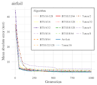
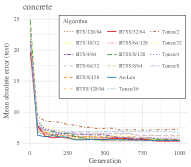
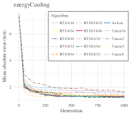
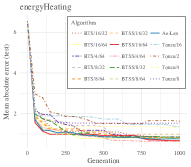
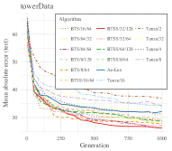
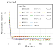
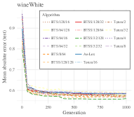
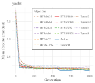
Figure 1. Curves showing the MMAE on the test set.

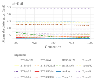
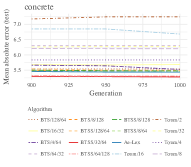
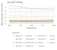
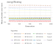
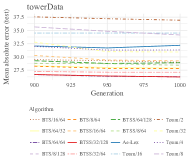
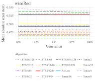
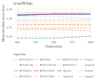
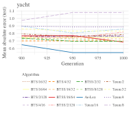
Figure 2. Curves zoomed on the last 100 generations showing the MMAE on the test set.

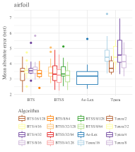
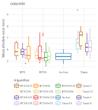
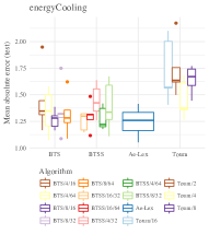
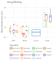
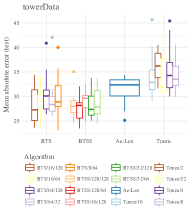
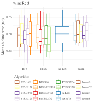
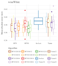
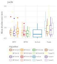
Figure 3. Boxplots of the MAE on the test set.

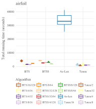
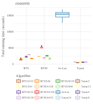
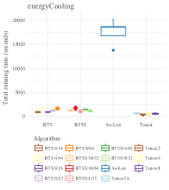
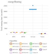
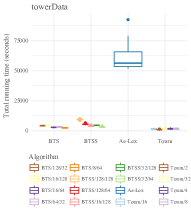
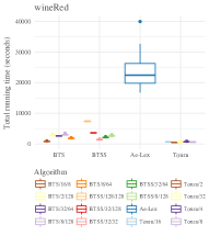
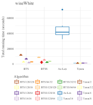
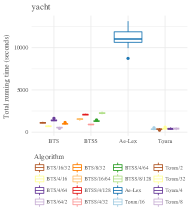
Figure 4. Boxplots of the total running time in seconds.

Table 3. Quality and speedup. Wilcoxon-Rank sum test ($\alpha=5\%$) with Ae-Lex as baseline where symbol ’-’ means the method had lower MMAE than Ae-Lex, and ’+’ means the opposite. We compare only to the Ae-Lex (the baseline).

airfoil			concrete			energyCooling			energyHeating
Algorithm	MMAE	Speedup	Algorithm	MMAE	Speedup	Algorithm	MMAE	Speedup	Algorithm	MMAE	Speedup
Ae-Lex	$3.129$	1.00	Ae-Lex	$5.424$	1.00	Ae-Lex	$1.279$	1.00	Ae-Lex	$0.733$	1.00
BTSS/8/128	$3.274$	11.30	BTSS/64/32	$5.223$	7.76	BTSS/4/64	$1.189$	12.73	BTSS/4/64	$0.689$	13.89
BTSS/32/64	$3.279$	12.61	BTSS/64/128	$5.234$	3.05	BTS/8/64	$1.237$	11.23	BTSS/16/64	$0.697$	11.69
BTSS/8/64	$3.286$	16.22	BTSS/8/64	$5.337$	9.79	BTSS/16/32	$1.258$	14.18	BTS/16/32	$0.740$	15.13
BTSS/32/128	$3.334^{+}$	7.55	BTSS/8/128	$5.350$	6.08	BTS/4/64	$1.267$	11.61	BTS/8/64	$0.769$	12.44
BTSS/4/128	$3.377^{+}$	11.46	BTSS/4/128	$5.370$	6.48	BTS/8/16	$1.313$	20.12	BTSS/8/64	$0.777$	12.83
BTS/4/32	$3.467^{+}$	20.77	BTS/8/128	$5.444$	5.27	BTS/4/16	$1.355$	19.22	BTS/4/64	$0.785$	13.04
BTS/8/64	$3.467^{+}$	14.30	BTS/8/64	$5.583$	8.72	BTSS/8/32	$1.370$	17.16	BTSS/16/32	$0.820$	17.64
BTS/16/128	$3.526^{+}$	8.10	BTS/2/64	$5.745^{+}$	9.85	BTS/8/32	$1.411$	14.82	BTS/8/32	$0.856^{+}$	19.32
BTS/4/16	$3.557^{+}$	25.84	BTS/64/32	$5.841^{+}$	6.96	BTSS/16/64	$1.423$	10.48	BTSS/8/32	$0.856^{+}$	19.86
BTS/8/16	$3.626^{+}$	23.63	BTS/16/32	$5.883^{+}$	11.53	BTSS/4/32	$1.571^{+}$	18.80	BTS/16/64	$0.940^{+}$	10.44
towerData			wineRed			wineWhite			yacht
Algorithm	MMAE	Speedup	Algorithm	MMAE	Speedup	Algorithm	MMAE	Speedup	Algorithm	MMAE	Speedup
Ae-Lex	$32.423$	1.00	Ae-Lex	$0.472$	1.00	Ae-Lex	$0.603$	1.00	Ae-Lex	$0.686$	1.00
BTS/16/128	$27.358^{-}$	13.29	BTS/8/128	$0.449$	7.58	BTSS/128/128	$0.524^{-}$	4.79	BTS/64/2	$0.648$	20.78
BTSS/32/128	$27.505^{-}$	12.32	BTSS/32/128	$0.463$	6.22	BTSS/64/64	$0.529^{-}$	11.57	BTS/16/32	$0.697$	10.05
BTSS/32/64	$27.843^{-}$	18.35	BTS/8/64	$0.464$	12.26	BTS/64/32	$0.550^{-}$	14.41	BTSS/16/64	$0.702$	7.06
BTSS/128/128	$28.036^{-}$	5.95	BTS/32/64	$0.467$	8.59	BTSS/128/16	$0.560^{-}$	17.79	BTS/4/16	$0.708$	16.24
BTS/64/32	$28.266^{-}$	18.48	BTSS/8/128	$0.468$	8.67	BTSS/128/64	$0.570^{-}$	8.16	BTSS/4/128	$0.709$	5.30
BTSS/128/64	$28.275^{-}$	10.23	BTSS/128/128	$0.480$	3.04	BTS/128/16	$0.574^{-}$	16.81	BTS/4/64	$0.729$	7.95
BTS/8/64	$28.826^{-}$	23.83	BTSS/32/32	$0.481$	15.90	BTS/128/64	$0.592^{-}$	6.36	BTSS/4/32	$0.759$	12.26
BTS/16/64	$29.224^{-}$	19.91	BTSS/32/64	$0.503$	10.63	BTS/128/128	$0.593^{-}$	3.60	BTSS/4/64	$0.759$	8.41
BTSS/16/128	$29.594^{-}$	14.90	BTS/2/128	$0.505$	8.14	BTSS/32/32	$0.594^{-}$	20.05	BTSS/8/128	$0.765$	4.93
BTS/128/32	$30.142$	13.49	BTS/16/8	$0.558$	27.11	BTS/16/16	$0.611$	24.86	BTS/8/32	$0.870$	11.34

Thus, BTS and BTSS are shown to achieve similar if not superior performance to Ae-Lex. Interestingly, BTS and BTSS are based on a simpler computation which allows it to reach speed-ups of circa $25$ (Table 5 and Figure 4). This speedup derives from the fact that both BTS and BTSS behave similarly to tournament selection and therefore have a lower computation complexity than Ae-Lex.

In Figure 5, the frequency for the top five configurations are displayed. Small batches that are big enough to decrease randomness but small enough to allow for specialization are usually among the best configurations. Moreover, batches that change constantly create selection pressures that vary from generation to generation, decreasing the effects of any specialization that could take place. This explains the slight improvement of BTS over BTSS. In other words, in comparison with shuffled batches (BTSS), batches that are ordered by difficulty (BTS) tend to keep batches without changes throughout generations. This allows for better specializations. Having said that, the probability distribution of batches is constant in BTSS and therefore there is a number of batch permutations that are more probable than others. Therefore, BTSS also allows for certain specializations to appear.

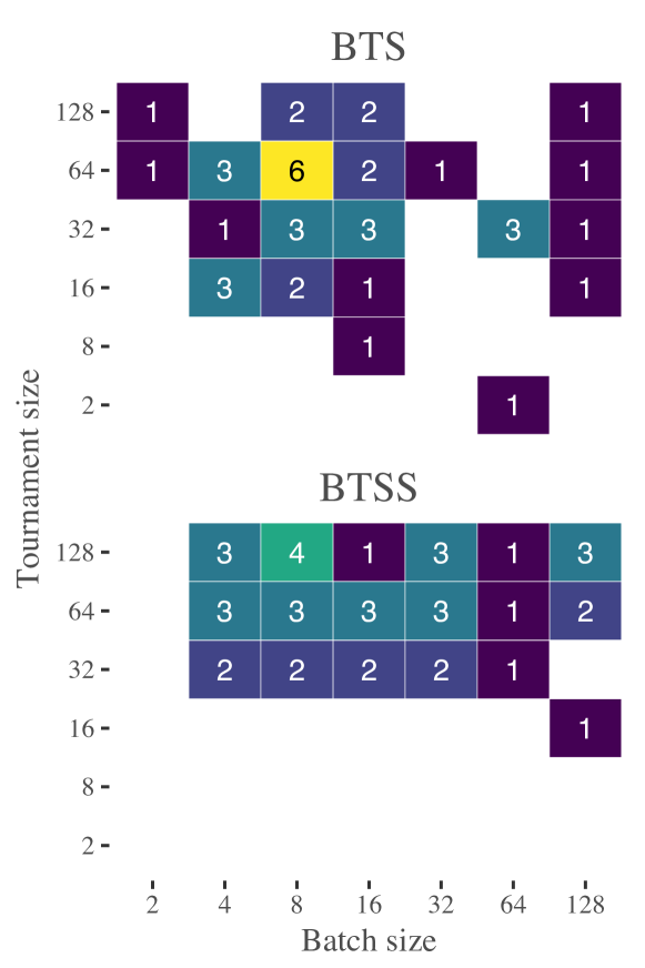
Figure 5. Frequency for configurations that reside in the top-five for any of the data sets. Notice that we do not depict a rank here but how many times each configuration was among the best. A blank cell means that this configuration was not in the top-five for any of the data sets.

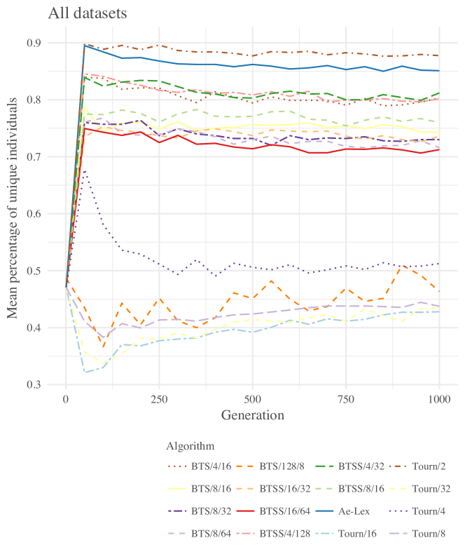
Figure 6. Diversity of the population over the generations for the top-five overall configuration.

4.5.2. Diversity Analysis

In this paper, we are using a straightforward diversity measure that considers only the individual’s value (its fitness), not its structure. Thus, if two completely different individuals provide the same result (fitness) they are considered equal. Here we are interested in how the individuals perform, not how they look like. Structural analysis can be done in a future work.

Diversity in both lexicase and tournament selection depend on how competition takes place and both batch as well as tournament size play important roles. To analyze deeply the diversity behavior, we did some experiments comparing some of the best performing algorithms in terms of diversity (Figure 6). It is clear that pure tournaments do not reach the diversity of Ae-Lex. This happens because in tournaments generalists are usually favoured. Which causes the entire population to be similar (Tourn/2 is an exception because the size of the tournament is small enough to make the influence of the tournament almost zero. Consequently, selection becomes mostly random. This naturally allows for a higher diversity with a trade-off on quality of solutions). Regarding Ae-Lex and BTS/BTSS, around $5$ layers of diversity can be observed in Figure 6: $Ae-Lex>BTSS4/32,BTSS4/128,BTS4/16>BTSS8/16,BTS8/16>BTS8/32,BTSS16/32,BTS8/64,BTSS16/64>BTS128/8$. This sequence can be explained by recalling the roles of both batch size and tournament size. In one hand, batch size controls the overall competition scenario. When batch size is big, batches will tend to have a similar distribution, reducing the niching effect and consequently favouring general solutions. Small batches have the opposite effect. Since general solutions are similar by definition, the overall diversity of the population decreases. This explains why bigger batch sizes result in less diversity. In fact, all the $5$ layers shown in Figure 6 respect this sequence.

Regarding the tournament size, it does not influence diversity strongly. Notice that even if they allow some sub-optimal individuals to survive, these sub-optimal individuals have a small chance of surviving the following generation. Thus, tournament can be seen mostly as an approximation to the maximum function of selecting the optimum individuals. Having said that, very small tournament sizes may cause generalists to survive even in small batches. This happens because the chance of a specialist individual being chosen to compete in a favourable batch is smaller. Therefore, general solutions which perform better overall would be favoured. This partially explains the diversity of BTS128/8 but the batch size of $128$ is also strongly affecting the diversity towards general solutions. Moreover, Figure 6 demonstrates that tournament size of $16$, $32$ and $128$ achieve similar diversity.

In summary, BTS and BTSS show that the use of batches can achieve a diversity that rivals Ae-Lex while being efficient. Canonical tournament selection runs fail to achieve the level of diversity which further explains their poor solution quality.

4.5.3. Batches and Ordered Test Cases

Surprisingly, both BTS and BTSS do not use ordered test cases but batches while achieving similar accuracy and diversity to Ae-Lex. Batches may have a totally different characteristic but both batches and test sequences allow for specialization to happen. In test sequences, order of test cases creates a priority which fosters specialization. In batches, groups of test cases define niches in which specialization happens.

5. On the Survival of Specialists

In Nature, there is no global fitness function. Geography plays a big role in dividing species into niches. And even in narrow places, species find ways to survive which differ from each other, creating in fact different fitness functions. Diversity is itself a byproduct of specialization caused by natural multi-objectivization. In fact, diversity measures within a single population have already been shown to not help evolution, causing a deleterious conflict between diversity and selection pressure that can only be solved with sub-populations and multiple objectives (Vargas et al., 2015).

In BTS and BTSS, similarly to Ae-Lex, diversity is achieved through specialization and multi-objectivization. Batches can be seen as different fitness functions (multi-objectivization) which create different selection pressures, allowing for diversity to appear naturally. Specialization seems to arrive as a consequence of batches with few changes throughout generations.

6. Conclusions

In this paper, we proposed the BTS, which combines the ability of lexicase selection to provide accurate solutions with the computational complexity of simple tournament selection. Interestingly, BTS achieves with batches a diversity similar to lexicase selection, showing that batches are indeed very similar in behavior to the ordering of test cases.

We argued that the similarity here derives from the fact that both BTS and lexicase selection foster specialization of individuals. In fact, fitness differs from batch to batch and therefore it can be said that different fitness measurements take place within a population. Consequently, BTS allows for multi-objectivization to appear, increasing diversity and driving specialization forward.

In summary, this work shows the following:

• Up to $25$ Times Speed Up With Similar Performance - BTS and BTSS provided a speed up of up to $25$ times when compared to Ae-Lex. This is a consequence of BTS and BTSS still having the computational complexity of tournament selection while having the accuracy of Ae-Lex.

• The Similarity Between Batches and Ordered Test Cases - The tests show that batches have a similar behavior to ordered test cases although the principle behind their mechanisms are completely different. This reveals that the main reason for Lexicase’s success may not be the ordered test cases but a more general principle which can be achieved in different ways.

• The Specialization and Multi-objectivization Hypothesis - This work sheds light on the inner workings of lexicase selection by creating an algorithm with similar behavior through a completely different mechanism. In fact, the similarity can be seen not only in terms of accuracy but also of diversity, demonstrating that the main principle behind Lexicase is conserved.

In summary, we propose an algorithm that can rival the state-of-the-art algorithms in performance while being one order of magnitude faster. Moreover, investigations into the diversity and overall performance of the proposed algorithms show a surprising similarity to lexicase selection, shedding light on the main principle behind Lexicase’s success.

- (1)
- Goldberg and Deb (1991) David E Goldberg and Kalyanmoy Deb. 1991. A comparative analysis of selection schemes used in genetic algorithms. In Foundations of Genetic Algorithms. Vol. 1. Elsevier, 69–93.
- Helmuth and Spector (2015) Thomas Helmuth and Lee Spector. 2015. General program synthesis benchmark suite. In Proceedings of the 2015 Annual Conference on Genetic and Evolutionary Computation. ACM, 1039–1046.
- Helmuth et al. (2015) Thomas Helmuth, Lee Spector, and James Matheson. 2015. Solving uncompromising problems with lexicase selection. IEEE Transactions on Evolutionary Computation 19, 5 (2015), 630–643.
- Jin (2011) Yaochu Jin. 2011. Surrogate-assisted evolutionary computation: Recent advances and future challenges. Swarm and Evolutionary Computation 1, 2 (2011), 61–70.
- Krawiec and Liskowski (2015) Krzysztof Krawiec and Paweł Liskowski. 2015. Automatic derivation of search objectives for test-based genetic programming. In European Conference on Genetic Programming. Springer, 53–65.
- La Cava et al. (2016) William La Cava, Lee Spector, and Kourosh Danai. 2016. Epsilon-lexicase selection for regression. In Proceedings of the Genetic and Evolutionary Computation Conference 2016. ACM, 741–748.
- Liskowski et al. (2015) Pawel Liskowski, Krzysztof Krawiec, Thomas Helmuth, and Lee Spector. 2015. Comparison of semantic-aware selection methods in genetic programming. In Proceedings of the Companion Publication of the 2015 Annual Conference on Genetic and Evolutionary Computation. ACM, 1301–1307.
- Miller et al. (1995) Brad L Miller, David E Goldberg, et al. 1995. Genetic algorithms, tournament selection, and the effects of noise. Complex Systems 9, 3 (1995), 193–212.
- Nordin and Banzhaf (1997) Peter Nordin and Wolfgang Banzhaf. 1997. An on-line method to evolve behavior and to control a miniature robot in real time with genetic programming. Adaptive Behavior 5, 2 (1997), 107–140.
- Nordin et al. (1998) Peter Nordin, Wolfgang Banzhaf, and Markus Brameier. 1998. Evolution of a world model for a miniature robot using genetic programming. Robotics and Autonomous Systems 25, 1-2 (1998), 105–116.
- Oliveira et al. (2016) Luiz Otavio VB Oliveira, Fernando EB Otero, and Gisele L Pappa. 2016. A dispersion operator for geometric semantic genetic programming. In Proceedings of the Genetic and Evolutionary Computation Conference 2016. ACM, 773–780.
- Oltean and Grosan (2003) Mihai Oltean and C. Grosan. 2003. A Comparison of Several Linear Genetic Programming. TECHNIQUES, COMPLEX-SYSTEMS 14 (2003), 282–311.
- Spector (2012) Lee Spector. 2012. Assessment of problem modality by differential performance of lexicase selection in genetic programming: a preliminary report. In Proceedings of the 14th annual Conference Companion on Genetic and Evolutionary Computation. ACM, 401–408.
- Vargas et al. (2015) Danilo Vasconcellos Vargas, Junichi Murata, Hirotaka Takano, and Alexandre Cláudio Botazzo Delbem. 2015. General sub-population framework and taming the conflict inside populations. Evolutionary Computation 23, 1 (2015), 1–36.
- Vargas et al. (2013) Danilo Vasconcellos Vargas, Hirotaka Takano, and Junichi Murata. 2013. Self organizing classifiers and niched fitness. In Proceedings of the fifteenth annual Conference on Genetic and Evolutionary Computation Conference. ACM, 1109–1116.