Distribution of velocities in an avalanche, and related quantities: Theory and numerical verification

Abstract

We study several probability distributions relevant to the avalanche dynamics of elastic interfaces driven on a random substrate: The distribution of size, duration, lateral extension or area, as well as velocities. Results from the functional renormalization group and scaling relations involving two independent exponents, roughness $\zeta$, and dynamics $z$, are confronted to high-precision numerical simulations of an elastic line with short-range elasticity, i.e. of internal dimension $d=1$. The latter are based on a novel stochastic algorithm which generates its disorder on the fly. Its precision grows linearly in the time discretization step, and it is parallelizable. Our results show good agreement between theory and numerics, both for the critical exponents as for the scaling functions. In particular, the prediction ${\sf a}=2-\frac{2}{d+\zeta-z}$ for the velocity exponent is confirmed with good accuracy.

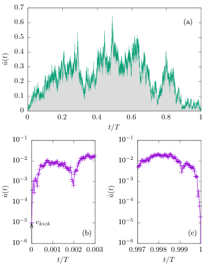
Figure 1: (a) The velocity as a function of time $t$ for one avalanche of duration $T$. (Parameters are $T=26.2$, $A=10$, $L=64$, $m=1$). Zooms of the departure (b), and ending (c) of the avalanche. The arrow in (b) indicates the magnitude $v_{\rm kick}$ of the uniform velocity kick triggering the avalanche.

Introduction

Disordered systems, when driven slowly or via a small kick, do not respond smoothly, but in a bursty way. An example are elastic manifolds, or more specifically elastic strings, subject to a random potential. An example for the global velocity as function of time is shown on figure 1. At $t=0$, the system received a small kick. The velocity as a function of time $t$ then performs a random walk, which terminates at a precise moment in time. Driving the system adiabatically slowly, it is at rest for most of the time, interceded with jerky motion as the one shown on figure 1. Each such event is called an avalanche. Avalanches are ubiquitous, found in earthquakes in geoscience GutenbergRichter1956 , Barkhausen noise Barkhausen1919 ; CizeauZapperiDurinStanley1997 in dirty disordered magnets, contact-lines on a disordered substrate LeDoussalWieseMoulinetRolley2009 , and many more.

The theory has been developed for many years, starting with phenomenological and mean-field arguments BuldyrevBarabasiCasertaHavlinStanleyVicsek1992 ; DSFisher1998 . In the context of magnets, a more systematic approach was proposed by Alessandro, Beatrice, Bertotti, and Montorsi (ABBM) AlessandroBeatriceBertottiMontorsi1990b ; AlessandroBeatriceBertottiMontorsi1990 , who reduced the equation of motion for a magnetic domain wall to a single degree of freedom, subject to a random force modeled as a random walk. It was only realized later LeDoussalWiese2011a that the Brownian force model (BFM) is the correct mean-field theory for avalanche dynamics. In contrast to the ABBM or similar mean-field models, which have a single degree of freedom, the BFM is an extended model, in which each degree of freedom, i.e. each piece of the elastic manifold, sees an independent random force, which itself is a random walk. In LeDoussalWiese2011a it was shown that its center of mass is the same stochastic process as the single degree of freedom of the ABBM model.

The BFM is the starting point for a field theory of elastic manifolds subject to short-ranged disorder. It allows to calculate a plethora of observables beyond pure scaling exponents, as e.g. the full size LeDoussalWiese2011b ; LeDoussalWiese2009a ; LeDoussalWiese2008c distribution, the velocity distribution LeDoussalWiese2012a ; LeDoussalWiese2011a , and the temporal DobrinevskiLeDoussalWiese2011b ; DobrinevskiLeDoussalWieseTBP or spatial shape ThieryLeDoussalWiese2015 ; DelormeLeDoussalWiese2016 ; AragonKoltonDoussalWieseJagla2016 ; ZhuWiese2017 of an avalanche.

In this letter we study numerically, and compare to field theory, the distributions of the duration $T$ of an avalanche, its size $S=\int_{0}^{T}\dot{u}(t)\mathrm{d}t$, its velocity $\dot{u}$, and extension $\ell$. We briefly review the corresponding scaling relations, and then confront them to large-scale numerical simulations. The latter has been possible through the development of a novel powerful algorithm which generates its disorder on the fly by accurately solving an extension of the BFM to incorporate short-ranged disorder.

	$P(S)$	$P(T)$	$P(\dot{u})$	$P(V)$
	$S^{-\tau}$	$T^{-\alpha}$	$\dot{u}^{-\sf a}$	$V^{-{\sf k}_{V}}\rule[-4.30554pt]{0.0pt}{15.0694pt}$
SR elasticity	$\tau=2-\frac{2}{d+\zeta}$	$\alpha=1+\frac{d-2+\zeta}{z}$	${\sf a}=2-\frac{2}{d+\zeta-z}$	${\sf k}_{V}=2-\frac{2-\zeta}{d}\rule[-6.45831pt]{0.0pt}{19.37494pt}$
LR elasticity	$\tau=2-\frac{1}{d+\zeta}$	$\alpha=1+\frac{d-1+\zeta}{z}$	${\sf a}=2-\frac{1}{d+\zeta-z}$	${\sf k}_{V}=2-\frac{1-\zeta}{d}\rule[-6.45831pt]{0.0pt}{19.37494pt}$

	$d$	$\zeta$	$z$	$\tau$	$\alpha$	${\sf a}$	$\gamma$	${\sf k}_{V}$
	$1$	$5/4$	$10/7$	$10/9$	$47/40$	$-10/23$	$1.57$	1.25
SR	$2$	$0.75$	$1.56$	$1.27$	$1.48$	$0.32$	$1.76$	1.38
	$3$	$0.35$	$1.75$	$1.40$	$1.77$	$0.75$	$1.91$	1.45
LR	$1$	$0.39$	$0.77$	$1.28$	$1.51$	$0.39$	$1.81$	1.39

Table 1: Left: Scaling relations. Right: Critical exponents obtained via the scaling relations using standard values for $\zeta$ and $z$ LeschhornNattermannStepanowTang1997 ; DuemmerKrauth2005 ; FerreroBustingorryKolton2012 ; GrassbergerDharMohanty2016 .

Definition of the model.

Consider the over-damped equation of motion for a manifold in a random-field environment,

$$\partial_{t}u_{x,t}=\partial_{x}^{2}u_{x,t}+F(x,u_{x,t})+m^{2}(w_{t}-u_{x,t})\ .$$ (1)

The manifold is trapped in a harmonic potential of width $m^{2}$, and position $w_{t}$. The well is moved slowly, either via $w_{t}=vt$ in the limit $v\to 0^{+}$ (constant velocity driving), or by augmenting $w$ by a small amount $\delta w$ at discrete times $t$ (kick driving). $F$ is a short-ranged correlated random force, which will be specified below. Eq. (1) provides a well-defined framework to study avalanches, both in field theory LeDoussalWiese2011a ; DobrinevskiLeDoussalWiese2011b ; LeDoussalWiese2012a ; DobrinevskiLeDoussalWiese2014a ; DobrinevskiPhD ; DobrinevskiLeDoussalWieseTBP , as for simulations RossoLeDoussalWiese2006a ; RossoLeDoussalWiese2009a ; KoltonSchehrLeDoussal2009 ; FerreroBustingorryKolton2013 ; FerreroBustingorryKoltonRosso2013 ; KoltonJagla2018 ; CaoBouzatKoltonRosso2018 . Indeed, the velocity as a function of time performs a burst-like evolution, with a well-defined beginning and end, see figure 1, separated by periods without activity (not shown).

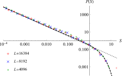
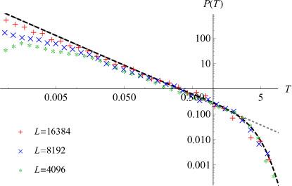
Figure 2: Left: The rescaled distribution of size $P(S)$. To avoid system-spanning avalanches, the ratio $Lm=10$ is kept fixed. The black dashed line is the 1-loop result (12) of Ref. LeDoussalMiddletonWiese2008 , the gray dotted line the pure power law. Right: ibid for the duration distribution $P(T)$. The analytical result is given in Eqs. (3.113)-(3.116) of Ref. DobrinevskiPhD and in Ref. DobrinevskiLeDoussalWieseTBP .

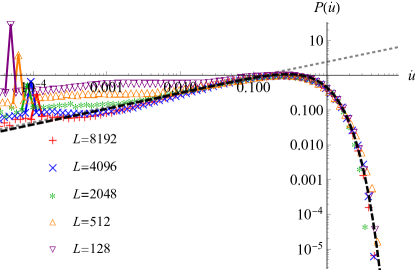
Figure 3: The center-of mass velocity distribution $P(\dot{u})$. The weight of the peak at $\dot{u}=v_{\rm kick}$ is $\frac{\delta t}{\left<T\right>}\sim L^{-z}\sim m^{z}$, where $T$ is the duration of an avalanche and $\delta t$ the time discretization step. The analytic result (black dashed line) is from Eq. (385) of Ref. LeDoussalWiese2012a , the dotted gray line the pure power law $P(\dot{u})\sim u^{{\sf a}}$.

Scaling relations.

The theory of the depinning transition of interfaces NattermannShort ; NarayanDSFisher1992b ; NarayanDSFisherInterface ; LeschhornNattermannStepanowTang1997 ; ChauveLeDoussalWiese2000a ; ChauveLeDoussalWieseDepLong introduces two independent critical exponents, the roughness exponent $\zeta$, and the dynamic exponent $z$. Within the field theory developed in LeDoussalWiese2011a ; DobrinevskiLeDoussalWiese2011b ; LeDoussalWiese2012a ; DobrinevskiLeDoussalWiese2014a ; DobrinevskiPhD ; DobrinevskiLeDoussalWieseTBP no independent exponent is required to describe avalanches. As a consequence, their exponents are given by scaling relations, together with the requirement of the existence of a massless field theory DobrinevskiLeDoussalWiese2014a , a generalization of the arguments of Ref. NarayanDSFisher1992b . Consider the PDF $P_{\delta w}(S)$ of the total size $S$ of the avalanche following a small kick $\delta w$. Its large-size cutoff $S_{m}\sim m^{-(d+\zeta)}$ is defined through the ratio of its first two moments LeDoussalWiese2008c

$$S_{m}=\frac{\left<S^{2}\right>}{2\left<S\right>}\ .$$ (2)

The PDF reads, for $S$ larger than a microscopic cutoff

$$P_{\delta w}(S)\simeq\frac{\left<S\right>}{S_{m}^{2}}p(S/S_{m})\quad,\quad\left<S\right>=\delta wL^{d}\ ,$$ (3)

where $p(s)$ is a universal scaling function with $p(s)\sim s^{-\tau}$ at small $s$, defining the size exponent $\tau$. Existence of a massless field theory imposes that the avalanche density per unit applied force, $\rho_{f}(S)=\lim_{\delta w\to 0}\frac{1}{m^{2}\delta w}P_{\delta w}(S)$ has a finite limit for $m\to 0$. This requires $m^{-2}S_{m}^{\tau-2}$ to be independent of $m$ at small $m$, hence $\tau=2-\frac{2}{d+\zeta}$, recovering the value of Narayan and Fisher NarayanDSFisher1992b . The exponents for the avalanche duration $T$, or lateral size $\ell$ are then obtained by writing $P_{\delta w}(S)\mathrm{d}S=P_{\delta w}(T)\mathrm{d}T$, and using the appropriate scaling relations between $S$, $m$ and $T$, leading to the results in the Table 1, where numerical values are given as well. We also consider the (spatially integrated) velocity at time $t$ after the kick, $\dot{u}(t)=\int\mathrm{d}^{d}x\,\partial_{t}u_{x,t}$. The PDF of the total velocity $\dot{u}=\dot{u}(t)$ is obtained by considering many successive kicks and sampling the time $t$ uniformly. Its associated density is $\rho_{f}(\dot{u})\sim\int\mathrm{d}t\,\rho_{f}\big{(}\dot{u}(t)\big{)}$. By scaling it takes at small $\dot{u}$ the form $\rho_{f}(\dot{u})=\frac{L^{d}}{m^{2}v_{m}^{2}}(v_{m}/\dot{u})^{\sf a}$ where ${\sf a}$ is the velocity exponent, $v_{m}=S_{m}/\tau_{m}$ and $\tau_{m}\sim m^{-z}$ is the large time cutoff. Requirement of a massless limit implies

$${\sf a}=2-\frac{2}{d+\zeta-z}\ ,$$ (4)

a main prediction of Ref. DobrinevskiLeDoussalWiese2014a , in agreement with the $\varepsilon$ expansion of Ref. LeDoussalWiese2012a , and which we test numerically below.

The algorithm: Theory.

The equation of motion of an elastic manifold due to short-ranged disorder-forces can be generated by the following set of equations (with an arbitrary constant $A$) DobrinevskiPhD ; LeDoussalWiese2014a

$$\partial_{t}{\cal F}_{x,t}=-A{\cal F}_{x,t}{\dot{u}_{x,t}}+\sqrt{2A\dot{u}_{x,t}}\;\xi(x,t)\ ,$$ (5)

$$\partial_{t}\dot{u}_{x,t}=\partial_{x}^{2}\dot{u}_{x,t}+\partial_{t}{\cal F}_{x,t}+m^{2}(v-\dot{u}_{x,t})\ ,~{}~{}~{}~{}~{}~{}$$ (6)

$$\left<\xi(x,t)\xi(x^{\prime},t^{\prime})\right>=\delta(x-t^{\prime})\delta(t-t^{\prime})\ .$$ (7)

Rewriting $F_{x,t}$ as a function of $x$ and $u_{x,t}$, ${\cal F}_{x,t}\equiv F(x,u_{xt})$ yields for each $x$ an evolution equation of $F(x,u)$,

$$\partial_{u}{F}(x,u)=-A{F}(x,u)+\sqrt{2A}\;\eta(x,u)\ ,$$ (8)

$$\left<\eta(x,u)\eta(x^{\prime},u^{\prime})\right>=\delta(x-x^{\prime})\delta(u-u^{\prime})\ .$$ (9)

The solution to this equation is

$$\overline{{F}(x,u){F}(x^{\prime},u^{\prime})} = \delta(x-x^{\prime})\,\mathrm{e}^{-A|u^{\prime}-u|}\ .$$ (10)

We can read off the microscopic disorder force-force correlator

$$\Delta(u-u^{\prime})=\mathrm{e}^{-A|u^{\prime}-u|}\ .$$ (11)

It is short-ranged, and microscopically rough. The problem is how to solve efficiently the stochastic equations (5)-(6). Discretizing time in steps of size $\delta t$ yields

$$\dot{u}_{t+\delta t}-\dot{u}_{t} = {\cal F}_{t+\delta t}-{\cal F}_{t}+O(\delta t)$$ (12)

$$= \sqrt{2A\dot{u}_{t}\delta t}\,\xi_{t}+O(\delta t)\ ,$$

where $\xi_{t}$ is a normal-distributed Gaussian random variable with mean $\left<\xi_{t}\right>=0$, and variance $\left<\xi_{t}\xi_{t^{\prime}}\right>=\delta_{t,t^{\prime}}$. Since one is interested in the limit of $\delta t\to 0$, the appearance of $\sqrt{\delta t}$ in front of the noise term implies a rather slow convergence.

The algorithm: An Improved Solver.

The idea is to solve analytically the random process

$$\partial_{t}\dot{u}_{t}=\sqrt{2A\dot{u}_{t}}\,\xi(t)$$ (13)

with absorbing boundary conditions at $\dot{u}=0$ for a finite interval $\delta t$. Following DornicChateMunoz2005 , we first write the analytic solution of the corresponding Fokker-Planck equation

$$P(\dot{u},t) = \delta(\dot{u})\exp\left(-\frac{\dot{u}_{0}}{At}\right)$$ (14)

$$+\frac{\exp\left(-\frac{\dot{u}_{0}+\dot{u}}{At}\right)}{At}\sqrt{\frac{\dot{u}_{0}}{\dot{u}}}\,I_{1}\!\left(\frac{2\sqrt{\dot{u}_{0}\dot{u}}}{At}\right)\ ,~{}~{}~{}$$

where $I_{1}$ is the Bessel-$I$ function of the first kind. It can be reexpressed as a series

$$P(\dot{u},t)=\sum_{n=0}^{\infty}p_{n}\,\frac{1}{A\,t}P_{n}\!\left(\frac{\dot{u}}{At}\right)$$ (15)

with

$$p_{n} = \frac{\left(\frac{\dot{u}_{0}}{At}\right)^{n}\exp\left(-\frac{\dot{u}_{0}}{At}\right)}{n!}$$ (16)

$$P_{0}(y) = \delta(y)$$ (17)

$$P_{n}(y) = \frac{y^{n-1}\exp\left(-y\right)}{(n-1)!}\ ,\qquad n\geq 1\ .$$ (18)

The algorithm consists of two steps: First draw a random number $n$ from a Poisson distribution with parameter $\frac{\dot{u}_{0}}{At}$. In a second step draw a random number $y$ from a Gamma-distribution with the (previously determined) parameter $n$. This yields

$$\dot{u}_{t+\delta t}=\dot{u}_{t}+A\,y\,\delta t\ ,$$ (19)

to which have to be added the drift terms proportional to $\delta t$.

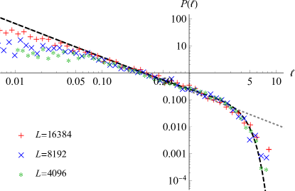
Figure 4: The distribution of lateral sizes $P(\ell)$. In absence of analytic results for the scaling function, we use the relation $P(\ell)\mathrm{d}\ell=P(S)\mathrm{d}S$, and $S=\ell^{{d+\zeta}}$ to infer the latter (black dashed line). A pure power law $P(S)\sim S^{{-\sf k}}$ is given as the gray dotted line.

Results: Size and duration distributions.

Our simulations are performed in dimension $d=1$. In figure 2, we report our findings for the avalanche-size and duration distributions, both known analytically from the $\varepsilon=4-d$ expansion LeDoussalWiese2008c ; DobrinevskiPhD ; DobrinevskiLeDoussalWieseTBP . The size distribution was also checked numerically RossoLeDoussalWiese2009a . One extends the definitions (2) and (3) to observables $\cal O$ such as the duration $T$ and extension $\ell$ (see below) by writing the PDF

$$P_{\delta w}({\cal O})=\frac{\left<{\cal O}\right>}{{\cal O}_{m}^{2}}p\!\left(\frac{{\cal O}}{{\cal O}_{m}}\right)\ ,$$ (20)

where ${\cal O}_{m}=\frac{\left<{\cal O}^{2}\right>}{2\left<\cal O\right>}$ is the characteristic large-scale cutoff and $p(x)$ is a universal function depending only on $d$ and ${\cal O}$, such that $\int_{0}^{\infty}\mathrm{d}x\,xp(x)=1$, $\int_{0}^{\infty}\mathrm{d}x\,x^{2}p(x)=2$. It is this function $p(x)$ which is plotted in figure 2 and 4 from our simulation, (denoted there by $P(x)$) and compared to its prediction from the $\varepsilon$ expansion (via an extrapolation to $\varepsilon=3$). While the scaling relations using $\zeta=5/4$ and $z=10/7$ predict a size exponent $\tau=1.11$ and a duration exponent $\alpha=1.17$, see table 1, our best fits are

$$\tau = 1.2\pm 0.2\ ,$$ (21)

$$\alpha = 1.1\pm 0.15\ .$$ (22)

Velocity distribution.

For the center of mass, the velocity distribution $P(\dot{u})$ is predicted to scale as

$$P(\dot{u})\sim\dot{u}^{-\sf a}\ ,$$ (23)

with a very large exponent ${\sf a}=1$ for the BFM and the ABBM model. On the other hand, the scaling relation ${\sf a}=2-\frac{2}{d+\zeta-z}$ predicts a negative exponent ${\sf a}=-0.45$ in dimension $d=1$, a quite dramatic deviation from the BFM and MF value. Remarkably, our simulations confirm this negative value, yielding

$${\sf a}=-0.45\pm 0.05\ .$$ (24)

Distribution of spatial extensions.

We finally consider the spatial extension $\ell$ of an avalanche. Using that $P(\ell)\mathrm{d}\ell=P(S)\mathrm{d}S$, and $S\sim\ell^{d+\zeta}$, we get

$$P(\ell)\sim\ell^{-\sf k}\ ,\qquad{\sf k}=d-1+\zeta~{}\stackrel{{\scriptstyle d=1}}{{-\!\!\!\longrightarrow}}~{}\zeta=1.25\ .$$ (25)

Our numerical data shown in Fig. 4 are in agreement with this scaling relation, yielding

$${\sf k}=1.25\pm 0.05\ .$$ (26)

In higher dimensions, the lateral extension of an avalanche is difficult to define, whereas its volume is well-defined. Using scaling arguments equating $P(V)\mathrm{d}V=P(S)\mathrm{d}S$, $S\sim\ell^{{d+\zeta}}$, and $V\sim\ell^{d}$ we find

$$P(V) \sim V^{-{\sf k}_{V}}\ ,$$ (27)

$${\sf k}_{V} = 2-\frac{2-\zeta}{d}\ .$$ (28)

Explicit values are given in table 1.

Conclusion.

In this letter, we confronted theoretical results for the distributions of avalanche size, duration, and velocity with numerical simulations. We confirm the theoretical results based on scaling arguments, and functional RG calculations to 1-loop order. Our comparison goes beyond scaling exponents, validating the full 1-loop scaling functions.

The model and algorithm proposed here can be generalized to arbitrary dimension and long-range interactions. It is computationally more demanding than the standard depinning model due to the presence of multiplicative noise, but it has the advantage that it allows one to compute more precisely the spatio-temporal extent of an avalanche and to reach the regime of adiabatic driving. It thus avoids the difficulties and artifacts associated with velocity thresholding. In addition, as its microscopic disorder has the statistics of a random walk at short scale, it is readily connected to the BFM model.

- (1) B. Gutenberg and C. F. Richter, Earthquake magnitude, intensity, energy, and acceleration, Bulletin of the Seismological Society of America 46 (1956) 105–145.
- (2) H. Barkhausen, Zwei mit Hilfe der neuen Verstärker entdeckte Erscheinungen, Phys. Z. 20 (1919) 401–403.
- (3) P. Cizeau, S. Zapperi, G. Durin and H. Stanley, Dynamics of a Ferromagnetic Domain Wall and the Barkhausen Effect, Phys. Rev. Lett. 79 (1997) 4669–4672.
- (4) P. Le Doussal, K.J. Wiese, S. Moulinet and E. Rolley, Height fluctuations of a contact line: A direct measurement of the renormalized disorder correlator, EPL 87 (2009) 56001, arXiv:0904.4156.
- (5) S.V. Buldyrev, A.-L. Barabasi, F. Caserta, S. Havlin, H.E. Stanley and T. Vicsek, Anomalous interface roughening in porous media: experiment and model, Phys. Rev. A 45 (1992) R8313–16.
- (6) D.S. Fisher, Collective transport in random media: From superconductors to earthquakes, Phys. Rep. 301 (1998) 113–150.
- (7) B. Alessandro, C. Beatrice, G. Bertotti and A. Montorsi, Domain-wall dynamics and Barkhausen effect in metallic ferromagnetic materials. II. Experiments, J. Appl. Phys. 68 (1990) 2908.
- (8) B. Alessandro, C. Beatrice, G. Bertotti and A. Montorsi, Domain-wall dynamics and Barkhausen effect in metallic ferromagnetic materials. I. Theory, J. Appl. Phys. 68 (1990) 2901.
- (9) P. Le Doussal and K.J. Wiese, Distribution of velocities in an avalanche, EPL 97 (2012) 46004, arXiv:1104.2629.
- (10) P. Le Doussal and K.J. Wiese, First-principle derivation of static avalanche-size distribution, Phys. Rev. E 85 (2011) 061102, arXiv:1111.3172.
- (11) P. Le Doussal and K.J. Wiese, Elasticity of a contact-line and avalanche-size distribution at depinning, Phys. Rev. E 82 (2010) 011108, arXiv:0908.4001.
- (12) P. Le Doussal and K.J. Wiese, Size distributions of shocks and static avalanches from the functional renormalization group, Phys. Rev. E 79 (2009) 051106, arXiv:0812.1893.
- (13) P. Le Doussal and K.J. Wiese, Avalanche dynamics of elastic interfaces, Phys. Rev. E 88 (2013) 022106, arXiv:1302.4316.
- (14) A. Dobrinevski, P. Le Doussal and K.J. Wiese, Non-stationary dynamics of the Alessandro-Beatrice-Bertotti-Montorsi model, Phys. Rev. E 85 (2012) 031105, arXiv:1112.6307.
- (15) T. Thiery, P. Le Doussal and K.J. Wiese, Spatial shape of avalanches in the Brownian force model, J. Stat. Mech. 2015 (2015) P08019, arXiv:1504.05342.
- (16) M. Delorme, P. Le Doussal and K.J. Wiese, Distribution of joint local and total size and of extension for avalanches in the Brownian force model, Phys. Rev. E 93 (2016) 052142, arXiv:1601.04940.
- (17) L.E. Aragon, A.B. Kolton, P. Le Doussal, K.J. Wiese and E. Jagla, Avalanches in tip-driven interfaces in random media, EPL 113 (2016) 10002, arXiv:1510.06795.
- (18) Z. Zhu and K.J. Wiese, The spatial shape of avalanches, Phys. Rev. E 96 (2017) 062116, arXiv:1708.01078.
- (19) T. Nattermann, et al., J. Phys. II (France) 2 (1992) 1483.
- (20) H. Leschhorn, T. Nattermann, S. Stepanow and L.-H. Tang, Driven interface depinning in a disordered medium, Annalen der Physik 509 (1997) 1–34, arXiv:cond-mat/9603114.
- (21) O. Dümmer and W. Krauth, Critical exponents of the driven elastic string in a disordered medium, Phys. Rev. E 71 (2005) 061601.
- (22) Ezequiel E. Ferrero, Sebastián Bustingorry and Alejandro B. Kolton, Non-steady relaxation and critical exponents at the depinning transition, Phys. Rev. E 87 (2013) 032122, arXiv:1211.7275.
- (23) P. Grassberger, D. Dhar and P. K. Mohanty, Oslo model, hyperuniformity, and the quenched Edwards-Wilkinson model, Phys. Rev. E 94 (2016) 042314.
- (24) A. Dobrinevski, P. Le Doussal and K.J. Wiese, Avalanche shape and exponents beyond mean-field theory, EPL 108 (2014) 66002, arXiv:1407.7353.
- (25) A. Rosso, P. Le Doussal and K.J. Wiese, Numerical calculation of the functional renormalization group fixed-point functions at the depinning transition, Phys. Rev. B 75 (2007) 220201, cond-mat/0610821.
- (26) A. Rosso, P. Le Doussal and K.J. Wiese, Avalanche-size distribution at the depinning transition: A numerical test of the theory, Phys. Rev. B 80 (2009) 144204, arXiv:0904.1123.
- (27) A.B. Kolton, G. Schehr and P. Le Doussal, Universal non-stationary dynamics at the depinning transition, Phys. Rev. Lett. 103 (2009) 160602, arXiv:0906.2494.
- (28) E. E. Ferrero, S. Bustingorry and A. B. Kolton, Nonsteady relaxation and critical exponents at the depinning transition, Phys. Rev. E 87 (2013) 032122.
- (29) E.E. Ferrero, S. Bustingorry, A.B. Kolton and A. Rosso, Numerical approaches on driven elastic interfaces in random media, Comptes Rendus Physique 14 (2013) 641 – 650.
- (30) A. B. Kolton and E. A. Jagla, Critical region of long-range depinning transitions, Phys. Rev. E 98 (2018) 042111.
- (31) Xiangyu Cao, Sebastian Bouzat, Alejandro B. Kolton and Alberto Rosso, Localization of soft modes at the depinning transition, Phys. Rev. E 97 (2018) 022118.
- (32) P. Le Doussal, A.A. Middleton and K.J. Wiese, Statistics of static avalanches in a random pinning landscape, Phys. Rev. E 79 (2009) 050101 (R), arXiv:0803.1142.
- (33) A. Dobrinevski, Field theory of disordered systems – avalanches of an elastic interface in a random medium, PhD Thesis, ENS Paris (2013), arXiv:1312.7156.
- (34) A. Dobrinevski, P. Le Doussal and K.J. Wiese, Avalanches beyond mean-field: durations and shape, to be published.
- (35) O. Narayan and D.S. Fisher, Critical behavior of sliding charge-density waves in 4-epsilon dimensions, Phys. Rev. B 46 (1992) 11520–49.
- (36) O. Narayan and D.S. Fisher, Phys. Rev. B 48 (1993) 7030.
- (37) D.S. Fisher, Interface fluctuations in disordered systems: expansion, Phys. Rev. Lett. 56 (1986) 1964–97.
- (38) P. Chauve, P. Le Doussal and K.J. Wiese, Renormalization of pinned elastic systems: How does it work beyond one loop?, Phys. Rev. Lett. 86 (2001) 1785–1788, cond-mat/0006056.
- (39) P. Le Doussal, K. J. Wiese, P. Chauve, 2-loop Functional Renormalization Group Theory of the Depinning Transition, arXiv:cond-mat/0205108, Phys. Rev. B 66 (2002) 174201.
- (40) P. Le Doussal and K.J. Wiese, An exact mapping of the stochastic field theory for Manna sandpiles to interfaces in random media, Phys. Rev. Lett. 114 (2014) 110601, arXiv:1410.1930.
- (41) I. Dornic, H. Chaté and M.A. Muñoz, Integration of Langevin equations with multiplicative noise and the viability of field theories for absorbing phase transitions, Phys. Rev. Lett. 94 (2005) 100601.