Few-body systems in Minkowski space: the Bethe-Salpeter Equation challenge

Abstract

Solving the homogeneous Bethe-Salpeter equation directly in Minkowski space is becoming a very alive field, since, in recent years, a new approach has been introduced, and the reachable results can be potentially useful in various areas of research, as soon as the relativistic description of few-body bound systems is relevant. A brief review of the status of the novel approach, which benefits from the consistent efforts of different groups, will be presented, together with some recent results

1 Introduction

A fully covariant and non perturbative description of a bound system, with and without spin degrees of freedom (dofs), represents a Holy Grail in different areas of research, as soon as relativistic effects become urgent for obtaining a reliable control of the dynamical evolution of the state. Indeed, a bound system has a unavoidably non perturbative nature, and if it is necessary a relativistic description, one keenly quests a suitable approach with the above mentioned features for tackling the issue. In view of this, the Bethe-Salpeter equation (BSE) in Minkowski space can play a role, since it was proposed by Salpeter and Bethe [1] within a fully field-theoretical and non perturbative framework (see Ref. [2] for a first review). In particular, the capability to offer a non perturbative description has to be ascribed to its-own structure, since the BSE for bound states is a homogeneous integral equation, and hence it is able to take into account all the infinite exchanges, needed to reproduce the bound-state pole (in the relevant Green’s function). Given such an attractive feature, the BSE has been actively studied, but the presence of many challenges related to, e.g., the need of kernels beyond the ladder one (see the next Section), the presence of self-energy and vertex corrections and, last but not least, the non trivial analytic structures of the BS amplitude (i.e. the solution of the BSE), has urged the introduction of wise mathematical trick, like the Wick rotation [3] and/or sharp approximations. As is well-known, very popular approaches to the BS formalism are based on the rotation to imaginary relative energy (see, e.g. Ref. [4] for an application to the deuteron) or on productive 3D-reductions of the BSE (see e.g., Ref. [5] for some introductory details), and they are devised for circumventing the issue of the cumbersome analytic structure in Minkowski momentum-space, related to the role of the relative energy (as well as the meaning of the relative time). There exist also covariant approximation of the BSE (see, e.g., Ref. [6] illustrating the covariant spectator model approach and Ref. [7] for the approach based on separable kernels), where some simplifying assumptions are introduced but still keeping safe the covariant nature of BSE. Till nineties, only one case was known to be exactly solved in Minkowski momentum-space, though with the interaction kernel in ladder approximation, namely the Wick-Cutkosky model [3, 8], which is composed by two massive scalars interacting through a massless scalar. In 1997, a new approach, based on i) the so-called Nakanishi Integral Representation (NIR) of the BS amplitude[9] and ii) its uniqueness, was introduced in order to successfully solve the ladder BSE governing a two-scalar system interacting through a massive scalar [10]. In particular, the emphasis of the work was on the calculations of both coupling constants needed for binding the system with assigned masses, and the so-called Nakanishi weight functions (see Sect. 3), rather than on the evaluation of the momentum distributions, so important in the phenomenological investigation of the inner dynamics of the bound systems. Nonetheless, Ref. [10] opened a new and attractive path, though the approach involved a lengthy algebraic manipulations. A substantial improvement was reached through the clever introduction [11] of the light-front (LF) framework (see e.g., Refs [12, 13] for detailed reviews). Indeed, by adopting LF variables, $x^{\pm}=x^{0}\pm x^{3}$ and ${\bf x}_{\perp}\equiv\{x^{1},x^{2}\}$, it is possible to simplify the treatment of the needed analytical integrations, extending the realm of application even including bound system with spin dofs [14, 15, 16], and, more important, a probabilistic framework can be established.

In Sects. 2 and 3 some snapshots on the Bethe-Salpeter equation and the Nakanishi integral representation of the BS amplitude will be presented, while Sect. 4 is devoted to the LF framework. Finally Sects. 5 and 6 contain some numerical results and perspectives, respectively

2 The Bethe-Salpeter equation in a nutshell

To briefly illustrate the main steps leading to the BSE, let us consider a simple two-scalar case (without antiparticles). The 4-point Green’s Function ($\phi_{i}$ are the scalar fields) is given by

$$G(x_{1},x_{2};y_{1},y_{2})=<0\,|\,T\{\phi_{1}(x_{1})\phi_{2}(x_{2})\phi_{1}^{+}(y_{1})\phi_{2}^{+}(y_{2})\}\,|\,0>~{}~{}~{},$$ (1)

and it fulfills the following inhomogeneous integral equation, sketched in Fig. 1,

$$G=G_{0}~{}+~{}G_{0}~{}{\cal I}~{}G$$ (2)

where $G_{0}$ is the product of four free propagators and ${\cal I}$ is the interaction kernel. It is given by the infinite sum of irreducible Feynman graphs, i.e. the ones that cannot be split into two lower order diagrams after cutting two internal particle lines and without touching the quantum lines [1]. The set of the irreducible diagrams up to the 6th power of the coupling constant are shown in Fig. 2. The first diagram, though it contains two interaction vertexes (hence, two coupling constants), generates the infinite ladder series, after iterating the integral equation in (2). The second diagram, that has four coupling constants, is the simplest crossed diagram. Finally, the last set of diagrams contain crossed diagram with 6 interaction vertexes. It is important to stress that each class of irreducible diagrams, contributing to the interaction kernel, in turn gives rise to an infinite series of diagrams by iteration. Such an observation allows us to anticipate that the solutions of the BSE corresponding to a truncated interaction kernel ${\cal I}$ contains however effects generated by an infinite set of powers of the coupling constant.

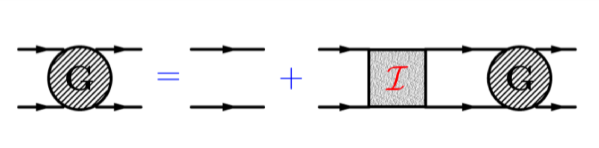
Figure 1: Pictorial representation of the inhomogeneous integral equation fulfilled by the four-leg Green’s function. The first irreducible diagrams contributing to the interaction kernel ${\cal I}$ are shown in Fig. 2.

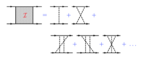
Figure 2: The lowest-order irreducible (see text) Feynman diagrams contributing to the interaction kernel of the integral equation for the four-leg Green’s function, Eq. (2). In a full theory, both interaction vertexes and propagators have to be properly dressed.

After properly inserting a complete 2-body Fock basis in $G(x_{1},x_{2};y_{1},y_{2})$, one can isolate the bound state contribution (assuming only one non-degenerate bound state, for the sake of simplicity) that manifests itself as a pole, in momentum space, i.e.

$$G(k,q;p)\Rightarrow G_{B}(k,q;p)\simeq{i\over(2\pi)^{-4}}~{}\frac{{\chi(k;p_{B})~{}\bar{\chi}(q;p_{B})}}{2\omega_{B}(p^{0}-\omega_{B}+i\epsilon)}$$ (3)

where $\omega_{B}=\sqrt{M^{2}_{B}+|{\bf p}|^{2}}$, $p_{B}^{\mu}\equiv\{\omega_{B},{\bf p}\}$ with $M_{B}$ the mass of the bound state (the adopted metric is $\{1,-1,-1,-1\}$), $k$ is the relative four-momentum of the pair and $\beta\equiv$ further quantum numbers. The function $\chi(k;p_{B})$ is called the BS amplitude, and describes the residue together with its conjugate (notice that the conjugate $\bar{\chi}$ is actually defined through Eq. (3) and involves the chronological product, to be carefully considered [2]). Unfortunately, the BS amplitude does not have a probabilistic interpretation, but one can profitably retrieve a probabilistic environment once the LF framework and the Fock expansion of the interacting two-body state is introduced (see Sect. 4). In conclusion, close to the bound-state pole, i.e. $p^{0}\to\omega_{B}=$ the Green’s function is approximated by

$$G\simeq~{}{i\over(2\pi)^{-4}}~{}\frac{{\chi(k;p_{B})~{}\bar{\chi}(q;p_{B})}}{2\omega_{B}(p^{0}-\omega_{B}+i\epsilon)}~{}+~{}regular~{}terms$$ (4)

By going through the following steps: i) insert the approximation (4) in both sides of $G=G_{0}+G_{0}~{}{\cal I}~{}G$, ii) multiply by $(p^{0}-\omega_{B})$ and iii) look close to the pole, one eventually gets the BSE, viz (see Fig. 3)

$$\chi(k;p_{B},\beta)=G_{0}(k;p_{B},\beta)~{}\int d^{4}k^{\prime}~{}{\cal I}(k,k^{\prime};p_{B})~{}\chi(k^{\prime};p_{B},\beta)$$ (5)

Figure 3: Pictorial representation of the Bethe-Salpeter integral equation for a bound system.

The normalization of the BS amplitude is given by (see Ref. [17], and Refs. [2, 18, 19] for further interesting issues on the BS norm)

$$\int{d^{4}q\over(2\pi)^{4}}\int{d^{4}k\over(2\pi)^{4}}~{}\bar{\chi}(q,p_{B})~{}\left.{\partial\over\partial p_{\mu}}\Bigl{[}G^{-1}_{0}(k,p)(2\pi)^{4}\delta^{4}(q-k)-i{\cal I}(q,k,p)\Bigr{]}\right|_{p^{2}=M^{2}_{B}}$$

$$\times~{}\chi(k,p_{B})=i2p^{\mu}_{B}$$ (6)

3 The Nakanishi integral representation and the BS Amplitude

In the sixties, Noburo Nakanishi [9, 20] proposed an integral representation of transition amplitudes (see Fig. 4), based on the parametric formula for the Feynman diagrams.

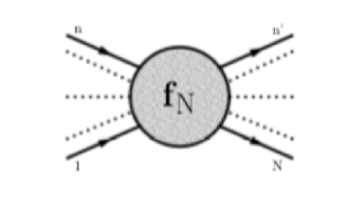
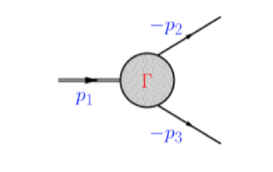
Figure 4: Left panel: transition amplitude with $N$ external legs. The bubble represents the infinite possible contributions, and the legs are represented just for enumerating the external momenta, but they do not indicate any external propagation. Right panel: the 3-leg transition amplitude, relevant for the application to the two-body Bethe-Salpeter amplitude (see text), the same previous caveat has to be applied to the external legs.

Within the perturbation theory for scalars, the transition amplitude with $N$ external legs, $f_{N}$, gets an infinite number of contributions, whose generic expression is given by

$$f_{\cal G}(p_{1},p_{2},...,p_{N})\propto~{}\prod_{i=1}^{k}\int d^{4}q_{i}~{}\frac{1}{(\ell_{1}^{2}-m_{1}^{2})(\ell_{2}^{2}-m_{2}^{2})~{}\dots~{}(\ell_{n}^{2}-m_{n}^{2})}$$ (7)

where $n$ indicates the total number of propagators, $k$ is the total number of loops ($\equiv$ number of integration variables), $\ell_{j}$ are the internal momenta, combinations of external momenta $p_{r}$ and loop ones $q_{i}$. The label ${\cal G}$ is a shorthand notation replacing $\{n,k\}$. By standard manipulations one can write

$$f_{\cal G}(\{p_{i}\})\propto~{}\prod_{j=1}^{n}\int_{0}^{1}d\alpha_{j}~{}\frac{\delta(1-\sum_{r}\alpha_{r})}{U(\{\alpha_{r}\})~{}\left[\sum_{r}\alpha_{r}m^{2}_{r}-\sum_{h}\eta_{h}(\{\alpha_{i}\})~{}s_{h}+i\epsilon\right]^{n-2k}}$$ (8)

where $\{\alpha_{i}\}$ are $n$ Feynman parameters, $\{s_{h}\}$ all the independent scalar products one can construct from the $N$ external legs with $1\leq h\leq N^{\prime}<N$, $\eta_{h}(\{\alpha_{r}\})$ and $U(\{\alpha_{r}\})$ are well-defined combinations of the Feynman parameters [20]. It is worth noticing that the dependence upon $\{n,k\}$ affects the denominator, and therefore each contribution to the total transition amplitude has its-own analytic structure. Nakanishi introduced a compact and elegant expression of the full $N$-leg amplitude $f_{N}(s)=\sum_{\cal G}~{}f_{\cal G}(s)$, by inserting in the generic contribution $f_{\cal G}$ the following identity

$$1\doteq\prod_{j=1}^{N^{\prime}}\int_{0}^{1}dz_{j}~{}\delta\left(z_{j}-\frac{\eta_{j}(\{\alpha_{i}\})}{\beta}\right)\int_{0}^{\infty}d\gamma~{}\delta\left(\gamma-\sum_{i}\frac{\alpha_{i}m_{i}^{2}}{\beta}\right)$$ (9)

where $\beta=\sum_{h}\eta_{h}(\{\alpha_{i}\})$ (see [20] for details). After integrating by parts $n-2k-1$ times the expression of $f_{\cal G}$, one gets from Eq. (8)

$$f_{\cal G}(\tilde{s})\propto~{}\prod_{j=1}^{N^{\prime}}\int_{0}^{1}dz_{j}\int_{0}^{\infty}d\gamma\frac{\delta(1-\sum_{j}z_{j})~{}\tilde{\phi}_{\cal G}(\vec{z},\gamma)}{{{(\gamma-\sum_{j}z_{j}~{}s_{j})}}}$$ (10)

where $\tilde{\phi}_{\cal G}(\vec{z},\gamma)$ is a proper weight function (that in this perturbative framework lives in the realm of the distribution functions), with $\vec{z}\equiv\{z_{1},z_{2},~{}\dots~{},z_{N^{\prime}}\}$ and $\tilde{s}\equiv\{s_{1},s_{2},~{}\dots~{},s_{N^{\prime}}\}$. Summarizing, the dependence upon the details of the diagram, i.e. $\{n,k\}$, moves from the denominator to the numerator. Hence, one has exactly the same formal expression for the denominator of any diagram ${\cal G}$.

The full $N$-leg transition amplitude is the sum of infinite diagrams ${\cal G}$ and it can be formally written as

$$f_{N}(\tilde{s})~{}=\sum_{\cal G}~{}f_{\cal G}(\tilde{s})\propto~{}\prod_{j=1}^{N^{\prime}}\int_{0}^{1}dz_{j}\int_{0}^{\infty}d\gamma\frac{\delta(1-\sum_{j}z_{j})~{}\phi_{N}(\vec{z},\gamma)}{(\gamma-\sum_{i}z_{i}~{}s_{i})}$$ (11)

where ${\phi}_{N}(\vec{z},\gamma)=\sum_{\cal G}\tilde{\phi}_{\cal G}(\vec{z},\gamma)$ is called a Nakanishi weight function (NWF). It is a real function, depending upon $N^{\prime}$ compact variables, $\vec{z}$, and one non compact, $\gamma$.

For the 3-leg transition amplitude, (cf the right panel in Fig. 4) after eliminating one compact variable and redefining the NWF, one reduces to

$$f_{3}(p^{2},k^{2},k\cdot p)=\int_{-1}^{1}dz\int_{0}^{\infty}d\gamma\frac{\pi_{3}(z,\gamma)}{\gamma+m^{2}-{p^{2}\over 4}-k^{2}-zk\cdot p-i\epsilon}$$ (12)

with $p=p_{1}+p_{2}$ and $k=(p_{1}-p_{2})/2$. Notice that $\phi_{3}$ is also known as the vertex function, $\Gamma$, for a scalar theory (N.B. for fermions one has to add spinor indexes). The expression holds at any order in perturbation-theory.

Once we put one leg on the mass shell, and we assume $\phi_{3}(z,\gamma)$ as an unknown functions, Eq. (12) becomes a natural choice as a trial function for obtaining actual solution of BSE for a two-scalar interacting system [9, 10, 11, 21]. The validation of this assumption, namely translating an expression formally elaborated within a perturbative framework to a non perturbative one, has been successfully obtained numerically, as discussed in what follows. This result should be not too much surprising if one takes into account the freedom associated to the NWF, that is the unknown to be determined.

A vertex function $f_{3}(k,p)$ with one leg on mass-shell is related to the BS amplitude $\chi$ by attaching propagators to the two external virtual legs, i.e. schematically: $\chi=G_{1}\otimes G_{2}\otimes f_{3}(\tilde{s})$ where $G_{i}$ are the propagators of the two particles. Finally one writes

$$\chi(k,p)=-i\int_{-1}^{1}dz^{\prime}\int_{-\infty}^{\infty}d\gamma^{\prime}\frac{g(z^{\prime},\gamma^{\prime};\kappa^{2})}{\left[\gamma^{\prime}+\kappa^{2}-k^{2}-z^{\prime}k\cdot p-i\epsilon\right]^{3}}$$ (13)

where $\kappa^{2}=m^{2}-M^{2}/4$, with $m$ the mass of the constituent scalars and $g(z^{\prime},\gamma^{\prime};\kappa^{2})$ indicates a NWF corresponding to a given mass $M$ of the interacting system. Indeed the lower extremum of $\gamma^{\prime}$ has to be put equal to zero, in order to avoid the spontaneous decay of the bound state.

4 Projecting BSE onto the hyper-plane $x^{+}=0$

As mentioned above, NIR yields the needed freedom for exploring non perturbative problems, once the NWFs are taken as unknown real quantities. Unfortunately, even adopting NIR, BSE still remains a highly singular integral equation in the Minkowski momentum space. The strategy adopted in Ref. [10] for obtaining actual solutions of the two-scalar homogeneous BSE, in ladder approximation, relied on the uniqueness of the NWF. Profitably, a more general approach was introduced by Carbonell and Karmanov [11, 14], that exploited the known analytic structure of the BS amplitude, once NIR is applied. Since the target is to determine the NWF, one can perform analytic integrations, to formally obtain a new integral equation, more suitable for the numerical treatment. The approach can be seen as a variant of the 3D reduction, but in this case the assumed expression of the BS amplitude in terms of NIR allows one the formally exact reconstruction of the full BS amplitude. In particular, in Ref. [11] an explicitly-covariant LF framework [13] was adopted, while the non-explicitly covariant version can be found in Refs. [22, 21]. It should be pointed out that the latter approach appears more suitable for isolating and mathematically treating further singularities one meets, particularly when the spin dofs are involved (see Refs. [15, 16]). In general, the LF approach allows one a simpler treatment of the analytic integration, since, e.g., double poles in the $k^{0}$ complex plane splits in pairs of single poles in the $k^{-}$ and $k^{+}$ complex planes.

In order to obtain an integral equation for the NWF more tractable from the numerical point of view (spin dofs lead to a system of integral equations), there is an illuminating step toward the final goal. One can recognize that within the LF framework a probabilistic interpretation is recovered by i) expanding the BS amplitude on a LF Fock basis, and ii) singling out the valence component. This is the amplitude of the Fock state with the lowest number of constituents, and it has (together with all the other amplitudes in the Fock expansion) the property to be invariant under LF-boost transformations (see Ref. [12]). In particular, the integral of the square modulus of the valence component gives the probability to find only two constituents in the interacting state. In the case of the non-explicitly covariant LF framework, the valence component is formally obtained by integrating the BS amplitude on $k^{-}=k^{0}-k^{3}$. Namely

$${\rm Valence~{}w.f.}=~{}\psi_{n=2}(\xi,k_{\perp})=~{}{p^{+}\over\sqrt{2}}~{}\xi~{}(1-\xi)\int{dk^{-}\over 2\pi}\chi(k,p)=$$

$$={1\over\sqrt{2}}\xi~{}(1-\xi)~{}\int_{0}^{\infty}d\gamma^{\prime}~{}{g(\gamma^{\prime},1-2\xi;\kappa^{2})\over[\gamma^{\prime}+k_{\perp}^{2}+\kappa^{2}+\left(2\xi-1\right)^{2}{M^{2}\over 4}-i\epsilon]^{2}}$$ (14)

where $\xi=(1-z)/2$, $M=2m-B$. with $B$ the binding energy. Notice that the above mathematical step is equivalent to make vanishing the relative LF-time $x^{+}$ in the BS amplitude in coordinate space (see, e.g.,[22, 21]), i.e. projecting the BS amplitude onto the hyperplane $x^{+}=0$. The above observations make attractive to study what happens when the $k^{-}$ integration is applied to both sides of BSE. As a matter of fact, on the lhs one has (a part trivial factors) the valence component that lives in a 3D space, and contains the NWF, while on the rhs one remains with a folding of the NWF with the so-called Nakanishi kernel, $V^{LF}(\alpha;\gamma,z;\gamma^{\prime},z^{\prime})$, viz

$${\rm valence~{}w.f.}~{}\propto~{}\int_{0}^{\infty}d\gamma^{\prime}\frac{g(\gamma^{\prime},z;\kappa^{2})}{[\gamma^{\prime}+\gamma+z^{2}m^{2}+(1-z^{2})\kappa^{2}-i\epsilon]^{2}}=$$

$$=\int_{0}^{\infty}d\gamma^{\prime}\int_{-1}^{1}dz^{\prime}~{}V^{LF}(\alpha;\gamma,z;\gamma^{\prime},z^{\prime})~{}~{}g(\gamma^{\prime},z^{\prime};\kappa^{2}).$$ (15)

where $\alpha$ is the coupling constant. N.B. $V^{LF}(\alpha;\gamma,z;\gamma^{\prime},z^{\prime})$, is determined by the irreducible kernel ${\cal I}(k,k^{\prime},p)$ (see, e.g., [22, 21] for details). In presence of spin dofs, the evaluation of the Nakanishi kernel, has been carried out in ladder approximation, but it was shown that it is plagued by further singularities, as recognized for the first time in Ref. [23]. Fortunately, within the non-explicitly covariant LF framework, those singularities can be isolated and mathematically integrated [15, 16] by using the standard approach introduced in Ref. [24].

In the numerical calculations of Refs [21, 15, 16, 25], an orthonormal basis given by the Cartesian product of Laguerre and Gegenbauer polynomials (the first ones depends upon the non compact variable $\gamma$ and the second ones upon the compact variable $z$) is adopted for expanding $g(\gamma,z;\kappa^{2})$. In ladder approximation, once we assign the mass of the system, i.e. $\kappa^{2}$, the integral equation in Eq. (15) becomes a generalized eigen-equation, with eigenvalue $\alpha$, and the eigenvector composed by the coefficients of the expansion of $g(\gamma,z;\kappa^{2})$. If the eigen-equation admits a solution, for a given mass $M$ (it is a non linear parameter) of the system, then we know how to reconstruct the BS amplitude, and eventually we validate the whole procedure from the 4D BSE to its projection onto the $x^{+}=0$ hyperplane, or better its integration on the $k^{-}$ component of the relative four-momentum.

5 Excerpt of the numerical results

Many calculations have been performed for the two-scalar system by using the ladder approximation, i.e. a kernel with the following massive scalar exchange ${\cal K}_{S}={g^{2}/[(k-k^{\prime})^{2}-\mu^{2}+i\epsilon]}$, where the coupling $g$ is related to the coupling $\alpha$ in Eq. (15) by $\alpha=g^{2}/(16\pi m^{2})$. In particular a successful comparison between the results in Ref. [11] (explicitly-covariant LF approach) and Ref. [21] (non-explicitly covariant LF framework) has been obtained for eigenvalues and eigenvectors. Encouraged by this achievement, both excited states [26] and even scattering lengths [27] have been studied. There have been also investigations of the cross-diagram contribution to the kernel (second diagram in Fig. 2) [14], and its effect on the calculation of the electromagnetic form factor [28].

In the two-fermion case, the ladder kernel has been generalized to take into account i) the pseudo-scalar exchange and ii) the vector one (massless and massive). As mentioned above, in this case one has to solve a system of four integral equations for determining the four NWFs needed to describe an s-wave interacting system [23, 15, 16]. A part the fixing of the issue of the LF singularities generated by the presence of spin dofs, in Refs. [15, 16] an important feature has been pointed out: the theoretically expected behavior of the high-momentum tail of the valence component of a fermion-antifermion s-wave state, interacting through the exchange of a massless vector, has been recovered. This means that dynamical quantities can be addressed, teven with a simple interaction kernel.

The extensive collection of results and the agreement achieved between different groups leads to extend the application of NIR to other cases. In particular, some preliminary results for the fermion-scalar system can be presented [25]. In this case, the BS amplitude contains two unknown scalar functions $\phi_{i}$, viz

$$\Phi_{BS}(k,p)=\Bigl{[}\phi_{1}(k,p)+{/\!\!\!k\over M}~{}\phi_{2}(k,p)\Bigl{]}~{}U(p,s)$$ (16)

with $(/\!\!\!p-M)~{}U(p,s)=0~{}$. By applying NIR to each $\phi_{i}$, analogously to the two fermion case, one obtains a system of two coupled integral equations, and one can apply the same tools for exactly transforming the initial ladder BSE in a generalized eigenvalue problem. In Fig. 5, preliminary results for the coupling constants needed to bind a fermion-scalar system, with a given mass $M=2m-B$ and interacting through a scalar exchange, are shown. The interesting fast growing that appears for $B/m\geq 1$ is a signature of the increasing relevance of the repulsion produced by the small component in the Dirac spinor of the constituent fermion. The attraction of the scalar interaction is softened for increasing binding energy, due to the competition between large and small components in $(\bar{u}~{}u)$, at the fermionic vertex. Large $B/m$ values mean large kinetic energy, and in turn big effects from the small components.

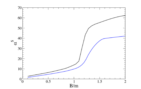
Figure 5: The coupling constant $\alpha=\lambda_{F}\lambda_{S}/(8\pi m)$, with $\lambda_{F(S)}$ the fermion (scalar) coupling in the interaction Lagrangian, vs the binding energy per unit mass. Blue solid line: exchanged mass, $\mu/m=0.15$. Black solid line: exchanged mass, $\mu/m=0.5$

.

6 Conclusions & Perspectives

The technique based on the Nakanishi integral representation of the BS amplitude has to be considered a viable and effective tool for solving BSE Indeed, the cross-check of results obtained by different groups, for different interacting systems, with kernels in ladder and cross-ladder contributions as well as with and without spin dofs, has produced a clear numerical evidence of the validity of NIR for obtaining actual solutions. Noteworthy, the possibility to obtain the valence component straightforwardly leads to evaluate relevant quantities, like the the LF momentum distributions, so important for phenomenological investigations.of bound systems in relativistic regime. In particular, one should remind the second ingredient of the technique, i.e. the LF framework. It has well-known advantages in performing analytical integrations, and in the fermionic case it shows its effectiveness in full glory.

The numerical validation of NIR strongly encourages to face with the next challenges represented by including self-energies and vertex corrections evaluated within the same framework (works in progress on the Dyson-Schwinger Equations) as well as by the possible construction of interaction kernels beyond the sum of the first two contributions in Fig. 2, e.g., moving from the fully off-shell ladder series, that fulfills an integral equation, to a closed form for the cross-ladder T-matrix.

References

- [1] Salpeter, E.E, Bethe, H.A, A Relativistic Equation for Bound-State Problems, Phys. Rev. 84, 1232 (1951). 10.1103/PhysRev.84.1232
- [2] Nakanishi, N, A General survey of the theory of the Bethe-Salpeter equation, Prog. Theor. Phys. Suppl. 43, 1 (1969). 10.1143/PTPS.43.1
- [3] Wick, G.C, Properties of Bethe-Salpeter Wave Functions, Phys. Rev. 96, 1124 (1954). 10.1103/PhysRev.96.1124
- [4] Zuilhof, M.J, Tjon, J.A, Electromagnetic Properties of the Deuteron and the Bethe-Salpeter Equation with One Boson Exchange, Phys. Rev. C 22, 2369 (1980). 10.1103/PhysRevC.22.2369
- [5] Lucha, W, Schoberl, F.F, Instantaneous Bethe-Salpeter equation with exact propagators, J. Phys. G 31, 1133 (2005). 10.1088/0954-3899/31/11/001
- [6] Gross, F, The CST: Its Achievements and Its Connection to the Light Cone, Few Body Syst. 58(2), 39 (2017). 10.1007/s00601-017-1215-4
- [7] Bondarenko, S.G, Burov, V.V, Molochkov, A.V, Smirnov, G.I, Toki, H, Bethe-Salpeter approach with the separable interaction for the deuteron, Prog. Part. Nucl. Phys. 48, 449 (2002). 10.1016/S0146-6410(02)00142-4
- [8] Cutkosky, R.E, Solutions of a Bethe-Salpeter equations, Phys. Rev. 96, 1135 (1954). 10.1103/PhysRev.96.1135
- [9] Nakanishi, N, Partial-Wave Bethe-Salpeter Equation, Phys. Rev. 130(3), 1230 (1963)
- [10] Kusaka, K, Simpson, K, Williams, A.G, Solving the Bethe-Salpeter equation for bound states of scalar theories in Minkowski space, Phys. Rev. D 56, 5071 (1997). 10.1103/PhysRevD.56.5071
- [11] Karmanov, V.A, Carbonell, J, Solving Bethe-Salpeter equation in Minkowski space, Eur. Phys. J.A 27, 1 (2006). 10.1140/epja/i2005-10193-0
- [12] Brodsky, S.J, Pauli, H.C, Pinsky, S.S, Quantum chromodynamics and other field theories on the light cone, Phys. Rept. 301, 299 (1998). 10.1016/S0370-1573(97)00089-6
- [13] Carbonell, J, Desplanques, B, Karmanov, V.A, Mathiot, J.F, Explicitly covariant light front dynamics and relativistic few body systems, Phys. Rept. 300, 215 (1998). 10.1016/S0370-1573(97)00090-2
- [14] Carbonell, J, Karmanov, V.A, Cross-ladder effects in Bethe-Salpeter and light-front equations, Eur. Phys. J. A 27, 11 (2006). 10.1140/epja/i2005-10194-y
- [15] de Paula, W, Frederico, T, Salmè, G, Viviani, M, Advances in solving the two-fermion homogeneous Bethe-Salpeter equation in Minkowski space, Phys. Rev. D 94, 071901 (2016). 10.1103/PhysRevD.94.071901
- [16] de Paula, W, Frederico, T, Salmè, G, Viviani, M, Pimentel, R, Fermionic bound states in Minkowski-space: Light-cone singularities and structure, Eur. Phys. J. C77(11), 764 (2017). 10.1140/epjc/s10052-017-5351-2
- [17] Lurié, D, Macfarlane, A.J, Takahashi, Y, Normalization of Bethe-Salpeter Wave Functions, Phys. Rev. 40, B1091 (1965). 10.1103/PhysRev.140.B1091
- [18] Nakanishi, N, Normalization Condition and Normal and Abnormal Solutions of the Bethe-Salpeter Equation, Phys. Rev. 138, B1182 (1965). 10.1103/PhysRev.138.B1182
- [19] Ahlig, S, Alkofer, R, (In)consistencies in the relativistic description of excited states in the Bethe-Salpeter equation, Annals Phys. 275, 113 (1999). 10.1006/aphy.1999.5922
- [20] Nakanishi, N, Graph Theory and Feynman Integrals (Gordon and Breach, New York, 1971)
- [21] Frederico, T, Salmè, G, Viviani, M, Quantitative studies of the homogeneous Bethe-Salpeter equation in Minkowski space, Phys. Rev. D 89, 016010 (2014). 10.1103/PhysRevD.89.016010
- [22] Frederico, T, Salmè, G, Viviani, M, Two-body scattering states in Minkowski space and the Nakanishi integral representation onto the null plane, Phys. Rev. D 85, 036009 (2012). 10.1103/PhysRevD.85.036009
- [23] Carbonell, J, Karmanov, V.A, Solving Bethe-Salpeter equation for two fermions in Minkowski space, Eur. Phys. J. A 46, 387 (2010). 10.1140/epja/i2010-11055-4
- [24] Yan, T.M, Quantum Field Theories in the Infinite-Momentum Frame. IV. Scattering Matrix of Vector and Dirac Fields and Perturbation Theory, Phys. Rev. D 7, 1780 (1973). 10.1103/PhysRevD.7.1780
- [25] Nogueira, J.H.A, et al, To be published (2019)
- [26] Gutierrez, C, Gigante, V, Frederico, T, Salmè, G, Viviani, M, Tomio, L, Bethe-Salpeter bound-state structure in Minkowski space, Phys. Lett. B 759, 131 (2016). 10.1016/j.physletb.2016.05.066
- [27] Frederico, T, Salmè, G, Viviani, M, Solving the inhomogeneous Bethe–Salpeter equation in Minkowski space: the zero-energy limit, Eur. Phys. Jou. C 75(8), 398 (2015). 10.1140/epjc/s10052-015-3616-1
- [28] Gigante, V, Nogueira, J.H.A, Ydrefors, E, Gutierrez, C, Karmanov, V.A, Frederico, T, Bound state structure and electromagnetic form factor beyond the ladder approximation, Phys. Rev. D 95(5), 056012 (2017). 10.1103/PhysRevD.95.056012