Analysis of the interaction between classical and quantum plasmons via FDTD-TDDFT method

Abstract

A powerful hybrid FDTD–TDDFT method is used to study the interaction between classical plasmons of a gold bowtie nanoantenna and quantum plasmons of graphene nanoflakes (GNFs) placed in the narrow gap of the nanoantenna. Due to the hot-spot plasmon of the bowtie nanoantenna, the local-field intensity in the gap increases significantly, so that the optical response of the GNF is dramatically enhanced. To study this interaction between classical and quantum plasmons, we decompose this multiscale and multiphysics system into two computational regions, a classical and a quantum one. In the quantum region, the quantum plasmons of the GNF are studied using the TDDFT method, whereas the FDTD method is used to investigate the classical plasmons of the bowtie nanoantenna. Our analysis shows that in this hybrid system the quantum plasmon response of a molecular-scale GNF can be enhanced by more than two orders of magnitude, when the frequencies of the quantum and classical plasmons are the same. This finding can be particularly useful for applications to molecular sensors and quantum optics.

I Introduction

The interaction of light with metallic nanoparticles has been a central theme in plasmonics [1, 2, 3] ever since the beginnings of this discipline. In particular, electromagnetic waves can induce collective oscillations of free electrons in metals, giving rise to so-called plasmon modes. In recent years, plasmons in two-dimensional (2D) materials, such as graphene, have attracted increasing research interest, primarily because of the new rich physics characterizing these materials. For instance, since plasmons are confined in a very small region, the induced optical near-field in these low-dimensional materials can be enhanced and localized in extreme-subwavelength regions [3, 4], which can be used, e. g. to plasmon-enhanced spectroscopy [5] and light concentration beyond diffraction limit [6, 7]. Moreover, these properties are dependent on the material structure and geometrical configuration of the plasmonic system, its size, and the electromagnetic properties of the surrounding medium [8, 9], thus they can be readily tuned. As a result, plasmonic effects have found a plethora of applications, including the design of highly integrated nanophotonic systems [4, 6, 10, 11], nanophotonic lasers and amplifiers [7, 12], new optical metamaterials [13], nanoantennas [5, 14], single-molecule spectroscopy [15], photovoltaic devices [16, 17], surface-enhanced Raman scattering [5, 18], higher-harmonic light generation [19, 20, 21, 22], catalytic monitoring of reactant adsorption [23], sensing of electron charge-transfer events [24], and biosensing [25, 26].

When the geometrical size of plasmonic nanoparticles is less than about $10\text{\,}\mathrm{nm}$, the description of their optical properties becomes more challenging because quantum effects begin to play an important role. At this scale, plasmon resonances become more sensitive to the quantum nature of the conduction electrons [9], thus the theoretical predictions of approaches based entirely on the Maxwell equations are less successful in describing experimental results [27, 28]. The shortcomings of the classical theory stem chiefly from neglecting three quantum effects: i) spill-out of electrons at medium boundaries [29, 30], ii) surface-enabled electron-hole pair creation [31, 32, 33], and iii) nonlocal effects of electron wavefunction [34, 35]. These quantum effects can significantly change the features of plasmon spectra predicted by the classical theory [36, 37, 38]. For example, the spill-out effect results in an inhomogeneous permittivity around the nanoparticle boundary, a phenomenon responsible for the size-dependent frequency shift of plasmon resonances [3, 9, 28, 39]. In order to overcome these shortcomings of the classical theory, a new research area that combines plasmonics with quantum mechanics, known as quantum plasmonics, has recently emerged [3, 7, 29, 39].

Theoretical and experimental advances in plasmonics have been greatly facilitated by the development of efficient numerical methods. In the classical regime, the physical properties of plasmonic nanostructures can be modeled numerically by solving the Maxwell equations using specific computational electromagnetic methods, such as the finite-difference time-domain (FDTD) method [40]. In these computational methods, the classical plasmon features are mainly derived from the specific geometrical configuration of the plasmonic system and the distribution of the (local) dielectric function. As long as the size of a plasmonic system is large enough, its electromagnetic response is very well described by this computational classical approach. However, if the size of nanoparticles is smaller than about $10\text{\,}\mathrm{nm}$, quantum effects must be included in the computational description of plasmonic nanostructures. One such numerical method, widely used in quantum plasmonics, is the time-dependent density functional theory (TDDFT) [41, 42]. In particular, it has been used to describe the dynamic response of plasmonic systems and the corresponding optical spectra [37, 43]. However, TDDFT calculations are very time and memory consuming, thus most TDDFT simulations are limited to small nanoparticles (generally, less than a few hundreds atoms) [44, 45].

Driven by the need to describe the physical regime in which classical and quantum effects play comparable roles, there has recently been growing interest in developing classical-quantum hybrid methods that can address this regime. For example, several numerical methods that aim to describe strongly-coupled classical-quantum hybrid systems were proposed [46, 47, 48, 49, 50] and used to investigate phenomena such as super-radiance, Rabi splitting, and nonlinear harmonic generation. However, in order to optimize the computational costs and simplify the numerical analysis, some recent works [51, 52, 53] demonstrated that in specific situations it is enough to only consider the direct coupling of the classical system to the quantum one and neglect the back coupling (the so-called weak-coupling regime). Here, we should note such decoupled analysis assumption is only applicable in the weak-coupling regime. In the strong-coupling regime, full-quantum methods or two-way-coupling classical-quantum simulations should be used.

One such physical system is studied in our paper, namely we apply an FDTD–TDDFT hybrid numerical method [51] to study the classical-quantum plasmon interaction in the weak-coupling regime. In particular, we investigate the interaction between a classical plasmon of a bowtie nanoantenna and a quantum plasmon of a graphene nanoflake (GNF) in the weak-coupling limit. In this multiphysics and multiscale approach, the classical optical response of the bowtie nanoantenna is computed using the FDTD method, whereas the quantum optical properties of the molecular-scale GNF are determined using the TDDFT. Importantly, we employ the local field calculated with the FDTD method as excitation field used in the quantum mechanical calculations, thus bridging the descriptions of the classical and quantum components of the hybrid plasmonic nanosystem.

The remainder of this paper is organized as follows. In Sec. II, we present the multiphysical system investigated in this study, and the corresponding computational methods are presented as well. In Sec. III, we first describe the optical properties of the plasmons of the GNF and bowtie nanoantenna, respectively, and then the main features of the interaction between these two types of plasmons is presented. Finally, the main conclusions are summarized in the last section.

II Multiphysical system and computational methods

The physical system used to illustrate the main features of our numerical method is shown in Fig. 1. It consists of a gold bowtie nanoantenna placed on a silica substrate and a molecular-scale GNF located in the narrow gap of the nanoantenna. The nanoantenna is made of two triangular gold plates with angle, $\alpha$, length, $L$, and thickness, $t$, the separation distance between the tips of the gold plates being $\Delta$. By properly choosing the computational grid, we made sure that the edges of the two triangular gold plates were flat. In all our simulations $\alpha=$$$, $\Delta=$10\text{\,}\mathrm{nm}$$, and $t=$30\text{\,}\mathrm{nm}$$, but $L$ will be varied. Moreover, we assume that the GNF has a triangular shape, too, with side length, $a=$1.23\text{\,}\mathrm{nm}$$, namely there are six carbon atoms along each side of the triangle. It should be noted that triangular GNFs is one of the stable configurations in which they exist [54]. The GNF is positioned in such a way that its symmetry axis coincides with the longitudinal axis of the nanoantenna.

The bowtie nanoantenna has plasmon resonances associated with the triangular plates and strongly localized (hot-spot) plasmons generated in the narrow gap of the nanoantenna. Given the size of the bowtie nanoantenna, the spectral characteristics of these plasmons can be determined by solving the Maxwell equations. The physics of the molecular-scale GNF, on the other hand, must be described using quantum mechanics based numerical methods. Due to the large size difference between the two plasmonics systems, there is a very large mismatch between the computational grids on which the classical and quantum dynamics are resolved, as well as the corresponding time scales. Before we describe the hybrid numerical method that allows one to overcome these difficulties, we will briefly present the FDTD and TDDFT methods used in the classical and quantum computations, respectively.

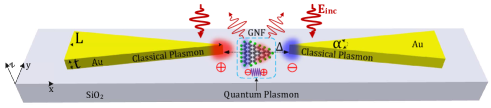
Figure 1: Multiphysical system of a classical and quantum hybrid plasmon model, where the quantum plasmon of a graphene nanoflake interacts with the classical plasmon of a gold bowtie nanoantenna via the optical near-field.

In order to numerically solve Maxwell’s equations using the FDTD method [40], one should discretize them on the Yee grid. As a result of this procedure, one obtains the following system of iterative equations:

$$\left.{{E_{d}}}\right|_{i,j,k}^{n+1}={\alpha_{1}}\left.{{E_{d}}}\right|_{i,j,k}^{n}+{\alpha_{2}}\left({\left.{\Delta{l_{d-1}}{{\bar{H}}_{d-1}}}\right|_{i,j,k}^{n+\frac{1}{2}}}\right.$$ (1)

$$\left.{-\left.{\Delta{l_{d+1}}{{\bar{H}}_{d+1}}}\right|_{i,j,k}^{n+\frac{1}{2}}-\left.{\Delta s_{d}{J_{s,d}}}\right|_{i,j,k}^{n+\frac{1}{2}}}\right)$$

$$\left.{{H_{d}}}\right|_{i,j,k}^{n+\frac{1}{2}}={\beta_{1}}\left.{{H_{d}}}\right|_{i,j,k}^{n-\frac{1}{2}}+{\beta_{2}}\left({\left.{\Delta{l_{d+1}}{{\bar{E}}_{d+1}}}\right|_{i,j,k}^{n}}\right.$$ (2)

$$\left.{-\left.{\Delta{l_{d-1}}{{\bar{E}}_{d-1}}}\right|_{i,j,k}^{n}-\left.{\Delta s_{d}{M_{s,d}}}\right|_{i,j,k}^{n}}\right)$$

Here, the subscripts $i$, $j$, and $k$ indicate the grid points on the Yee grid, and $d=x$, $y$, and $z$ indicates the field component. The subscript $d$ is used in a circular way, i.e. if $d=x$, then $d-1=z$ and $d+1=y$. The area of each face of the Yee grid is calculated as $\Delta s_{d}=\Delta l_{d-1}\Delta l_{d+1}$, where $\Delta l_{d}$ is the length of the corresponding edge. Moreover, the time step is indicated by an integer $n$, and the spatial difference operator is represented by $\bar{E}$ and $\bar{H}$, which are defined as follows:

$$\left.{{{\bar{E}}_{d\pm 1}}}\right|_{i,j,k}^{n}=\left.{{E_{d\pm 1}}}\right|_{{{\left\langle{i,j,k}\right\rangle}_{d\mp 1}}+1}^{n}-\left.{{E_{d\pm 1}}}\right|_{i,j,k}^{n}$$ (3)

$$\left.{{{\bar{H}}_{d\pm 1}}}\right|_{i,j,k}^{n}=\left.{{H_{d\pm 1}}}\right|_{{{\left\langle{i,j,k}\right\rangle}_{d\mp 1}}+1}^{n}-\left.{{H_{d\pm 1}}}\right|_{i,j,k}^{n}$$ (4)

Here, the notation $<i,j,k>_{d\pm 1}+1$ indicates a shift of the grid index ($i$,$j$,$k$) with respect to the subscript $d\pm 1$. For instance, when $d=x$, we have $d-1=z$, thus the notation $<i,j,k>_{d-1}+1=<i,j,k>_{z}+1=(i,j,k+1)$. Moreover, the iteration coefficients in Eqs. (1) and (2) are

$${\alpha_{1}}=(2\varepsilon-\sigma_{e}\Delta t)/(2\varepsilon+\sigma_{e}\Delta t)$$ (5)

$${\alpha_{2}}={2\Delta t}/{\left[({2\varepsilon+\sigma_{e}\Delta t})\Delta s\right]}$$ (6)

$${\beta_{1}}=(2\mu-\sigma_{m}\Delta t)/(2\mu+\sigma_{m}\Delta t)$$ (7)

$${\beta_{2}}={2\Delta t}/{\left[({2\mu+\sigma_{m}\Delta t})\Delta s\right]}$$ (8)

where $\Delta t$ is the time step, $\varepsilon$ is the electric permittivity, $\mu$ is the magnetic permeability, $\sigma_{e}$ is the electric conductivity, $\sigma_{m}$ is the equivalent magnetic loss.

Based on the formalism described above, an FDTD iteration is performed by repeating the following three steps until a preset convergence criterion is satisfied [55]: In Step 1, using the spatial distribution of the fields $H$ and $E$ at the time steps $n-\frac{1}{2}$ and $n$, respectively, one updates the $H$ field at the time step $n+\frac{1}{2}$ via Eq. (2). In Step 2, using the spatial distribution of the fields $H$ and $E$ at the time steps $n+\frac{1}{2}$ and $n$, respectively, one updates the $E$ field at the time step $n+1$ via Eq. (1). Finally, at Step 3, one sets $n=n+1$ in Step 1 and repeats Step 1 through Step 3. At the end of each iteration one verifies whether the preset convergence criterion is satisfied.

The quantum mechanical calculations are based on the TDDFT method, which we briefly present in what follows. One starts from the Schrödinger equation,

$$i\hbar\frac{\partial}{\partial t}\ket{\Psi(t)}=\hat{H}\ket{\Psi(t)},$$ (9)

where $\hat{H}$ is the Hamiltonian of the system, $\ket{\Psi(t)}$ is the many-body wavefunction, and $\hbar$ is the reduced Planck constant. In the general case, the Hamiltonian of the system can be written as:

$$\hat{H}={\hat{T}_{n}}+{\hat{T}_{e}}+{\hat{V}_{nn}}+{\hat{V}_{ee}}+{\hat{V}_{ne}}+{\hat{V}_{s}},$$ (10)

where $\hat{T}_{n}$ and $\hat{T}_{e}$ are the kinetic energy of the nuclei and electrons, respectively, $\hat{V}_{nn}$ and $\hat{V}_{ee}$ are the nuclei-nuclei and electron-electron Coulomb interactions, respectively, $\hat{V}_{ne}$ is the nuclei-electron potential, and $\hat{V}_{s}$ is the external potential, e.g. the interaction potential with an applied external electric field (for more details, see [41, 42]).

For a general many-body system, the complexity of Eq. (9) makes it very challenging to solve it directly, especially for systems with large number of electrons. In order to overcome this challenge, one usually employs two approximations: i) One assumes that the properties of atoms are mainly determined by the valence electrons, and ii) the ionic cores are assumed to be fixed. Moreover, using the Hohenberg-Kohn [56] and Runge-Grosss [57] theorems, the many-body wavefunction is expressed as a Slater determinant formed with single-particle orbitals of a noninteracting system, $\psi_{i}(\mathbf{r},t)$, whose dynamics are determined by the effective Kohn-Sham Hamiltonian, $\hat{H}_{KS}$:

$$i\hbar\frac{\partial}{\partial t}\psi_{i}(\mathbf{r},t)=\hat{H}_{KS}(\mathbf{r},t)\psi_{i}(\mathbf{r},t).$$ (11)

In this formalism, the effective Kohn-Sham Hamiltonian is expressed as follows:

$$\hat{H}_{KS}(\mathbf{r},t)= \hat{T}_{e}(\mathbf{r},t)+\hat{V}_{H}[\rho(\mathbf{r},t)]+\hat{V}_{xc}[\rho(\mathbf{r},t)]$$

$$+\hat{V}_{ne}(\mathbf{r},t)+\hat{V}_{s}(\mathbf{r},t),$$ (12)

where the Hartree potential, $\hat{V}_{H}[\rho(\mathbf{r},t)]$, which represents the classical Coulomb electron-electron interaction and the exchange-correlation potential, $\hat{V}_{xc}[\rho(\mathbf{r},t)]$, are functionals that depend on the electron charge density,

$$\rho(\mathbf{r},t)=\sum_{i}|\psi_{i}(\mathbf{r},t)|^{2}$$ (13)

It should be noted that the exchange-correlation potential ${V_{xc}}[{\rho({{\bf{r}},t})}]$ is generally unknown, so that in practice several approximations of various degrees of sophistication are used, including the local density approximation [58] and the generalized gradient approximation [59].

In summary, a self-consistent TDDFT iteration consists of four steps. Step 1: The ground-state wavefunction is calculated using the DFT method and then is used to construct the initial electron density, $\rho(\mathbf{r},t_{k})$. Step 2: The Hamiltonian $\hat{H}_{KS}$ defined by Eq. (II), corresponding to the time step $t_{k}$, is constructed using the electron density $\rho(\mathbf{r},t_{k})$. Step 3: Using the Hamiltonian $\hat{H}_{KS}$ and Kohn-Sham orbitals $\psi_{i}$ calculated at $t_{k}$, the orbitals $\psi_{i}$ and the electron charge density $\rho(\mathbf{r},t_{k+1})$ at the time step $t_{k+1}$ are calculated using a proper time propagator [60]. Step 4: test the convergence criterion. If convergence is reached, the iteration is stopped, otherwise the iteration is repeated from Step 2.

The two computational methods, FDTD and TDDFT, are decoupled and can be used independently of each other. There is, however, a way to use them together when one aims to describe physical systems that contain both classical and quantum components. We illustrate this approach on our plasmonic system. Thus, we use first an FDTD simulation to determine the optical spectrum of the gold bowtie nanoantenna and the time dependence of the electric field at the location of the GNF. Then, in a subsequent simulation, this electric field is used as excitation field (external potential) in an TDDFT simulation and the corresponding optical spectra of the GNF are computed. This hybrid computational approach rigourously takes into account the influence of the classical plasmon of the bowtie nanoantenna on the quantum plasmon of the GNF and the accompanying field enhancement effects, but it does not incorporate the back-coupling effect of the quantum plasmon on the classical one. It is expected that this effect is very small considering the size mismatch between the classical and quantum objects, which would mean that our method provides reliable predictions.

In order to validate this key assumption, we have calculated the absorption spectra of an isolated gold bowtie nanoantenna, an isolated GNF, and a bowtie-GNF classical system, with the results of this analysis being presented in Fig. 2. In these calculations, the length of bowtie antenna was $L=$280\text{\,}\mathrm{nm}$$ and the side length of triangular GNF was $1\text{\,}\mathrm{nm}$, whereas the dielectric constant of the GNF was described by a model presented in [61]. In order to make the GNF system share the same resonance frequency as the bowtie antenna system. The Fermi energy of graphene is chosen as $0.52\text{\,}\mathrm{eV}$, relaxation time of $0.1\text{\,}\mathrm{ps}$, and temperature of $300\text{\,}\mathrm{K}$. Fig. 2(a) show the absorption of an isolated GNF, an isolated bowtie antenna, and the GNF and bowtie in the bowtie-GNF hybrid system. Moreover, the corresponding field distributions of these systems at the resonance frequency in Fig. 2(a) are given in Figs. 2(c)-2(d).

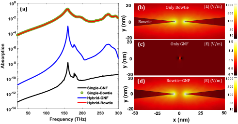
Figure 2: Classical simulation. (a) Absorption of an isolated GNF, an isolated bowtie antenna, GNF in a bowtie-GNF hybrid system, and bowtie in a bowtie-GNF hybrid system. The absorption in the bowtie nanoantenna corresponds to the domains shown in the right panels and not the entire nanoantenna. (b), (c), (d) Field-distributions of an isolated bowtie nanoantenna, an isolated GNF, and a bowtie-GNF hybrid system, respectively.

These results clearly validate our premise, namely that the influence of the GNF on the bowtie nanoantenna is negligible. Thus, Fig. 2(a) shows that there is practically a complete overlap between the absorption spectrum of the isolated bowtie and that of the bowtie in the bowtie-GNF hybrid system, which proves that the presence of the GNF does not affect the bowtie nanoantenna. Moreover, the field profiles show that, at resonance, the electric field created inside the bowtie nanoantenna gap is up to $1000\times$ larger than the field around an isolated GNF. In addition, the field profiles in Figs. 2(b) and 2(d) suggest that the fields in the isolated bowtie nanoantenna and the bowtie-GNF hybrid system are practically identical. This demonstrates that the scattering field of the GNF is negligible as compared to the field in the bowtie-GNF system.

III Results and Discussion

III-A Quantum plasmons of graphene nanoflakes

We considered first the GNFs described in the preceding section and used the TDDFT method to investigate their optical spectra. More specifically, we used the Octopus-TDDFT code package [62], and employed the generalized gradient approximation with the Perdew-Burke-Ernzerhof parametrization [63]. The GNF is freestanding and it only interacts with an external time-dependent and spatially constant electric field. We assumed that the time dependence of the field was described by a delta-function and it was $x$-polarized. We have performed these calculations for an undoped GNF and for GNFs with charge doping concentrations of $7\text{\,}\mathrm{\char 37\relax}$ and $15\text{\,}\mathrm{\char 37\relax}$. Here, the charge doping concentration is defined as the ratio of the number of excess charges to the number of carbon atoms in the GNF. The computations were performed on a computer platform containing Intel^® Xeon^® E5-2640v3 CPUs and 4 cores (4 GB RAM per core) were used in a generic simulation. Each TDDFT simulation required 1.04 GB of memory and was performed in about 50 hours.

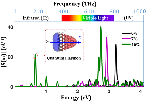
Figure 3: Quantum simulation: Absorption spectra of a graphene nanoflake calculated for several values of the charge doping concentration. In inset, the charge distribution determined at the plasmon resonance frequency.

The quantum response of the GNF is quantified by the dipole strength function,

$$S_{ij}(\omega)=2\omega\verb"Im"[\alpha_{ij}(\omega)]/\pi$$ (14)

where the polarizability $\alpha_{ij}(\omega)$ is defined as:

$$\alpha_{ij}(\omega)=\frac{1}{|E_{j}|}\int[p_{i}(t)-p_{i}(0)]e^{-i\omega t}dt,$$ (15)

where $i,j=x,y,z$ and $|E_{j}|$ is the amplitude of the $j$th component of the external electric field. Moreover, the dynamical dipole moment $p_{i}(t)$ is evaluated as:

$$p_{i}(t)=\int\rho(\mathbf{r},t)r_{i}d\mathbf{r}.$$ (16)

This approach has been used to calculate the absorption spectrum of the triangular GNF, the corresponding results being presented in Fig. 3. It can be seen in this figure that the main resonance peak of the undoped GNF is located in the ultraviolet region, whereas when the charge doping concentration is increased to $15\text{\,}\mathrm{\char 37\relax}$ another resonance peak is formed in the infra-red region. Moreover, the spectra presented in Fig. 3 show that the plasmon frequency decreases as the charge doping concentration increases, whereas the amplitude of the peaks increases with the increase of the doping concentration. More importantly, new resonance peaks emerge when the charge doping concentration increases. In order to gain more physical insights into the nature of these resonances, we have calculated the distribution of the net charge density at the resonance frequencies, as compared to that in the ground state. In the inset of Fig. 3, we plot the corresponding results, determined for the GNF with $15\text{\,}\mathrm{\char 37\relax}$ doping concentration. The blue and red colors correspond to the negative and positive net charge density, respectively. This net charge distribution does prove that this resonance peak corresponds to collective electron density oscillations, i.e. it can be viewed as a quantum plasmon.

III-B Classical plasmons of gold bowtie

The second part of our study consists of the calculation of the optical spectra of the gold bowtie nanoantenna, which is schematically illustrated in Fig. 4(a). The nanoantenna is illuminated by a normally incident plane wave with the frequency ranging from $50\text{\,}\mathrm{THz}300\text{\,}\mathrm{THz}$ and the electric field is polarized along the $x$-axis. In order to determine the optical spectrum of the nanoantenna, we computed the electric field at certain locations in the gap using the FDTD method and then Fourier transformed it to the frequency domain. The computations were performed on a desktop computer with a quad-core Intel^® Core^™ i7-4790 CPU with 8 GB RAM per core. One such simulation required about 110 MB of memory and was performed in about 42 minutes.

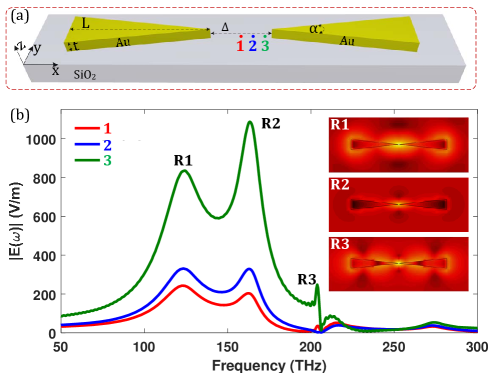
Figure 4: (a) Configuration of a gold bowtie nanoantenna and the locations where the optical near-field is probed. (b) The optical spectra corresponding to the locations indicated in panel (a). The insets show the profiles of the amplitude of the electric field, calculated at the resonances $R_{1}$, $R_{2}$, and $R_{3}$.

The results of these calculations, determined for a nanoantenna with $L=$500\text{\,}\mathrm{nm}$$, are summarized in Fig. 4(b). For a better comparison among the spectra, we have normalized the spectra $|E(\omega)|$ to the amplitude of the incident electric field. The spectra presented in Fig. 4(b) reveal several important features. First, all spectra possess a series of resonances, the corresponding resonance frequencies being the same for all spectra. Second, the amplitude of the optical near-field is enhanced by more than two orders of magnitude at some particular resonance frequencies, with the enhancement factor varying with the probing point.

In order to gain more physical insights into the characteristics of these resonances, we have calculated the electric field profiles corresponding to the frequencies of the main spectral peaks. The resulting plots, shown as insets in Fig. 4(b), reveal several important findings: the resonance marked with $R_{1}$ represents the fundamental plasmon of the entire bowtie nanoantenna, the resonance $R_{2}$ corresponds to a strongly localized plasmon formed in the narrow gap of the nanoantenna (a so-called hot-spot plasmon), and the resonance $R_{3}$ represents the second-order plasmon of the bowtie nanoantenna. Note that the resonance wavelength of the hot-spot plasmon depends only on the shape of the plasmonic cavity and dielectric environment of the plasmonic cavity. Moreover, particularly relevant to our study is the fact that the hot-spot plasmon is strongly confined in the gap of the bowtie nanoantenna, which would lead to a strong field overlap and implicitly enhanced interaction with the quantum plasmon of a GNF placed in the gap.

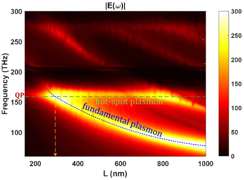
Figure 5: Dispersion map of the field enhancement spectra of the gold bowtie nanoantenna, calculated at the probe position “1” shown in Fig. 4(a).

An enhanced interaction between the quantum plasmon of the GNF and the hot-spot plasmon of the bowtie nanoantenna is achieved if these two plasmons have the same frequency. Therefore, in order to reach this strongly enhanced interaction regime, we optimized the geometric structure of the nanoantenna by varying the length $L$ so that the frequencies of these two resonances coincide. More specifically, we scanned $L$ from $100\text{\,}\mathrm{nm}1000\text{\,}\mathrm{nm}$ while keeping constant the values of all the other simulation parameters. The dispersion map of the corresponding field enhancement spectra, calculated at the probe position ”1” in Fig. 4(a), is given in Fig. 5.

The dispersion map of the field enhancement possesses a series of bands, which correspond to different plasmons of the system. Of all these bands, two are particularly important for our study. The first is the plasmon band whose corresponding plasmon frequency does not depend on $L$. This band corresponds to the hot-spot plasmon as the frequency of this plasmon depends only on the electromagnetic environment around the narrow gap of the bowtie nanoantenna. Moreover, there is a second plasmon band whose plasmon frequency varies with $L$. This band corresponds to the fundamental plasmon of the nanoantenna. Moreover, the hot-spot plasmon band and the fundamental plasmon band cross at $L=$280\text{\,}\mathrm{nm}$$, the corresponding frequency being $159\text{\,}\mathrm{THz}$. Importantly, this frequency is equal to the frequency of the quantum plasmon of the GNF with $15\text{\,}\mathrm{\char 37\relax}$ doping concentration. This means that for $L=$280\text{\,}\mathrm{nm}$$ the quantum plasmon of the GNF, the hot-spot plasmon, and the fundamental plasmon of the nanoantenna have practically the same frequency. We expect, therefore, to observe an enhanced interaction among these plasmons for this configuration of the hybrid plasmonic system.

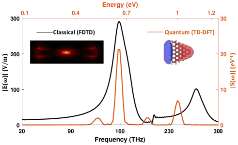
Figure 6: Spectra of the bowtie nanoantenna with $L=$280\text{\,}\mathrm{nm}$$ (black line) and GNF with a doping concentration of $15\text{\,}\mathrm{\char 37\relax}$ (red line). In insets, the profile of the optical near-field of the hot-spot plasmon and the charge distribution of the quantum plasmon, calculated at the resonance frequency.

III-C Interaction between classical and quantum plasmons

The interaction between the classical and quantum plasmons can be characterized quantitatively by analyzing the combined hybrid plasmonic system. In order to illustrate the fact that the two types of plasmons have the same frequency when $L=$280\text{\,}\mathrm{nm}$$, we present in Fig. 6 the corresponding spectrum of the bowtie nanoantenna and the spectrum of the GNF corresponding to a doping concentration of $15\text{\,}\mathrm{\char 37\relax}$. These spectra clearly show that the two plasmon resonances are located at the same frequency of $159\text{\,}\mathrm{THz}$. In addition, the profile of the optical near-field of the hot-spot plasmon and the charge distribution of the quantum plasmon, calculated at the resonance frequency, further support the plasmonic nature of these resonances. Importantly, the spectrum of the bowtie nanoantenna suggests that at the resonance frequency the field amplitude in the gap of the nanoantenna can be enhanced by more than two orders of magnitude.

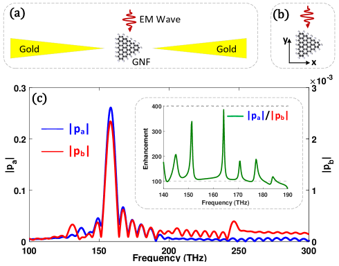
Figure 7: (a), (b) Schematics of a GNF placed in the gap of a gold bowtie nanoantenna and of an isolated GNF, respectively. (c) Spectra of the dipole moments $|p_{a}|$ and $|p_{b}|$ corresponding to the configurations shown in panels Fig.6(a) and 6(b), respectively, and calculated under the same plane wave excitation conditions. In inset, the spectrum on the enhancement of the quantum plasmon response defined as the ratio $|p_{a}|/|p_{b}|$.

In order to assess the influence of this remarkable field enhancement effect induced by the hot-spot plasmon resonance of bowtie nanoantenna on the quantum plasmon of the GNF, we place such a GNF at the center of the gap of the optimized bowtie nanoantenna, as illustrated in Fig. 7(a). Then, using the hybrid FDTD–TDDFT method, we determined the spectrum of the GNF. As discussed, this is performed in two steps. First, we run an FDTD computation to determine the time-dependent electric field at the location of the GNF under a pulsed plane wave excitation whose frequency ranges from $100\text{\,}\mathrm{THz}300\text{\,}\mathrm{THz}$. Then, in the second step, we used this field as external excitation of the GNF in an TDDFT simulation. For reference, we also calculated the spectrum of the GNF without the nanoantenna but under the same pulsed plane wave excitation conditions, as depicted in Fig. 7(b). The computations were performed on a computer platform containing Intel^® Xeon^® E5-2640v3 CPUs and 4 cores (4 GB RAM per core) were used in a generic simulation. One such FDTD–TDDFT simulation of the classical-quantum hybrid system shown in Fig. 7(a) required about 1.16 GB of memory and wall-clock time of 23.5 days, whereas a TDDFT simulation of the quantum system presented in Fig. 7(b) required 1.04 GB of memory and 6.8 days wall-clock time.

The results of this computational analysis are summarized in Fig. 7. In Figs. 7(a) and 7(b), we present the two system configurations, whereas in Fig. 7(c) we show the spectra of the amplitude of the dipole moments, $|p_{a}|$ and $|p_{b}|$, corresponding to the two systems. For a better comparison, we plot in the inset of Fig. 7(c) the ratio $|p_{a}|/|p_{b}|$, which can be viewed as the parameter that best quantifies the enhancement of the quantum plasmon excitation. The two spectra suggest that the frequency of the quantum plasmon of the GNF is not affected by the excitation of the hot-spot plasmon, which means that, as expected, the effects of the quantum plasmon on the classical one are negligible. More importantly, however, it can be seen that the response of the quantum plasmon of the GNF can be enhanced by more than two orders of magnitude upon interaction with the hot-spot plasmon of a specially designed gold bowtie nanoantenna.

IV Conclusions

In summary, we have applied a hybrid FDTD–TDDFT approach to study the interaction between classical and quantum plasmons of a multiscale and multiphysical system, where a molecular-scale graphene nanoflake is placed in the gap of a gold bowtie nanoantenna. The TDDFT simulation of the graphene nanoflake shows that it possesses a quantum plasmon in the infrared regime if the graphene is doped with some excess charges. We also demonstrated that the excitation of this quantum plasmon can be significantly enhanced if the graphene nanoflake is placed inside the narrow gap of a specially designed gold bowtie nanoantenna that possesses a hot-spot gap plasmon resonance at the same frequency as that of the quantum plasmon of the graphene nanoflake. In particular, by combining FDTD simulations of the bowtie nanoantenna and TDDFT calculations of the optical response of the graphene nanoflake, we show that in the presence of the bowtie nanoantenna the quantum plasmon response of the graphene nanoflake can be enhanced by more than two orders of magnitude.

References

- [1] S. A. Maier, Plasmonics: Fundamentals and Applications, Springer, 2007.
- [2] M. Pelton and G. W. Bryant, Introduction to Metal-Nanoparticle Plasmonics, John Wiley, 2013.
- [3] A. Varas, P. Garcia-Gonzalez, J. Feist, F.J. Garcia-Vidal, and A. Rubio, “Quantum plasmonics: from jellium models to ab initio calculations,” Nanophotonics, vol. 5, no.3, pp.409-426, 2016.
- [4] J. A. Schuller, E. S. Barnard, W. Cai, Y. C. Jun, J. S. White, and M. L. Brongersma, “Plasmonics for extreme light concentration and manipulation,” Nat. Mater., vol.9, no.3, pp.193, 2010.
- [5] H. Xu, E. J. Bjerneld, M. Kall, and L. Borjesson, “Spectroscopy of single hemoglobin molecules by surface enhanced Raman scattering,” Phys. Rev. Lett., vol.83, no.21, pp.4357, 1999.
- [6] D. K. Gramotnev, and S. I. Bozhevolnyi, “Plasmonics beyond the diffraction limit,” Nat. Photonics, vol.4, no.2, pp.83, 2010.
- [7] M. S. Tame, K. R. McEnery, S. K. Ozdemir, J. Lee, S. A. Maier, and M. S. Kim, “Quantum plasmonics,” Nat. Phys., vol.9, no.6, pp.329, 2013.
- [8] K. A. Willets, and R. P. Van Duyne, 2007. “Localized surface plasmon resonance spectroscopy and sensing,” Annu. Rev. Phys. Chem., vol.58, pp.267-297, 2007.
- [9] J. A. Scholl, A. L. Koh, and J. A. Dionne, “Quantum plasmon resonances of individual metallic nanoparticles,” Nature, vol.483, no.7390, pp.421, 2012.
- [10] N. C. Panoiu and R. M. Osgood, “Subwavelength Nonlinear Plasmonic Nanowire,” Nano Lett., vol.4, pp.2427-2430, 2004.
- [11] M. I. Stockman, “Nanofocusing of optical energy in tapered plasmonic waveguides,” Phys. Rev. Lett., vol.93, pp.137404, 2004.
- [12] P. Berini, and I. De Leon, “Surface plasmon-polariton amplifiers and lasers,” Nat. Photonics, vol.6, no.1, pp.16, 2012.
- [13] O. Hess, J. B. Pendry, S. A. Maier, R. F. Oulton, J. M. Hamm, and K. L. Tsakmakidis, “Active nanoplasmonic metamaterials,” Nat. Mater., vol.11, no.7, pp.573, 2012.
- [14] V. Giannini, A. I. Fernandez-Dominguez, S. C. Heck, and S. A. Maier, “Plasmonic nanoantennas: fundamentals and their use in controlling the radiative properties of nanoemitters,” Chem. Rev., vol.111, no.6, pp.3888-3912, 2011.
- [15] R. Zhang, Y. Zhang, Z. C. Dong, S. Jiang, C. Zhang, L. G. Chen, L. Zhang, Y. Liao, J. Aizpurua, Y. E. Luo, and J. L. Yang, “Chemical mapping of a single molecule by plasmon-enhanced Raman scattering,” Nature, vol.498, 82, 2013.
- [16] N. C. Panoiu and R. M. Osgood, “Enhanced optical absorption for photovoltaics via excitation of waveguide and plasmon-polariton modes,” Opt. Lett., vol.32, no.9, pp.2825-2827, 2007.
- [17] C. Clavero, “Plasmon-induced hot-electron generation at nanoparticle/metal-oxide interfaces for photovoltaic and photocatalytic devices,” Nat. Photonics, vol.8, no.2, pp.95, 2014.
- [18] J. Jiang, K. Bosnick, M. Maillard, and L. Brus, “Single molecule Raman spectroscopy at the junctions of large Ag nanocrystals,” J. Phys. Chem. B, vol.107, 9964-9972, 2003.
- [19] W. Fan, S. Zhang, N. C. Panoiu, A. Abdenour, S. Krishna, R. M. Osgood, K. J. Malloy, and S. R. J. Brueck, “Second Harmonic Generation from a Nanopatterned Isotropic Nonlinear Material,” Nano Lett., vol.6, no.5, pp.1027–1030, 2006.
- [20] S. Kim, J. Jin, Y. J. Kim, I. Y. Park, Y. Kim, S. W. Kim, “High-harmonic generation by resonant plasmon field enhancement,” Nature, vol.453, no.7196, pp.757, 2008.
- [21] K. D. Ko, A. Kumar, K. H. Fung, R. Ambekar, G. L. Liu, N. X. Fang, and K. C. Toussaint Jr, “Nonlinear optical response from arrays of Au bowtie nanoantennas,” Nano Lett., vol.11, no.1, pp.61-65, 2010.
- [22] N. C. Panoiu, W. E. I. Sha, D. Y. Lei, and G. C. Li, “Nonlinear optics in plasmonic nanostructures,” J. Opt., vol.20, no.8, pp.083001, 2018.
- [23] E. M. Larsson, C. Langhammer, I. Zoric, and B. Kasemo, “Nanoplasmonic probes of catalytic reactions,” Science, vol.326, no.5956, pp.1091-1094, 2009.
- [24] C. Novo, A. M. Funston, and P. Mulvaney, “Direct observation of chemical reactions on single gold nanocrystals using surface plasmon spectroscopy,” Nat. Nanotechnol., vol.3, no.10, pp.598, 2008.
- [25] J. N. Anker, W. P. Hall, O. Lyandres, N. C. Shah, J. Zhao, and R. P. Van Duyne, “Biosensing with plasmonic nanosensors,” Nature Mater., vol.7, 442-453, 2008.
- [26] D. Rodrigo, O. Limaj, D. Janner, D. Etezadi, F. J. G. De Abajo, V. Pruneri, and H. Altug, “Mid-infrared plasmonic biosensing with graphene,” Science, vol.349, no.6244, pp.165-168, 2015.
- [27] K. J. Savage, M. M. Hawkeye, R. Esteban, A. G. Borisov, J. Aizpurua, and J. J. Baumberg, “Revealing the quantum regime in tunnelling plasmonics,” Nature, vol.491, no.7425, pp.574, 2012.
- [28] S. Raza, S. Kadkhodazadeh, T. Christensen, M. Di Vece, M. Wubs, N. A. Mortensen, and N. Stenger, “Multipole plasmons and their disappearance in few-nanometre silver nanoparticles,” Nat. Commun., vol.6, pp.8788, 2015.
- [29] W. Zhu, R. Esteban, A. G. Borisov, J. J. Baumberg, P. Nordlander, H. J. Lezec, J. Aizpurua, and K. B. Crozier, “Quantum mechanical effects in plasmonic structures with subnanometre gaps,” Nat. Commun., vol.7, pp.11495, 2016.
- [30] G. Toscano, J. Straubel, A. Kwiatkowski, C. Rockstuhl, F. Evers, H. Xu, N. A. Mortensen, and M. Wubs, “Resonance shifts and spill-out effects in self-consistent hydrodynamic nanoplasmonics,” Nat. Commun., vol.6, pp.7132, 2015.
- [31] Z. Yuan and S. Gao, “Landau damping and lifetime oscillation of surface plasmons in metallic thin films studied in a jellium slab model,” Surf. Sci., vol.602, no.2, pp.460-464, 2008.
- [32] X. Li, D. Xiao, and Z. Zhang, “Landau damping of quantum plasmons in metal nanostructures,” New J. Phys., vol.15, no.2, pp.023011, 2013.
- [33] T. Christensen, W. Yan, A. P. Jauho, M. Soljacic, and N. A. Mortensen, “Quantum corrections in nanoplasmonics: shape, scale, and material,” Phys. Rev. Lett., vol.118, no.15, pp.157402, 2017.
- [34] M. B. Lundeberg, Y. Gao, R. Asgari, C. Tan, B. Van Duppen, M. Autore, P. Alonso-Gonzalez, A. Woessner, K. Watanabe, T. Taniguchi, and R. Hillenbrand, “Tuning quantum nonlocal effects in graphene plasmonics,” Science, eaan2735, 2017.
- [35] N. A. Mortensen, S. Raza, M. Wubs, T. Sondergaard, and S. I. Bozhevolnyi, “A generalized non-local optical response theory for plasmonic nanostructures,” Nat. Commun., vol.5, pp.3809, 2014.
- [36] W. Yan, M. Wubs, and N. A. Mortensen, “Projected dipole model for quantum plasmonics,” Phys. Rev. Lett., vol.115, no.13, pp.137403, 2015.
- [37] V. Kulkarni, and A. Manjavacas, “Quantum effects in charge transfer plasmons,” ACS Photonics, vol.2, pp.987-992, 2015.
- [38] D. Z. Manrique, J. W. You, H. Deng, F. Ye, and N. C. Panoiu, “Quantum Plasmon Engineering with Interacting Graphene Nanoflakes,” J. Phys. Chem. C, vol.121, no.49, pp.27597-27602, 2017.
- [39] S. I. Bozhevolnyi, and N. A. Mortensen, “Plasmonics for emerging quantum technologies,” Nanophotonics, vol.6, no.5, pp.1185-1188, 2017.
- [40] A. Taflove, and S. C. Hagness, Computational Electrodynamics: The Finite-Difference Time-Domain Method, Artech house, 2005.
- [41] C. A. Ullrich, Time-Dependent Density-Functional Theory: Concepts and Applications, OUP Oxford, 2011.
- [42] M. A. Marques, N. T. Maitra, F. M. Nogueira, E. K. Gross, and A. Rubio, Fundamentals of Time-Dependent Density Functional Theory, Springer, 2012.
- [43] D. C. Marinica, A. K. Kazansky, P. Nordlander, J. Aizpurua, and A. G. Borisov, “Quantum plasmonics: nonlinear effects in the field enhancement of a plasmonic nanoparticle bowtie,” Nano Lett., vol.12, no.3, pp.1333-1339, 2012.
- [44] J. Yan, Z. Yuan, and S. Gao, “End and central plasmon resonances in linear atomic chains,” Phys. Rev. Lett., vol.98, no.21, pp.216602, 2007.
- [45] J. Zuloaga, E. Prodan, and P. Nordlander, “Quantum description of the plasmon resonances of a nanoparticle bowtie,” Nano Lett., vol.9, no.2, pp.887-891, 2009.
- [46] A. Manjavacas, F. G. D. Abajo, and P. Nordlander, “Quantum plexcitonics: strongly interacting plasmons and excitons,” Nano Lett., vol.11, no.6, pp.2318-2323, 2011.
- [47] A. Delga, J. Feist, J. Bravo-Abad, and F. J. Garcia-Vidal, “Theory of strong coupling between quantum emitters and localized surface plasmons,” J. Opt., vol.16, no.11, pp.114018, 2014.
- [48] A. Sakko, T. P. Rossi, and R. M. Nieminen, “Dynamical coupling of plasmons and molecular excitations by hybrid quantum/classical calculations: time-domain approach,” J. Phys.: Condens. Matter, vol.26, no.31, pp.315013, 2014.
- [49] S. Pipolo and S. Corni, “Real-time description of the electronic dynamics for a molecule close to a plasmonic nanoparticle,” J. Phys. Chem. C, vol.120, no.50, pp.28774-28781, 2016.
- [50] M. Sukharev and A. Nitzan, “Optics of exciton-plasmon nanomaterials,” J. Phys.: Condens. Matter, vol. 29, no.44, pp. 443003, 2017.
- [51] H. Chen, J. M. McMahon, M. A. Ratner, and G. C. Schatz, “Classical electrodynamics coupled to quantum mechanics for calculation of molecular optical properties: a RT-TDDFT/FDTD approach,” J. Phys. Chem. C, vol.114, no.34, pp.14384-14392, 2010.
- [52] H. Chen, M. G. Blaber, S. D. Standridge, et al., “Computational modeling of plasmon-enhanced light absorption in a multicomponent dye sensitized solar cell,” J. Phys. Chem. C, vol.116, no.18, pp.10215-10221, 2012.
- [53] J. Sun, G. Li, and W. Liang, “How does the plasmonic enhancement of molecular absorption depend on the energy gap between molecular excitation and plasmon modes: a mixed TDDFT/FDTD investigation,” Phys. Chem. Chem. Phys., vol.17, no.26, pp.16835-16845, 2015.
- [54] I. Snook and A. Barnard, “Graphene Nano-Flakes and Nano-Dots: Theory, Experiment and Applications,” in Physics and Applications of Graphene – Theory, S. Mikhailov, Ed., Rijeka, Croatia: InTech, 2011, ch. 13, pp. 277-302.
- [55] J. W. You, S. R. Tan, and T. J. Cui, “Novel adaptive steady-state criteria for finite-difference time-domain method,” IEEE Trans. Microwave Theory Tech., vol.62, no.12, pp.2849-2858, 2014.
- [56] P. Hohenberg, and W. Kohn, “Inhomogeneous electron gas,” Physical review, vol.136, no.3B, pp.B864, 1964.
- [57] E. Runge, and E. K. Gross, “Density-functional theory for time-dependent systems,” Phys. Rev. Lett., vol.52, pp.997, 1984.
- [58] W. Kohn, and L. J. Sham, “Self-consistent equations including exchange and correlation effects,” Phys. Rev., vol.140, no.4A, pp.A1133, 1965.
- [59] J. P. Perdew, J. A. Chevary, S. H. Vosko, K. A. Jackson, M. R. Pederson, D. J. Singh, and C. Fiolhais, “Atoms, molecules, solids, and surfaces: Applications of the generalized gradient approximation for exchange and correlation,” Phys. Rev. B, vol.46, no.11, pp. 6671, 1992.
- [60] A. Castro, M. A. Marques, and A. Rubio, “Propagators for the time-dependent Kohn-Sham equations,” J. Chem. Phys., vol.121, no.8, pp.3425-3433, 2004.
- [61] J. W. You, E. Threlfall, D. F. Gallagher, and N. C. Panoiu, “Computational analysis of dispersive and nonlinear 2D materials by using a GS-FDTD method,” J. Opt. Soc. Am. B, vol.35, no.11, pp.2754-2763, 2018.
- [62] M. A. Marques, A. Castro, G .F. Bertsch, and A. Rubio, “octopus: a first-principles tool for excited electron-ion dynamics,” Comput. Phys. Commun., vol.151, no.1, pp.60-78, 2003.
- [63] J. P. Perdew, K. Burke, and M. Ernzerhof, “Generalized gradient approximation made simple,” Phys. Rev. Lett., vol.77, no.18, pp.3865, 1996.