A complete quasiclassical map for the dynamics of interacting fermions

Abstract

We present a strategy for mapping the dynamics of a fermionic quantum system to a set of classical dynamical variables. The approach is based on imposing the correspondence relation between the commutator and the Poisson bracket, preserving Heisenberg’s equation of motion for one-body operators. In order to accommodate the effect of two-body terms, we further impose quantization on the spin-dependent occupation numbers in the classical equations of motion, with a parameter that is determined self-consistently. Expectation values for observables are taken with respect to an initial quasiclassical distribution that respects the original quantization of the occupation numbers. The proposed classical map becomes complete under the evolution of quadratic Hamiltonians and is extended for all even order observables. We show that the map provides an accurate description of the dynamics for an interacting quantum impurity model in the coulomb blockade regime, at both low and high temperatures. The numerical results are aided by a novel importance sampling scheme that employs a reference system to reduce significantly the sampling effort required to converge the classical calculations.

I Introduction

Molecular simulation is an indispensable tool for understanding many-body quantum systems driven away from equilibrium. Describing the dynamics of molecular- and mesoscopic-electronics on time-and length-scales relevant to experiments, however, is challenging. In recent years, significant progress has been made by introducing numerically converged techniques, such as methods that rely on real-time diagrammatic sampling techniquesMühlbacher (2008); Weiss et al. (2008); Schiró and Fabrizio (2009); Werner, Oka, and Millis (2009); Gull, Reichman, and Millis (2010); Segal, Millis, and Reichman (2010); Cohen and Rabani (2011); Härtle et al. (2013); Cohen et al. (2015), wave function-based approaches such as numerical renormalization group techniques Schmitteckert (2004); Anders and Schiller (2005); Bulla, Costi, and Pruschke (2008a) and multi-layer multiconfiguration methods,Wang and Thoss (2018); Balzer et al. (2015) or reduced and hierarchical density matrix approaches.Härtle et al. (2013); Schinabeck et al. (2016) While significant progress has been made using these methods to understand the transport in various correlated scenarios,Wilner et al. (2013, 2014a, 2014b) their application to more realistic systems is still limited.

An alternative approach to these numerically converged techniques is based on approximate methods that are more flexible in describing realistic complex scenarios, but often introduce simplifications leading to uncontrolled errors. Among the more poplar methods are master equations (QME) and their generalizations,Datta (1990); Harbola, Esposito, and Mukamel (2006); Leijnse and Wegewijs (2008); Esposito and Galperin (2009, 2010); Dou, Nitzan, and Subotnik (2015); Dorda et al. (2015) and approaches based on the nonequilibrium Green’s function methods with specific closures for the self-energy.Hettler, Kroha, and Hershfield (1998); Datta (2000); Xue, Datta, and Ratner (2002); Galperin, Ratner, and Nitzan (2007); Haug and Jauho (2008); Stefanucci and Leeuwen (2013) More recently, quasiclassical mapping techniques Mayer and Miller (1979); Miller and White (1986); Van Voorhis and Reichman (2004); Miller (2006); Swenson et al. (2011); Swenson, Cohen, and Rabani (2012); Li and Miller (2012); Li et al. (2013, 2014); Davidson, Sels, and Polkovnikov (2017); Montoya-Castillo and Markland (2018) have been developed that cast the many-body quantum problem onto a set of classical dynamical variables and describe the transport in extended systems coupled to complex non-linear environment, with varying coupling strengths. Such classical mapping procedures further admit the use of advanced sampling techniques of rare fluctuationsRay, Chan, and Limmer (2018) developed for classical molecular dynamics simulations.

Previous attempts to map the dynamics of fermionic systems onto a set of classical dynamical variables failed to reliably reproduce correlation effects, such as the Coulomb blockade staircase.Swenson et al. (2011); Li and Miller (2012); Li et al. (2013, 2014) This is mainly due to the lack of quantization of the number operators in the classical map, leading to a continuous increase of the current with the increase of bias or gate voltage, in a quantum point-contact setup. Moreover, the description of the dynamics of observables that depend non-linearly on a pair of creation and annihilation operators, for example, in shot-noise measurements, has not received any attention. As shown below, a naive and straightforward application of the classical maps to such observables leads to significant errors, even for noninteracting model Hamiltonian, where the map generates the exact dynamics.

In this study, we develop a new strategy to map the dynamics of an open quantum system driven away from equilibrium onto a set of classical dynamical variables. The method maps a pair of creation or annihilation fermionic operators to phase-space variables in Cartesian coordinates that satisfies a correspondence relation between the commutator and the Poisson brackets. In order to accommodate the effect of two-body terms (electron-electron interactions), we further impose quantization rules on the spin-dependent occupation numbers in the classical equations of motion, with an onset parameter that is determined self-consistently. Combining this map with the initial value representation Herman and Kluk (1984); Kay (1994); Stock and Thoss (1997) that incorporates the discrete nature of quantum mechanics results in a robust description of the dynamics on diverse time-scales, as illustrated for the Anderson impurity model Anderson (1961) for a wide range of temperatures and on-site electron-electron repulsion term. We further show that for quadratic Hamiltonians, higher order fermionic operators can be mapped accurately as a consequence of completeness, providing a framework to study the fluctuations and high order correlations within this mapping approach. Finally, we develop a reference sampling approach to reduce significantly the number of trajectories required to converge expectation values.

II Anderson impurity model

For concreteness, throughout this manuscript, we consider the evolution of observables for the Anderson impurity model. This model is defined by the Hamiltonian $H=H_{S}+H_{B}+V$, where

$$\hat{H}_{S}= \underset{\sigma=\uparrow,\downarrow}{\sum}\varepsilon_{\sigma}\hat{d}_{\sigma}^{\dagger}\hat{d}_{\sigma}+U\hat{d}_{\uparrow}^{\dagger}\hat{d}_{\uparrow}\hat{d}_{\downarrow}^{\dagger}\hat{d}_{\downarrow}$$ (1)

describes the impurity (or dot), referred to simply as the ‘system Hamiltonian’,

$$\hat{H}_{B}= \underset{\underset{k\in\rm L,\rm R}{\sigma=\uparrow,\downarrow}}{\sum}\varepsilon_{k}\hat{c}_{k\sigma}^{\dagger}\hat{c}_{k\sigma}$$ (2)

describes the noninteracting fermionic baths (or leads), and

$$\hat{V}= \underset{\underset{k\in\rm L,\rm R}{\sigma=\uparrow,\downarrow}}{\sum}t_{k}\hat{d}_{\sigma}^{\dagger}\hat{c}_{k\sigma}+{\rm h.c.},$$ (3)

describes the hybridization between the system and the leads. Here, $d_{\sigma}^{\dagger}\ \left(d_{\sigma}\right)$ are the creation (annihilation) operators of an electron on the dot with spin $\sigma=\uparrow,\downarrow$ with a one-body energy $\varepsilon_{\sigma}$. $U$ is the on-site Hubbard interaction, $\hat{c}_{k\sigma}^{\dagger}\ \left(\hat{c}_{k\sigma}\right)$ are the creation (annihilation) operators of an electron in mode $k$ of the leads with energy $\varepsilon_{k}$, and $t_{k}$ is the hybridization between the dot and mode $k$ in the lead. The coupling to the quasi-continuous leads is modeled in the wide band limit. The spectral function of the left ($\ell=\rm L$) or right ($\ell=\rm R$) lead is:

$$J_{\ell}(\varepsilon_{k})=\frac{\Gamma_{\ell}}{\left(1+e^{A(\varepsilon_{k}-B/2}\right)\left(1+e^{-A(\varepsilon_{k}+B/2}\right)}.$$ (4)

where $\Gamma_{\ell}$ determines the coupling strength to the $\ell$-lead, $B$ is the width of the spectral function, and $A$ determines the sharpness of the cutoff. The coupling $t_{k}$ between the dot and the $k$-th mode is expressed in terms of the spectral function as $t_{k\in\ell}=\sqrt{J_{\ell}\left(\varepsilon_{k}\right)\Delta\epsilon/2\pi}$, where $\Delta\varepsilon=2\varepsilon_{\mathrm{max}}/(N_{\ell}/2-1)$ is the discretization of the leads energy spectrum, $N_{\ell}$ is the numbers of modes in the $\ell$-lead, and $2\varepsilon_{\mathrm{max}}$ is energy range in the leads. To model accurately the wide band limit, one should consider sufficiently large values for $B$ such that the energy scale of the system is encompassed inside the spectrum of the leads and that the modes in the leads are dense enough, i.e. $\Delta\varepsilon$ is sufficiently small. In the simulations below each lead consists of $N_{\ell}=600$ modes, where half are with spin up and the other half with spin down. Throughout, we take $\hbar$, $k_{B}$ and the charge of the electron $e$, to be 1.

To assess the accuracy and robustness of the quasiclassical mapping procedure, we focus on the Coulomb blockade effect that is manifested by a staircase structure of the current versus voltage, as shown in Fig. 1. When the bias voltage is not sufficiently large to overcome the on-site repulsion energy, only one conductance channel is open. When the bias becomes sufficiently large compared to $U$, an additional conducting channel opens up, and the current increases to its maximal value of a two-channel quantum point-contact. In Fig. 1, we show the results of two quasiclassical mapping procedures. The mapping approach that is isomorphic to quaternions (Li-Miller map (LMM)) Li and Miller (2012) provides an accurate description of the I-V characteristics at low and high bias voltages ($V_{\rm SD}$), but fails to reproduce the Coulomb blockade staircase. On the other hand, the current complete quasiclassical map (CQM) provides a qualitative description across all values of $V_{\rm SD}$. In particular, it captures the staircase structure characteristic of the Coulomb Blockade effect. We will return to discuss the CQM results after we introduce the strategy of mapping quantum to classical degrees of freedom.

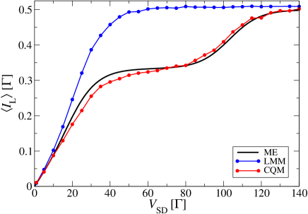
Figure 1: The steady-state current from the left lead ($\langle I_{L}\rangle$) as function of the bias voltage ($V_{\rm SD}$). The black symbols are the results from the QME approach. The blue and red curves correspond to the LMM and CQM, respectively. Parameters used: $\Gamma=2\Gamma_{\rm L}=2\Gamma_{\rm R}=1$, $\epsilon_{\uparrow}=\epsilon{\downarrow}=10\Gamma$, $T=4\Gamma$, $U=40\Gamma$, $\Delta_{\sigma}=0.32$, $N_{\rm tr}=3\times 10^{4}$, and $\mu_{\rm L}=-\mu_{\rm R}=V/2$.

III Complete quasiclassical map (CQM)

For an operator $\hat{A}$, in the Hilbert space of the Anderson impurity model, the Heisenberg equation of motion reads

$$\frac{d\hat{A}}{dt}=i\left[\hat{H}_{0},\hat{A}\right]+iU\left[\hat{n}_{\uparrow},\hat{A}\right]\hat{n}_{\downarrow}+iU\hat{n}_{\uparrow}\left[\hat{n}_{\downarrow},\hat{A}\right].$$ (5)

where $\hat{H}_{0}$,

$$\hat{H}_{0}=\underset{\sigma=\uparrow,\downarrow}{\sum}\varepsilon_{\sigma}\hat{d}_{\sigma}^{\dagger}\hat{d}_{\sigma}+\underset{\underset{k\in\rm L,\rm R}{\sigma=\uparrow,\downarrow}}{\sum}\varepsilon_{k}\hat{c}_{k\sigma}^{\dagger}\hat{c}_{k\sigma}+\underset{\underset{k\in\rm L,\rm R}{\sigma=\uparrow,\downarrow}}{\sum}t_{k}\hat{d}_{\sigma}^{\dagger}\hat{c}_{k\sigma}+{\rm h.c.}$$ (6)

is the one-body, noninteracting part of the Hamiltonian. We wish to find a map for $\hat{A}$ to a function of classical phase-space variables, $A[\vec{R}]$, that would preserve the dynamics $\left<\hat{A}(t)\right>=\left<A(t)\right>_{c}$, where $\left<\hat{A}(t)\right>=\mathrm{Tr}\left(\hat{\rho}\hat{A}(t)\right)$, and

$$\left<A(t)\right>_{c}=\int d\vec{R}\,\rho_{0}(\vec{R})A[\vec{R(t)}]$$ (7)

is the classical expectation value with respect to the initial probability distribution $\rho_{0}$ of the total system. We do this in two parts. First we construct a complete map for quadratic Hamiltonians, which is extendable to any even order operator, and valid for noninteracting fermionic systems. Then, we propose a strategy for mapping Hamiltonians of higher order containing onsite Hubbard interactions. In all the simulations, the equations of motion are solved numerically using an adaptive Rung-Kutta(4,5) method. The number of trajectories, $N_{\rm tr}$, used to converge the results is specified below for each case study. For the steady-state results, additional time averaging is considered.

III.1 Noninteracting fermions

We first consider the case of non-interacting fermions, $U=0$, described by a Hamiltonian that depends quadratically on the creation and annihilation operators, $\hat{H}_{0}$. To reproduce the dynamics of the expectation value of quadratic operators under the evolution describe in Eq. (5) we require:

1. For any quadratic operator $\hat{A}$, and its classical counterpart $A$, the commutator and the Poisson bracket satisfies the correspondence relation $i\left[\hat{H}_{0},\hat{A}\right]=\left\{A,H_{0}\right\}$.

2. For any quadratic expectation value, the initial probability distribution $\rho_{0}$ must satisfy $\left<\hat{A}(0)\right>=\left<A(0)\right>_{c}$, and respect the quantum discrete nature of the occupations.

It is straightforward to show that condition (a) is satisfied by mapping a pair of creation and annihilation operators to a phase space of conjugated variables, $\vec{R}=({x},{p}_{x},{y},{p}_{y})$, as

$$\hat{a}_{n}^{\dagger}\hat{a}_{n} \mapsto x_{n}p_{y,n}-y_{n}p_{x,n},$$ (8)

$$\hat{a}_{n}^{\dagger}\hat{a}_{m} \underset{m\neq n}{\mapsto} \frac{1}{2}\left[i\left(x_{n}p_{x,m}-p_{x,n}x_{m}+y_{n}p_{y,m}-p_{y,n}y_{m}\right)\right.$$

$$+\left.\left(x_{n}p_{y,m}-p_{x,n}y_{m}+x_{m}p_{y,n}-p_{x,m}y_{n}\right)\right],$$

$$\hat{a}_{n}^{\dagger}\hat{a}_{m}^{\dagger} \mapsto \frac{1}{2}\left[i\left(x_{n}p_{x,m}-p_{x,n}x_{m}-y_{n}p_{y,m}+p_{y,n}y_{m}\right)\right.$$

$$-\left.\left(x_{n}p_{y,m}-p_{x,n}y_{m}-x_{m}p_{y,n}+p_{x,m}y_{n}\right)\right],$$

$$\hat{a}_{n}\hat{a}_{m} \mapsto \frac{1}{2}\left[i\left(x_{n}p_{x,m}-p_{x,n}x_{m}-y_{n}p_{y,m}+p_{y,n}y_{m}\right)\right.$$

$$+\left.\left(x_{n}p_{y,m}-p_{x,n}y_{m}-x_{m}p_{y,n}+p_{x,m}y_{n}\right)\right]\,,$$

This identifies positions, $(x,y)$ and their conjugate momenta, $({p}_{x},{p}_{y})$, and the Poisson bracket can be used to check that this map returns the quantum commutator of any pair of quadratic creation/annihilation operators. Because any quadratic Hamiltonian with a set of quadratic operators constitutes a closed Lie algebra of quadratic operators, condition (a) insures a loyal representation of the dynamics in terms of Hamilton’s equations. We note in passing that we subtracted $1/2$ from the classical map of $\hat{n}_{i}\equiv\hat{a}_{i}^{\dagger}\hat{a}_{i}$ to include a Langer-like correctionMiller and McCurdy (1978).

For leads that are in thermal equilibrium and uncorrelated initial state, condition (b) can be satisfied by setting the initial occupation of each mode in the left and right leads to a value 0 or 1, such that the expectation value, averaged over the set of initial conditions, satisfies the Fermi-Dirac distribution.Swenson et al. (2011) Operationally, we choose a random number $\xi_{k\sigma}\in[0,1]$ and then select the occupation of mode $k\sigma$ of the $\ell$-lead according to

$$n_{k\sigma}=\left\{\begin{array}[]{ll}0\quad\xi_{k\sigma}>\left(1+e^{\beta_{\ell}(\epsilon_{k}-\mu_{\ell})}\right)^{-1}\\ 1\quad\xi_{k\sigma}\leq\left(1+e^{\beta_{\ell}(\epsilon_{k}-\mu_{\ell})}\right)^{-1}\end{array}\right.,$$ (9)

where $\beta_{\ell}=1/k_{\rm B}T_{\ell}$ and $\mu_{l}$ are the inverse temperature times Boltzmann’s constant and chemical potential of the $\ell$-lead, respectively. The Cartesian coordinates are then sampled according to Li et al. (2013)

$$x_{k\sigma} = \cos(\theta_{k\sigma}),\quad p_{x,n\sigma}=-n_{k\sigma}\sin(\theta_{k\sigma})$$ (10)

$$y_{k\sigma} = \sin(\theta_{k\sigma}),\quad p_{y,n\sigma}=n_{k\sigma}\cos(\theta_{k\sigma}),$$

where $\theta_{k\sigma}$ is chosen randomly in the interval $[0,2\pi]$ and $n_{k\sigma}=x_{k\sigma}p_{y,k\sigma}-y_{k\sigma}p_{x,k\sigma}$ satisfies Eq. (9), resulting in $\left<\hat{n}_{k\sigma}\right>=\left<n_{k\sigma}\right>_{c}=(1+\exp[\beta_{\ell}(\epsilon_{k}-\mu_{\ell})])^{-1}$ at the initial time. By construction, the expectation value at the initial time is $\left<a_{n}^{\dagger}a_{m}\right>_{c}=\left<a_{n}^{\dagger}a_{m}^{\dagger}\right>_{c}=\left<a_{n}a_{m}\right>_{c}=0$, as expected for averages taken with respect to uncorrelated thermal distribution. The sampling choice in Eq. (10) is not unique, but it does provide an efficient averaging of the expectation values with respect to the number of trajectories.Li et al. (2013) In a similar manner, one can set the initial occupation of the dot.

Comparing the proposed CQM given by Eq. (8) to the LMM, we find that the mappings of the diagonal term $\hat{a}_{n}^{\dagger}\hat{a}_{n}$ and of the linear combination $\hat{a}_{n}^{\dagger}\hat{a}_{m}^{\dagger}+\hat{a}_{m}^{\dagger}\hat{a}_{n}^{\dagger}$ are identical in both maps, but the remaining terms in Eq. (8) cannot be expressed using the LMM. This leads to the Hamiltonian being expressed identically in both maps,

$$H_{0} = \underset{\sigma=\uparrow,\downarrow}{\sum}\varepsilon_{\sigma}\left(x_{\sigma}p_{y,\sigma}-y_{\sigma}p_{x,\sigma}\right)$$

$$+ \underset{\underset{k\in L,R}{\sigma=\uparrow,\downarrow}}{\sum}\varepsilon_{k}\left(x_{k\sigma}p_{y,k\sigma}-y_{k\sigma}p_{x,k\sigma}\right)$$

$$+ \underset{\underset{k\in L,R}{\sigma=\uparrow,\downarrow}}{\sum}t_{k}\left(x_{\sigma}p_{y,k\sigma}-y_{\sigma}p_{x,k\sigma}+x_{k\sigma}p_{y,\sigma}-y_{k\sigma}p_{x,\sigma}\right)\,.$$

For this non-interacting Hamiltonian, mapping $H_{0}$ and then deriving Hamilton’s equations of motion for the phase space variables is identical to deriving Heisnberg’s equation of motion for the bi-linear operators and then mapping the results using Eq. (8).

We can also map other quadratic observables, such as the current from the left lead:

$$\hat{I}_{\rm L} =-\frac{d}{dt}\underset{\underset{k\in\rm L}{\sigma=\uparrow,\downarrow}}{\sum}\hat{c}_{k\sigma}^{\dagger}\hat{c}_{k\sigma}\mapsto$$

$$\underset{\underset{k\in\rm L}{\sigma=\uparrow,\downarrow}}{\sum}t_{k}\left(y_{\sigma}p_{y,k\sigma}-p_{y,\sigma}y_{k\sigma}+x_{\sigma}p_{x,k\sigma}-p_{x,\sigma}x_{k\sigma}\right)\,.$$

As a diagonal term, the above form is also identical to the expression obtained by the LMM.Li et al. (2013) In the upper panel of Fig. 2 we compare the results for the left current generated by the CQM (which in this case are equivalent to the LMM) with exact quantum mechanical results for a noninteracting model Hamiltonian. As expected, the agreement between the CQM (or the LMM) and exact quantum mechanical results is excellent. In the next section we show that for the CQM these result can be extended to higher-order operators.

III.2 Higher order operators

Mapping higher order operators, operators that involve more than one pair of creation/annihilation operators, is more difficult due to the nonlocal character of fermions arising from their exclusion statistics. Ignoring the fermionic nature does not seem to make any significant difference for a single pair of creation/annihilation operators,Swenson et al. (2011); Li et al. (2013) but for higher order operators, the anti-commutation of the creation/annihilation fermionic operators plays a significant role and describing quantum fluctuations such as shot noise requires a careful consideration of this effect.

For example, consider a map for the operator $\hat{A}=a_{n}^{\dagger}a_{m}a_{m}^{\dagger}a_{k}$. Using the anti-commutation nature of $\{a_{n}^{\dagger},a_{n}\}=1$, we can express the expectation value of $\hat{A}$ using four different terms that are identical quantum mechanically, but differ when mapped onto classical phase space variables. Specifically, expanding $\left<\hat{A}\right>$

$$\left<\hat{a}_{n}^{\dagger}\hat{a}_{m}\hat{a}_{m}^{\dagger}\hat{a}_{k}\right>= C_{1}\left<\left(\hat{a}_{n}^{\dagger}\hat{a}_{m}\right)\left(\hat{a}_{m}^{\dagger}\hat{a}_{k}\right)\right>$$

$$+ C_{2}\left<\left(\hat{a}_{n}^{\dagger}\hat{a}_{k}\right)-\left(\hat{a}_{n}^{\dagger}\hat{a}_{m}^{\dagger}\right)\left(\hat{a}_{m}\hat{a}_{k}\right)\right>$$

$$+ C_{3}\left<\left(\hat{a}_{n}^{\dagger}\hat{a}_{k}\right)\left(\hat{a}_{m}\hat{a}_{m}^{\dagger}\right)\right>$$

$$+ C_{4}\left<\delta_{nk}\left(\hat{a}_{m}\hat{a}_{m}^{\dagger}\right)-\left(\hat{a}_{k}\hat{a}_{m}\right)\left(\hat{a}_{m}^{\dagger}\hat{a}_{n}^{\dagger}\right)\right>.$$

we find there are four unique combinations of operators, which generically have coefficients, $C_{i}$. To determine the best choice of $C_{i}$, we impose conditions (a) and (b) of Sec. III.1 on the time evolution of $\hat{A}$ and require that the time evolution of $\hat{A}$ be exact for a quadratic Hamiltonian, i.e., that $i[\hat{H},\hat{A}]=\{A,H\}$ and that $\left<\hat{A}(0)\right>=\left<A(0)\right>_{c}$. For an uncorrelated initial thermal state, the values that satisfy these conditions are $C_{1}=1,C_{2}=-1,C_{3}=1$, and $C_{4}=0$. Note that Eq. (III.2) contains pairs of creation or annihilation operators $(a_{n}^{\dagger}a_{m}^{\dagger}$ or $a_{n}a_{m})$, which cannot be described within the LMM.

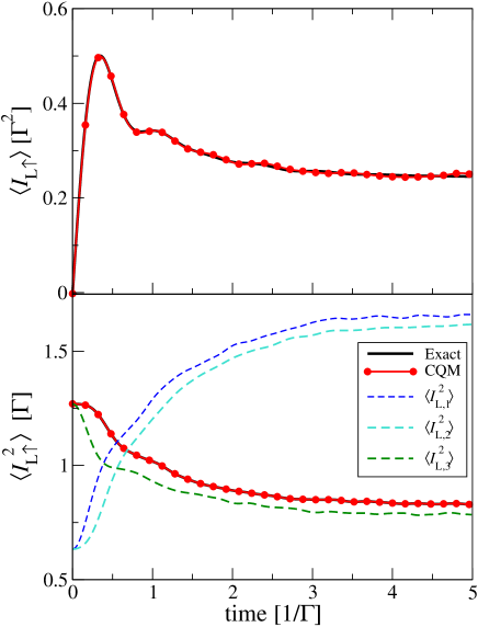
Figure 2: Upper panel: The average left current for spin up ($\langle I_{\rm L\uparrow}(t)\rangle$) as a function of time for a non-interacting model Hamiltonian. The solid black line represents the exact quantum mechanical result Swenson et al. (2011) and a the red symbols are the result of CQM. Lower panel: The average left current squared for spin up ($\langle I^{2}_{\rm L\uparrow}(t)\rangle$) as a function of time. In addition to the exact quantum mechanical (solid black curve) and CQM (red symbols) results, we also show the individual terms $\langle I^{2}_{\rm L,1}(t)\rangle$ (blue), $\langle I^{2}_{\rm L,2}(t)\rangle$ (cyan), and $\langle I^{2}_{\rm L,3}(t)\rangle$ (green). Parameters used: $\Gamma=2\Gamma_{\rm L}=2\Gamma_{\rm R}=1$, $\epsilon_{\uparrow}=\epsilon{\downarrow}=-\Gamma$, $T=\frac{\Gamma}{5}$, $U=0$, $N_{\rm tr}=10^{5}$, and $\mu_{\rm L}=-\mu_{\rm R}=6\Gamma$.

Applying this procedure to the second moment of the left current for the noninteracting Hamiltonian yields a simple expression for $\left<\hat{I}_{\rm L}^{2}\right>=\left<\hat{I}_{\rm L,1}^{2}\right>-\left<\hat{I}_{\rm L,2}^{2}\right>+\left<\hat{I}_{\rm L,3}^{2}\right>$, where

$$\left<\hat{I}_{\rm L,1}^{2}\right> = \underset{\underset{j,k\in L}{\sigma=\uparrow,\downarrow}}{\sum}t_{j}t_{k}\left\langle\left(\hat{c}_{j\sigma}^{\dagger}\hat{d}_{\sigma}\right)\left(\hat{d}_{\sigma}^{\dagger}\hat{c}_{k\sigma}\right)+\left(\hat{d}_{\sigma}^{\dagger}\hat{c}_{j\sigma}\right)\left(\hat{c}_{k\sigma}^{\dagger}\hat{d}_{\sigma}\right)\right\rangle$$

$$\left<\hat{I}_{\rm L,2}^{2}\right> = \underset{\underset{j,k\in L}{\sigma=\uparrow,\downarrow}}{\sum}t_{j}t_{k}\left\langle\left(\hat{c}_{j\sigma}^{\dagger}\hat{c}_{k\sigma}\right)-\left(\hat{c}_{j\sigma}^{\dagger}\hat{d}_{\sigma}^{\dagger}\right)\left(\hat{d}_{\sigma}\hat{c}_{k\sigma}\right)\right.$$

$$+\left.\delta_{jk}\left(\hat{d}_{\sigma}^{\dagger}\hat{d}_{\sigma}\right)-\left(\hat{d}_{\sigma}^{\dagger}\hat{c}_{k\sigma}^{\dagger}\right)\left(\hat{c}_{j\sigma}\hat{d}_{\sigma}\right)\right\rangle$$

$$\left<\hat{I}_{\rm L,3}^{2}\right> = \underset{\underset{j,k\in L}{\sigma=\uparrow,\downarrow}}{\sum}t_{j}t_{k}\left\langle\left(\hat{c}_{j\sigma}^{\dagger}\hat{c}_{k\sigma}\right)\left(\hat{d}_{\sigma}\hat{d}_{\sigma}^{\dagger}\right)+\left(\hat{d}_{\sigma}^{\dagger}\hat{d}_{\sigma}\right)\left(\hat{c}_{j\sigma}\hat{c}_{k\sigma}^{\dagger}\right)\right\rangle.$$

As can be shown explicitly, this mapping of the second moment of the left current operator satisfies both conditions (a) and (b).

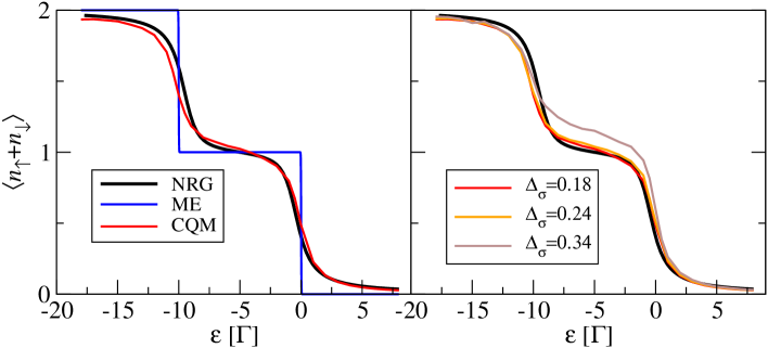
Figure 3: Left panel: The steady-state quantum dot population as a function of the gate voltage $\varepsilon=\varepsilon_{\uparrow}=\varepsilon_{\downarrow}$ under equilibrium conditions ($\mu_{L}=\mu_{R}=0$). Right panel: The dependence of the steady-state dot population on the choice of the value of $\Delta_{\sigma}$ (cf., Eq. (15)). Parameters used: $\Gamma=2\Gamma_{L}=2\Gamma_{R}=1$, $T=\Gamma/100$, $U=10\Gamma$, $N_{\rm tr}=3\cdot 10^{4}$, and for the left panel: $\Delta_{\sigma}=0.18$.

In the bottom panel of Fig. 2 we show the time evolution of $\left<\hat{I}_{\rm L}^{2}\right>$ for a quadratic Hamiltonian where $U=0$. The agreement between the exact quantum mechanical result and the CQM is excellent. We also plot the individual terms $\left<\hat{I}_{\rm L,1}^{2}\right>$, $\left<\hat{I}_{\rm L,2}^{2}\right>$, and $\left<\hat{I}_{\rm L,3}^{2}\right>$ (dashed lines). Only the proper combination of all three terms yields an accurate description of $\left<\hat{I}_{\rm L}^{2}\right>$. We note that the LMM can only be used to map the first term, but not the other two that contribute to $\left<\hat{I}_{\rm L}^{2}\right>$.

III.3 Interacting fermions

The on-site interaction, $U\hat{n}_{\uparrow}\hat{n}_{\downarrow}$, that manifest the Coulomb blockade effect, is a four index term that is outside the space defined by the CQM. In order to account for this two-body interaction term, we map the two terms proportional to $U$ in Eq. (5) according to

$$iU\left[\hat{n}_{\uparrow},\hat{A}\right]\hat{n}_{\downarrow}\mapsto U\left\{A_{c},n_{\uparrow}\right\}\theta\left(n_{\downarrow}-\Delta_{\downarrow}\right)$$ (15)

$$iU\hat{n}_{\uparrow}\left[\hat{n}_{\downarrow},\hat{A}\right]\mapsto U\left\{A_{c},n_{\downarrow}\right\}\theta\left(n_{\uparrow}-\Delta_{\uparrow}\right),$$

where $\theta$ is the Heaviside step function. The idea behind this choice is that the term $U\hat{n}_{\uparrow}\hat{n}_{\downarrow}$ contributes to the dynamics only when both electrons with spin up and spin down occupy the site. Classically, the occupation number admits a continuous value, which implies that the Hubbard term can become significant for fractional populations of the two spin-channels. Much like a mean-field approximation, these fraction contributions of the Hubbard term will smear the Coulomb blockade effect. By introducing the step function, we impose that contributions to the dynamics from the Hubbard term arise only in trajectories for which $n_{\uparrow(\downarrow)}>\Delta_{\uparrow(\downarrow)}$. The parameter $\Delta_{\uparrow(\downarrow)}$ is determined according to the distribution of $n_{\uparrow(\downarrow)c}$ and will be discussed in detail below. We note that the classical expression in Eq. (15) is not derivable from a Hamiltonian, and therefore does not in principle conserve energy or the norm of phase space. Nevertheless, we find relaxation to an intermediate time, long lived steady-state for all of the observables studied on timescales shorter than the recurrence times.

Considering the Anderson impurity model, the equations of motion for the Cartesian variables for the lead degrees of freedom are

$$\dot{x}_{j\sigma} = -\epsilon_{j}y{}_{j\sigma}-t_{j}y_{\sigma},$$ (16)

$$\dot{y}_{j\sigma} = \epsilon_{j}x{}_{j\sigma}+t_{j}x_{\sigma},$$

$$\dot{p}_{x,j\sigma} = -\epsilon_{j}p_{y,j\sigma}-t_{j}p_{y,\sigma},$$

$$\dot{p}_{y,j\sigma} = \epsilon_{j}p_{x,j\sigma}+t_{j}p_{x,\sigma},$$

and those for the system’s degrees of freedom are

$$\dot{x}_{\sigma} = -\epsilon_{\sigma}y_{\sigma}-\sum_{k\in L,R}t_{k}y_{k\sigma}-Uy_{\sigma}\theta\left(n_{\bar{\sigma}}-\Delta_{\bar{\sigma}}\right),$$ (17)

$$\dot{y}_{\sigma} = \epsilon_{\sigma}x_{\sigma}+\sum_{k\in L,R}t_{k}x_{k\sigma}+Ux_{\sigma}\theta\left(n_{\bar{\sigma}}-\Delta_{\bar{\sigma}}\right),$$

$$\dot{p}_{x,\sigma} = -\epsilon_{\sigma}p_{y,\sigma}-\sum_{k\in L,R}t_{k}p_{y,k\sigma}-Up_{y,\sigma}\theta\left(n_{\bar{\sigma}}-\Delta_{\bar{\sigma}}\right),$$

$$\dot{p}_{y,\sigma} = \epsilon_{\sigma}p_{x,\sigma}+\sum_{k\in L,R}t_{k}p_{x,k\sigma}+Up_{x,\sigma}\theta\left(n_{\bar{\sigma}}-\Delta_{\bar{\sigma}}\right),$$

where $\bar{\sigma}=\downarrow,\uparrow$ is the opposite spin to $\sigma=\uparrow,\downarrow$.

In Fig. 1 we plot the I-V curve obtained by the CQM and compare it to the QME in Ref. Levy et al., 2019 and to the results obtained by the LMM. We consider the limit of weak system-bath coupling and high temperature where the QME provides a good approximation for the dynamics of the system. The LMM provides a good description of the I-V characteristics at low and high bias voltages, but it fails to capture the staircase structure reminiscent of the Coulomb blockade. The CQM reproduce the QME results quantitatively, specifically, it captures the staircase structure due to the Coulomb blockade effect. In this high temperature regime, the agreement between the CQM and the quantum mechanical results is observed for a wide range of onsite Hubbard repulsion term and also for the quantum dot population.

Next, we consider a regime where the QME breaks down, namely, the low temperature regime. For simplicity we focus on the equilibrium case where $\mu_{L}=\mu_{R}=0$. In this regime, solutions for the population as function of the gate voltage ($\varepsilon=\varepsilon_{\uparrow}=\varepsilon_{\downarrow}$) are readily available using the numerical renormalization group (NRG) technique.Bulla, Costi, and Pruschke (2008b); Dou, Miao, and Subotnik (2017) In the left panel of Fig. 3 we plot the quantum dot total population ($\langle n_{\uparrow}+n_{\downarrow}\rangle$) as a function of the gate voltage. The NRG results show a staircase shape which is a manifestation of the Coulomb blockade effect. The CQM agrees quantitatively with the NRG results over a wide range of gate voltages. Specifically, it captures both the position of the blockade as well as its width. The QME approach, however, captures only the position of the resonances; the broadening of the transitions are missing completely. This qualitative difference between the CQM and QME approaches signifies the advantages of the quasiclassical mapping techniques over the commonly used QME approach for a broad range of temperatures.

The mapping of the Hubbard term in Eq. (15) introduces a parameter, $\Delta_{\uparrow(\downarrow)}$, which is determined self-consistently. For the results show in Fig. 3 we use a single value for $\Delta_{\sigma}=0.18$, determined by considering the particle-hole symmetry point, where $\varepsilon_{\uparrow}=\varepsilon_{\downarrow}=-U/2$. At the symmetric point, the steady state value of the average dot populations is $\left<\hat{n}_{\sigma}\right>=1/2$. Since quantum mechanically $\hat{n}_{\sigma}$ can only assume two value, $0$ or $1$, whereas the distribution of $n_{\sigma}$ is continuous, to obtain an average dot population $\left<\hat{n}_{\sigma}\right>=1/2$, we set $\Delta_{\sigma}$ to the median of the distribution of values of $n_{\sigma}$. This ensures that the Hubbard terms in Eq. (15) are significant only when $n_{\sigma}$ is sufficiently large, modeling the discrete nature of the spin-dependent dot occupations.

In the right panel of Fig. 3 we show the results obtained for the total dot occupation for different values of $\Delta_{\sigma}$. Only $3$ iterations are required to converge the results for $\Delta_{\sigma}$. We start with an initial guess of $\Delta_{\sigma}=0.34$. In the next iteration, we set $\Delta_{\sigma}$ to the new median of the distribution of values of $n_{\sigma}$, in this case $\Delta_{\sigma}=0.24$. We then repeat this procedure until convergence (only one more iteration is required). The results clearly show that the expectation value is not very sensitive to small variations in the value of $\Delta_{\sigma}$, but the converged results provide the best agreement with the NRG results.

The agreement between the CQM and the quantum mechanical results are not limited to steady-state properties. In fact, our mapping also captures quantitatively the hallmarks of the Coulomb blockade in the relaxation towards the steady state. Shown in Fig. 4 is the time dependence of the dot occupation for two different values of $U$, with a bias voltage of $V_{\rm SD}=\mu_{\rm L}-\mu_{\rm R}=\Gamma$, and temperature $T=\Gamma$. Here we compare the CQM to numerically converged real-time stochastically sampled diagrammatic techniques applied within the reduced density matrix formalism.Cohen and Rabani (2011) For both values of $U$ we find that the full time dependence is in good agreement with the numerically converged data. In each case, the dot population increases monotonically and the timecales required to reach the long time limit are comparable.

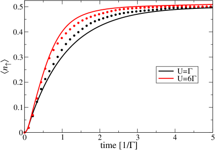
Figure 4: Comparison of the dot population ($\langle n_{\uparrow}+n_{\downarrow}\rangle$) derivative from the memory-kernel formalism Cohen and Rabani (2011) (solid lines) and the CQM approach (dot symbols) for an initially unoccupied dot for two values of the interaction energy ($U=\Gamma$ and $U=6\Gamma$). Parameters used: $\Gamma=2\Gamma_{\rm L}=2\Gamma_{\rm R}=1$, $T=\Gamma$, $\mu_{\rm L}=-\mu_{\rm R}=\Gamma/2$, $\varepsilon_{\uparrow}=\varepsilon_{\downarrow}=-U/2$, $N_{\rm tr}=6\times 10^{4}$, and for the CQM results; $\Delta_{\sigma}=0.24$ for $U=6\Gamma$, and $\Delta_{\sigma}=0.31$ for $U=\Gamma$.

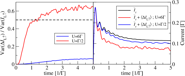
Figure 5: Left panel: The ratio of the variances of the left currents for spin up as a function of time. The red line is for $U=6\Gamma$ and the blue for $U=\Gamma/2$. Computational superiority is observed below the threshold ratio $1/2$ noted by the black dashed line. Right panel: The black line is the exact reference current $(U=0)$, the red and blue line are the currents obtained using a reference system for $U=6\Gamma$ and $U=\Gamma$, respectively. The parameters are: $\Gamma=2\Gamma_{\rm L}=2\Gamma_{\rm R}=1$, $T=0.5\Gamma$, $\varepsilon_{\uparrow}=\varepsilon_{\downarrow}=2\Gamma$, $N_{\rm tr}=3\times 10^{4}$, and $\mu_{\rm L}=-\mu_{\rm R}=2\Gamma$.

IV Reference dynamics for statistical convergence

When evaluating the classical expected value Eq. (7), the integral over the initial distribution is replaced by averaging over different initial configurations of the leads that satisfy the Fermi-Dirac distribution. For a large number of initial conditions, $N_{\rm tr}$, the procedure converges to the desired distribution and to the exact expectation value. However, the low dimensional nearly harmonic system generically requires a large number of initial conditions to statistically converge the result. To reduce the number of initial conditions for a given statistical error, we introduce a reference system whose expectation value can be determined exactly and inexpensively. Specifically, the expectation value of an observable $A$ is calculated according to

$$\left<A\right>=\left<A_{\mathrm{r}}-A_{\mathrm{r}}+A\right>=\bar{A}_{\mathrm{r}}+\left<\Delta A\right>$$ (18)

where $A_{\mathrm{r}}$ is an observable used as the reference, and $\bar{A}_{\mathrm{r}}$ is the exact expectation value of $A_{\mathrm{r}}$ evaluated using a different inexpensive method. In the limit $N_{\rm tr}\rightarrow\infty$ we have $\left<A_{\mathrm{r}}\right>\rightarrow\bar{A}_{\mathrm{r}}$ and $\left<A\right>$ will approach the real expectation value. However, for a finite $N_{\rm tr}$, and a smart choice of $A_{\mathrm{r}}$, one can reduce significantly the statistical error of this estimator. This is clarified by considering the variance using the reference system

$$\text{Var}(\Delta A)=\text{Var}(A)+\text{Var}(A_{\mathrm{r}})-2\text{Cov}(A,A_{\mathrm{r}}).$$ (19)

If $A$ and $A_{\mathrm{r}}$ are correlated, it is possible to have $\text{Var}(\Delta A)<\text{Var}(A)$. As we are now propagating both $A$ and $A_{\mathrm{r}}$, to reduce the computational effort we desire that

$$\frac{\text{Var}(\Delta A)}{\text{Var}(A)}<\frac{1}{2}.$$ (20)

Given that the sample variance reduces as $1/N_{\rm tr}$, to obtain computational superiority the ratio in Eq.(20) is bounded by 1/2. However, improvement in the computational effort can already be seen for ratios that are above this factor, since typically propagation of the reference system is not as costly as of the system of interest. Non-interacting or mean-field Hamiltonians that can be solved analytically serve as examples of reference systems that can reduce noise for the dynamics of interacting systems. Other possibilities include considering dynamics that are generated from some effective Hamiltonian with the same initial configurations.

Shown in Fig. 5 are two examples, one in which the reference system method works good and one in which it fails. On the left panel we plot the ratio of the variances of the left current with spin up as a function of time, and on the right we plot the corresponding currents. The reference considered here is the current calculated for noninteracting systems where an exact solution can be obtained by direct diagonalization of the single-particle Hamiltonian. We see that when the reference current, $\bar{I}_{\rm r}$, becomes very different from the real current, $\bar{I}_{\rm r}+\left<\Delta I\right>$, (for $U=6\Gamma$ in the figure) the ratio of the variances at steady-state exceeds its bound $1/2$. However, when the reference and the real currents are proximate but still quite different (for $U=\Gamma/2$ in the figure), we see that the ratio of the variances is reduced significantly as a consequence of correlations between the trajectories of the currents.

We note that for parameter regime where the reference and real currents almost coincide the fluctuations drastically decreased, the ratio of the variances at steady state reaches as low as $\sim 10^{-4}$. This implies that for a fixed statistical convergence threshold, the number of initial conditions decreases by two orders of magnitude, since each estimate is statistically independent. One can also note that at short times the reference system always reduces the fluctuations significantly. The reason is that we used an uncorrelated initial condition and thus the short time behavior is set by $\sim\Gamma^{-1}$. It takes a certain amount of time for correlations to build up and for the interacting part in the Hamiltonian to influence the dynamics, yielding a statistical benefit for short times even when the steady-state result is far from the noninteracting limit.

The idea of using a reference system can be extended beyond the description above. For example, if one wishes to calculate the current as function of $U$, one can start the evaluation for small $U$ and increase it “adiabatically”. For each calculation of the current, the previous current (with smaller $U$) can be used as the reference system. Of course, the exact term in Eq. (18) is no longer exact and carry with it some error, but this can still be beneficial, as trajectories of the different currents are likely to be correlated given that the change in $U$ is small.

V conclusions

We have presented a quasiclassical method to simulate nonequilibrium dynamics of interacting fermions. We have constructed this map using the correspondence relation between the commutator and the Poisson bracket, in order to preserve Heisenberg’s equation of motion for one-body operators. We have shown that this classical map is complete for quadratic expectation values under quadratic Hamiltonians and it can be extended to higher moments accurately. This feature makes the study of fluctuations and higher-order correlations accessible.

For interacting systems, the dynamics is approximated by mapping the equation of motion and enforcing a quantization rule that determines for which values of $n_{\sigma}$ the dynamics is influenced by the Hubbard term. This, together with a quasiclassical initial distribution, provides a quantitative agreement with other methods in regimes where those other methods are known to be accurate. Thus, a quantitative description of nonequilibrium currents in the Anderson model, including their steady-state behavior as illustrated by the presence of the Coulomb blockade, their fluctuations as encodes in the second moment of the current, and the relaxation of each to their steady state can be obtained.

We have also shown a way to enhance the statistical convergence of this method by introducing a reference system, whose dynamics can be computed exactly, and averaging the difference between the reference system and the system of interest. Provided the reference system is correlated with the system of interest, fluctuations are reduced in the averaging procedure, and we have shown that this can increase the computational efficiency by up to 2 orders of magnitude over naive sampling. Together, these results make the quasiclassical method appealing for studying nonequilibrium phenomena in complex chemical systems. Indeed, realistic systems of molecular junctions routinely operate a low effective temperatures, and finite interaction strengths rendering other low scaling approximate approaches inaccurate. The method we have presented here is capable of probing these regimes, at a small computational cost that scales linearly in the system degrees of freedom. This should enable studies in correlated transport behavior in high dimensional, molecular systems, far from equilibrium.

Appendix: Relation to quaternion maps

The LMMLi and Miller (2012); Li et al. (2013) is based on expressing the fermionic creation and annihilation operators in terms of a set of quaternions:

$$\hat{a}^{\dagger}=\frac{1}{2}(\sqrt{-1}~{}\hat{\text{i}}-\hat{\text{j}})$$ (21)

$$\hat{a}=\frac{1}{2}(\sqrt{-1}~{}\hat{\text{i}}+\hat{\text{j}}).$$

The quaternions operators $\hat{\text{i}},\hat{\text{j}}$ and $\hat{\text{k}}$ satisfy the anti-commutation relation:

$$\hat{\text{i}}\hat{\text{j}} = -\hat{\text{j}}\hat{\text{i}}=\hat{\text{k}},\quad\hat{\text{j}}\hat{\text{k}}=-\hat{\text{k}}\hat{\text{j}}=\hat{\text{i}},\quad\hat{\text{k}}\hat{\text{i}}=-\hat{\text{i}}\hat{\text{k}}=\hat{\text{j}}$$ (22)

$$\hat{\text{i}}^{2} = \hat{\text{j}}^{2}=\hat{\text{k}}^{2}=-1.$$

Using the relations in Eqs. (21) and (22), quadratic creation and annihilation operators can be expressed as:

$$\hat{a}_{n}^{\dagger}\hat{a}_{n} = \frac{1}{2}+\frac{\sqrt{-1}}{2}\hat{\text{i}}_{n}\hat{\text{j}}_{n}$$ (23)

$$\hat{a}_{n}^{\dagger}\hat{a}_{m} = \frac{1}{4}\left(-\hat{\text{i}}_{n}\hat{\text{i}}_{m}-\hat{\text{j}}_{n}\hat{\text{j}}_{m}+\sqrt{-1}~{}\left(\hat{\text{i}}_{n}\hat{\text{j}}_{m}+\hat{\text{i}}_{m}\hat{\text{j}}_{n}\right)\right)$$

$$\hat{a}_{n}^{\dagger}\hat{a}_{m}^{\dagger} = \frac{1}{4}\left(-\hat{\text{i}}_{n}\hat{\text{i}}_{m}+\hat{\text{j}}_{n}\hat{\text{j}}_{m}-\sqrt{-1}~{}\left(\hat{\text{i}}_{n}\hat{\text{j}}_{m}-\hat{\text{i}}_{m}\hat{\text{j}}_{n}\right)\right)$$

$$\hat{a}_{n}\hat{a}_{m} = \frac{1}{4}\left(-\hat{\text{i}}_{n}\hat{\text{i}}_{m}+\hat{\text{j}}_{n}\hat{\text{j}}_{m}+\sqrt{-1}~{}\left(\hat{\text{i}}_{n}\hat{\text{j}}_{m}-\hat{\text{i}}_{m}\hat{\text{j}}_{n}\right)\right)$$

The commutation relation of two elementary quaternions are then mapped to a cross product of vectors in phase space,

$$\sqrt{\frac{-1}{2}}~{}\hat{\text{i}}\rightarrow\textbf{r}=\left(\begin{array}[]{c}x\\ y\end{array}\right),\quad\sqrt{\frac{1}{2}}~{}\hat{\text{j}}\rightarrow\textbf{p}=\left(\begin{array}[]{c}p_{x}\\ p_{y}\end{array}\right).$$ (24)

The CQM replaces the map in Eq.(24) with

$$\sqrt{\frac{\sqrt{-1}}{2}}~{}\hat{\text{i}}\rightarrow u=\left(\begin{array}[]{c}x\\ p_{x}\end{array}\right),\quad\sqrt{\frac{\sqrt{-1}}{2}}~{}\hat{\text{j}}\rightarrow v=\left(\begin{array}[]{c}y\\ p_{y}\end{array}\right).$$ (25)

This choice implies that

$$\frac{\sqrt{-1}}{2}~{}\hat{\text{i}}_{n}\hat{\text{j}}_{m} \rightarrow u_{n}\times v_{m}=x_{m}p_{ym}-p_{xn}y_{m}$$ (26)

$$\frac{\sqrt{-1}}{2}~{}\hat{\text{i}}_{n}\hat{\text{i}}_{m} \rightarrow u_{n}\times u_{m}=x_{m}p_{xm}-p_{xn}x_{m}\quad\forall n\neq m$$

$$\frac{\sqrt{-1}}{2}~{}\hat{\text{j}}_{n}\hat{\text{j}}_{m} \rightarrow v_{n}\times v_{m}=y_{m}p_{ym}-p_{yn}y_{m}\quad\forall n\neq m,$$

and $\frac{\sqrt{-1}}{2}~{}\hat{\text{i}}\hat{\text{i}}=\frac{\sqrt{-1}}{2}~{}\hat{\text{j}}\hat{\text{j}}=-\frac{\sqrt{-1}}{2}$ for $n=m$. The LMM given by Eq. (24) can be used to map the terms $\hat{a}_{n}^{\dagger}\hat{a}_{n}$ and $\hat{a}_{n}^{\dagger}\hat{a}_{m}+\hat{a}_{m}^{\dagger}\hat{a}_{n}$. The CQM extend this to terms like $\hat{a}_{n}^{\dagger}\hat{a}_{m}^{\dagger}$, $\hat{a}_{n}\hat{a}_{m}$ and $\hat{a}_{n}^{\dagger}\hat{a}_{m}$.

References

- Mühlbacher (2008) L. Mühlbacher, Phys. Rev. Lett. 100, 176403 (2008).
- Weiss et al. (2008) S. Weiss, J. Eckel, M. Thorwart, and R. Egger, Phys. Rev. B 77, 195316 (2008).
- Schiró and Fabrizio (2009) M. Schiró and M. Fabrizio, Phys. Rev. B 79, 153302 (2009).
- Werner, Oka, and Millis (2009) P. Werner, T. Oka, and A. J. Millis, Phys. Rev. B 79, 035320 (2009).
- Gull, Reichman, and Millis (2010) E. Gull, D. R. Reichman, and A. J. Millis, Phys. Rev. B 82, 075109 (2010).
- Segal, Millis, and Reichman (2010) D. Segal, A. J. Millis, and D. R. Reichman, Phys. Rev. B 82, 205323 (2010).
- Cohen and Rabani (2011) G. Cohen and E. Rabani, Phys. Rev. B 84, 075150 (2011).
- Härtle et al. (2013) R. Härtle, G. Cohen, D. Reichman, and A. Millis, Phys. Rev. B 88, 235426 (2013).
- Cohen et al. (2015) G. Cohen, E. Gull, D. R. Reichman, and A. J. Millis, Phys. Rev. Lett. 115, 266802 (2015).
- Schmitteckert (2004) P. Schmitteckert, Phys. Rev. B 70, 121302 (2004).
- Anders and Schiller (2005) F. B. Anders and A. Schiller, Phys. Rev. Lett. 95, 196801 (2005).
- Bulla, Costi, and Pruschke (2008a) R. Bulla, T. A. Costi, and T. Pruschke, Rev. Mod. Phys. 80, 395 (2008a).
- Wang and Thoss (2018) H. Wang and M. Thoss, Chem. Phys. 509, 13 (2018).
- Balzer et al. (2015) K. Balzer, Z. Li, O. Vendrell, and M. Eckstein, Phys. Rev. B 91, 045136 (2015).
- Schinabeck et al. (2016) C. Schinabeck, A. Erpenbeck, R. Härtle, and M. Thoss, Phys. Rev. B 94, 201407 (2016).
- Wilner et al. (2013) E. Y. Wilner, H. Wang, G. Cohen, M. Thoss, and E. Rabani, Phys. Rev. B 88, 045137 (2013).
- Wilner et al. (2014a) E. Y. Wilner, H. Wang, M. Thoss, and E. Rabani, Phys. Rev. B 90, 115145 (2014a).
- Wilner et al. (2014b) E. Y. Wilner, H. Wang, M. Thoss, and E. Rabani, Phys. Rev. B 89, 205129 (2014b).
- Datta (1990) S. Datta, J. Phys. C 2, 8023 (1990).
- Harbola, Esposito, and Mukamel (2006) U. Harbola, M. Esposito, and S. Mukamel, Phys. Rev. B 74, 235309 (2006).
- Leijnse and Wegewijs (2008) M. Leijnse and M. R. Wegewijs, Phys. Rev. B 78, 235424 (2008).
- Esposito and Galperin (2009) M. Esposito and M. Galperin, Phys. Rev. B 79, 205303 (2009).
- Esposito and Galperin (2010) M. Esposito and M. Galperin, J. Phys. Chem. C 114, 20362 (2010).
- Dou, Nitzan, and Subotnik (2015) W. Dou, A. Nitzan, and J. E. Subotnik, J. Chem. Phys. 142, 234106 (2015).
- Dorda et al. (2015) A. Dorda, M. Ganahl, H. G. Evertz, W. von der Linden, and E. Arrigoni, Phys. Rev. B 92, 125145 (2015).
- Hettler, Kroha, and Hershfield (1998) M. H. Hettler, J. Kroha, and S. Hershfield, Phys. Rev. B 58, 5649 (1998).
- Datta (2000) S. Datta, Superlattices and Microstructures 28, 253 (2000).
- Xue, Datta, and Ratner (2002) Y. Q. Xue, S. Datta, and M. A. Ratner, Chem. Phys. 281, 151 (2002).
- Galperin, Ratner, and Nitzan (2007) M. Galperin, M. A. Ratner, and A. Nitzan, J. Phys.: Condens. Matter 19, 103201 (2007).
- Haug and Jauho (2008) H. Haug and A.-P. Jauho, Quantum kinetics in transport and optics of semiconductors, 2nd ed., Springer series in solid-state sciences, (Springer, Berlin ; New York, 2008) pp. xix, 360 p.
- Stefanucci and Leeuwen (2013) G. Stefanucci and R. v. Leeuwen, Nonequilibrium Many-Body Theory of Quantum Systems: A Modern Introduction (Cambridge University Press, 2013).
- Mayer and Miller (1979) H.-D. Mayer and W. H. Miller, J. Phys. Chem. 70, 3214 (1979).
- Miller and White (1986) W. H. Miller and K. A. White, J. Chem. Phys. 84, 5059 (1986).
- Van Voorhis and Reichman (2004) T. Van Voorhis and D. R. Reichman, J. Chem. Phys. 120, 579 (2004).
- Miller (2006) W. H. Miller, J. Chem. Phys. 125, 132305 (2006).
- Swenson et al. (2011) D. W. Swenson, T. Levy, G. Cohen, E. Rabani, and W. H. Miller, J. Chem. Phys. 134, 164103 (2011).
- Swenson, Cohen, and Rabani (2012) D. W. Swenson, G. Cohen, and E. Rabani, Mol. Phys. 110, 743 (2012).
- Li and Miller (2012) B. Li and W. H. Miller, J. Chem. Phys. 137, 154107 (2012).
- Li et al. (2013) B. Li, T. J. Levy, D. W. Swenson, E. Rabani, and W. H. Miller, J. Chem. Phys. 138, 104110 (2013).
- Li et al. (2014) B. Li, W. H. Miller, T. J. Levy, and E. Rabani, J. Chem. Phys. 140, 204106 (2014).
- Davidson, Sels, and Polkovnikov (2017) S. M. Davidson, D. Sels, and A. Polkovnikov, Ann. Phys. 384, 128 (2017).
- Montoya-Castillo and Markland (2018) A. Montoya-Castillo and T. E. Markland, Scientific reports 8, 12929 (2018).
- Ray, Chan, and Limmer (2018) U. Ray, G. K.-L. Chan, and D. T. Limmer, J. Chem Phys. 148, 124120 (2018).
- Herman and Kluk (1984) M. F. Herman and E. Kluk, Chem. Phys. 91, 27 (1984).
- Kay (1994) K. G. Kay, J. Chem. Phys. 101, 2250 (1994).
- Stock and Thoss (1997) G. Stock and M. Thoss, Phys. Rev. Lett. 78, 578 (1997).
- Anderson (1961) P. W. Anderson, Phys. Rev. 124, 41 (1961).
- Miller and McCurdy (1978) W. Miller and C. McCurdy, J. Chem. Phys. 69, 5163 (1978).
- Levy et al. (2019) A. Levy, L. Kidon, D. T. Limmer, and E. Rabani, arXiv preprint arXiv:1901.04315 (2019).
- Bulla, Costi, and Pruschke (2008b) R. Bulla, T. A. Costi, and T. Pruschke, Rev. Mod. Phys. 80, 395 (2008b).
- Dou, Miao, and Subotnik (2017) W. Dou, G. Miao, and J. E. Subotnik, Phy. Rev. Lett. 119, 046001 (2017).