Travel time tomography with formally determined incomplete data in 3D
Abstract
For the first time, a globally convergent numerical method is developed and Lipschitz stability estimate is obtained for the challenging problem of travel time tomography in 3D for formally determined incomplete data. The semidiscrete case is considered meaning that finite differences are involved with respect to two out of three variables. First, Lipschitz stability estimate is derived, which implies uniqueness. Next, a weighted globally strictly convex Tikhonov-like functional is constructed using a Carleman-like weight function for a Volterra integral operator. The gradient projection method is constructed to minimize this functional. It is proven that this method converges globally to the exact solution if the noise in the data tends to zero.
Key words. inverse kinematic problem; Carleman-like estimate for the Volterra operator; Lipschitz stability; convexification; globally convergent numerical method
AMS Classification 35R30
1 Introduction
We construct a globally convergent numerical method for the challenging 3D travel time tomography problem (TTTP) with formally determined incomplete data. The TTTP was first considered by Herglotz [7] in 1905 and then by Wiechert and Zoeppritz [34] in 1907 in the 1D case due to a geophysical application, also, see a detailed description of the 1D case in [24]. However, globally convergent numerical methods for the 3D TTTP with formally determined data were not developed so far. By the definition of, e.g. [1, 2], a numerical method for a nonlinear problem is called globally convergent if there exists a theorem claiming that this method delivers at least one point in a sufficiently small neighborhood of the correct solution without relying on any advanced knowledge of this neighborhood, i.e. a good first guess for the solution is not required.
In this paragraph, we indicate those ideas for the TTTP, which are presented here for the first time. More details about the latter statement, including some references, are given in this section below. Since we develop a numerical method, we are allowed to work here with an approximate mathematical model. We study the case when the data for the TTTP are both formally determined and incomplete. The TTTP is considered in the semidiscrete form, i.e. we consider the practically important case of finite differences with respect to two out of three variables, also see Remark 6.1 in section 6. The Lipschitz stability estimate is obtained, which implies uniqueness. Next, the exact solution is constructed via introducing a sequence, which converges to that solution starting from an arbitrary point of a certain bounded set, provided that the noise in the data tends to zero. Since no restrictions are imposed on the size of that set, then this is a globally convergent numerical method. To construct that method, we introduce a weighted Tikhonov-like functional for the TTTP, which is strictly convex on that bounded set, i.e. we use the so-called “convexification” procedure. However, while in all previous versions of the convexification the so-called Carleman Weight Function (CWF) was applied to differential operators, in the current paper the CWF is applied to a Volterra-like nonlinear integral operator. Our method does not use sophisticated geometrical properties to construct the above sequence. Rather, we straightforwardly minimize the above mentioned globally strictly convex Tikhonov-like functional.
The TTTP is the problem of the recovery of the spatially distributed speed of acoustic waves from first times of arrival of those waves. Another well known term for the TTTP is the “inverse kinematic problem of seismic” [24]. Waves are originated by some point sources located on the boundary of the domain of interest. First times of arrival are recorded on a number of detectors located on that boundary. It is well known that the TTTP is actually a nonlinear problem of the integral geometry, see, e.g. [24]. The TTTP has important applications in geophysics [7, 24, 33, 34]. In addition, it was established in [15] that the TTTP arises in the phaseless inverse problem of scattering of electromagnetic waves at high frequencies. The specific TTTP considered here has potential applications in geophysics, checking the bulky baggage in airports, search for possible defects inside the walls, etc..
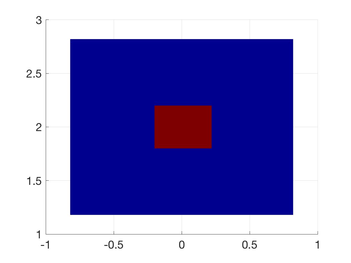
The “formally determined data” means that the number of free variables in the data equals to the number of free variables in the unknown coefficient, . If, however, , then the data are overdetermined. In our case . In the 2D case all previously known results for the TTTP work with formally determined data with . Only complete data for the TTTP were considered in the past. In the 3D case those data were overdetermined with . Complete data for the TTTP are generated by the point source running along the entire surface of the boundary of the domain of interest. Unlike these, our point source runs along an interval of a straight line located outside of the domain of interest. This means that the data are incomplete. The sole purpose of Figure 1 is to illustrate this for a simple case when geodesics are straight lines.
Our approximate mathematical model consists of two items, see Remarks 6.2, 6.3 in the end of section 6 for more details. First, we consider a semidiscrete model. This means that partial derivatives with respect to two out of three variables are written in finite differences. The author believes that this might be valuable for a possible future numerical implementation of the method of this paper. Second, we assume that a certain function generated by the solution of the eikonal equation can be represented as a truncated Fourier series with respect to a special orthonormal basis in the space. That basis was first constructed in [16]. Functions of that basis depend only on the position of the source. The number of terms of this series is not allowed to tend to the infinity. We note that such assumptions quite often take place in the theory of ill-posed problems, and corresponding computational results are not affected by these assumptions, see, e.g. [18, 19, 20], where the same basis was used to obtain good quality numerical results.
The TTTP is about the reconstruction of the right hand side of the nonlinear eikonal Partial Differential Equation (PDE) from boundary measurements of the solution of this equation. It is well known that conventional least squares cost functionals for nonlinear inverse problems are non convex. The non convexity, in turn causes the well known phenomenon of multiple local minima and ravines of that functional, see, e.g. [27] for a quite convincing numerical example. Therefore, convergence of any minimization algorithm to the correct solution is in question, unless its starting point is chosen to be in a sufficiently small neighborhood of that solution, which is the so-called small perturbation approach. However, it is unclear in many applications how to actually obtain that sufficiently small neighborhood.
To avoid the phenomenon of local minima, we apply the so-called convexification method. More precisely, we construct a weighted globally strictly convex Tikhonov-like functional for our TTTP. The key element of this functional is the presence in it of the weight function which looks similar with the CWF.
The convexification was first proposed in [11, 12]. However, those initial works lacked some important analytical results, which would allow numerical studies. Such results were recently obtained in [1]. Thus, recent publications [17, 18, 19] contain both the theory and numerical results for the convexification method for some coefficient inverse problems for PDEs, although not for the TTTP. We prove the global convergence to the correct solution of the gradient projection method of the minimization of our functional.
As to the numerical methods for the TTTP in the D case, , such a method for the 2D TTTP was published in [28]. Another numerical approach in 3D was published in [35]. Both publications [28, 35] use, at a certain stage, the minimization of a least squares cost functional. Since the convexity of those functionals of [28, 35] is not proven, then the problem of local minima is not addressed there. In both publications [28, 35] complete data are used, and these data are overdetermined ones in the 3D case of [35].
The first global Lipschitz stability and uniqueness result for the TTTP was obtained by Mukhometov in the 2D case [21]. Next, this result was extended in [4, 22, 24] to the D case, . We also refer to the related work [23] for the 2D case. In all these references, the data are complete and the assumption of the regularity of geodesic lines is used. In addition, more recently the question of uniqueness in the 3D case when geodesic lines are not necessarily regular ones was considered in [30]. In the 2D case of [21, 23, 28] the data are formally determined. However, they are overdetermined in the D case with [4, 22, 24, 30, 35].
As to the Carleman estimates, for the first time they were introduced in the field of Inverse Problems in [5] with the goal of proofs of global uniqueness and stability results for coefficient inverse problems. This idea became quite popular since then with many publications of many authors. To shorten the citation list, we refer here only to, e.g. books [2, 3, 13], the survey [14] and references cited therein. In addition to uniqueness and stability, various modifications of the idea of [5] are currently used for the convexification, see corresponding comments and references above.
All functions considered below are real valued ones. In section 2 we state the TTTP. In section 3 we introduce a special orthonormal basis. In section 4 we estimate from the below a derivative of the solution of the eikonal equation. In section 5 we derive a boundary value problem for a system of coupled nonlinear integral differential equations. In section 6 we rewrite that system in a semidiscrete form. In section 7, we establish Lipschitz stability and uniqueness. In section 8 we construct the above mentioned globally strictly convex functional and formulate corresponding theorems. These theorems are proven in section 9.
2 Statement of the problem
Below Let numbers . Define the rectangular prism as
| (1) |
Denote parts of the boundary as
| (2) |
| (3) |
| (4) |
Let be the refractive index of the medium at the point Hence, is the sound speed. Denote Let the number be given. We impose the following assumptions on the function
| (5) |
| (6) |
| (7) |
| (8) |
Remark 2.1. We note that the monotonicity condition (8) is not an overly restrictive one. Indeed, it can also be found in the end of section 2 of chapter 3 of the book [24]: see formulas (3.24) and (3.24′) there. Also, an analogous monotonicity condition was actually imposed in the 1D case in the originating classical works of Herglotz and Wiechert and Zoeppritz [7, 34], see section 3 of chapter 3 of [24] for a description of their method. We also refer to Figures 5 and 10 in [33] for some geophysical information.
The function generates the Riemannian metric
| (9) |
The travel time from the point (source) to the point (receiver) is [24]
| (10) |
where is the geodesic line connecting points and and is the euclidean arc length. We assume that the source runs along an interval of a straight line located in the plane
| (11) |
Hence, Let be the travel time between points and Thus, we denote We denote the geodesic line connecting points and It is well known [24] that the function satisfies eikonal equation as the function of ,
| (12) |
Everywhere below we assume without further mentioning that the following property holds:
Regularity of Geodesic Lines. The function For any pair of points there exists unique geodesic line connecting these two points and . In addition, if any geodesic line, which starts at a point intersects then it intersects it at a single point. Also, it does not go “downwards” in the direction, but instead intersects at another single point, see (1)-(4). In addition, after intersecting this line does not “come back” in the domain but rather goes away from this domain. In other words, this line is not reflected back from any point of its intersection with .
The following sufficient condition of the regularity of geodesic lines was derived in [25]:
3 A Special Orthonormal Basis
We now reproduce a special orthonormal basis in which was constructed in [16]. This basis has the following two properties:
-
1.
-
2.
Let be the scalar product in . Denote Then the matrix should be invertible for any
Note that if one would use either the basis of standard orthonormal polynomials or the trigonometric basis, then the first derivative of its first element would be identically zero. Hence, the matrix would not be invertible in this case.
We now describe the basis of [16]. Consider the set of functions , where
This is a set of linearly independent functions. Besides, this set is
complete in the space . After applying the Gram-Schmidt
orthonormalization procedure to this set, we obtain the orthonormal basis in . In
fact, the function has the form , where is a
polynomial of the degree . Thus, functions are
polynomials orthonormal in with the weight The
matrix is invertible since its elements are such that if and if .
Consider the function in the following form:
| (14) |
Below we need to impose such a sufficient condition on the vector of coefficients
in the Fourier expansion (14) which would guarantee that the function is positive for all Consider vector functions and
The desired condition is given in Lemma 3.1.
Lemma 3.1. Let the matrix transforms the vector function in the vector function via the Gram-Schmidt orthonormalization procedure, i.e. Let the matrix be the transpose of . Let Suppose that all numbers Then in (14) the function for all
4 Estimate of From the Below
Proof. Note that having proven (16) is not enough for our technique: we need to know the sign of the function i.e. (17), in section 5 (more precisely, in (31)) where we consider the square root of Denote
| (19) |
The following equations for geodesic lines can be found on page 66 of [24]:
| (20) |
| (21) |
where is a parameter. Using (19), we obtain for along a geodesic line
| (22) |
Set
| (23) |
Then (22) implies:
. Hence, the parameter coincides with the travel time. In particular, we now rewrite equations (20), (21) in a different form: to have derivatives with respect to rather than with respect to . Hence, we obtain from (20) and (21):
| (24) |
| (25) |
where and , are some given numbers such that The latter inequality follows from (12) and the fact that by (6) . Also, by (12) To prove that we should take “+” sign in the latter formula, we note that
| (26) |
Hence, for Hence,
| (27) |
| (28) |
Suppose that the geodesic line defined by (24) and (25) intersects the part of the boundary Then the condition of the regularity of geodesic lines implies that there exists a single number such that the point and for all numbers all points of that geodesic line belong to . Since by (24) then, using (24) and (28), we obtain
which establishes (16). To prove (17), we notice that it follows from (5), (8), (19), the last equation (21) and (23) that
| (29) |
Estimates (17) and (18) follow immediately from (16), (26) and (29).
5 A Boundary Value Problem for a System of Nonlinear Coupled Integro Differential Equations
5.1 A nonlinear integro differential equation
5.2 Boundary value problem for a system of coupled integro differential equations
Using (26) and (30), denote for
| (37) |
We seek the function in the form
| (38) |
| (39) |
where the function is unknown for Recall that the part of the boundary of the domain is defined in (4). We need to obtain zero boundary condition at for a function associated with the function . To do this, we assume first that there exists a function for every such that
| (40) |
| (41) |
Introduce the function
| (42) |
| (43) |
| (44) |
| (45) |
We assume that both functions and have the form of the truncated Fourier series with respect to the orthonormal basis
| (46) |
| (47) |
Here, coefficients are unknown and coefficients are known. And similarly for and the same derivatives of the function . Furthermore, we assume that these functions, being substituted in equation (36), give us zero in its right hand side for By (44)-(46)
| (48) |
Denote
| (49) |
| (50) |
Remark 5.1. Note that we do not impose an analog of conditions (46), (47) on the function The number of Fourier harmonics in (46), (47) should be chosen in numerical studies. For example, analogs of the series (46) were considered for four different inverse problems in [18, 19, 20, 29]. It was established numerically that for an inverse problem of [18] the optimal , for the inverse problem of [19] the optimal , for the inverse problem of [20] the optimal and the optimal for the inverse problem of [29].
Let
| (51) |
| (52) |
Keeping in mind (48) and (49), we define the spaces , of D vector functions defined in (49) as
Keeping in mind (37)-(52), substitute functions , and their corresponding first derivatives with respect to in equation (36). Next, multiply the resulting equation sequentially by functions and integrate with respect to . Then multiply both sides of obtained system of nonlinear integral differential equations by the matrix where the matrix was introduced in section 3. We obtain
| (53) |
| (54) |
where is the D vector function,
| (55) |
| (56) |
Thus, we have obtained the desired boundary value problem (53)-(56) for the system of nonlinear coupled integral differential equations. Below we focus on this problem.
5.3 The positivity of the function
It follows from (36) and (43) that we need the function to be positive. We discuss this issue in the current section.
Using (16), (30), (37), (43) and (49), define the set of functions as:
| (57) |
| (58) |
To obtain a sufficient condition guaranteeing (57) in terms of the vector function , we formulate Lemma 5.1.
Lemma 5.1. Let (46) and (47) hold. Consider the vector function Let be the matrix of Lemma 3.1. Consider the vector function Let Suppose that all functions in Then the function and, therefore, (58) holds. Also, the set is convex.
Proof. The first part of this lemma follows immediately from Lemma 3.1. We now prove the convexity of the set Suppose that two functions Let the number Then by (57)
Summing up these two inequalities, we obtain
5.4 Applying the multidimensional analog of Taylor formula
We specify in this section how the classical multidimensional analog of Taylor formula [32] can be applied to the right hand side of equation (53). Let be an arbitrary number. Denote
| (59) |
It follows from Lemma 5.1 and (59) that is a convex set.
Lemma 5.2. Let ,,let the vector functions (50) and be the vector functions in (52). Based on (46) and (49), denote , Similarly, denote where corresponds to the vector function via (47), (50). Also, denote
And let functions and correspond to the vector functions and respectively via (51), (52). Then the following form of the multidimensional Taylor formula is valid:
| (60) |
where in means that this matrix depends on both vector functions and Also, all elements of matrices are continuous functions of their variables. Furthermore, the following estimates hold
| (61) |
| (62) |
| (63) |
where the number
| (64) |
depends only on listed parameters. Estimates (61)-(64) mean estimates for each element of corresponding matrices. In terms of the integration with respect to matrices depend on the integrals of the form
where and are continuous functions of their variables.
Proof. Below denotes different constants depending only on parameters listed in (64). For and consider the functions and defined as
| (65) |
The convexity of the set allows us to use the multidimensional analog of Taylor formula in the following form:
| (66) |
where are continuous functions of their listed variables. Furthermore,
| (67) |
Next, substituting (46), (47) and (50) in (66), we obtain
| (68) |
where for brevity Hence, it follows from (65)-(68) that the second line of (56) can be rewritten as
| (69) |
| (70) |
| (71) |
Similar formulas are obviously valid for the third line of (56). Thus, formulas (56), (65)-(71) imply (60)-(64).
In Lemma 5.2 we have used second order terms in the Taylor formula. In addition, we will also need the formula which uses only linear terms. The proof of Lemma 5.3 is completely similar to the proof of Lemma 5.2.
Lemma 5.3. Assume that conditions of Lemma 5.2 hold. Then, the following analog of the final increment formula is valid
| (72) |
where , , all elements of matrices are continuous functions of their variables and the following estimates are valid for
| (73) |
6 Problem ( 53), ( 54) in the Semidiscrete Form
We now rewrite equation (53) in the form of finite differences with respect to variables while keeping the continuous derivative with respect to . For brevity we keep the same grid step size in both directions . Consider partitions of the intervals in small subintervals of the same length with and corresponding semidiscrete sub-domains of the domains and
| (74) |
| (75) |
Hence, is a dependent vector. Its dimension is in the case of and in the case of By (74) only those points , which are corresponding interior points of the domain On the other hand, in addition to points of the semidiscrete domain contains boundary points which belong to the part of the boundary We assume below that
| (76) |
Remark 6.1. Unlike classical forward problems for PDEs, we do not let the grid step size tend to zero. This is typical for numerical methods for many inverse problems: due to their ill-posed nature, see, e.g. [20, 29]. In other words, the grid step size is often used as the regularization parameter.
Consider the D vector function with We denote the trace of this vector function on the set . Thus,
| (77) |
is the matrix depending on the variable . Here where Hence, by (46), (47), (51) and (77) the finite difference analogs of functions , are:
| (78) |
| (79) |
| (80) |
Next, by (49), (50), (52) and (78)-(80) the finite difference analogs of matrices , and are
| (81) |
| (82) |
| (83) |
For an arbitrary number denote
We introduce semidiscrete functional spaces for matrices like
We approximate derivatives of the vector function via central finite differences [26]. It is convenient to write this in the equivalent form for the matrix function as
| (84) |
| (85) |
| (86) |
| (87) |
See (77) for notations (86) and (87). Using (76) and (84)-(87), we obtain that there exists a constant depending only on listed parameters such that
| (88) |
In addition, by embedding theorem and there exists a constant such that
| (89) |
Thus, using (77)-(83), we obtain the following finite difference analog of problem (53), (54):
| (90) |
| (91) |
Also, we assume that the vector functions and in (82) and (83) are such that
| (92) |
As above, let be an arbitrary number. We now introduce the finite difference analogs of sets (57) and (59). Assume that (79) holds. Then
Similarly with Lemmata 3.1 and 5.1, Lemma 6.1 provides a sufficient condition imposed on the components of the matrix which guarantees that
Lemma 6.1. Let the matrix Select a triple with and consider the vector
Let be the matrix of Lemma 3.1. Consider the vector Let
Suppose that all numbers for all Then the function and, therefore, by (37) and (43) the following analog of (58) holds for
Also, the set is convex.
Proof. The first part of this lemma, the one about the positivity, follows immediately from Lemma 3.1. Consider now two matrices , Let the number Then one can prove completely similarly with the proof of Lemma 5.1 that Let and be two matrices corresponding to matrices and
Lemma 6.2 is a finite difference analog of Lemmata 5.2 and 5.3. The proof is completely similar and is, therefore, omitted.
Lemma 6.2. Assume that (92) holds. Then the direct analogs of Lemmata 5.2 and 5.3, being applied to the right hand side of (90), are true, provided that all functions involved in these lemmata are replaced with their above semidiscrete analogs. The constant in (64) and (73) should be replaced with the constant depending only on listed parameters, where
Suppose that we have found such a matrix that it solves problem (90), (91). Then, using (38), (42), (43) and (78)-(80), we set:
| (95) |
| (96) |
| (97) |
| (98) |
. Hence, by (37), (93) and (94)
| (99) |
Using (30), (31) and (99), we set
| (100) |
The semidiscrete analogs of formulas (33) and (34) are:
| (101) |
| (102) |
Next, using the original eikonal equation (12), we set its semidiscrete form as
| (103) |
Remark 6.2. Equation (90) with condition (91) as well conditions (76), (78)-(80) and the assumption that the right hand side of (103) is independent on the parameter form our approximate mathematical model for the TTTP formulated in section 2. One should expect that in practical computations the left hand side of (103) likely depends on However, the numerical experience of [18, 19, 20, 29], where the basis was successfully used for four different inverse problems, shows that, numerically, one should consider the average value of the left hand side of (103) with respect to
Remarks 6.3:
(1) It is well known that the problems like proving the convergence of the numerical methods as ours when in (76), (78)-(80) actual regularization parameters and are, generally, extremely challenging ones in the field of inverse problems. The fundamental underlying reason of these challenges is the ill-posed nature of inverse problems. Therefore, we do not analyze this type of convergence here.
(2) Regardless on item 1, the author believes that the success of numerical studies of [18, 19, 20, 29] indicates that the numerical implementation of the method of this paper will likely lead to good computational results. In this regard, we also mention here the work of Guillement and Novikov [6] for a linear inverse problem as as well as the works of the group of Kabanikhin [8, 9, 10] for nonlinear coefficient inverse problems. In all these four publications truncated Fourier series were used to develop new numerical methods and to test them numerically. Although convergence estimates at were not provided in [6, 8, 9, 10], numerical results are quite accurate ones.
7 Lipschitz Stability and Uniqueness
Based on (56) as well as on (88) and (89), we consider everywhere below the matrix equation (90), as a system of coupled nonlinear Volterra integral equations whose solution satisfies (91). Denote
| (104) |
Theorem 7.1 (Lipschitz stability and uniqueness). Let be an arbitrary number. Consider two matrices . Suppose that these matrices generate two pairs of matrices in (82), (83) and which satisfy conditions (92).Let be the corresponding matrices as in (104). Let and be the corresponding right hand sides of equality (103). Assume that functions and are independent on (Remarks 6.2). Then there exists a constant
| (105) |
depending only on listed parameters such that the following Lipschitz stability estimate holds
| (106) |
In particular, if then i.e. uniqueness holds.
Proof. In this proof, denotes different constants depending on parameters listed in (105). Denote
| (107) |
It follows from Lemma 6.2, equality (72), estimate (73) of Lemma 5.3, (88), (90), (91), (95)-(99) and (104) that the following inequality with the Volterra integral holds true
where and Hence, Gronwall’s inequality leads to
This is the key estimate of this proof. Having this estimate, the target estimate (106) follows immediately from (81)-(83), (88), (95)-(103), (104) and (107). Uniqueness follows from (106).
8 Weighted Globally Strictly Convex Tikhonov-like Functional
8.1 Estimating an integral
Let be the parameter to be chosen later. We choose the “integral analog” of the CWF as
| (108) |
Lemma 8.1. The following estimate holds for all and for every function
Proof. Interchanging the integrals, we obtain
8.2 The functional
Minimization Problem. Fix an arbitrary number as well as the gird step size Let be the regularization parameter. Minimize the functional on the closed set where
| (109) |
Here we took into account (108). We use the multiplier in order to balance two terms in the right hand side of (109). Note that since is an arbitrary number, then we do not impose a smallness condition on the set where we search for the solution of problem (90), (91). This is why we are talking below about the global strict convexity and the globally convergent numerical method.
Theorem 8.1 (global strict convexity). Let be the number defined in (76) and let . At every point and for all the functional has the Frechét derivative . Furthermore, this derivative is Lipschitz continuous on , i.e. there exists a constant
| (110) |
depending only on parameters listed in (110) such that for all
| (111) |
where the constant depends on the same parameters as ones listed in (110) as well as on
In addition, there exists a sufficiently large number depending on the same parameters as those listed in (110) such that for every and for every the functional is strictly convex on the closed set More precisely, the following estimate holds for all
| (112) |
Below denotes different constants depending on parameters listed in (110). Theorem 8.2 follows immediately from (111), (112) and Lemma 2.1 of [1]
Theorem 8.2. Suppose that conditions of Theorem 8.1 are in place. Then for every and for every there exists a single minimizer of the functional on the set Furthermore,
| (113) |
Let be the projection operator of the space on the closed set Consider an arbitrary point And minimize the functional by the gradient projection method, which starts its iterations at the point
| (114) |
Here the number . Theorem 8.3 follows from a combination of Theorems 8.1 and 8.2 with Theorem 2.1 of [1].
Theorem 8.3. Suppose that conditions of Theorem 8.1 are in place, and Let be the minimizer listed in Theorem 8.2. Then there exists a sufficiently small number depending on the same parameters as ones listed in (110) such that for every there exists a number such that the sequence (114) converges to
| (115) |
In the regularization theory, the minimizer of functional (109) is called “regularized solution”, see, e.g. [2, 31]. We now need to show that regularized solutions converge to the exact one when the noise in the data tends to zero. Following the regularization theory, we assume that there exists an exact, i.e. idealized, solution of problem (90), (91) with the noiseless data
| (116) |
where see (104). We assume that there exists the exact, i.e. idealized function in (103), which produces the data (116).
Let the number be the level of the error in the data i.e.
| (117) |
Denote Then (88) and (117) imply that with a constant depending only on listed parameters the following inequalities hold:
| (118) |
| (119) |
Since and (117)-(119) hold, then, using the triangle inequality, we replace below the dependence of the constant on in (110) with the dependence of on Thus, everywhere below denotes different constants depending on the same parameters as ones listed in (110), except that is replaced with
Consider now the right hand side of equation (90) for the case when is replaced with whereas other arguments remain the same. By Lemma 6.2, we can use finite difference analogs of (72) and (73). In addition, we use now (116)-(119). Thus, we obtain
| (120) |
| (121) |
Theorem 8.4. Suppose that conditions of Theorem 8.1 are in place and also that there exists an exact solution of problem (90), (91) with the noiseless data as in (116). Let the be the number chosen in Theorem 8.1. Fix an arbitrary number in the functional Just as in the regularization theory, set Let the numbers be the same as in Theorem 8.3. Then the following estimates are valid:
| (122) |
| (123) |
| (124) |
where the functions are constructed from matrices via the procedure described in section 6 with the final formula (103).
It follows from the above that we need to prove only Theorems 8.1 and 8.4.
9 Proofs of Theorems 8.1 and 8.4
9.1 Proof of Theorem 8.1
Denote and the scalar products in the spaces and respectively. Let and be two arbitrary points of the set As above, denote Hence, Also, by (94)
| (125) |
| (126) |
It follows from Lemma 6.2 and (60) that
| (127) |
where and are continuous functions of their variables for In addition, by (62) and (126)
| (128) |
Denote
| (129) |
| (130) |
| (131) |
Then it follows from (109) and (127)-(131) that
| (132) |
In addition, by Lemma 6.2, (60), (61), (89), Lemma 8.1, (126) and (128)-(131) the following estimates hold:
| (133) |
Similarly using Cauchy-Schwarz inequality, Lemma 8.1 and assuming that the parameter where is a sufficiently large number depending on the same parameters as ones listed in (110), we estimate from the below the sum of the fourth and fifth lines of (132) as:
| (134) |
It follows from (127), (129) and (130) that the expression in the second line of (132) is linear with respect to
| (135) |
Obviously Hence, is a bounded linear functional. Hence by Riesz theorem there exists a matrix such that
| (136) |
Besides, it follows from the above that
as Hence, is the Frechét derivative of the functional at the point The existence of the Frechét derivative in the larger set can be proven completely similarly. The Lipschitz continuity property (111) of the Frechét derivative can be proven similarly with the proof of Theorem 3.1 of [1]. Therefore, we omit this proof for brevity.
9.2 Proof of Theorem 8.4
Recall that in this theorem we fix and arbitrary number where is the number of Theorem 8.1. To indicate the dependence of the functional on we write in this proof
First, we consider Since
| (137) |
then, using (109), we obtain
| (138) |
Next, by (109), (120), (121), (137) and (138)
| (139) |
where satisfies the following estimate
| (140) |
Since is a fixed arbitrary number such that and since depends on the same parameters as those listed in (110) for then recalling that we obtain from (138)-(140)
| (141) |
Next, (112) implies that
| (142) |
Since by (113) then, using (141) and (142), we obtain
| (143) |
The first target estimate (122) of this theorem follows from (143). Combining (115) and (122) with the procedure of section 6, which led to (103), we obtain two other target estimates (123) and (124) of Theorem 8.4.
Acknowledgments. This work was supported by US Army Research Laboratory and US Army Research Office grant W911NF-19-1-0044. The author is grateful to Professor Vladimir G. Romanov for many very fruitful discussions.
References
- [1] A.B. Bakushinskii, M.V. Klibanov and N.A. Koshev, Carleman weight functions for a globally convergent numerical method for ill-posed Cauchy problems for some quasilinear PDEs, Nonlinear Analysis: Real World Applications, 34 (2017), pp. 201–224.
- [2] L. Beilina and M.V. Klibanov, Approximate Global Convergence and Adaptivity for Coefficient Inverse Problems, Springer, New York, 2012.
- [3] M. Bellassoued and M. Yamamoto, Carleman Estimates and Applications to Inverse Problems for Hyperbolic Systems, Springer Japan KK, 2017.
- [4] I. N. Bernstein and M. L. Gerver, On a problem of integral geometry for family of geodesics and the inverse kinematic problem of seismic, Dokl. Akad. Nauk SSSR, 243 (1978), 302-305.
- [5] A. Bukhgeim and M. Klibanov, Uniqueness in the large of a class of multidimensional inverse problems, Soviet Math. Doklady, 17 (1981), pp. 244-247.
- [6] J.P. Guillement and R.G. Novikov, Inversion of weighted Radon transforms via finite Fourier series weight approximation, Inverse Problems in Science and Engineering, 22, 787-802, 2013.
- [7] G. Herglotz, Über die Elastizitaet der Erde bei Beruecksichtigung ihrer variablen Dichte, Zeitschr. fur Math. Phys., 52 (1905), pp. 275-299.
- [8] S.I. Kabanikhin, A.D. Satybaev and M.A. Shishlenin, Direct Methods of Solving Multidimensional Hyperbolic Inverse Problems, VSP, Utrecht, 2004.
- [9] S.I. Kabanikhin, K.K. Sabelfeld, N.S. Novikov and M.A. Shishlenin, Numerical solution of the multidimensional Gelfand–Levitan equation, J. Inverse and Ill-Posed Problems, 23 (2015), 439-450.
- [10] S.I. Kabanikhin, N.S. Novikov, I. V. Osedelets and M.A. Shishlenin, Fast Toeplitz linear system inversion for solving two-dimensional acoustic inverse problem, J. Inverse and Ill-Posed Problems, 23 (2015), 687-700.
- [11] M. V. Klibanov and O. V. Ioussoupova, Uniform strict convexity of a cost functional for three-dimensional inverse scattering problem, SIAM J. Math. Anal., 26 (1995), pp. 147-179.
- [12] M.V. Klibanov, Global convexity in a three-dimensional inverse acoustic problem, SIAM J. Math. Anal., 28 (1997), pp. 1371–1388.
- [13] M. V. Klibanov and A. Timonov, Carleman Estimates for Coefficient Inverse Problems and Numerical Applications, de Gruyter, Utrecht, 2004.
- [14] M. V. Klibanov, Carleman estimates for global uniqueness, stability and numerical methods for coefficient inverse problems, J. Inverse and Ill-Posed Problems, 21 (2013), pp. 477–560.
- [15] M.V. Klibanov and V.G. Romanov, Reconstruction procedures for two inverse scattering problems without the phase information, SIAM J. Appl. Math., 76 (2016), pp. 178-196.
- [16] M.V. Klibanov, Convexification of restricted Dirichlet-to-Neumann map, J. Inverse and Ill-Posed Problems, 25 (2017), pp. 669-685.
- [17] M. V. Klibanov, A. E. Kolesov and D.-L. Nguyen, Convexification method for a coefficient inverse problem and its performance for experimental backscatter data for buried targets, SIAM J. Imaging Sciences, 12 (2019), 576-603.
- [18] M. V. Klibanov, J. Li and W. Zhang, Electrical impedance tomography with restricted Dirichlet-to-Neumann map data, Inverse Problems, 35 (2019), 035005.
- [19] M.V. Klibanov, A. E. Kolesov, A. Sullivan and L. Nguyen, A new version of the convexification method for a 1-D coefficient inverse problem with experimental data, Inverse Problems, 34, 2018, 115014.
- [20] M.V. Klibanov and L.H. Nguyen, PDE-based numerical method for a limited angle X-ray tomography, Inverse Problems, 35 (2019), 045009.
- [21] R. G. Mukhometov, The reconstruction problem of a two-dimensional Riemannian metric and integral geometry, Soviet Math. Dokl., 18 (1977), pp. 32-35.
- [22] R. G. Mukhometov and V. G. Romanov, On the problem of determining an isotropic Riemannian metric in the -dimensional space, Dokl. Acad. Sci. USSR, 19 (1978), pp. 1330-1333.
- [23] L. Pestov and G. Uhlmann, Two dimensional simple Riemannian manifolds are boundary distance rigid, Annals of Mathematics, 161 (2005), pp. 1093-1110.
- [24] V. G. Romanov, Inverse Problems of Mathematical Physics. VNU Press, Utrecht, 1986.
- [25] V.G. Romanov, Inverse problems for differential equations with memory, Eurasian J. of Mathematical and Computer Applications, 2, (2014), issue 4, pp. 51-80.
- [26] A.A. Samarskii, The Theory of Difference Schemes, CRC Press, 2001.
- [27] J.A. Scales, M.L. Smith and T.L. Fischer, Global optimization methods for multimodal inverse problems, J. Comp. Phys., 103 (1992), pp. 258–268.
- [28] U. Schrőder and T. Schuster, An iterative method to reconstruct the refractive index of a medium from time-off-light measurements, Inverse Problems, 32, 085009, 2016.
- [29] A.V.Smirnov, M.V. Klibanov and L.H. Nguyen, A numerical method for an inverse source problem for the radiative transfer equation with absorption and scattering terms, arXiv: 1904.00547, 2019.
- [30] P. Stefanov, G. Uhlmann and A. Vasy, Local and global boundary rigidity and the geodesic X-ray transform in the normal gauge, arXiv: 1702.03638v2, 2017.
- [31] A.N. Tikhonov, A.V. Goncharsky, V.V. Stepanov and A.G. Yagola, Numerical Methods for the Solution of Ill-Posed Problems, Kluwer, London, 1995.
- [32] M.M. Vajnberg, Variational Method and Method of Monotone Operators in the Theory of Nonlinear Equations, John Wiley& Sons, Washington, DC, 1973.
- [33] L. Volgyesi and M. Moser, The inner structure of the Earth, Periodica Polytechnica Chemical Engineering 26 (1982), pp. 155-204.
- [34] E. Wiechert and K. Zoeppritz, Uber Erdbebenwellen, Nachr. Koenigl. Geselschaft Wiss. Gottingen, 4 (1907), pp. 415-549.
- [35] H. Zhao and Y. Zhong, A hybrid adaptive phase space method for reflection traveltime tomography, SIAM J. Imaging Sciences, 12 (2019), pp. 28-53.