Double-periodic Josephson junctions in a quantum dissipative environment

Abstract

Embedded in an ohmic environment, the Josephson current peak can transfer part of its weight to finite voltage and the junction becomes resistive. The dissipative environment can even suppress the superconducting effect of the junction via a quantum phase transition occuring when the ohmic resistance $R_{s}$ exceeds the quantum resistance $R{}_{\text{q}}=h/(2e)^{2}$. For a topological junction hosting Majorana bound states with a $4\pi$ periodicity of the superconducting phase, the phase transition is shifted to $4R{}_{\text{q}}$. We consider a Josephson junction mixing the $2\pi$ and $4\pi$ periodicities shunted by a resistor, with a resistance between $R_{q}$ and $4R_{q}$. Starting with a quantum circuit model, we derive the non-monotonic temperature dependence of its differential resistance resulting from the competition between the two periodicities; the $4\pi$ periodicity dominating at the lowest temperatures. The non-monotonic behaviour is first revealed by straightforward perturbation theory and then substantiated by a fermionization to exactly solvable models when $R_{s}=2R{}_{\text{q}}$: the model is mapped onto a helical wire coupled to a topological superconductor when the Josephson energy is small and to the Emery-Kivelson line of the two-channel Kondo model in the opposite case.

I Introduction

The tunneling of Cooper pairs in the Josephson effect can be reduced and even suppressed by a shunting resistance $R{}_{\text{s}}$. The resistor acts as an ohmic dissipative environment which controls the quantum fluctuations of the superconducting phase in the Josephson junction ingold . A renormalization group (RG) analysis predicts a quantum phase transition between a superconducting and an insulating state in a single Josephson junction schmid ; shon_zaikin ; fisher_zwerger ; zwerger ; tewari ; herrero ; kimura ; kohler ; werner ; lukyanov . The location of the quantum phase transition is determined solely by the dimensionless dissipation strength $\alpha=R{}_{\text{q}}/R{}_{\text{s}}$ where $R{}_{\text{q}}=h/(2e)^{2}$ is a quantum of resistance. When $\alpha>1$, quantum fluctuations of the phase are suppressed by dissipation and the junction is superconducting. Conversely, for $\alpha<1$, the dissipation is strong enough to destroy the Josephson current even at zero temperature. Several aspects of this transition have been observed experimentally yagi ; penttila ; kuzmin in superconducting junctions shunted by metallic resistors.

The model describing the quantum phase transition is well-established and understood. It can be mapped onto the problem of quantum Brownian motion in a periodic potential which has been studied in detail fisher_zwerger ; aslangul ; korshunov . It is also equivalent to the one-dimensional boundary Sine-Gordon model Zamolodchikov which describes in particular an impurity in a Luttinger liquid kane_fisher ; giamarchi ; fabrizio , such as a defect in an interacting nanowire or a point contact in a fractional quantum Hall state saleur-fendley . More generally, the quantum phase transition and environment fluctuations have a strong impact on the whole current-voltage characteristics of the junction at energies well below the gap ingold ; grabert1999 ; corlevi ; didier .

The past years have witnessed a tremendous interest for the fractional Josephson effect in junctions hosting Majorana bound states kitaev ; beenakker . Majorana excitations exhibit a topological protection against small perturbation and, as such, are believed to be building blocks for fault-tolerant quantum computation ioffe ; read ; nayak via their braiding malciu . The fractional Josephson effect involves a $4\pi$ periodicity of the current as function of the superconducting phase in contrast with the usual $2\pi$ periodicity. It has been tested experimentally in semiconducting nanowires and topological junctions via the absence of odd Shapiro steps under radio-frequency irradiation rokhinson ; wiedenmann ; bocquillon . Physically, the $4\pi$ periodicity is in fact associated with coherent single-electron tunneling at zero energy.

Topological junctions most probably combine Josephson energy terms with $2\pi$ and $4\pi$ periodicity. These multiple periodicities are nevertheless not uncommon since non-sinusoidal Josephson junctions, for instance in atomic point contacts golubev ; janvier , already involve different harmonics associated with the presence of Andreev levels. At zero energy, an Andreev state produces a $4\pi$-periodic Josephson effect similar to the topological case. The presence of a strong Kondo impurity in the junction has been argued to pin the Andreev level to zero energy zazuno , thereby achieving a robust fractional Josephson effect. Moreover, there exist other means to realize different periodicities, including hybrid junctions involving superconducting and ferromagnetic layers which have been theoretically predicted to exhibit a controllable Josephson periodicity ouassou . Another proposal is a specific arrangement of four Josephson junctions with a $\pi$ periodicity called the Josephson rhombus and also appearing in certain Josephson arrays Ulrich_rhombus ; gladchenko ; bell ; doucot ; ioffe .

In this paper, we study a Josephson junction having the two periodicities $2\pi$ and $4\pi$ shunted by an ohmic environment. Whereas we use here a full quantum treatment, the classical limit of this model has been investigated in the framework of the resistively capacitively shunted junction (RCSJ) model with the purpose of describing Shapiro steps dominguez ; pico ; hangli ; sau . For a pristine topological Josephson junction with $4\pi$ periodicity, a renormalization group analysis ribeiro shows that the superconductor-insulator quantum phase transition is just shifted to the critical value $\alpha=R{}_{\text{q}}/R{}_{\text{s}}=1/4$, four times smaller than for conventional Josephson junctions. This critical condition also reads $R_{q2}/R{}_{\text{s}}=1$, with $R_{q2}=h/e^{2}$. It is then easily understood by noting that single-electron tunneling occurs through Majorana bound states in topological Josephson junctions in contrast to Cooper pair tunneling in conventional Josephson junctions.

Figure 1: Renormalization group scaling flows of the dissipative Josephson junction. $V$ represents the strength of the potential term ($E_{J}$ or $E_{M}$). The full lines represent the $E_{M}$-term and the dashed lines the $E_{J}$-term. For $\alpha>1/4$, $E_{M}$ is relevant. We therefore expect that the system is in an insulating state $(R=R{}_{\text{s}})$ for $\alpha<1/4$ and in a superconducting state $(R=0)$ for $\alpha>1/4$.

In the presence of both periodicities, a competition emerges with the phase diagram shown in Fig. 1. We focus in this work on the values of $\alpha$ between $1/4$ and $1$ where, (i) the topological Josephson energy $E_{M}$, corresponding to single-electron tunneling, is relevant while (ii) the standard Josephson energy $E_{J}$, describing Cooper pair tunneling, is irrelevant but commensurate with the topological term. No intermediate fixed point can emerge from this competition since there are only two admissible infrared fixed points for the corresponding conformal field theory CFT_affleck , representing the superconducting and insulating states. Nevertheless, the two terms can dominate different energy regimes, $E_{M}$ being always the dominant effect at sufficiently low energy. We study the interplay of the two Josephson terms and the Coulomb interaction at arbitrary temperatures by using a combination of perturbative techniques and mappings to exactly solvable models for $\alpha=1/2$. We compute the resistance of the whole system - Josephson junction and ohmic environment - as a function of temperature and exhibit non-monotonic behaviours for different regimes of Josephson and charging energies.

This article is organized as follows: in Sec. II we use a quantum circuit description of the system and show that the dissipative term and charging energy can be absorbed in the Josephson tunneling to recover the usual Sine-Gordon action shon_zaikin ; kane_fisher . The rest of the paper is devoted to the computation of the zero-bias differential resistance of the circuit at arbitrary temperature. In Sec. III, we identify the different low temperature regimes using renormalization group arguments. We then derive the resistance within linear response theory using perturbation theory and an infinite resummation based on refermionization at $\alpha=1/2$, thereby showing the non-monotonic temperature dependence. In Sec. IV, we treat with a tight-binding approach the limit of a deep Josephson periodic potential landscape with the Josephson energy much larger than the charging energy. A Bloch band description is combined with a refermionization procedure valid at $\alpha=1/2$ to derive a mapping to the Emery-Kivelson model of the two-channel Kondo problem. The topological Josephson energy $E_{M}$ acts as an effective magnetic field driving the system to a superconducting phase. We obtain an analytical form for the resistance as function of temperature which qualitatively agrees with the shape derived in the opposite regime of small Josephson energies. We conclude in Sec. V.

II Circuit theory

II.1 Model

Instead of starting from an abstract Caldeira-Leggett form, we derive the relevant Hamiltonian from quantum circuit theory michel ; leppakangas . We consider the quantum device depicted in Fig. 2 composed of three parallel elements: a superconducting junction with a Josephson energy $E_{J}$, a second topological junction with a Josephson energy $E_{M}$, a capacitance $C$ and a resistor $R{}_{\text{s}}$. The whole apparatus is biased by a dc-current $I_{0}$. The fractional Josephson junction allows for coherent single-electron tunneling i.e a $4\pi$-periodicity of the phase. We neglect in our analysis the quasiparticle excitations above the superconducting gap and we use $\hbar=k_{B}=1$ for simplicity.

Figure 2: (a) Schematic representation of a resistively and capacitively shunted Josephson junction combining $2\pi$ and $4\pi$-periodic contributions. (b) Sketch of the distributed LC line circuit representing the shunt resistor $R{}_{\text{s}}$. The dissipative environment is described as a semi-infinite transmission line with lineic capacitance $c$ and lineic inductance $\ell$. The correspondance between the two representations gives $R{}_{\text{s}}=\sqrt{\ell/c}$.

In the charge representation, the Hamiltonian of the system is

$$H={\mathchoice{\dfrac{1}{2C}}{\dfrac{1}{2C}}{\frac{1}{2C}}{\frac{1}{2C}}}\,\bigg{(}2e\,\hat{N}+\hat{Q}+\displaystyle\int_{-\infty}^{t}\mathrm{d}t^{\prime}\,I_{0}(t^{\prime})\bigg{)}^{2}+H_{R{}_{\text{s}}}\\ -{\mathchoice{\dfrac{E_{J}}{2}}{\dfrac{E_{J}}{2}}{\frac{E_{J}}{2}}{\frac{E_{J}}{2}}}\,{\displaystyle\sum\limits_{n}}\Big{(}|n\rangle\,\langle n+1|+\text{h.c}\Big{)}-{\mathchoice{\dfrac{E_{M}}{2}}{\dfrac{E_{M}}{2}}{\frac{E_{M}}{2}}{\frac{E_{M}}{2}}}\,{\displaystyle\sum\limits_{n}}\Big{(}|n\rangle\,\langle n+{\mathchoice{\dfrac{1}{2}}{\dfrac{1}{2}}{\frac{1}{2}}{\frac{1}{2}}}|+\text{h.c}\Big{)}$$ (1)

The first term is the energy stored in the capacitance where the charge $2e\,\hat{N}$ across the Josephson junctions is added to the charge $\hat{Q}$ brought by the resistor and the charge integrated from the current source $I_{0}$. The third term corresponds to the Josephson tunneling between states with consecutive Cooper pair charge numbers, $\hat{N}\,|n\rangle=n\,|n\rangle$. The fourth term describes the tunneling of electrons through the topological Majorana fermions, implying that the charge operator $\hat{N}$ takes half-integer values, such that the corresponding phase operator

$$\text{e}^{\,\text{i}\,\hat{\varphi}/2}\,={\displaystyle\sum\limits_{n}}|n\rangle\langle n+1/2|,$$ (2)

with $[\hat{\varphi},\hat{N}]=\text{i}\,$, is defined on a circle of size $4\pi$. An electron is thus seen as half of a Cooper pair. $H_{R{}_{\text{s}}}$ models the resistor in terms of an semi-infinite one-dimensional transmission line, i.e as a collection of harmonic oscillators with lineic inductance $\ell$ and capacitance $c$ thesis . The Hamiltonian $H_{R{}_{\text{s}}}$ is

$$H_{R{}_{\text{s}}}[\{\hat{\phi}\},\{\hat{q}\}]=\int_{0}^{+\infty}dx\left[\frac{1}{2\ell}\left(\frac{\partial\hat{\phi}(x)}{\partial x}\right)^{2}+\frac{\hat{q}(x)^{2}}{2c}\right]$$ (3)

where $R{}_{\text{s}}=\sqrt{\ell/c}$. The local flux $\hat{\phi}$ and the local charge $\hat{q}$ are conjugate variables and obey the canonical quantization

$$[\hat{\phi}(x),\hat{q}(x^{\prime})]=i\delta(x-x^{\prime}),$$ (4)

with the additional constraint that $\hat{Q}$ and $\hat{\phi}(0)$ are conjugate operators

$$[\hat{\phi}(0),\hat{Q}]=\text{i}\,$$ (5)

II.2 Unitary transformation

Before acting on the Hamiltonian (1), we note that the Hamiltonian $\hat{Q}^{2}/2C+H_{R}$ can be diagonalized by the following mode expansion

$$\hat{\phi}(x) =\sqrt{\frac{R{}_{\text{s}}}{4\pi}}\int_{0}^{+\infty}\frac{d\omega}{\sqrt{\omega}}\left[a_{\rm in,\omega}\text{e}^{\,-\text{i}\,kx}\,+a_{\rm out,\omega}\text{e}^{\,\text{i}\,kx}\,+{\rm h.c.}\right]$$ (6a)

$$\hat{q}(x) =\frac{c}{i}\,\sqrt{\frac{R{}_{\text{s}}}{4\pi}}\int_{0}^{+\infty}\sqrt{\omega}\,d\omega[a_{\rm in,\omega}\text{e}^{\,-\text{i}\,kx}\,+a_{\rm out,\omega}\text{e}^{\,\text{i}\,kx}\,-{\rm h.c.}]$$ (6b)

with the dispersion $\omega=vk$ and the velocity $v=1/\sqrt{\ell c}$, and the boundary conditions

$$a_{\rm out,\omega}=\frac{1+\text{i}\,\tau{}_{\text{s}}\omega}{1-\text{i}\,\tau{}_{\text{s}}\omega}\,a_{\rm in,\omega},\qquad\hat{Q}=\frac{C}{c}\hat{q}(0),$$ (7)

corresponding to the reflexion of microwaves by the capacitor. The commutation relations Eqs. (4) and (5) are recovered from the canonical quantization

$$[a_{\rm in,\omega},a_{\rm in,\omega^{\prime}}^{\dagger}]=\delta(\omega-\omega^{\prime}).$$ (8)

This is a field theoretical description of a simple RC circuit with the time scale for discharge $\tau_{s}=R_{s}C$. Inserting this mode expansion, we find the diagonal form

$$\frac{\hat{Q}^{2}}{2C}+H_{R{}_{\text{s}}}=\int_{0}^{+\infty}\mathrm{d}\omega\,\omega\,a_{\rm in,\omega}^{\dagger}a_{\rm in,\omega}.$$ (9)

In order to disentangle the different variables, it is convenient to apply the time-dependent unitary transformation

$$\hat{U}=\exp\left[\text{i}\,\hat{\phi}(0)\left(2e\hat{N}+\int_{-\infty}^{t}\mathrm{d}t^{\prime}\,I_{0}(t^{\prime})\right)\right]$$ (10)

which essentially shifts the charge operator

$$\hat{U}\hat{Q}\hat{U}^{\dagger}=\hat{Q}-2e\hat{N}-\int_{-\infty}^{t}\mathrm{d}t^{\prime}\,I_{0}(t^{\prime}),$$ (11)

and acts as a displacement operator for the propagating modes

$$\hat{U}a_{\rm in,\omega}\hat{U}^{\dagger}=a_{\rm in,\omega}-\text{i}\,\sqrt{\frac{R{}_{\text{s}}}{\pi\omega}}\,\frac{2e\,\hat{N}+\int_{-\infty}^{t}\mathrm{d}t^{\prime}\,I_{0}(t^{\prime})}{1+\text{i}\,\tau{}_{\text{s}}\omega}$$ (12)

We note however that $\hat{U}$ leaves $H_{R{}_{\text{s}}}=\hat{U}H_{R{}_{\text{s}}}\hat{U}^{\dagger}$ invariant. The transformed Hamiltonian $\tilde{H}=\hat{U}\,H\,\hat{U}^{\dagger}+i\partial_{t}\hat{U}\hat{U}^{\dagger}$ assumes the simplified form

$$\begin{split}\tilde{H}=&-\frac{E_{J}}{2}\sum_{n}\left(|n\rangle\langle n+1|\text{e}^{\,-2\text{i}\,e\hat{\phi}(0)}\,+\text{h.c}\right)\\ &-{\mathchoice{\dfrac{E_{M}}{2}}{\dfrac{E_{M}}{2}}{\frac{E_{M}}{2}}{\frac{E_{M}}{2}}}\,{\displaystyle\sum\limits_{n}}\Big{(}|n\rangle\,\langle n+{\mathchoice{\dfrac{1}{2}}{\dfrac{1}{2}}{\frac{1}{2}}{\frac{1}{2}}}|\,\text{e}^{\,-\text{i}\,e\hat{\phi}(0)}\,+\text{h.c}\Big{)}\\ &+\int_{0}^{+\infty}\mathrm{d}\omega\,\omega\,a_{\rm in,\omega}^{\dagger}a_{\rm in,\omega}-I_{0}(t)\,\hat{\phi}(0),\end{split}$$ (13)

where the Cooper and single-electron tunneling terms are dressed by the dissipative phase functions $e^{\pm p\text{i}\,e\hat{\phi}(0)}$, with $p=1,2$, describing the RC environment. Using Eq.(2), the Eq.(13) becomes

$$\tilde{H}=-E_{J}\,\cos\Big{(}\hat{\varphi}-2e\,\hat{\phi}(0)\Big{)}-E_{M}\,\cos\Big{(}{\mathchoice{\dfrac{\hat{\varphi}}{2}}{\dfrac{\hat{\varphi}}{2}}{\frac{\hat{\varphi}}{2}}{\frac{\hat{\varphi}}{2}}}-e\,\hat{\phi}(0)\Big{)}\\ +\int_{0}^{+\infty}\mathrm{d}\omega\,\omega\,a_{\rm in,\omega}^{\dagger}\,a_{\rm in,\omega}-I_{0}(t)\,\hat{\phi}(0).$$ (14)

At this point, $\hat{N}$ disappeared and the phase operator $\hat{\varphi}$ commutes with the Hamiltonian $\tilde{H}$. $\hat{\varphi}$ is a constant of motion and it can be absorbed into $\hat{\phi}(0)$, i.e. removed from Eq. (14). We emphasize that, although we made no approximation, the charge discreteness and the related phase compactness no longer play a role in Eq. (14).

It is also be possible to formulate the euclidean action corresponding to the Hamiltonian (14), where all modes except $\phi_{0}\equiv 2e\hat{\phi}(0)$ are integrated,

$$S={\mathchoice{\dfrac{1}{2\beta}}{\dfrac{1}{2\beta}}{\frac{1}{2\beta}}{\frac{1}{2\beta}}}\,{\displaystyle\sum\limits_{\text{i}\,\omega_{n}}}\Big{(}{\mathchoice{\dfrac{1}{8E_{C}}}{\dfrac{1}{8E_{C}}}{\frac{1}{8E_{C}}}{\frac{1}{8E_{C}}}}\,{\omega_{n}}^{2}+{\mathchoice{\dfrac{\alpha}{2\pi}}{\dfrac{\alpha}{2\pi}}{\frac{\alpha}{2\pi}}{\frac{\alpha}{2\pi}}}\,|\omega_{n}|\Big{)}\,|\phi_{0}(\text{i}\,\omega_{n})|^{2}\\ -E_{J}\,\displaystyle\int_{0}^{\beta}\mathrm{d}\tau\,\cos\phi_{0}(\tau)-E_{M}\,\displaystyle\int_{0}^{\beta}\mathrm{d}\tau\,\cos\left(\frac{\phi_{0}(\tau)}{2}\right),$$ (15)

for $I_{0}=0$. This expression recovers the standard action already used by many authors shon_zaikin for $E_{M}=0$. We have introduced the charging energy $E_{C}=e^{2}/2C$ and the dimensionless dissipative constant $\alpha=R{}_{\text{q}}/R{}_{\text{s}}$ where $R{}_{\text{q}}=h/(4e^{2})$ is the quantum resistance for Cooper pairs.

Hereinafter, we will use equivalently Eq. (14) and Eq. (15) as a starting point to derive the differential resistance of our model.

III Differential resistance in the Coulomb blockade regime

III.1 Linear response theory

The effective resistance of the circuit is defined by the relation $V=R(T)\,I_{0}$ where $I_{0}$ is the bias current and the voltage drop across the junction is

$$V=\langle\partial_{t}\hat{\phi}(x=0)\rangle,$$

We use linear response theory to compute $R(T)$ by treating $-I_{0}(t)\,\hat{\phi}(0)$ in Eq. (14) as a perturbation. The details in the imaginary time formalism are provided in appendix A where the expression

$${}{\mathchoice{\dfrac{R}{R{}_{\text{s}}}}{\dfrac{R}{R{}_{\text{s}}}}{\frac{R}{R{}_{\text{s}}}}{\frac{R}{R{}_{\text{s}}}}}=1+{\mathchoice{\dfrac{2\pi}{\alpha}}{\dfrac{2\pi}{\alpha}}{\frac{2\pi}{\alpha}}{\frac{2\pi}{\alpha}}}\,\lim\limits_{\omega\to 0}\,\mathcal{R}\Big{(}{\mathchoice{\dfrac{\text{i}\,}{\omega}}{\dfrac{\text{i}\,}{\omega}}{\frac{\text{i}\,}{\omega}}{\frac{\text{i}\,}{\omega}}}\,\lim\limits_{\text{i}\,\omega_{n}\to\omega+\text{i}\,0^{+}}\,\displaystyle\int_{0}^{\beta}\,\text{e}^{\,\text{i}\,\omega_{n}\tau}\,\langle\hat{f}(\tau)\hat{f}(0)\rangle\Big{)}$$ (16)

is derived. $\omega_{n}=2\pi\,nT$ denotes a Matsubara frequency, $\mathcal{R}$ the real part, and $\beta=1/T$ the inverse temperature. We have also introduced the current-like operator

$${}\hat{f}(\tau)=E_{J}\sin[2e\,\hat{\phi}(\tau)]+{\mathchoice{\dfrac{E_{M}}{2}}{\dfrac{E_{M}}{2}}{\frac{E_{M}}{2}}{\frac{E_{M}}{2}}}\,\sin[e\,\hat{\phi}(\tau)]$$ (17)

where we use the notation $\hat{\phi}(\tau)=\hat{\phi}(x=0,\tau)$. For $E_{M}=E_{J}=0$, we recover $R=R{}_{\text{s}}$ as expected.

The computation of the resistance (16) is based on the evaluation of the phase autocorrelation functions $\langle\text{e}^{\,\text{i}\,pe\,\hat{\phi}(\tau)}\,\,\text{e}^{\,-\text{i}\,pe\,\hat{\phi}(0)}\,\rangle$, with $p=1,2$. This can be done in perturbation theory in $E_{J},E_{M}$, with the expression of the phase at $x=0$,

$$\hat{\phi}(0)=\sqrt{{\mathchoice{\dfrac{R{}_{\text{s}}}{4\pi}}{\dfrac{R{}_{\text{s}}}{4\pi}}{\frac{R{}_{\text{s}}}{4\pi}}{\frac{R{}_{\text{s}}}{4\pi}}}}\,\displaystyle\int_{0}^{+\infty}{\mathchoice{\dfrac{\mathrm{d}\omega}{\sqrt{\omega}}}{\dfrac{\mathrm{d}\omega}{\sqrt{\omega}}}{\frac{\mathrm{d}\omega}{\sqrt{\omega}}}{\frac{\mathrm{d}\omega}{\sqrt{\omega}}}}\,\bigg{[}{\mathchoice{\dfrac{2}{1-\text{i}\,\tau{}_{\text{s}}\omega}}{\dfrac{2}{1-\text{i}\,\tau{}_{\text{s}}\omega}}{\frac{2}{1-\text{i}\,\tau{}_{\text{s}}\omega}}{\frac{2}{1-\text{i}\,\tau{}_{\text{s}}\omega}}}\,a{}_{\text{in,$\omega$}}+\text{h.c}\bigg{]},$$ (18)

the thermal occupation

$$\langle a{}_{\text{in,$\omega$}}^{\dagger}a{}_{\text{in,$\omega^{\prime}$}}\rangle=f_{B}(\omega)\delta(\omega-\omega^{\prime}),$$ (19)

and the Bose factor $f_{B}(\omega)=(e^{\beta\omega}-1)^{-1}$. The leading order ($E_{J},E_{M}=0$) is given at zero temperature and in real time by the expression familiar to the $P(E)$ theory ingold ; moskova ; golubev ; grabert ; joyez

$$\begin{split}&\langle\text{e}^{\,\text{i}\,pe\,\hat{\phi}(t)}\,\,\text{e}^{\,-\text{i}\,pe\,\hat{\phi}(0)}\,\rangle=e^{J(t,p)},\\[5.69054pt] &J(t,p)={\mathchoice{\dfrac{p^{2}}{2}}{\dfrac{p^{2}}{2}}{\frac{p^{2}}{2}}{\frac{p^{2}}{2}}}\,\displaystyle\int_{-\infty}^{+\infty}{\mathchoice{\dfrac{\mathrm{d}\omega}{\omega}}{\dfrac{\mathrm{d}\omega}{\omega}}{\frac{\mathrm{d}\omega}{\omega}}{\frac{\mathrm{d}\omega}{\omega}}}{\mathchoice{\dfrac{{\rm Re}Z(\omega)}{R_{q}}}{\dfrac{{\rm Re}Z(\omega)}{R_{q}}}{\frac{{\rm Re}Z(\omega)}{R_{q}}}{\frac{{\rm Re}Z(\omega)}{R_{q}}}}\left(e^{-i\omega t}-1\right),\end{split}$$ (20)

with the impedance of the RC environment $Z(\omega)=(i\omega C+1/R_{\text{s}})^{-1}$.

Physically, the long-time asymptotics

$$e^{J(t,p)}\sim\left(\frac{\tau_{s}}{t}\right)^{p^{2}/2\alpha}$$ (21)

measures how fast phase correlations decay in real time. A large $\alpha$ corresponds to a slow diffusion indicating a well-defined superconducting phase. The result is that the second term with the time integral in Eq. (16) diverges as $\omega\to 0$ at zero temperature indicating a breakdown of perturbation theory and a flow towards zero resistance, i.e. a superconducting state with a Josephson current. In contrast, a small $\alpha$ gives a fast phase diffusion resulting in a vanishing second term in Eq. (16) for $\omega,T=0$, i.e. an insulating state with $R=R_{s}$. Just by power counting, the threshold between these two states is found at $\alpha=p^{2}/4$, as recapitulated in Fig.1.

III.2 Perturbation theory for the resistance

After setting the basis of the calculation in linear response theory, we compute the resistance at finite temperature from Eq. (16) and perturbatively in $E_{J},E_{M}\ll E_{C}$. The leading corrections to the fully shunted junction are derived in appendix B and expressed as fisher_zwerger

$${\mathchoice{\dfrac{R(T)}{R{}_{\text{s}}}}{\dfrac{R(T)}{R{}_{\text{s}}}}{\frac{R(T)}{R{}_{\text{s}}}}{\frac{R(T)}{R{}_{\text{s}}}}}=1-{\mathchoice{\dfrac{{E_{J}}^{2}}{2\alpha T^{2}}}{\dfrac{{E_{J}}^{2}}{2\alpha T^{2}}}{\frac{{E_{J}}^{2}}{2\alpha T^{2}}}{\frac{{E_{J}}^{2}}{2\alpha T^{2}}}}\,\displaystyle\int_{0}^{+\infty}\,\mathrm{d}y\,\text{e}^{\,j_{2}(y,2\alpha E_{C}/\pi^{2}T)}\,\\ -{\mathchoice{\dfrac{{E_{M}}^{2}}{8\alpha T^{2}}}{\dfrac{{E_{M}}^{2}}{8\alpha T^{2}}}{\frac{{E_{M}}^{2}}{8\alpha T^{2}}}{\frac{{E_{M}}^{2}}{8\alpha T^{2}}}}\,\displaystyle\int_{0}^{+\infty}\,\mathrm{d}y\,\text{e}^{\,j_{1}(y,2\alpha E_{C}/\pi^{2}T)}\,$$ (22)

with the functions

$$j_{p}(y,a)=-{\mathchoice{\dfrac{p^{2}}{2\alpha}}{\dfrac{p^{2}}{2\alpha}}{\frac{p^{2}}{2\alpha}}{\frac{p^{2}}{2\alpha}}}\,\bigg{\{}\gamma+\Psi(a)+\ln 2+\ln\operatorname{ch\,}\left({\mathchoice{\dfrac{y}{2}}{\dfrac{y}{2}}{\frac{y}{2}}{\frac{y}{2}}}\right)\\ +{\mathchoice{\dfrac{1}{2}}{\dfrac{1}{2}}{\frac{1}{2}}{\frac{1}{2}}}\bigg{[}{\mathchoice{\dfrac{1}{a}}{\dfrac{1}{a}}{\frac{1}{a}}{\frac{1}{a}}}+{\mathchoice{\dfrac{\pi\,\text{e}^{\,-ay}\,}{\sin(\pi a)}}{\dfrac{\pi\,\text{e}^{\,-ay}\,}{\sin(\pi a)}}{\frac{\pi\,\text{e}^{\,-ay}\,}{\sin(\pi a)}}{\frac{\pi\,\text{e}^{\,-ay}\,}{\sin(\pi a)}}}\bigg{]}\\ -{\mathchoice{\dfrac{\text{e}^{\,-y}\,}{2}}{\dfrac{\text{e}^{\,-y}\,}{2}}{\frac{\text{e}^{\,-y}\,}{2}}{\frac{\text{e}^{\,-y}\,}{2}}}\bigg{[}{\mathchoice{\dfrac{1}{1-a}}{\dfrac{1}{1-a}}{\frac{1}{1-a}}{\frac{1}{1-a}}}\,{}_{2}F_{1}\Big{(}1,1-a,2-a,-\text{e}^{\,-y}\,\Big{)}\\ +{\mathchoice{\dfrac{1}{1+a}}{\dfrac{1}{1+a}}{\frac{1}{1+a}}{\frac{1}{1+a}}}\,{}_{2}F_{1}\Big{(}1,1+a,2+a,-\text{e}^{\,-y}\,\Big{)}\bigg{]}\Bigg{\}}$$ (23)

$\gamma$ is the Euler’s constant, $\Psi$ the logarithmic derivative of the Gamma function and ${}_{2}F_{1}$ an hypergeometric function. The result (22) is only valid perturbatively i.e. when the second and third terms are much smaller than $1$. It can be further simplified at low temperatures $T\ll 2\alpha E_{C}/\pi^{2}$, leading to

$${\mathchoice{\dfrac{R(T)}{R{}_{\text{s}}}}{\dfrac{R(T)}{R{}_{\text{s}}}}{\frac{R(T)}{R{}_{\text{s}}}}{\frac{R(T)}{R{}_{\text{s}}}}}=1-K_{J}\,\left({\mathchoice{\dfrac{E_{J}}{E_{C}}}{\dfrac{E_{J}}{E_{C}}}{\frac{E_{J}}{E_{C}}}{\frac{E_{J}}{E_{C}}}}\right)^{2}\,\left({\mathchoice{\dfrac{T}{E_{C}}}{\dfrac{T}{E_{C}}}{\frac{T}{E_{C}}}{\frac{T}{E_{C}}}}\right)^{-2+2/\alpha}\\ -K_{M}\,\left({\mathchoice{\dfrac{E_{M}}{E_{C}}}{\dfrac{E_{M}}{E_{C}}}{\frac{E_{M}}{E_{C}}}{\frac{E_{M}}{E_{C}}}}\right)^{2}\,\left({\mathchoice{\dfrac{T}{E_{C}}}{\dfrac{T}{E_{C}}}{\frac{T}{E_{C}}}{\frac{T}{E_{C}}}}\right)^{-2+1/(2\alpha)}$$ (24)

with

$$K_{J} ={\mathchoice{\dfrac{\pi^{\frac{1}{2}+\frac{4}{\alpha}}\,\Gamma(\frac{1}{\alpha})}{(2\alpha)^{1+\frac{2}{\alpha}}\,(2\text{e}^{\,\gamma}\,)^{\frac{2}{\alpha}}\,\Gamma(\frac{1}{2}+\frac{1}{\alpha})}}{\dfrac{\pi^{\frac{1}{2}+\frac{4}{\alpha}}\,\Gamma(\frac{1}{\alpha})}{(2\alpha)^{1+\frac{2}{\alpha}}\,(2\text{e}^{\,\gamma}\,)^{\frac{2}{\alpha}}\,\Gamma(\frac{1}{2}+\frac{1}{\alpha})}}{\frac{\pi^{\frac{1}{2}+\frac{4}{\alpha}}\,\Gamma(\frac{1}{\alpha})}{(2\alpha)^{1+\frac{2}{\alpha}}\,(2\text{e}^{\,\gamma}\,)^{\frac{2}{\alpha}}\,\Gamma(\frac{1}{2}+\frac{1}{\alpha})}}{\frac{\pi^{\frac{1}{2}+\frac{4}{\alpha}}\,\Gamma(\frac{1}{\alpha})}{(2\alpha)^{1+\frac{2}{\alpha}}\,(2\text{e}^{\,\gamma}\,)^{\frac{2}{\alpha}}\,\Gamma(\frac{1}{2}+\frac{1}{\alpha})}}}$$ (25a)

$$K_{M} ={\mathchoice{\dfrac{\pi^{\frac{1}{2}+\frac{1}{\alpha}}\,\Gamma(\frac{1}{4\alpha})}{4\,(2\alpha)^{1+\frac{1}{2\alpha}}\,(2\text{e}^{\,\gamma}\,)^{\frac{1}{2\alpha}}\,\Gamma(\frac{1}{2}+\frac{1}{4\alpha})}}{\dfrac{\pi^{\frac{1}{2}+\frac{1}{\alpha}}\,\Gamma(\frac{1}{4\alpha})}{4\,(2\alpha)^{1+\frac{1}{2\alpha}}\,(2\text{e}^{\,\gamma}\,)^{\frac{1}{2\alpha}}\,\Gamma(\frac{1}{2}+\frac{1}{4\alpha})}}{\frac{\pi^{\frac{1}{2}+\frac{1}{\alpha}}\,\Gamma(\frac{1}{4\alpha})}{4\,(2\alpha)^{1+\frac{1}{2\alpha}}\,(2\text{e}^{\,\gamma}\,)^{\frac{1}{2\alpha}}\,\Gamma(\frac{1}{2}+\frac{1}{4\alpha})}}{\frac{\pi^{\frac{1}{2}+\frac{1}{\alpha}}\,\Gamma(\frac{1}{4\alpha})}{4\,(2\alpha)^{1+\frac{1}{2\alpha}}\,(2\text{e}^{\,\gamma}\,)^{\frac{1}{2\alpha}}\,\Gamma(\frac{1}{2}+\frac{1}{4\alpha})}}}$$ (25b)

with $\Gamma(x)$ is the Gamma function. We recover the results of the renormalisation group analysis that $E_{J}$ (resp. $E_{M}$) scales down to zero as the temperature is lowered for $\alpha<1$ (resp. $\alpha<1/4$) whereas it becomes increasingly large at low energy in the opposite case $\alpha>1$ (resp. $\alpha>1/4$).

We focus henceforth on the most interesting scenario where $\alpha$ is chosen between $1/4$ and $1$, such that $E_{M}$ is relevant and $E_{J}$ is irrelevant at low energy. There, a competition emerges between the two temperature corrections of Eq. (24) with opposite limits. Since $E_{M}$ eventually dominates at sufficiently low energy, the competition is best discussed in the regime $E_{M}\ll E_{J}$. Differentiating $R(T)$ with respect to $T$, we find that the resistance reaches a (local) maximum for

$${\mathchoice{\dfrac{T_{m}}{E_{C}}}{\dfrac{T_{m}}{E_{C}}}{\frac{T_{m}}{E_{C}}}{\frac{T_{m}}{E_{C}}}}={\mathchoice{\dfrac{4\text{e}^{\,\gamma}\,\alpha}{\pi^{2}}}{\dfrac{4\text{e}^{\,\gamma}\,\alpha}{\pi^{2}}}{\frac{4\text{e}^{\,\gamma}\,\alpha}{\pi^{2}}}{\frac{4\text{e}^{\,\gamma}\,\alpha}{\pi^{2}}}}\,\bigg{[}{\mathchoice{\dfrac{(4\alpha-1)\,\tilde{\Gamma}(\alpha)}{16(1-\alpha)}}{\dfrac{(4\alpha-1)\,\tilde{\Gamma}(\alpha)}{16(1-\alpha)}}{\frac{(4\alpha-1)\,\tilde{\Gamma}(\alpha)}{16(1-\alpha)}}{\frac{(4\alpha-1)\,\tilde{\Gamma}(\alpha)}{16(1-\alpha)}}}\,\bigg{(}{\mathchoice{\dfrac{E_{M}}{E_{J}}}{\dfrac{E_{M}}{E_{J}}}{\frac{E_{M}}{E_{J}}}{\frac{E_{M}}{E_{J}}}}\bigg{)}^{2}\,\bigg{]}^{2\alpha/3}$$ (26)

with $\tilde{\Gamma}(\alpha)={\Gamma(\frac{1}{4\alpha})\,\Gamma(\frac{1}{2}+\frac{1}{\alpha})}/[\Gamma(\frac{1}{\alpha})\,\Gamma(\frac{1}{2}+\frac{1}{4\alpha})]$ and within the temperature range of validity of Eq. (24). For $T<T_{m}$ the resistance is an increasing function of temperature whereas it decreases for $T>T_{m}$. We note that the temperature correction due to $E_{M}$ is diverging at zero temperature such that there is a temperature, much lower than $T_{m}$, below which the perturbative expansion (24) is insufficient.

For $T\sim E_{C}$, Eq. (24) is no longer valid; however we can set $E_{M}=0$ in Eq. (22) since we assume $E_{M}\ll E_{J}$. The resulting expression for the resistance exhibits a (local) minimum for

$$T^{*}=C(\alpha){\mathchoice{\dfrac{2E_{C}}{\pi^{2}}}{\dfrac{2E_{C}}{\pi^{2}}}{\frac{2E_{C}}{\pi^{2}}}{\frac{2E_{C}}{\pi^{2}}}}\gg T_{m}$$ (27)

where $C(\alpha)$ can be evaluated numerically and is represented in Fig. 3

Figure 3: $C(\alpha)$ versus the dimensionless dissipation term $\alpha$. The function evolves between $\pi^{2}/3$ as $\alpha\to 0$ to zero when $\alpha\to 1$. This is in agreement with the result of Fisher and Zwerger fisher_zwerger .

The distance between the local maximum $T_{m}$ and the local minimum $T^{*}$ decreases with the ratio $E_{M}/E_{J}$. Quite generally for arbitrary $E_{M}/E_{J}$, the resistance can be obtained by a numerical evaluation of the integrals in Eq. (22). We thus observe a critical value of $E_{M}/E_{J}$, shown in Fig. 4 as function of $\alpha$, at which the two extrema meet and disappear. Above this critical value, the resistance becomes a monotonic increasing function of the temperature.

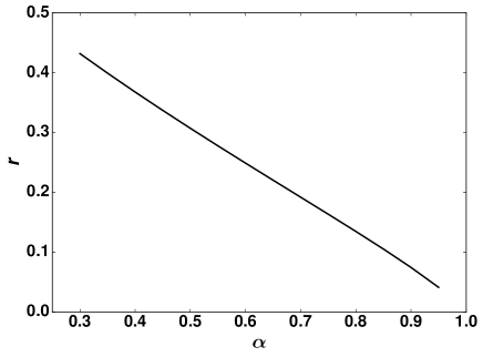
Figure 4: Critical ratio $r=(E_{M}/E_{J})_{C}$, as function of $\alpha$, at which the local maximum $T_{m}$ and minimum $T^{*}$ merge. Above, the resistance is a monotonous function of temperature, see also Fig. 5. The curve is close to be linear and well fitted by $(E_{M}/E_{J})_{C}=0.605-0.590\,\alpha$.

III.3 Non-perturbative resummation

We mentioned in the preceding section that perturbation theory fails at low temperature since $E_{M}$ multiplies a relevant operator. The description of the crossover to very low temperatures thus requires a resummation of the whole perturbation series, and such an exact resummation is not available for general $\alpha$ when both $E_{J}$ and $E_{M}$ are non-zero.For $\alpha=1/2$ however, a refermionization technique kane_fisher ; mora ; furusaki has been successfully applied to compute the crossover for the resistance when $E_{J}=0$. We extend it below to non-zero $E_{J}$ where an exact crossover can also be formulated.

The main idea is to interpret $\text{e}^{\,\text{i}\,e\hat{\phi}}\,$ as a bosonized form of a fermion operator $\hat{\psi}$. At zero temperature, with a chiral Hamiltonian

$$H_{0}=-\text{i}\,\displaystyle\int\hat{\psi}^{\dagger}(x)\,\partial_{x}\,\hat{\psi}(x)$$ (28)

the correlation function is

$$\left\langle\hat{\psi}^{\dagger}(x,t)\hat{\psi}(0,0)\right\rangle={\mathchoice{\dfrac{1}{2\pi\text{i}\,(t-x)}}{\dfrac{1}{2\pi\text{i}\,(t-x)}}{\frac{1}{2\pi\text{i}\,(t-x)}}{\frac{1}{2\pi\text{i}\,(t-x)}}}$$ (29)

At zero temperature and for $t\gg\tau_{s}=R{}_{\text{s}}C$, the integral (20) gives

$$\left\langle\text{e}^{\,\text{i}\,e\hat{\phi}(t,0)}\,\,\text{e}^{\,-\text{i}\,e\hat{\phi}(0,0)}\,\right\rangle\simeq\text{e}^{\,-\text{i}\,\pi/(4\alpha)}\,\times\left({\mathchoice{\dfrac{\tau_{s}}{\text{e}^{\,\gamma}\,\,t}}{\dfrac{\tau_{s}}{\text{e}^{\,\gamma}\,\,t}}{\frac{\tau_{s}}{\text{e}^{\,\gamma}\,\,t}}{\frac{\tau_{s}}{\text{e}^{\,\gamma}\,\,t}}}\right)^{1/(2\alpha)}$$ (30)

For $\alpha=1/2$, the correlator of $\text{e}^{\,\text{i}\,e\hat{\phi}}\,$ has the same time dependence as (29). The bosonization formula compatible with (30) and (29) is

$$\hat{\psi}(0)=\sqrt{{\mathchoice{\dfrac{\text{e}^{\,\gamma}\,}{\pi\tau{}_{\text{s}}}}{\dfrac{\text{e}^{\,\gamma}\,}{\pi\tau{}_{\text{s}}}}{\frac{\text{e}^{\,\gamma}\,}{\pi\tau{}_{\text{s}}}}{\frac{\text{e}^{\,\gamma}\,}{\pi\tau{}_{\text{s}}}}}}\,\hat{a}\,\text{e}^{\,\text{i}\,e\hat{\phi}(0)}\,$$ (31)

$\hat{a}$ is a local Majorana fermion with $\hat{a}=\hat{a}^{\dagger}$ and $\hat{a}^{2}=1/2$. $\hat{a}$ ensures the anticommutation rules for the fermionic field $\hat{\psi}(x)$. With the representation (31), the quadratic part of Eq.(14) can be remplaced by the Hamiltonian (28), and

$$-E_{M}\cos\Big{(}e\hat{\phi}(0)\Big{)}=-r_{M}\,\hat{a}\,\Big{(}\hat{\psi}(0)-\hat{\psi}^{\dagger}(0)\Big{)}\\ \text{with}\quad r_{M}=E_{M}\sqrt{{\mathchoice{\dfrac{\pi\tau{}_{\text{s}}}{\text{e}^{\,\gamma}\,}}{\dfrac{\pi\tau{}_{\text{s}}}{\text{e}^{\,\gamma}\,}}{\frac{\pi\tau{}_{\text{s}}}{\text{e}^{\,\gamma}\,}}{\frac{\pi\tau{}_{\text{s}}}{\text{e}^{\,\gamma}\,}}}}$$ (32)

A straightforward point-splitting calculation connects $\text{e}^{\,2\text{i}\,e\hat{\phi}(0)}\,$ to $\hat{\psi}(0)\,\partial_{x}\hat{\psi}(0)$, since $\hat{\psi}(0)\hat{\psi}(0)=0$ due to Fermi statistics. The two operators have scaling dimension $2$ when $\alpha=1/2$. The precise connection is obtained by identifying the two-point correlators using Eq.(29), with the result

$$-E_{J}\cos(2e\hat{\phi}(0))=\text{i}\,r_{J}\,\Big{(}\hat{\psi}(0)\,\partial_{x}\hat{\psi}(0)+\hat{\psi}^{\dagger}(0)\,\partial_{x}\hat{\psi}^{\dagger}(0)\Big{)}\\ \text{with}\quad r_{J}={\mathchoice{\dfrac{\pi\,{\tau{}_{\text{s}}}^{2}\,E_{J}}{\text{e}^{\,2\gamma}\,}}{\dfrac{\pi\,{\tau{}_{\text{s}}}^{2}\,E_{J}}{\text{e}^{\,2\gamma}\,}}{\frac{\pi\,{\tau{}_{\text{s}}}^{2}\,E_{J}}{\text{e}^{\,2\gamma}\,}}{\frac{\pi\,{\tau{}_{\text{s}}}^{2}\,E_{J}}{\text{e}^{\,2\gamma}\,}}}$$ (33)

The refermionized Hamiltonian takes the form

$$H=-\text{i}\,\displaystyle\int\hat{\psi}^{\dagger}(x)\,\partial_{x}\,\hat{\psi}(x)-r_{M}\,\hat{a}\,\Big{(}\hat{\psi}(0)-\hat{\psi}^{\dagger}(0)\Big{)}\\ +\text{i}\,r_{J}\,\Big{(}\hat{\psi}(0)\,\partial_{x}\hat{\psi}(0)+\hat{\psi}^{\dagger}(0)\,\partial_{x}\hat{\psi}^{\dagger}(0)\Big{)},$$ (34)

which is quadratic and exactly solvable. This effective Hamiltonian allows for a complete resummation for energies smaller than $E_{C}$. Interestingly, Eq.(34) already appeared in a different context lin ; fidkowski ; zuo ; pikulin ; sela as it can represent a semi-infinite helical wire - unfolded as a chiral mode on an infinite line - coupled at $x=0$ to a topological superconductor hosting a single Majorana bound state at its edge. $r_{M}$ plays the role of the tunnel coupling to the Majorana bound state while $r_{J}$ generates Andreev reflections at the superconductor. In this model, an incoming electron can be reflected as an electron or an hole (and vice versa).

Eq.(34) is easily diagonalized using a mode expansion fidkowski ; sela for $\hat{\psi}(x)$ and $\hat{\psi}^{\dagger}(x)$ summarized in Appendix C. Moreover, we can describe the relation between the left-moving electrons/holes $(x<0)$ and the right-moving electrons/holes $(x>0)$ with the S-matrix. At the formal level, the second term in the expression (16) of the resistance, involving the correlator $\langle\hat{f}(\tau)\hat{f}(0)\rangle$, coincides with the differential conductance of the boundary helical model fidkowski . Hence, the resistance (16) can be expressed using one of the S-matrix components:

$${\mathchoice{\dfrac{R}{R{}_{\text{s}}}}{\dfrac{R}{R{}_{\text{s}}}}{\frac{R}{R{}_{\text{s}}}}{\frac{R}{R{}_{\text{s}}}}}=1-\displaystyle\int_{-\infty}^{+\infty}\mathrm{d}\omega\,\bigg{(}-{\mathchoice{\dfrac{\partial n_{f}}{\partial\omega}}{\dfrac{\partial n_{f}}{\partial\omega}}{\frac{\partial n_{f}}{\partial\omega}}{\frac{\partial n_{f}}{\partial\omega}}}\bigg{)}\,|S{}_{\text{ph}}(\omega)|^{2}$$ (35)

where $n_{f}(\omega)=(1+e^{\beta\omega})^{-1}$ is the Fermi distribution and $S{}_{\text{ph}}$ is the probability for an incoming electron with energy $\omega$ to be reflected as a hole. The derivation of $S{}_{\text{ph}}$ is reproduced in Appendix C:

$$S{}_{\text{ph}}(\omega)={\mathchoice{\dfrac{\text{i}\,(2r_{J}\,\omega^{2}+{r_{M}}^{2})}{\text{i}\,{r_{M}}^{2}+\omega\,(1+r_{J}{r_{M}}^{2}+{r_{J}}^{2}\omega^{2})}}{\dfrac{\text{i}\,(2r_{J}\,\omega^{2}+{r_{M}}^{2})}{\text{i}\,{r_{M}}^{2}+\omega\,(1+r_{J}{r_{M}}^{2}+{r_{J}}^{2}\omega^{2})}}{\frac{\text{i}\,(2r_{J}\,\omega^{2}+{r_{M}}^{2})}{\text{i}\,{r_{M}}^{2}+\omega\,(1+r_{J}{r_{M}}^{2}+{r_{J}}^{2}\omega^{2})}}{\frac{\text{i}\,(2r_{J}\,\omega^{2}+{r_{M}}^{2})}{\text{i}\,{r_{M}}^{2}+\omega\,(1+r_{J}{r_{M}}^{2}+{r_{J}}^{2}\omega^{2})}}}$$ (36)

in agreement with Ref. fidkowski, . Inserting Eq.(36) into Eq. (35), the effective resistance reads

$${\mathchoice{\dfrac{R}{R{}_{\text{s}}}}{\dfrac{R}{R{}_{\text{s}}}}{\frac{R}{R{}_{\text{s}}}}{\frac{R}{R{}_{\text{s}}}}}=1-F\bigg{(}{\mathchoice{\dfrac{4\text{e}^{\,\gamma}\,}{\pi^{2}}}{\dfrac{4\text{e}^{\,\gamma}\,}{\pi^{2}}}{\frac{4\text{e}^{\,\gamma}\,}{\pi^{2}}}{\frac{4\text{e}^{\,\gamma}\,}{\pi^{2}}}}\,{\mathchoice{\dfrac{TE_{C}}{{E_{M}}^{2}}}{\dfrac{TE_{C}}{{E_{M}}^{2}}}{\frac{TE_{C}}{{E_{M}}^{2}}}{\frac{TE_{C}}{{E_{M}}^{2}}}},{\mathchoice{\dfrac{\pi^{5}}{8\text{e}^{\,3\gamma}\,}}{\dfrac{\pi^{5}}{8\text{e}^{\,3\gamma}\,}}{\frac{\pi^{5}}{8\text{e}^{\,3\gamma}\,}}{\frac{\pi^{5}}{8\text{e}^{\,3\gamma}\,}}}\,{\mathchoice{\dfrac{{E_{M}}^{2}E_{J}}{{E_{C}}^{3}}}{\dfrac{{E_{M}}^{2}E_{J}}{{E_{C}}^{3}}}{\frac{{E_{M}}^{2}E_{J}}{{E_{C}}^{3}}}{\frac{{E_{M}}^{2}E_{J}}{{E_{C}}^{3}}}}\bigg{)}$$ (37)

where the dimensionless function $F(\tilde{T},\tilde{r})$ is given by

$$F(\tilde{T},\tilde{r})=\displaystyle\int_{-\infty}^{+\infty}{\mathchoice{\dfrac{\mathrm{d}x}{2\operatorname{ch\,}^{2}x}}{\dfrac{\mathrm{d}x}{2\operatorname{ch\,}^{2}x}}{\frac{\mathrm{d}x}{2\operatorname{ch\,}^{2}x}}{\frac{\mathrm{d}x}{2\operatorname{ch\,}^{2}x}}}\,{\mathchoice{\dfrac{(2\tilde{T}^{2}\,\tilde{r}\,x^{2}+1)^{2}}{1+\tilde{T}^{2}x^{2}\,(1+\tilde{r}+\tilde{T}^{2}\,\tilde{r}^{2}x^{2})^{2}}}{\dfrac{(2\tilde{T}^{2}\,\tilde{r}\,x^{2}+1)^{2}}{1+\tilde{T}^{2}x^{2}\,(1+\tilde{r}+\tilde{T}^{2}\,\tilde{r}^{2}x^{2})^{2}}}{\frac{(2\tilde{T}^{2}\,\tilde{r}\,x^{2}+1)^{2}}{1+\tilde{T}^{2}x^{2}\,(1+\tilde{r}+\tilde{T}^{2}\,\tilde{r}^{2}x^{2})^{2}}}{\frac{(2\tilde{T}^{2}\,\tilde{r}\,x^{2}+1)^{2}}{1+\tilde{T}^{2}x^{2}\,(1+\tilde{r}+\tilde{T}^{2}\,\tilde{r}^{2}x^{2})^{2}}}}$$ (38)

For $E_{J}=0$ , the integration can be performed and we recover the known result shon_zaikin ; weiss_wollensak

$${\mathchoice{\dfrac{R}{R{}_{\text{s}}}}{\dfrac{R}{R{}_{\text{s}}}}{\frac{R}{R{}_{\text{s}}}}{\frac{R}{R{}_{\text{s}}}}}\bigg{|}_{E_{J}=0}=1-{\mathchoice{\dfrac{\pi{E_{M}}^{2}}{4\text{e}^{\,\gamma}\,E_{C}\,T}}{\dfrac{\pi{E_{M}}^{2}}{4\text{e}^{\,\gamma}\,E_{C}\,T}}{\frac{\pi{E_{M}}^{2}}{4\text{e}^{\,\gamma}\,E_{C}\,T}}{\frac{\pi{E_{M}}^{2}}{4\text{e}^{\,\gamma}\,E_{C}\,T}}}\,\Psi^{\prime}\bigg{(}{\mathchoice{\dfrac{1}{2}}{\dfrac{1}{2}}{\frac{1}{2}}{\frac{1}{2}}}+{\mathchoice{\dfrac{\pi{E_{M}}^{2}}{4\text{e}^{\,\gamma}\,E_{C}\,T}}{\dfrac{\pi{E_{M}}^{2}}{4\text{e}^{\,\gamma}\,E_{C}\,T}}{\frac{\pi{E_{M}}^{2}}{4\text{e}^{\,\gamma}\,E_{C}\,T}}{\frac{\pi{E_{M}}^{2}}{4\text{e}^{\,\gamma}\,E_{C}\,T}}}\bigg{)}$$ (39)

At zero temperature, one obtains $F=1$ consistent with a fully coherent Josephson junction. Let us emphasize that the result (37) was obtained assuming $T\ll 2E_{C}/\pi$ and $E_{J},E_{M}\ll E_{C}$. As a consequence, we have ${E_{M}}^{2}E_{J}/{E_{C}}^{3}\ll 1$ such that second parameter $\tilde{r}$ in Eq.(38) is always much smaller than one. At low temperature $T\ll{E_{M}}^{2}/E_{C}$, we can therefore ignore $E_{J}$ to obtain the asymptotic expression

$${\mathchoice{\dfrac{R(T)}{R{}_{\text{s}}}}{\dfrac{R(T)}{R{}_{\text{s}}}}{\frac{R(T)}{R{}_{\text{s}}}}{\frac{R(T)}{R{}_{\text{s}}}}}\simeq{\mathchoice{\dfrac{4\text{e}^{\,2\gamma}\,}{3\pi^{2}}}{\dfrac{4\text{e}^{\,2\gamma}\,}{3\pi^{2}}}{\frac{4\text{e}^{\,2\gamma}\,}{3\pi^{2}}}{\frac{4\text{e}^{\,2\gamma}\,}{3\pi^{2}}}}\,\left({\mathchoice{\dfrac{T}{{E_{M}}^{2}/E_{C}}}{\dfrac{T}{{E_{M}}^{2}/E_{C}}}{\frac{T}{{E_{M}}^{2}/E_{C}}}{\frac{T}{{E_{M}}^{2}/E_{C}}}}\right)^{2}.$$ (40)

In the opposite limit $T\gg{E_{M}}^{2}/E_{C}$, we keep $\tilde{r}\sim E_{J}$ and recover the result Eq. (24) of the preceding section for $\alpha=1/2$.

We plot in Fig. 5 the interpolation between Eq. (37) and Eq. (22) for different values of ($E_{M}/E_{C},E_{J}/E_{C})$. We thus observe the crossover where the two extrema disappear.

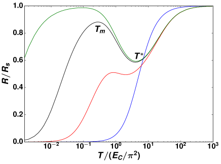
Figure 5: Dimensionless resistance $R/R{}_{\text{s}}$ as function of the reduced temperature $T/(E_{C}/\pi^{2})$ for $\alpha=1/2$ and different values of $(E_{J}/E_{C},E_{M}/E_{C})$ obtained by interpolation between Eq. (37) and Eq. (22). We represent $(E_{J}/E_{C},E_{M}/E_{C})=(0.8,0.1)$ (red line), $(0.03,0.5)$ (blue line), $(0.8,0.006)$ (green line), $(0.8,0.03)$ (black line). The two extrema $T_{m}$ and $T^{*}$ merge at $E_{J}/E_{M}=0.31$, see Fig. 4.

IV Large Josephson energy

The analysis of Sec. III was restricted to the Coulomb blockade regime where the bare charging energy $E_{C}$ is the largest energy scale. Coulomb blockade tends to pin the superconductor charge which has the effect of delocalizing the conjugated phase variable. The shunted Josephson junction is then closer to an insulator, with a differential resistance below but in the vicinity of $R_{s}$, except at very low temperature where the relevant Josephson energy $E_{M}$ takes over and reestablishes a dissipationless Josephson tunneling.

The resulting resistance, shown in Fig. 5, exhibits a local minimum at $T=T^{*}\sim E_{C}$ with a distance to the fully shunted junction $R=R_{s}$ increasing with $E_{J}$, reflecting a partial relocalization of the phase. This scaling suggests that the local minimum keeps decreasing with $E_{J}/E_{C}$ until it reaches an almost vanishing resistance in a certain temperature range for $E_{J}$ larger than $E_{C}$. In what follows, we consider directly the regime of deep potential wells $E_{J}\gg E_{C}$ while $E_{M}$ is chosen below the plasma frequency $\omega{}_{\text{p}}=\sqrt{8E_{J}E_{C}}$.

We first diagonalize the model in the absence of the ohmic environment in Sec. IV.1 and then take in Sec. IV.2 $\alpha=1/2$ where a mapping to the Emery-Kivelson model can be demonstrated. This gives the exact resistance for $\alpha=1/2$ and a qualitative picture for $\alpha$ between $1/4$ and $1$, extending the analysis of Sec. III.

IV.1 Dissipationless case

In the absence of dissipation, the Hamiltonian (1) simplifies as $H=H_{0}-E_{M}\cos(\hat{\varphi}/2)$ with the transmon Hamiltonian koch

$$H_{0}(n_{g})=4E_{C}\,(\hat{N}-n_{g})^{2}-E_{J}\cos\hat{\varphi}$$ (41)

where $n_{g}$ is the offset charge of the capacitor. In the phase representation, $\hat{N}=i\partial_{\varphi}$ is acting on $2\pi$-periodic functions, and $H_{0}$ can be diagonalized exactly using Mathieu functions wilkinson . For $E_{J}\gg E_{C}$, the energy of the ground state takes the suggestive form

$$E_{0}(n_{g})={\mathchoice{\dfrac{\omega{}_{\text{p}}}{2}}{\dfrac{\omega{}_{\text{p}}}{2}}{\frac{\omega{}_{\text{p}}}{2}}{\frac{\omega{}_{\text{p}}}{2}}}-t_{0}\cos\left(2\pi n_{g}\right),$$ (42)

where koch

$$t_{0}=16\,\sqrt{\frac{E_{J}E_{C}}{\pi}}\,\left(\frac{E_{J}}{2E_{C}}\right)^{1/4}\exp\left(-\sqrt{\frac{8E_{J}}{E_{C}}}\right)$$ (43)

The ground state energy has a periodicity of one in $n_{g}$ as expected from the discreteness of $\hat{N}$.

Although the above derivation is self-contained, it is instructive to formulate it using a Bloch band description shon_zaikin ; catelani . The Hamiltonian $H_{0}$ (41) with the compact phase $\hat{\varphi}$ in $[0,2\pi]$ is mathematically equivalent to solving $H_{0}(0)$ with an extended phase, i.e. $\hat{\varphi}$ between $-\infty$ and $\infty$, with $n_{g}$ playing the role of the quasimomentum. In this langage, Eq. (42) as function of $n_{g}$ is a band dispersion. Focussing again on the regime $E_{J}\gg E_{C}$, the wavefunctions of low-energy eigenstates are strongly localized near the minima of the cosine potential and the Wannier function of the lowest band is the ground state of an harmonic oscillator,

$$W_{0}(\varphi)=\left(\frac{E_{J}}{8\pi^{2}E_{C}}\right)^{1/8}\,\exp\left(-\frac{\varphi^{2}}{2}\sqrt{\frac{E_{J}}{8E_{C}}}\right),$$ (44)

with energy $\omega{}_{\text{p}}$. The small overlap between consecutive Wannier functions induces a nearest-neighbor hopping term $t_{0}/2$. We thus obtain a tight-binding model whose diagonalization reproduces Eq. (42) and $t_{0}$ is identified as the bandwidth of the lowest band in the cosine potential.

Next, we include $E_{M}$ and numerically evaluate the spectrum of $H$. The presence of $E_{M}$ doubles the size of the unit cell folding the spectrum at $n_{g}=\pm 1/2$, corresponding to single-electron tunneling, and opening gaps at the edge of the new Brillouin zone as illustrated in Fig.6. In order to make further analytical progress, we consider $E_{M}<\omega{}_{\text{p}}$ such that the different bands of $H_{0}$ are not mixed, and project the Hamiltonian onto the lowest band. Due to non-zero $E_{M}$, the wavefunctions must have a periodicity of $4\pi$ in $\varphi$. For a given charge offset $n_{g}$, we find two such functions in the lowest band yavilberg ; ginossar :

$$\Psi_{\pm,n_{g}}(\varphi)=\sum_{p\in\mathbb{Z}}(\pm 1)^{p}\,W_{0}(\varphi-2p\pi)e^{in_{g}(2p\pi-\varphi)}$$ (45)

with energies $E_{0}(n_{g})$ and $E_{0}(n_{g}+1/2)$. These are $4\pi$-periodic functions, even and odd with respect to the parity operator $(-1)^{\hat{N}}\Psi_{\pm,n_{g}}=\pm\Psi_{\pm,n_{g}}$. After projecting the Hamiltonian $H$ onto the basis (45), we get

$$\begin{split}H_{LE}(n_{g})&=t_{0}\cos\left(2\pi n_{g}\right)\sigma_{z}+c_{0}E_{M}\sigma_{x}\\ &+d_{0}E_{M}\sigma_{y}\sin\left(2\pi n_{g}\right),\end{split}$$ (46)

where $\sigma_{i}$ ($i=x,y,z$) are Pauli matrices operating in parity space and the constant term $\omega{}_{\text{p}}/2$ has been removed. This derivation of the different overlaps in Eq. (46) uses that $W_{0}(\varphi)$ takes appreciable values only close to $\varphi\simeq 0$. One consequence is that $E_{M}$ does not enter the diagonal elements - or only with a very small contribution neglected here, whereas there is a perfect overlap $c_{0}=1$ along $\sigma_{x}$. The overlap along $\sigma_{y}$ is given by

$$d_{0}=\frac{2^{1/3}t_{0}}{3^{-1/3}\omega_{p}}\,\sqrt{\frac{E_{C}}{E_{J}}}\,\Gamma\left({\mathchoice{\dfrac{2}{3}}{\dfrac{2}{3}}{\frac{2}{3}}{\frac{2}{3}}}\right)\ll 1,$$ (47)

and can be also neglected. The $\sigma_{x}$ and $\sigma_{y}$ components in Eq. (46) can be seen respectively as a staggered potential and a staggered hopping amplitude in the tight-binding model. We note that applying a non-zero flux between the two Josephson junctions can change the relative values of $c_{0}$ and $d_{0}$. The limiting case $c_{0}=0$ and $d_{0}=1$ corresponds to the SSH model ssh .

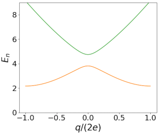
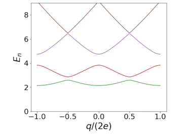
Figure 6: Lowest bands obtained by a numerical solution of $H$ as a function of the charge offset $n_{g}$ in the absence of dissipation. The numerical solution is found qutip1 ; qutip2 by performing a truncation in the charge basis $|n\rangle$ (eigenstates of $\hat{N}$) and diagonalizing a finite-size version of $H$. In both pictures, $E_{C}=1$ and $E_{J}=3$. (a) Spectrum for $E_{M}=0$. (b) Spectrum for $E_{M}=3$. Gaps open at the edges of the reduced Brillouin zone.

IV.2 Effective Hamiltonian with dissipation

The projection to the lowest band of the extended potential can still be applied to the original Hamiltonian (1) provided the ohmic dissipation is not too strong. It amounts to an adiabatic approximation where one replaces the charge offset by $2en_{g}=-\hat{Q}-\int^{t}\mathrm{d}t^{\prime}\,I_{0}(t^{\prime})$ in the transmon Hamiltonian $H_{0}$ (41). It is justified as long the input current $I_{0}$ is weak and varies slowly in time, and if $\alpha^{2}\ll 2\pi^{2}E_{J}/E_{C}$ korshunov .

The projected Hamiltonian is

$$H_{P}=H_{LE}\left({\mathchoice{\dfrac{\hat{Q}}{2e}}{\dfrac{\hat{Q}}{2e}}{\frac{\hat{Q}}{2e}}{\frac{\hat{Q}}{2e}}}+{\mathchoice{\dfrac{Q_{0}(t)}{2e}}{\dfrac{Q_{0}(t)}{2e}}{\frac{Q_{0}(t)}{2e}}{\frac{Q_{0}(t)}{2e}}}\right)+H_{R{}_{\text{s}}},$$ (48)

where $Q_{0}(t)=\int^{t}\mathrm{d}t^{\prime}\,I_{0}(t^{\prime})$, which we expand to first order in $Q_{0}$ as

$$H_{P}\simeq H_{LE}\left({\mathchoice{\dfrac{\hat{Q}}{2e}}{\dfrac{\hat{Q}}{2e}}{\frac{\hat{Q}}{2e}}{\frac{\hat{Q}}{2e}}}\right)+H_{R{}_{\text{s}}}-t_{0}\frac{\pi Q_{0}(t)}{e}\sin\left({\mathchoice{\dfrac{\pi\hat{Q}}{e}}{\dfrac{\pi\hat{Q}}{e}}{\frac{\pi\hat{Q}}{e}}{\frac{\pi\hat{Q}}{e}}}\right),$$ (49)

and, for $Q_{0}=0$,

$$H_{P}=t_{0}\cos\Big{(}{\mathchoice{\dfrac{\pi}{e}}{\dfrac{\pi}{e}}{\frac{\pi}{e}}{\frac{\pi}{e}}}\hat{Q}\Big{)}\,\sigma_{z}+E_{M}\,\sigma_{x}+H_{R{}_{\text{s}}}$$ (50)

Due to the absence of the capacitive term, the mode expansion of the fields in the transmission line differs slightly from Sec. II.2 and we have

$$\hat{\phi}(0) =\sqrt{{\mathchoice{\dfrac{R{}_{\text{s}}}{4\pi}}{\dfrac{R{}_{\text{s}}}{4\pi}}{\frac{R{}_{\text{s}}}{4\pi}}{\frac{R{}_{\text{s}}}{4\pi}}}}\,\displaystyle\int_{0}^{\omega{}_{\text{p}}}{\mathchoice{\dfrac{\mathrm{d}\omega}{\sqrt{\omega}}}{\dfrac{\mathrm{d}\omega}{\sqrt{\omega}}}{\frac{\mathrm{d}\omega}{\sqrt{\omega}}}{\frac{\mathrm{d}\omega}{\sqrt{\omega}}}}\,\bigg{[}{\mathchoice{\dfrac{2}{1-\text{i}\,\tau_{0}\omega}}{\dfrac{2}{1-\text{i}\,\tau_{0}\omega}}{\frac{2}{1-\text{i}\,\tau_{0}\omega}}{\frac{2}{1-\text{i}\,\tau_{0}\omega}}}\,a{}_{\text{in,$\omega$}}+\text{h.c}\bigg{]},$$ (51a)

$$\hat{Q} =\frac{1}{\sqrt{4\pi R{}_{\text{s}}}}\int_{0}^{\omega{}_{\text{p}}}{\mathchoice{\dfrac{d\omega}{\sqrt{\omega}}}{\dfrac{d\omega}{\sqrt{\omega}}}{\frac{d\omega}{\sqrt{\omega}}}{\frac{d\omega}{\sqrt{\omega}}}}\left[{\mathchoice{\dfrac{-2i\tau_{0}\omega}{1-\text{i}\,\tau_{0}\omega}}{\dfrac{-2i\tau_{0}\omega}{1-\text{i}\,\tau_{0}\omega}}{\frac{-2i\tau_{0}\omega}{1-\text{i}\,\tau_{0}\omega}}{\frac{-2i\tau_{0}\omega}{1-\text{i}\,\tau_{0}\omega}}}a_{\rm in,\omega}-{\rm h.c.}\right],$$ (51b)

where $\tau_{0}$ is a regularizing time that is eventually sent to infinity. Frequencies are cut off at the plasma frequency $\omega{}_{\text{p}}$ at which higher bands start to play a role. The correlator $K_{\hat{Q}}(t)=\langle\text{e}^{\,i\pi\hat{Q}(t)/e}\,\text{e}^{\,-i\pi\hat{Q}(0)/e}\,\rangle$ describes now charge fluctuations. At zero temperature, one gets

$$K_{\hat{Q}}(t)=\exp\left[2\alpha\int_{0}^{\omega{}_{\text{p}}}{\mathchoice{\dfrac{d\omega}{\omega}}{\dfrac{d\omega}{\omega}}{\frac{d\omega}{\omega}}{\frac{d\omega}{\omega}}}{\mathchoice{\dfrac{(\tau_{0}\omega)^{2}}{1+(\tau_{0}\omega)^{2}}}{\dfrac{(\tau_{0}\omega)^{2}}{1+(\tau_{0}\omega)^{2}}}{\frac{(\tau_{0}\omega)^{2}}{1+(\tau_{0}\omega)^{2}}}{\frac{(\tau_{0}\omega)^{2}}{1+(\tau_{0}\omega)^{2}}}}\left(e^{-i\omega t}-1\right)\right],$$ (52)

or, for $1/\omega{}_{\text{p}}\ll t\ll\tau_{0}$ and $\alpha$, $K_{\hat{Q}}(t)\sim 1/(\omega{}_{\text{p}}t)$. The same fermionization as Eq. (31) can be performed such that

$$t_{0}\,\cos\Big{(}{\mathchoice{\dfrac{\pi}{e}}{\dfrac{\pi}{e}}{\frac{\pi}{e}}{\frac{\pi}{e}}}\,\hat{Q}\Big{)}=r_{0}\,\hat{a}\,\Big{(}\hat{\psi}(0)-\hat{\psi}^{\dagger}(0)\Big{)}$$ (53)

with $r_{0}\sim t_{0}/\sqrt{\omega{}_{\text{p}}}$. The Hamiltonian (50) can be further transformed using the representation of Pauli matrices in terms of Majorana fermions pauli , i.e $\sigma_{x}=\text{i}\,\eta_{2}\eta_{3}$, $\sigma_{y}=\text{i}\,\eta_{3}\eta_{1}$ and $\sigma_{z}=\text{i}\,\eta_{1}\eta_{2}$. The commutation relations of the Pauli matrices are ensured by the Clifford algebra $\{\eta_{i},\eta_{j}\}=2\delta_{ij}$. Using these representations, the Hamiltonian (50) becomes

$$H_{P}=-\text{i}\,\displaystyle\int\psi^{\dagger}(x)\partial_{x}\psi+\text{i}\,E_{M}\,\eta_{2}\eta_{3}\\ -\text{i}\,r_{0}\,\Big{(}\hat{\psi}(0)-\hat{\psi}^{\dagger}(0)\Big{)}\,\hat{a}\,\eta_{1}\eta_{2}.$$ (54)

$\hat{a}\,\eta_{1}$ commutes with $H_{P}$ such that we can choose $\hat{a}\,\eta_{1}=\text{i}\,/\sqrt{2}$ and,

$$H_{P}=-\text{i}\,\displaystyle\int\psi^{\dagger}(x)\partial_{x}\psi+\text{i}\,E_{M}\,\eta_{2}\eta_{3}\\ +{\mathchoice{\dfrac{r_{0}}{\sqrt{2}}}{\dfrac{r_{0}}{\sqrt{2}}}{\frac{r_{0}}{\sqrt{2}}}{\frac{r_{0}}{\sqrt{2}}}}\Big{(}\hat{\psi}(0)-\hat{\psi}^{\dagger}(0)\Big{)}\,\eta_{2}.$$ (55)

This Hamiltonian coincides exactly with the effective model found by Emery and Kivelson emer-kivel ; georges to solve the two-channel Kondo model in the presence of a magnetic field. $r_{0}$ is a relevant operator driving the system to a strong-coupling fixed point where $r_{0}$ is large - or $E_{J}$ large - and the Majorana fermion $\eta_{2}$ is screened. The effect of the magnetic field $\sim E_{M}$ is to stop the renormalization group flow. Eq. (55) is quadratic and therefore analytically solvable.

IV.3 Resistance

The voltage drop across the junction is

$$\begin{split}V&=\langle\dot{\hat{\phi}}(t)\rangle=\text{i}\,\langle[H_{P},\hat{\phi}]\rangle\\[5.69054pt] &=-t_{0}{\mathchoice{\dfrac{\pi}{e}}{\dfrac{\pi}{e}}{\frac{\pi}{e}}{\frac{\pi}{e}}}\langle\sin\Big{(}{\mathchoice{\dfrac{\pi}{e}}{\dfrac{\pi}{e}}{\frac{\pi}{e}}{\frac{\pi}{e}}}\hat{Q}\Big{)}\,\sigma_{z}\rangle+\text{i}\,\langle[H_{R{}_{\text{s}}},\hat{\phi}]\rangle\end{split}$$ (56)

where we use again the notation $\hat{\phi}(t)=\hat{\phi}(x=0,t)$. The second term $[H_{R{}_{\text{s}}},\hat{\phi}]$ gives zero. Using the Kubo formula and Eq. (49) for the linear coupling to the bias current, we obtain the expression for the resistance

$${\mathchoice{\dfrac{R(T)}{R{}_{\text{s}}}}{\dfrac{R(T)}{R{}_{\text{s}}}}{\frac{R(T)}{R{}_{\text{s}}}}{\frac{R(T)}{R{}_{\text{s}}}}}=2\pi\,\alpha\,\lim\limits_{\omega\to 0}\,\mathcal{R}\Big{(}{\mathchoice{\dfrac{\text{i}\,}{\omega}}{\dfrac{\text{i}\,}{\omega}}{\frac{\text{i}\,}{\omega}}{\frac{\text{i}\,}{\omega}}}\,\lim\limits_{\text{i}\,\omega_{n}\to\omega+\text{i}\,0^{+}}\,\displaystyle\int_{0}^{\beta}\,\text{e}^{\,\text{i}\,\omega_{n}\tau}\,\langle\hat{g}(\tau)\hat{g}(0)\rangle\Big{)}$$ (57)

where

$$\hat{g}(\tau)=\text{i}\,t_{0}\,\sin\Big{(}{\mathchoice{\dfrac{\pi}{e}}{\dfrac{\pi}{e}}{\frac{\pi}{e}}{\frac{\pi}{e}}}\,\hat{Q}(\tau)\Big{)}\,\eta_{1}(\tau)\,\eta_{2}(\tau)\\[5.69054pt] =-\text{i}\,{\mathchoice{\dfrac{r_{0}}{\sqrt{2}}}{\dfrac{r_{0}}{\sqrt{2}}}{\frac{r_{0}}{\sqrt{2}}}{\frac{r_{0}}{\sqrt{2}}}}\,\Big{(}\hat{\psi}(\tau)+\hat{\psi}^{\dagger}(\tau)\Big{)}\,\eta_{2}(\tau)$$ (58)

where $\hat{\psi}(\tau)=\hat{\psi}(\tau,x=0)$. Using the S-matrix formalism introduced in the previous section with Eq.(54), we finally obtain

$${\mathchoice{\dfrac{R(T)}{R{}_{\text{s}}}}{\dfrac{R(T)}{R{}_{\text{s}}}}{\frac{R(T)}{R{}_{\text{s}}}}{\frac{R(T)}{R{}_{\text{s}}}}}=\displaystyle\int_{-\infty}^{+\infty}\mathrm{d}\omega\,\bigg{(}-{\mathchoice{\dfrac{\partial n_{f}}{\partial\omega}}{\dfrac{\partial n_{f}}{\partial\omega}}{\frac{\partial n_{f}}{\partial\omega}}{\frac{\partial n_{f}}{\partial\omega}}}\bigg{)}{\mathchoice{\dfrac{{r_{0}}^{4}\,\omega^{2}}{(\omega^{2}-4{E_{M}}^{2})^{2}+{r_{0}}^{4}\,\omega^{2}}}{\dfrac{{r_{0}}^{4}\,\omega^{2}}{(\omega^{2}-4{E_{M}}^{2})^{2}+{r_{0}}^{4}\,\omega^{2}}}{\frac{{r_{0}}^{4}\,\omega^{2}}{(\omega^{2}-4{E_{M}}^{2})^{2}+{r_{0}}^{4}\,\omega^{2}}}{\frac{{r_{0}}^{4}\,\omega^{2}}{(\omega^{2}-4{E_{M}}^{2})^{2}+{r_{0}}^{4}\,\omega^{2}}}}$$ (59)

For $E_{M}=0$, one obtains weiss_wollensak

$${\mathchoice{\dfrac{R}{R{}_{\text{s}}}}{\dfrac{R}{R{}_{\text{s}}}}{\frac{R}{R{}_{\text{s}}}}{\frac{R}{R{}_{\text{s}}}}}={\mathchoice{\dfrac{{r_{0}}^{2}}{2\pi T}}{\dfrac{{r_{0}}^{2}}{2\pi T}}{\frac{{r_{0}}^{2}}{2\pi T}}{\frac{{r_{0}}^{2}}{2\pi T}}}\,\Psi^{\prime}\Big{(}{\mathchoice{\dfrac{1}{2}}{\dfrac{1}{2}}{\frac{1}{2}}{\frac{1}{2}}}+{\mathchoice{\dfrac{{r_{0}}^{2}}{2\pi T}}{\dfrac{{r_{0}}^{2}}{2\pi T}}{\frac{{r_{0}}^{2}}{2\pi T}}{\frac{{r_{0}}^{2}}{2\pi T}}}\Big{)}$$ (60)

with the infrared insulating fixed point, $R=R_{s}$, at zero temperature.

A non-zero $E_{M}$ drastically changes to the infrared superconducting fixed point. Eq. (59) gives the resistance $R=0$ at zero temperature. The temperature dependence of the resistance is shown in Fig.7 by evaluating the integral in Eq. (59). For $T\gg E_{M}$, the integral simplifies as

$${\mathchoice{\dfrac{R}{R{}_{\text{s}}}}{\dfrac{R}{R{}_{\text{s}}}}{\frac{R}{R{}_{\text{s}}}}{\frac{R}{R{}_{\text{s}}}}}\simeq{\mathchoice{\dfrac{\pi}{4}}{\dfrac{\pi}{4}}{\frac{\pi}{4}}{\frac{\pi}{4}}}\,{\mathchoice{\dfrac{{r_{0}}^{2}}{T}}{\dfrac{{r_{0}}^{2}}{T}}{\frac{{r_{0}}^{2}}{T}}{\frac{{r_{0}}^{2}}{T}}}$$ (61)

We obtain the same expression as Eq. (60) in the high-temperature limit: for $T\gg E_{M}$, the resistance is only controlled by ${r_{0}}^{2}$.

The approach discussed in this section is limited to temperatures below the plasma frequency $\omega{}_{\text{p}}$. Above $\omega{}_{\text{p}}$, the phase delocalizes via thermal activation across the minima of the deep Josephson potential nozieres , and the resistance increases again until it reaches the insulating regime $R=R_{s}$ for temperature much larger than $E_{J}$.

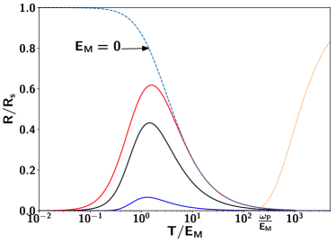
Figure 7: Resistance versus temperature for ${r_{0}}^{2}/2E_{M}=0.1$ (blue), $1$ (black), $2$ (red), where ${r_{0}}^{2}/E_{M}\sim{t_{0}}^{2}/\omega_{p}E_{M}$. The limiting case of vanishing $E_{M}$ is shown in dotted line for comparison. The analysis in this work is limited to temperatures lower than the plasma frequency $\omega_{p}$. Above, a thermally actived behaviour $\sim e^{-E_{J}/T}$ towards a full resistance $R=R_{s}$ occurs nozieres (dotted yellow line) corresponding to a complete delocalization of the phase.

V Conclusion

In this paper, we have considered a superconducting junction with a Josephson energy being the sum of two contributions: the usual $2\pi$-periodic energy and an additional $4\pi$-periodic energy which can be the sign of a topological junction hosting Majorana bound states. The model accounts for a single junction with the two periodicities or, alternatively, two separated Josephson junctions in parallel. The existence of the two commensurate phase periodicities is not necessarily a sign of topology but could also occur with, for instance, a Kondo impurity, a Josephson rhombus device or in hybrid ferromagnetic-superconducing junctions.

A sufficiently strong shunt resistor in parallel with the junction drives the device via a quantum phase transition to an insulating regime where the zero-temperature Josephson current is suppressed. We have focussed on values of the resistance such that the $2\pi$-periodic term alone would give an insulating state while the $4\pi$-periodic energy is still superconducting, resulting in a competition between the two terms. We have derived the corresponding non-monotonic behaviour of the total differential resistance of the device as a function of temperature.

For a charging energy much larger than the Josephson energy, the junction is essentially resistive at high temperature. The resistance increases with temperature for $T>E_{C}$ but decreases for $T<E_{C}$, reaching a minimum at $T=T^{*}\sim E_{C}$. For even lower temperatures, a crossover towards a fully superconducting junction with zero resistance was established below a local temperature maximum $T_{m}$. These features were first derived using perturbation theory and then an exact analytically expression was obtained when $\alpha=1/2$, or $R_{s}=2R{}_{\text{q}}$. The exact refermionization maps the model onto an helical one-dimensional wire coupled to a topological superconductor.

When the charging energy is the smallest energy scale, we confirmed the non-monotonic behaviour with a tight-binding approach connecting the Josephson wells. Delocalizing the superconducting phase, the hopping between the wells is suppressed by dissipation - by duality, the coupling of the phase to dissipation decreases with the shunt resistance - and a superconducting behaviour is restored at low energy. For $\alpha=1/2$, or $R_{s}=2R{}_{\text{q}}$, we find a mapping to the Emery-Kivelson line of the two-channel Kondo model under finite magnetic field. It provides again an exact expression for the temperature-dependent differential resistance.

A straightforward extension of our work is the study of the non-linear current-voltage characteristic where the weight of the Josephson peak is transferred by the environment to higher voltages didier . Also our analysis is restricted to an equilibrium electromagnetic environment torre2012 and the prospect of exciting photons around the Josephson junction mendes2015 offers an appealing direction of research.

Appendix A Linear response theory

We set $E_{M}=0$ to simplify the discussion but without loss of generality. The contribution $-I_{0}(t)\,\hat{\phi}(0)$ in the Hamiltonian (14) can be regarded as a perturbation. We use the framework of linear response theory to compute the voltage drop across the junction. The Kubo formula gives

$$V(t)=\left\langle\dot{\hat{\phi}}\right\rangle=\text{i}\,\,\displaystyle\int_{-\infty}^{t}\,\mathrm{d}t^{\prime}\,\left\langle\big{[}\dot{\hat{\phi}}(t),\hat{\phi}(t^{\prime})\big{]}\right\rangle\,I_{0}(t^{\prime})\\ =-\displaystyle\int_{-\infty}^{+\infty}\mathrm{d}t^{\prime}\,G_{\dot{\phi},\phi}^{\text{ret}}(t-t^{\prime})\,I_{0}(t^{\prime})$$ (62)

where $\hat{\phi}(t)=\hat{\phi}(x=0,t)$ and the retarded Green’s function

$$G^{\text{ret}}(t-t^{\prime})=-\text{i}\,\theta(t)\left\langle\big{[}\dot{\hat{\phi}}(t),\hat{\phi}(t^{\prime})\big{]}\right\rangle$$ (63)

where $\theta(t)$ is the Heaviside function. In Fourier space, Eq.(62) becomes $V(\omega)=-G^{\text{ret}}_{\dot{{\phi}},{\phi}}(\omega)\,I_{0}(\omega)$. $G^{\text{ret}}(\omega)$ is analytical in the upper complexe semiplane only. As a consequence, for a real argument $\omega$, the limit $\omega+\text{i}\,0^{+}$ has to be considered. Now, we use the notation $\phi_{0}=2e\,\hat{\phi}(0)$. With $G_{\dot{\phi},\phi}^{\text{ret}}(\omega)=-\text{i}\,\omega\,G_{{\phi},\phi}^{\text{ret}}(\omega)$, the linear resistance is

$$R(\omega)=R{}_{\text{s}}\,{\mathchoice{\dfrac{\alpha}{2\pi}}{\dfrac{\alpha}{2\pi}}{\frac{\alpha}{2\pi}}{\frac{\alpha}{2\pi}}}\times\text{i}\,\omega\,G_{{\phi_{0}},\phi_{0}}^{\text{ret}}(\omega+\text{i}\,0^{+})$$ (64)

In the last expression, we have used $1/4e^{2}=R{}_{\text{s}}\,\alpha/2\pi$. To compute $G^{\text{ret}}(\omega+\text{i}\,0^{+})$, we compute another correlation function in the imaginary time formalism and do an analytic continuation. We can compute the Matsubara Green’s function $G(\tau)=-\left\langle\mathcal{T}_{\tau}{\phi_{0}}(\tau){\phi}_{0}(0)\right\rangle$ where $\mathcal{T}_{\tau}$ is the time-ordering. In this article, we want to compute the DC resistance ($\omega\to 0$) so we need to take the real part of Eq.(64). The linear resistance becomes

$${\mathchoice{\dfrac{R(T)}{R{}_{\text{s}}}}{\dfrac{R(T)}{R{}_{\text{s}}}}{\frac{R(T)}{R{}_{\text{s}}}}{\frac{R(T)}{R{}_{\text{s}}}}}=-{\mathchoice{\dfrac{\alpha}{2\pi}}{\dfrac{\alpha}{2\pi}}{\frac{\alpha}{2\pi}}{\frac{\alpha}{2\pi}}}\,\lim\limits_{\omega\to 0}\mathcal{R}\bigg{[}\text{i}\,\omega\times\\ \lim\limits_{\text{i}\,\omega_{n}\to\omega+\text{i}\,0^{+}}\,\displaystyle\int_{0}^{\beta}\mathrm{d}\tau\,\text{e}^{\,\text{i}\,\omega_{n}\tau}\,\,\left\langle{\phi_{0}}(\tau){\phi}_{0}(0)\right\rangle\bigg{]}$$ (65)

In the last expression the time-ordering factor doesn’t appear because the $\tau$ is between $0$ and $\beta>0$. We can use an other expression of (65) where the correlator is written with matsubara frequencies:

$${\mathchoice{\dfrac{R(T)}{R{}_{\text{s}}}}{\dfrac{R(T)}{R{}_{\text{s}}}}{\frac{R(T)}{R{}_{\text{s}}}}{\frac{R(T)}{R{}_{\text{s}}}}}=-{\mathchoice{\dfrac{\alpha}{2\pi}}{\dfrac{\alpha}{2\pi}}{\frac{\alpha}{2\pi}}{\frac{\alpha}{2\pi}}}\,\lim\limits_{\omega\to 0}\mathcal{R}\bigg{[}\text{i}\,\omega\,\lim\limits_{\text{i}\,\omega_{n}\to\omega+\text{i}\,0^{+}}\,{\mathchoice{\dfrac{1}{\beta}}{\dfrac{1}{\beta}}{\frac{1}{\beta}}{\frac{1}{\beta}}}\,{\displaystyle\sum\limits_{\text{i}\,\omega_{k}}}\,\left\langle{\phi}_{0}(\text{i}\,\omega_{n}){\phi}_{0}(\text{i}\,\omega_{k})\right\rangle\bigg{]}$$ (66)

The analytical expression of the linear resistance is only determined by the correlator $\left\langle{\phi}_{0}(\tau){\phi}_{0}(0)\right\rangle$. It can be computed with the Euclidian action shon_zaikin ; kane_fisher ; falci ; korshunov ; schmid

$$S={\mathchoice{\dfrac{1}{2\beta}}{\dfrac{1}{2\beta}}{\frac{1}{2\beta}}{\frac{1}{2\beta}}}\,{\displaystyle\sum\limits_{\text{i}\,\omega_{n}}}\Big{(}{\mathchoice{\dfrac{1}{8E_{C}}}{\dfrac{1}{8E_{C}}}{\frac{1}{8E_{C}}}{\frac{1}{8E_{C}}}}\,{\omega_{n}}^{2}+{\mathchoice{\dfrac{\alpha}{2\pi}}{\dfrac{\alpha}{2\pi}}{\frac{\alpha}{2\pi}}{\frac{\alpha}{2\pi}}}\,|\omega_{n}|\Big{)}\,|\phi_{0}(\text{i}\,\omega_{n})|^{2}\\ -E_{J}\,\displaystyle\int_{0}^{\beta}\mathrm{d}\tau\,\cos\phi_{0}(\tau)$$ (67)

obtained from Eq. (14) as Eq. (15) in the main text.

In order to have a convenient expression of the correlator, we add to the action (67) a source term of the form kane_fisher

$$\delta S={\mathchoice{\dfrac{1}{2\beta}}{\dfrac{1}{2\beta}}{\frac{1}{2\beta}}{\frac{1}{2\beta}}}\,{\displaystyle\sum\limits_{k}}\Big{(}{\mathchoice{\dfrac{\alpha}{2\pi}}{\dfrac{\alpha}{2\pi}}{\frac{\alpha}{2\pi}}{\frac{\alpha}{2\pi}}}|\omega_{k}|+{\mathchoice{\dfrac{1}{8E_{C}}}{\dfrac{1}{8E_{C}}}{\frac{1}{8E_{C}}}{\frac{1}{8E_{C}}}}\,{\omega_{k}}^{2}\Big{)}\,a(-\text{i}\,\omega_{k})\,\phi_{0}(\text{i}\,\omega_{k})$$ (68)

Our new action becomes $S{}_{\text{tot}}=S+\delta S$. We introduce the notation $k_{\alpha}=\alpha/(2\pi)$ and $k_{C}=1/(8E_{C})$. With the action $S{}_{\text{tot}}$, the correlator is

$$\left\langle\phi_{0}(\text{i}\,\omega_{n})\phi_{0}(\text{i}\,\omega_{k})\right\rangle={\mathchoice{\dfrac{4\beta^{2}}{(k_{\alpha}|\omega_{n}|+k_{C}{\omega_{n}}^{2})(k_{\alpha}|\omega_{m}|+k_{C}{\omega_{m}}^{2})}}{\dfrac{4\beta^{2}}{(k_{\alpha}|\omega_{n}|+k_{C}{\omega_{n}}^{2})(k_{\alpha}|\omega_{m}|+k_{C}{\omega_{m}}^{2})}}{\frac{4\beta^{2}}{(k_{\alpha}|\omega_{n}|+k_{C}{\omega_{n}}^{2})(k_{\alpha}|\omega_{m}|+k_{C}{\omega_{m}}^{2})}}{\frac{4\beta^{2}}{(k_{\alpha}|\omega_{n}|+k_{C}{\omega_{n}}^{2})(k_{\alpha}|\omega_{m}|+k_{C}{\omega_{m}}^{2})}}}\\ \times{\mathchoice{\dfrac{1}{Z}}{\dfrac{1}{Z}}{\frac{1}{Z}}{\frac{1}{Z}}}\times{\mathchoice{\dfrac{\delta^{2}Z}{\delta a(-\text{i}\,\omega_{n})\,\delta a(-\text{i}\,\omega_{m})}}{\dfrac{\delta^{2}Z}{\delta a(-\text{i}\,\omega_{n})\,\delta a(-\text{i}\,\omega_{m})}}{\frac{\delta^{2}Z}{\delta a(-\text{i}\,\omega_{n})\,\delta a(-\text{i}\,\omega_{m})}}{\frac{\delta^{2}Z}{\delta a(-\text{i}\,\omega_{n})\,\delta a(-\text{i}\,\omega_{m})}}}\bigg{|}_{a=0}$$ (69)

Before taking the derivatives, it’s convenient to perform a shift, $\phi_{0}(\tau)\to\phi_{0}(\tau)-a(\tau)/2$. The source term is eliminated and the action $S{}_{\text{tot}}$ is

$$S={\mathchoice{\dfrac{1}{2\beta}}{\dfrac{1}{2\beta}}{\frac{1}{2\beta}}{\frac{1}{2\beta}}}{\displaystyle\sum\limits_{k}}\Big{(}k_{\alpha}\,|\omega_{n}|+k_{C}\,{\omega_{n}}^{2}\Big{)}\,\bigg{[}|\phi_{0}(\text{i}\,\omega_{n})|^{2}-{\mathchoice{\dfrac{1}{4}}{\dfrac{1}{4}}{\frac{1}{4}}{\frac{1}{4}}}\,|a(\text{i}\,\omega_{n})|^{2}\bigg{]}\\ -E_{J}\,\displaystyle\int_{0}^{\beta}\mathrm{d}\tau\,\cos\Big{(}\phi_{0}(\tau)-{\mathchoice{\dfrac{a(\tau)}{2}}{\dfrac{a(\tau)}{2}}{\frac{a(\tau)}{2}}{\frac{a(\tau)}{2}}}\Big{)}$$ (70)

After taking the derivatives of Eq.(69), the Matsubara Green’s function $G(\tau)$ becomes

$$G(\text{i}\,\omega_{n})=-{\mathchoice{\dfrac{1}{k_{\alpha}\,|\omega_{n}|+k_{C}\,{\omega_{n}}^{2}}}{\dfrac{1}{k_{\alpha}\,|\omega_{n}|+k_{C}\,{\omega_{n}}^{2}}}{\frac{1}{k_{\alpha}\,|\omega_{n}|+k_{C}\,{\omega_{n}}^{2}}}{\frac{1}{k_{\alpha}\,|\omega_{n}|+k_{C}\,{\omega_{n}}^{2}}}}\\ -{\mathchoice{\dfrac{{E_{J}}^{2}}{(k_{\alpha}\,|\omega_{n}|+k_{C}\,{\omega_{n}}^{2})^{2}}}{\dfrac{{E_{J}}^{2}}{(k_{\alpha}\,|\omega_{n}|+k_{C}\,{\omega_{n}}^{2})^{2}}}{\frac{{E_{J}}^{2}}{(k_{\alpha}\,|\omega_{n}|+k_{C}\,{\omega_{n}}^{2})^{2}}}{\frac{{E_{J}}^{2}}{(k_{\alpha}\,|\omega_{n}|+k_{C}\,{\omega_{n}}^{2})^{2}}}}\,\displaystyle\int_{0}^{\beta}\mathrm{d}\tau\,\text{e}^{\,\text{i}\,\omega_{n}\tau}\,\,\left\langle\mathcal{T}_{\tau}\sin\phi_{0}(\tau)\sin\phi_{0}(0)\right\rangle$$ (71)

We want to compute the DC resistance ($\omega\to 0$). We can drop the $k_{C}$ term in the last expression. We find

$${\mathchoice{\dfrac{R(T)}{R{}_{\text{s}}}}{\dfrac{R(T)}{R{}_{\text{s}}}}{\frac{R(T)}{R{}_{\text{s}}}}{\frac{R(T)}{R{}_{\text{s}}}}}=1+{\mathchoice{\dfrac{2\pi}{\alpha}}{\dfrac{2\pi}{\alpha}}{\frac{2\pi}{\alpha}}{\frac{2\pi}{\alpha}}}\,\lim\limits_{\omega\to 0}\mathcal{R}\bigg{[}\lim\limits_{\text{i}\,\omega_{n}\to\omega+\text{i}\,0^{+}}\,{\mathchoice{\dfrac{1}{|\omega_{n}|}}{\dfrac{1}{|\omega_{n}|}}{\frac{1}{|\omega_{n}|}}{\frac{1}{|\omega_{n}|}}}\times\\ \displaystyle\int_{0}{\beta}\mathrm{d}\tau\,\text{e}^{\,\text{i}\,\omega_{n}\tau}\,\,{E_{J}}^{2}\left\langle\mathcal{T}_{\tau}\sin\phi_{0}(\tau)\,\sin\phi_{0}(0)\right\rangle\bigg{]}$$ (72)

With $\phi_{0}=2e\,\hat{\phi}(0)$, we find

$${\mathchoice{\dfrac{R(T)}{R{}_{\text{s}}}}{\dfrac{R(T)}{R{}_{\text{s}}}}{\frac{R(T)}{R{}_{\text{s}}}}{\frac{R(T)}{R{}_{\text{s}}}}}=1+{\mathchoice{\dfrac{2\pi}{\alpha}}{\dfrac{2\pi}{\alpha}}{\frac{2\pi}{\alpha}}{\frac{2\pi}{\alpha}}}\,\lim\limits_{\omega\to 0}\mathcal{R}\bigg{[}\lim\limits_{\text{i}\,\omega_{n}\to\omega+\text{i}\,0^{+}}\,{\mathchoice{\dfrac{1}{|\omega_{n}|}}{\dfrac{1}{|\omega_{n}|}}{\frac{1}{|\omega_{n}|}}{\frac{1}{|\omega_{n}|}}}\times\\ \displaystyle\int_{0}^{\beta}\mathrm{d}\tau\,\text{e}^{\,\text{i}\,\omega_{n}\tau}\,\,{E_{J}}^{2}\left\langle\mathcal{T}_{\tau}\sin[2e\hat{\phi}(\tau)]\,\sin[2e\hat{\phi}(0)]\right\rangle\bigg{]}$$ (73)

When $E_{M}\neq 0$, the calculation is straightforward because the $E_{J}$-term and the $E_{M}$-term in Eq.(1) are separated and we find Eq.(16) and Eq.(17).

Appendix B Perturbation theory for the resistance

For $E_{J}\ll E_{C}$, the hamiltonian (14) is quadratic. We can use the Wick’s theorem and obtain the equation (20):

$$\left\langle\sin[pe\,\hat{\phi}(\tau)]\,\sin[pe\,\hat{\phi}(0)]\right\rangle_{0}={\mathchoice{\dfrac{1}{2}}{\dfrac{1}{2}}{\frac{1}{2}}{\frac{1}{2}}}\,\text{e}^{\,J(\tau,p)}\,$$ (74)

The subscript $0$ means that the average is with respect to the quadratic part of the Hamiltonian (14). For real time and for arbitrary temperature,

$$J(t,p)={\mathchoice{\dfrac{p^{2}}{2}}{\dfrac{p^{2}}{2}}{\frac{p^{2}}{2}}{\frac{p^{2}}{2}}}\,\displaystyle\int_{-\infty}^{+\infty}{\mathchoice{\dfrac{\mathrm{d}\omega}{\omega}}{\dfrac{\mathrm{d}\omega}{\omega}}{\frac{\mathrm{d}\omega}{\omega}}{\frac{\mathrm{d}\omega}{\omega}}}\,{\mathchoice{\dfrac{\text{Re}Z(\omega)}{R_{q}}}{\dfrac{\text{Re}Z(\omega)}{R_{q}}}{\frac{\text{Re}Z(\omega)}{R_{q}}}{\frac{\text{Re}Z(\omega)}{R_{q}}}}\,{\mathchoice{\dfrac{\text{e}^{\,-\text{i}\,\omega t}\,-1}{1-\text{e}^{\,-\beta\omega}\,}}{\dfrac{\text{e}^{\,-\text{i}\,\omega t}\,-1}{1-\text{e}^{\,-\beta\omega}\,}}{\frac{\text{e}^{\,-\text{i}\,\omega t}\,-1}{1-\text{e}^{\,-\beta\omega}\,}}{\frac{\text{e}^{\,-\text{i}\,\omega t}\,-1}{1-\text{e}^{\,-\beta\omega}\,}}}$$ (75)

In the last expression, we omit the correlator $\left\langle\text{e}^{\,\text{i}\,ep\hat{\phi}(\tau)}\,\text{e}^{\,\text{i}\,ep\hat{\phi}(0)}\,\right\rangle$ because the exponential goes to zero. For the sake of simplicity, we set $E_{M}=0$. It doesn’t change the calculation because only the combinaison between $E_{J}$ and itself and $E_{M}$ and itself give a non-zero result. The resistance (16) becomes

$${\mathchoice{\dfrac{R}{R{}_{\text{s}}}}{\dfrac{R}{R{}_{\text{s}}}}{\frac{R}{R{}_{\text{s}}}}{\frac{R}{R{}_{\text{s}}}}}=1+{\mathchoice{\dfrac{\pi\,{E_{J}}^{2}}{\alpha}}{\dfrac{\pi\,{E_{J}}^{2}}{\alpha}}{\frac{\pi\,{E_{J}}^{2}}{\alpha}}{\frac{\pi\,{E_{J}}^{2}}{\alpha}}}\mathcal{R}\bigg{(}{\mathchoice{\dfrac{\text{i}\,}{\omega}}{\dfrac{\text{i}\,}{\omega}}{\frac{\text{i}\,}{\omega}}{\frac{\text{i}\,}{\omega}}}\,\lim\limits_{\text{i}\,\omega_{n}\to\omega+\text{i}\,0^{+}}\,\displaystyle\int_{0}^{\beta}\,\text{e}^{\,\text{i}\,\omega_{n}\tau}\,\,\text{e}^{\,J(\tau,2)}\,\bigg{)}$$ (76)

We can now deform the contour of integration:

$$\int_{0}^{\beta}\mathrm{d}\tau\,\text{e}^{\,\text{i}\,\omega_{n}\tau}\,\,\text{e}^{\,J(\tau,2)}\,=\text{i}\,\displaystyle\int_{0}^{+\infty}\mathrm{d}t\,\text{e}^{\,-\omega_{n}t}\,\,\text{e}^{\,J(t,2)}\,\\ -\text{i}\,\displaystyle\int_{0}^{+\infty}\mathrm{d}t\,\text{e}^{\,-\omega_{n}(t-\text{i}\,\beta)}\,\,\text{e}^{\,J(t-\text{i}\,\beta,2)}\,$$ (77)

With $\omega_{n}\beta=2\pi n$ and $\text{e}^{\,J(t-\text{i}\,\beta,2)}\,=\text{e}^{\,J(-t,2)}\,$, we can make the analytic continuation and find

$${\mathchoice{\dfrac{R(T)}{R{}_{\text{s}}}}{\dfrac{R(T)}{R{}_{\text{s}}}}{\frac{R(T)}{R{}_{\text{s}}}}{\frac{R(T)}{R{}_{\text{s}}}}}=1-{\mathchoice{\dfrac{\pi\,{E_{J}}^{2}}{\alpha}}{\dfrac{\pi\,{E_{J}}^{2}}{\alpha}}{\frac{\pi\,{E_{J}}^{2}}{\alpha}}{\frac{\pi\,{E_{J}}^{2}}{\alpha}}}\,\lim\limits_{\omega\to 0}\mathcal{R}\bigg{[}{\mathchoice{\dfrac{1}{\omega}}{\dfrac{1}{\omega}}{\frac{1}{\omega}}{\frac{1}{\omega}}}\times\\ \displaystyle\int_{0}^{+\infty}\mathrm{d}t\,\text{e}^{\,\text{i}\,\omega t}\,\,\big{(}\text{e}^{\,J(t,2)}\,-\text{e}^{\,J(-t,2)}\,\big{)}\bigg{]}$$ (78)

In the DC-limit ($\omega\to 0$),

$${\mathchoice{\dfrac{R(T)}{R{}_{\text{s}}}}{\dfrac{R(T)}{R{}_{\text{s}}}}{\frac{R(T)}{R{}_{\text{s}}}}{\frac{R(T)}{R{}_{\text{s}}}}}=1-{\mathchoice{\dfrac{\pi\,{E_{J}}^{2}}{\alpha}}{\dfrac{\pi\,{E_{J}}^{2}}{\alpha}}{\frac{\pi\,{E_{J}}^{2}}{\alpha}}{\frac{\pi\,{E_{J}}^{2}}{\alpha}}}\,\mathcal{R}\bigg{[}\text{i}\,\,\displaystyle\int_{0}^{+\infty}\mathrm{d}t\,t\,\big{(}\text{e}^{\,J(t,2)}\,-\text{e}^{\,J(-t,2)}\,\big{)}\bigg{]}\\ =1-{\mathchoice{\dfrac{\pi\,{E_{J}}^{2}}{\alpha}}{\dfrac{\pi\,{E_{J}}^{2}}{\alpha}}{\frac{\pi\,{E_{J}}^{2}}{\alpha}}{\frac{\pi\,{E_{J}}^{2}}{\alpha}}}\,\mathcal{R}\bigg{[}\text{i}\,\,\displaystyle\int_{-\infty}^{+\infty}\mathrm{d}t\,t\,\text{e}^{\,J(t,2)}\,\bigg{]}$$ (79)

Instead of integrating along the real axis, we can integration along the contour swept out by $t-\text{i}\,\beta/2$ for real $t$. The last expression becomes

$${\mathchoice{\dfrac{R(T)}{R{}_{\text{s}}}}{\dfrac{R(T)}{R{}_{\text{s}}}}{\frac{R(T)}{R{}_{\text{s}}}}{\frac{R(T)}{R{}_{\text{s}}}}}=1-{\mathchoice{\dfrac{\pi\,{E_{J}}^{2}\,\beta}{2\alpha}}{\dfrac{\pi\,{E_{J}}^{2}\,\beta}{2\alpha}}{\frac{\pi\,{E_{J}}^{2}\,\beta}{2\alpha}}{\frac{\pi\,{E_{J}}^{2}\,\beta}{2\alpha}}}\,\displaystyle\int_{-\infty}^{+\infty}\mathrm{d}t\,\text{e}^{\,J(t-\text{i}\,\beta/2,2)}\,\\ =1-{\mathchoice{\dfrac{\pi\,{E_{J}}^{2}\,\beta}{\alpha}}{\dfrac{\pi\,{E_{J}}^{2}\,\beta}{\alpha}}{\frac{\pi\,{E_{J}}^{2}\,\beta}{\alpha}}{\frac{\pi\,{E_{J}}^{2}\,\beta}{\alpha}}}\,\displaystyle\int_{0}^{+\infty}\mathrm{d}t\,\text{e}^{\,J(t-\text{i}\,\beta/2,2)}\,$$ (80)

where

$$J\Big{(}t-{\mathchoice{\dfrac{\text{i}\,\beta}{2}}{\dfrac{\text{i}\,\beta}{2}}{\frac{\text{i}\,\beta}{2}}{\frac{\text{i}\,\beta}{2}}},2\Big{)}=j_{2}(t)={\mathchoice{\dfrac{2}{\alpha}}{\dfrac{2}{\alpha}}{\frac{2}{\alpha}}{\frac{2}{\alpha}}}\displaystyle\int_{0}^{+\infty}{\mathchoice{\dfrac{\mathrm{d}\omega}{\omega}}{\dfrac{\mathrm{d}\omega}{\omega}}{\frac{\mathrm{d}\omega}{\omega}}{\frac{\mathrm{d}\omega}{\omega}}}\times{\mathchoice{\dfrac{1}{1+{R{}_{\text{s}}}^{2}C^{2}\omega^{2}}}{\dfrac{1}{1+{R{}_{\text{s}}}^{2}C^{2}\omega^{2}}}{\frac{1}{1+{R{}_{\text{s}}}^{2}C^{2}\omega^{2}}}{\frac{1}{1+{R{}_{\text{s}}}^{2}C^{2}\omega^{2}}}}\\ \times{\mathchoice{\dfrac{\cos(\omega t)-\text{cosh}(\beta\omega/2)}{\text{sinh}(\beta\omega/2)}}{\dfrac{\cos(\omega t)-\text{cosh}(\beta\omega/2)}{\text{sinh}(\beta\omega/2)}}{\frac{\cos(\omega t)-\text{cosh}(\beta\omega/2)}{\text{sinh}(\beta\omega/2)}}{\frac{\cos(\omega t)-\text{cosh}(\beta\omega/2)}{\text{sinh}(\beta\omega/2)}}}$$ (81)

The integration can be performed exactly:

$$j(t,2)=-{\mathchoice{\dfrac{2}{\alpha}}{\dfrac{2}{\alpha}}{\frac{2}{\alpha}}{\frac{2}{\alpha}}}\,\Bigg{[}{\mathchoice{\dfrac{\pi}{\beta}}{\dfrac{\pi}{\beta}}{\frac{\pi}{\beta}}{\frac{\pi}{\beta}}}\,\bigg{(}t-{\mathchoice{\dfrac{\text{i}\,\beta}{2}}{\dfrac{\text{i}\,\beta}{2}}{\frac{\text{i}\,\beta}{2}}{\frac{\text{i}\,\beta}{2}}}\bigg{)}+\text{i}\,\pi\,{\mathchoice{\dfrac{1-\text{e}^{\,-\omega{}_{\text{RC}}(t-\text{i}\,\beta/2)}\,}{1-\text{e}^{\,\text{i}\,\beta\omega{}_{\text{RC}}}\,}}{\dfrac{1-\text{e}^{\,-\omega{}_{\text{RC}}(t-\text{i}\,\beta/2)}\,}{1-\text{e}^{\,\text{i}\,\beta\omega{}_{\text{RC}}}\,}}{\frac{1-\text{e}^{\,-\omega{}_{\text{RC}}(t-\text{i}\,\beta/2)}\,}{1-\text{e}^{\,\text{i}\,\beta\omega{}_{\text{RC}}}\,}}{\frac{1-\text{e}^{\,-\omega{}_{\text{RC}}(t-\text{i}\,\beta/2)}\,}{1-\text{e}^{\,\text{i}\,\beta\omega{}_{\text{RC}}}\,}}}\\ +{\displaystyle\sum\limits_{n=1}^{+\infty}}{\mathchoice{\dfrac{{\omega_{RC}}^{2}}{n\,({\omega_{RC}}^{2}-{\omega_{n}}^{2})}}{\dfrac{{\omega_{RC}}^{2}}{n\,({\omega_{RC}}^{2}-{\omega_{n}}^{2})}}{\frac{{\omega_{RC}}^{2}}{n\,({\omega_{RC}}^{2}-{\omega_{n}}^{2})}}{\frac{{\omega_{RC}}^{2}}{n\,({\omega_{RC}}^{2}-{\omega_{n}}^{2})}}}\,\Big{(}1-\text{e}^{\,-\omega_{n}\,(t-\text{i}\,\beta/2)}\,\Big{)}\Bigg{]}$$ (82)

where $\omega_{n}=2\pi n/\beta$ are the Matsubara frequencies and $\omega_{RC}=1/\tau{}_{\text{s}}$. The sum can be expressed using special functions:

$${\displaystyle\sum\limits_{n=1}^{+\infty}}\,{\mathchoice{\dfrac{{\omega_{RC}}^{2}}{n({\omega_{RC}}^{2}-{\omega_{n}}^{2})}}{\dfrac{{\omega_{RC}}^{2}}{n({\omega_{RC}}^{2}-{\omega_{n}}^{2})}}{\frac{{\omega_{RC}}^{2}}{n({\omega_{RC}}^{2}-{\omega_{n}}^{2})}}{\frac{{\omega_{RC}}^{2}}{n({\omega_{RC}}^{2}-{\omega_{n}}^{2})}}}\,\Big{(}1-\text{e}^{\,-\omega_{n}(t-\text{i}\,\beta/2)}\,\Big{)}\\ =\gamma+\ln\Big{(}1+\text{e}^{\,-2\pi t/\beta}\,\Big{)}+{\mathchoice{\dfrac{1}{2}}{\dfrac{1}{2}}{\frac{1}{2}}{\frac{1}{2}}}\Big{(}\Psi(1-a)+\Psi(1+a)\Big{)}\\ -{\mathchoice{\dfrac{1}{2}}{\dfrac{1}{2}}{\frac{1}{2}}{\frac{1}{2}}}\,\text{e}^{\,-2\pi t/\beta}\,\,\bigg{\{}{\mathchoice{\dfrac{1}{1-a}}{\dfrac{1}{1-a}}{\frac{1}{1-a}}{\frac{1}{1-a}}}\,{}_{2}F_{1}\Big{(}1,1-a,2-a,-\text{e}^{\,-2\pi t/\beta}\,\Big{)}\\ +{\mathchoice{\dfrac{1}{1+a}}{\dfrac{1}{1+a}}{\frac{1}{1+a}}{\frac{1}{1+a}}}\,{}_{2}F_{1}\Big{(}1,1+a,2+a,-\text{e}^{\,-2\pi t/\beta}\,\Big{)}\bigg{\}}$$ (83)

where $a=\beta\omega_{RC}/(2\pi)$, $\gamma$ the Euler’s constant, $\Psi$ the digamma function and ${}_{2}F_{1}$ the Hypergeometric function. Using $\Psi(1+a)=\Psi(a)+1/a$ and $\Psi(1-a)=\Psi(a)+\pi\,\operatorname{cotan\,}(\pi a)$ and making the change $y=2\pi t/\beta$ in the integral (80), we find

$${\mathchoice{\dfrac{R(T)}{R{}_{\text{s}}}}{\dfrac{R(T)}{R{}_{\text{s}}}}{\frac{R(T)}{R{}_{\text{s}}}}{\frac{R(T)}{R{}_{\text{s}}}}}=1-{\mathchoice{\dfrac{{E_{J}}^{2}\,\beta^{2}}{2\alpha}}{\dfrac{{E_{J}}^{2}\,\beta^{2}}{2\alpha}}{\frac{{E_{J}}^{2}\,\beta^{2}}{2\alpha}}{\frac{{E_{J}}^{2}\,\beta^{2}}{2\alpha}}}\,\displaystyle\int_{0}^{+\infty}\mathrm{d}y\,\text{e}^{\,j_{2}(y,2\alpha E_{C}/\pi^{2}T)}\,$$ (84)

with

$$j_{2}(y,a)=-{\mathchoice{\dfrac{2}{\alpha}}{\dfrac{2}{\alpha}}{\frac{2}{\alpha}}{\frac{2}{\alpha}}}\,\Bigg{\{}\gamma+\Psi(a)+\ln 2+\ln\text{ch}\left({\mathchoice{\dfrac{y}{2}}{\dfrac{y}{2}}{\frac{y}{2}}{\frac{y}{2}}}\right)+{\mathchoice{\dfrac{1}{2}}{\dfrac{1}{2}}{\frac{1}{2}}{\frac{1}{2}}}\,\bigg{[}{\mathchoice{\dfrac{1}{a}}{\dfrac{1}{a}}{\frac{1}{a}}{\frac{1}{a}}}+{\mathchoice{\dfrac{\pi\,\text{e}^{\,-ay}\,}{\sin(\pi a)}}{\dfrac{\pi\,\text{e}^{\,-ay}\,}{\sin(\pi a)}}{\frac{\pi\,\text{e}^{\,-ay}\,}{\sin(\pi a)}}{\frac{\pi\,\text{e}^{\,-ay}\,}{\sin(\pi a)}}}\bigg{]}\\ -{\mathchoice{\dfrac{\text{e}^{\,-y}\,}{2}}{\dfrac{\text{e}^{\,-y}\,}{2}}{\frac{\text{e}^{\,-y}\,}{2}}{\frac{\text{e}^{\,-y}\,}{2}}}\,\bigg{[}{\mathchoice{\dfrac{1}{1-a}}{\dfrac{1}{1-a}}{\frac{1}{1-a}}{\frac{1}{1-a}}}\,{}_{2}F_{1}\Big{(}1,1-a,2-a,-\text{e}^{\,-y}\,\Big{)}\\ +{\mathchoice{\dfrac{1}{1+a}}{\dfrac{1}{1+a}}{\frac{1}{1+a}}{\frac{1}{1+a}}}\,{}_{2}F_{1}\Big{(}1,1+a,2+a,-\text{e}^{\,-y}\,\Big{)}\bigg{]}\Bigg{\}}$$ (85)

This result can be extend to the case where $E_{M}\neq 0$ by changing $2/\alpha$ in $1/(2\alpha)$. Finally, we obtain the relation (22).

Appendix C Expression of the S-matrix

We consider a mode expansion

$$\hat{\psi}(x) ={\displaystyle\sum\limits_{k}}\Big{(}a_{k}(x)\,\hat{\Gamma}_{k}+h.c\Big{)}$$ (86a)

$$\hat{\psi}^{\dagger}(x) ={\displaystyle\sum\limits_{k}}\Big{(}b_{k}(x)\,\hat{\Gamma}_{k}+h.c\Big{)}$$ (86b)

$$\hat{a} ={\displaystyle\sum\limits_{k}}\Big{(}{u}_{k}\,\hat{\Gamma}_{k}+h.c\Big{)}$$ (86c)

In the new basis, $\{\hat{\Gamma}_{k},\hat{\Gamma}^{\dagger}_{k^{\prime}}\}=\delta(k-k^{\prime})$ and $\{\hat{\Gamma}_{k},\hat{\Gamma}_{k^{\prime}}\}=0$. In the basis of $\hat{\Gamma}_{k}$, the Hamiltonian (34) is equal to $H={\displaystyle\sum\limits_{k}}k\,\hat{\Gamma}^{\dagger}_{k}\,\hat{\Gamma}_{k}$. One can obtain a Schrodinger’s equation for the wave functions $a_{k}(x)$, $b_{k}(x)$ and $u_{k}$ by calculating $[H,\hat{\psi}(x)]$, $[H,\hat{\psi}^{\dagger}(x)]$ and $[H,\hat{a}]$. We have

$$\big{[}H,\hat{\psi}(x)\big{]} =\text{i}\,\partial_{x}\hat{\psi}(x)-2\text{i}\,\,r_{J}\,\delta(x)\,\partial_{x}\hat{\psi}^{\dagger}(0)+r_{M}\,\delta(x)\,\hat{a}$$ (87a)

$$\big{[}H,\hat{\psi}^{\dagger}(x)\big{]} =\text{i}\,\partial_{x}\hat{\psi}^{\dagger}(x)-2\text{i}\,\,r_{J}\,\delta(x)\,\partial_{x}\hat{\psi}^{\dagger}(0)-r_{M}\,\delta(x)\,\hat{a}$$ (87b)

$$\big{[}H,\hat{a}\big{]} =r_{M}\,(\hat{\psi}(0)-\hat{\psi}^{\dagger}(0))$$ (87c)

In the new basis, the system (87) becomes

$$-k\,a_{k}(x) =\text{i}\,\,\partial_{x}a_{k}-2\text{i}\,r_{J}\,\delta(x)\,\partial_{x}b_{k}(0)+r_{M}\,\delta(x)\,u_{k}$$ (88a)

$$-k\,b_{k}(x) =\text{i}\,\partial_{x}b_{k}-2\text{i}\,r_{J}\,\delta(x)\,\partial_{x}a_{k}(0)-r_{M}\,\delta(x)\,u_{k}$$ (88b)

$$-k\,u_{k} =r_{M}(a_{k}(0)-b_{k}(0))$$ (88c)

For $x\neq 0$, the solutions are

$$a_{k}(x) =\text{e}^{\,\text{i}\,\epsilon_{k}x}\,\,\Big{(}\theta(x)\,a_{k}^{+}+\theta(-x)\,a_{k}^{-}\Big{)}$$ (89a)

$$b_{k}(x) =\text{e}^{\,\text{i}\,\epsilon_{k}x}\,\,\Big{(}\theta(x)\,b_{k}^{+}+\theta(-x)\,b_{k}^{-}\Big{)}$$ (89b)

where $\theta(x)$ is the Heaviside function and $\epsilon_{k}=k$. In $x=0$, we use the following regularizations

$$a_{k}(0) ={\mathchoice{\dfrac{a_{k}(0^{+})+a_{k}(0^{-})}{2}}{\dfrac{a_{k}(0^{+})+a_{k}(0^{-})}{2}}{\frac{a_{k}(0^{+})+a_{k}(0^{-})}{2}}{\frac{a_{k}(0^{+})+a_{k}(0^{-})}{2}}}={\mathchoice{\dfrac{a_{k}^{+}+a_{k}^{-}}{2}}{\dfrac{a_{k}^{+}+a_{k}^{-}}{2}}{\frac{a_{k}^{+}+a_{k}^{-}}{2}}{\frac{a_{k}^{+}+a_{k}^{-}}{2}}}$$ (90a)

$$\partial_{x}a_{k}(0) ={\mathchoice{\dfrac{\partial_{x}a_{k}(0^{+})+\partial_{x}a_{k}(0^{-})}{2}}{\dfrac{\partial_{x}a_{k}(0^{+})+\partial_{x}a_{k}(0^{-})}{2}}{\frac{\partial_{x}a_{k}(0^{+})+\partial_{x}a_{k}(0^{-})}{2}}{\frac{\partial_{x}a_{k}(0^{+})+\partial_{x}a_{k}(0^{-})}{2}}}={\mathchoice{\dfrac{\text{i}\,\epsilon_{k}}{2}}{\dfrac{\text{i}\,\epsilon_{k}}{2}}{\frac{\text{i}\,\epsilon_{k}}{2}}{\frac{\text{i}\,\epsilon_{k}}{2}}}\,(a_{k}^{+}+a_{k}^{-})$$ (90b)

We have the same expression for the coefficient $b_{k}(x)$. We can integrate the system (88) around $x=0$. Using the boundaries equations (90), we can express the coefficient $a_{k}^{+}$ with respect to $b_{k}^{-}$ and $a_{k}^{-}$:

$$a_{k}^{+}=b_{k}^{-}\,{\mathchoice{\dfrac{\text{i}\,(2r_{J}\,{\epsilon_{k}}^{2}+{r_{M}}^{2})}{{{r}_{J}}^{2}{\epsilon_{k}}^{3}+{r}_{J}{r_{M}}^{2}\,{\epsilon_{k}}+{\epsilon_{k}}+\text{i}\,{r_{M}}^{2}}}{\dfrac{\text{i}\,(2r_{J}\,{\epsilon_{k}}^{2}+{r_{M}}^{2})}{{{r}_{J}}^{2}{\epsilon_{k}}^{3}+{r}_{J}{r_{M}}^{2}\,{\epsilon_{k}}+{\epsilon_{k}}+\text{i}\,{r_{M}}^{2}}}{\frac{\text{i}\,(2r_{J}\,{\epsilon_{k}}^{2}+{r_{M}}^{2})}{{{r}_{J}}^{2}{\epsilon_{k}}^{3}+{r}_{J}{r_{M}}^{2}\,{\epsilon_{k}}+{\epsilon_{k}}+\text{i}\,{r_{M}}^{2}}}{\frac{\text{i}\,(2r_{J}\,{\epsilon_{k}}^{2}+{r_{M}}^{2})}{{{r}_{J}}^{2}{\epsilon_{k}}^{3}+{r}_{J}{r_{M}}^{2}\,{\epsilon_{k}}+{\epsilon_{k}}+\text{i}\,{r_{M}}^{2}}}}\\ -a_{k}^{-}\,{\mathchoice{\dfrac{-{\epsilon_{k}}^{2}+{r}_{J}{r_{M}}^{2}\,{\epsilon_{k}}+{{r}_{J}}^{2}{\epsilon_{k}}^{3}}{{{r}_{J}}^{2}{\epsilon_{k}}^{3}+{r}_{J}{r_{M}}^{2}\,{\epsilon_{k}}+{\epsilon_{k}}+\text{i}\,{r_{M}}^{2}}}{\dfrac{-{\epsilon_{k}}^{2}+{r}_{J}{r_{M}}^{2}\,{\epsilon_{k}}+{{r}_{J}}^{2}{\epsilon_{k}}^{3}}{{{r}_{J}}^{2}{\epsilon_{k}}^{3}+{r}_{J}{r_{M}}^{2}\,{\epsilon_{k}}+{\epsilon_{k}}+\text{i}\,{r_{M}}^{2}}}{\frac{-{\epsilon_{k}}^{2}+{r}_{J}{r_{M}}^{2}\,{\epsilon_{k}}+{{r}_{J}}^{2}{\epsilon_{k}}^{3}}{{{r}_{J}}^{2}{\epsilon_{k}}^{3}+{r}_{J}{r_{M}}^{2}\,{\epsilon_{k}}+{\epsilon_{k}}+\text{i}\,{r_{M}}^{2}}}{\frac{-{\epsilon_{k}}^{2}+{r}_{J}{r_{M}}^{2}\,{\epsilon_{k}}+{{r}_{J}}^{2}{\epsilon_{k}}^{3}}{{{r}_{J}}^{2}{\epsilon_{k}}^{3}+{r}_{J}{r_{M}}^{2}\,{\epsilon_{k}}+{\epsilon_{k}}+\text{i}\,{r_{M}}^{2}}}}$$ (91)

The particle-hole component of the S-matrix $S{}_{\text{ph}}$ is the coefficient in front of $b_{k}^{-}$. As a consequence,

$$S{}_{\text{ph}}(\epsilon_{k})={\mathchoice{\dfrac{\text{i}\,(2r_{J}\,{\epsilon_{k}}^{2}+{r_{M}}^{2})}{{{r}_{J}}^{2}{\epsilon_{k}}^{3}+{r}_{J}{r_{M}}^{2}\,{\epsilon_{k}}+{\epsilon_{k}}+\text{i}\,{r_{M}}^{2}}}{\dfrac{\text{i}\,(2r_{J}\,{\epsilon_{k}}^{2}+{r_{M}}^{2})}{{{r}_{J}}^{2}{\epsilon_{k}}^{3}+{r}_{J}{r_{M}}^{2}\,{\epsilon_{k}}+{\epsilon_{k}}+\text{i}\,{r_{M}}^{2}}}{\frac{\text{i}\,(2r_{J}\,{\epsilon_{k}}^{2}+{r_{M}}^{2})}{{{r}_{J}}^{2}{\epsilon_{k}}^{3}+{r}_{J}{r_{M}}^{2}\,{\epsilon_{k}}+{\epsilon_{k}}+\text{i}\,{r_{M}}^{2}}}{\frac{\text{i}\,(2r_{J}\,{\epsilon_{k}}^{2}+{r_{M}}^{2})}{{{r}_{J}}^{2}{\epsilon_{k}}^{3}+{r}_{J}{r_{M}}^{2}\,{\epsilon_{k}}+{\epsilon_{k}}+\text{i}\,{r_{M}}^{2}}}}$$ (92)

References

• (1) G.-L. Ingold and Y. V. Nazarov, ”Single Charge Tunneling”, ed. by H. Grabert and M.H. Devoret, NATO ASI Series B, 294, 21-107 (1992)
• (2) G. Schon and A. D. Zaikin, ”Quantum coherent effects, phase transitions, and the dissipative dynamics of ultra small tunnel junctions”, Physics Reports, 198, 237-412 (1990)
• (3) M. P. A. Fisher and W. Zwerger, ”Quantum Brownian motion in a periodic potential”, Phys. Rev. B, 32, 6190 (1985)
• (4) W. Zwerger, ”Quantum effects in the current-voltage characteristic of a small Josephson junction”, Phys. Rev. B, 35, 4737 (1987)
• (5) S. Tewari, J. Toner and S. Chakravarty, ”Nature and boundary of the floating phase in a dissipative Josephson junction array”, Phys. Rev. B, 73, 064503 (2006)
• (6) A. Schmid, ”Diffusion and localization in a dissipative quantum system”, Phys. Rev. Lett., 51, 1506 (1983)
• (7) C. P. Herrero and Andrei D. Zaikin, ”Superconductor-insulator quantum phase transition in a single Josephson junction”, Phys. Rev. B, 65, 104516 (2002)
• (8) N. Kimura and T. Kato, ”Temperature dependence of zero-bias resistances of a single resistance-shunted Josephson junction”, Phys. Rev. B, 69, 012504 (2004)
• (9) H. Kohler, F. Guinea and F. Sols, ”Quantum electrodynamic fluctuations of the macroscopic Josephson phase”, Annals of Physics, 310, 127-154 (2004)
• (10) P. Werner and M. Troyer, ”Efficient Simulation of Resistively Shunted Josephson Junctions”, Phys. Rev. Lett, 95, 060201 (2005)
• (11) S. L. Lukyanov and P. Werner, ”Resistively shunted Josephson junctions: Quantum field theory predictions versus Monte Carlo results”, Journal of Statstical Mechanics: Theory and Experiment” (2007)
• (12) R. Yagi, S. Kobayashi, and Y. Ootuka, ”Phase Diagram for Superconductor-Insulator Transition in Single Small Josephson Junctions with Shunt Resistor”, J. Phys. Soc. Jpn. 66, 3722 (1997)
• (13) J. S. Penttila, U. Parts, P. J. Hakonen, M. A. Paalanen and E. B. Sonin, ”Superconductor-Insulator transition in a single Josephson junction”, Phys. Rev. Lett, 82, 1004 (1999)
• (14) L. S. Kuzmin, Y. V. Nazarov, D. B. Haviland, P. Delsing and T. Claeson, ”Coulomb blockade and incoherent tunneling of Cooper pairs in ultrasmall junctions affected by strong quantum fluctuations”, Phys. Rev. Letters, 67, 1161-1164 (1991)
• (15) C. Aslangul, N. Pottier and D. Saint-James, ”Quantum Brownian motion in a periodic potential: a pedestrian approach”, Journal de Physique, 48(7), 1093-1110 (1987)
• (16) S. E. Korshunov, ”Mobility of a dissipative quantum system in a periodic potential”, Zh. Eksp. Teor, Fiz., 93, 1526-1534 (1987) [Sov. Phys. JETP 65, 1025 (1987)]
• (17) S. Ghoshal and A.B. Zamolodchikov, ”Boundary S-Matrix and Boundary State in Two-Dimensional Integrable Quantum Field Theory”, Int. J. Mod. Phys. A9 3841 (1999)
• (18) S. Qin, M. Fabrizio, and L. Yu, ”Impurity in a Luttinger liquid: A numerical study of the finite-size energy spectrum and of the orthogonality catastrophe exponent”, Phys. Rev. B 54, R9643 (1996)
• (19) C. L. Kane and M. P. A. Fisher, ”Transmission through barriers and resonant tunneling in an interacting one-dimensional electron gas”, Phys. Rev. B, 46, 15233 (1992)
• (20) T. Giamarchi, ”Quantum Physics in One Dimension”, Oxford University Press
• (21) P. Fendley, A. W. W. Ludwig, and H. Saleur, ”Exact Nonequilibrium dc Shot Noise in Luttinger Liquids and Fractional Quantum Hall Devices”, Phys. Rev. Lett. 75, 2196 (1995)
• (22) G.-L. Ingold and H. Grabert, ”Effect of Zero Point Phase Fluctuations on Josephson Tunneling”, Phys. Rev. Lett. 83, 3721 (1999)
• (23) S. Corlevi, W. Guichard, F. W. J. Hekking, and D. B. Haviland, ”Phase-Charge Duality of a Josephson Junction in a Fluctuating Electromagnetic Environment”, Phys. Rev. Lett. 97, 096802 (2006)
• (24) A. Zazunov, N. Didier and F. W. J. Hekking, ”Quantum charge diffusion in underdamped Josephson junctions and superconducting nanowires”, Europhysics Letter, 83, 4 (2008)
• (25) A. Kitaev, ”Unpaired majorana fermions in quantum wires”, Physics Uspekhi, 44, 131 (2001)
• (26) C. W. J. Beenakker, ”Search for majorana fermions in superconductors”, Annual Review of Condensed Matter Physics, 4, 113-136 (2013)
• (27) L. B. Ioffe and M. V. Feigel’man, ”Possible realization of an ideal quantum computer in Josephson junction array”, Phys. Rev. B 66, 224503 (2002)
• (28) N. Read and D. Green, ”Paired states of fermions in two dimensions with breaking of parity and time-reversal symmetries and the fractional quantum hall effect”, Phys. Rev. B, 61, 10267-10297 (2000)
• (29) C. Nayak, S. H. Simon, A. Stern, M. Freedman, and S. D. Sarma, ”Non-Abelian anyons and topological quantum computation”, Rev. Mod. Phys. 80, 1083 (2008)
• (30) C. Malciu, L. Mazza and C. Mora, ”Braiding Majorana zero modes using quantum dots Corneliu Malciu, Leonardo Mazza”, Phys. Rev. B 98, 165426 (2018)
• (31) L. P. Rokhinson, X. Liu and J. J. Furdyna, ”Observation of the fractional ac Josephson effect: the signature of Majorana particles”, Nat. Phys., 1038,2429 (2012)
• (32) J. Wiedenmann, E. Bocquillon, R. S. Deacon, S. Hartinger, O. Herrmann, T. M. Klapwijk, L. Maier, C. Ames, C. Brune, C. Gould, A. Oiwa, K. Ishibashi, S. Tarucha, H. Buhmann, and L. W. Molenkamp, ”$4\pi$-periodic Josephson supercurrent in HgTe-based topological Josephson junctions”, Nature Communications, 7, 10303 (2016)
• (33) E. Bocquillon, R. S. Deacon, J. Wiedenmann, P. Leubner, T. M. Klapwijk, C. Brune, K. Ishibashi, H. Buh- mann, and L. W. Molenkamp, ”Gapless Andreev bound states in the quantum spin Hall insulator HgTe”, Nat. Nano., 12, 137 (2017)
• (34) C. Janvier, L. Tosi, L. Bretheau, Ç. Ö. Girit, M. Stern, P. Bertet, P. Joyez, D. Vion, D. Esteve, M. F. Goffman, H. Pothier, C. Urbina, ”Coherent manipulation of Andreev states in superconducting atomic contacts”, Science 349, 1199 (2015)
• (35) Golubev, Dmitry and Faivre, Timothe and Pekola, Jukka, ”Heat transport through a Josephson junction”, Phys. Rev. B, 87, 094522/1-12 (2013)
• (36) A. Zazunov, S. Plugge and R. Egger, ”Fermi liquid approach for superconducting Kondo problems”, arxiv:1809.06892
• (37) J. A. Ouassou and J. Linder, ”Spin-switch Josephson junctions with magnetically tunable $\sin(\delta\varphi/n)$ shape”, Phys. Rev. B, 96, 064516 (2017)
• (38) J. Ulrich, D. Otten and F. Hassler, ”Simulation of supersymmetric quantum mechanics in a Cooper-pair box shunted by a Josephson rhombus”, Phys. Rev. Lett, 92, 245444 (2015)
• (39) S. Gladchenko, D. Olaya, E. Dupont-Ferrier, B. Douçot, L. B. Ioffe and M. E. Gershenson, ”Superconducting Nanocircuits for Topologically Protected Qubits”, Nature Physics, 5, 48-53 (2009)
• (40) M. T. Bell, L. B. Ioffe and M. E. Gershenon, ”Protected Josephson Rhombus Chains”, Phys. Rev. Lett., 112, 167001 (2014)
• (41) B. Doucot and J. Vidal, ”Pairing of Cooper Pairs in a Fully Frustrated Josephson Junction Chain”, Phys. Rev. Lett. 88, 227005 (2002)
• (42) F. Dominguez, O. Kashuba and a.l, ”Josephson junction dynamics in the presence of $2\pi$ and $4\pi$ periodic supercurrents”, Phys. Rev. B, 95, 195430 (2017)
• (43) J. Pico-Cortes, F. Dominguez and G. Platero, ”Signatures of a $4\pi$-periodic supercurrent in the voltage response of capacitively shunted topological Josephson junctions”, Phys. Rev. B, 96, 125438 (2017)
• (44) J. D. Sau and F. Setiawan, ”Detecting topological superconductivity using low-frequency doubled Shapiro steps”, Phys. Rev. B, 95, 060501 (2017)
• (45) Y.-H. Li, J. Song, J. Liu, H. Jiang, Q.-F. Sun and X. C. Xie, ”Doubled Shapiro steps in a topological Josephson junction”, Phys. Rev. B, 97, 045423 (2018)
• (46) P. Matthews, P. Ribeiro and A. M. Garcia-Garcia, ”Dissipation in a topological Josephson junction”, Phys. Rev. Lett., 112, 247001 (2014)
• (47) I. Affleck, M. Oshikawa and H. Saleur, ”Quantum brownian motion on a triangular lattice and $c=2$ boundary conformal field theory”, Nuclear Physics B, 594, 535-606 (2001)
• (48) M. H. Devoret, in ”Quantum Fluctuations” (Les Houches Ses- sion LXIII), edited by S. Reynaud, E. Giacobino, and J. Zinn- Justin (Elsevier, New York, 1997), pp. 351–386
• (49) J. Leppäkangas, G. Johansson, M. Marthaler, and M. Fogelström, ”Input–output description of microwave radiation in the dynamical Coulomb blockade”, New J. Phys. 16, 015015 (2014)
• (50) J. Kokkala, ”Quantum Computing with itinerant microwave photons”, Master’s Thesis (2013)
• (51) A. Moskova, M. Mosko, ”Note on the Coulomb blockade of a weak tunnel junction with Nyquist noise: Conductance formula for a broad temperature range”, arxiv:1607.01988v3 (2017)
• (52) H. Grabert, G.-L. Ingold, ”Mesoscopic Josephson effect”, Superlatt. Microstruct., 25, 915-923 (1999)
• (53) P. Joyez and D. Esteve, ”Single-electron tunneling at high temperature”, Phys. Rev. B, 56, 1848 (1997)
• (54) C. Mora and K. Le Hur, ”Probing Dynamics of Majorana Fermions in Quantum Impurity Systems”, Phys Rev B, 88, 241302 (2013)
• (55) A. Furusaki and K. A. Matveev, ”Theory of strong inelastic cotunneling”, Phys. Rev. B, 52,16676 (1995)
• (56) H. H. Lin and M. P. A. Fisher, ”Mode locking in a quantum-Hall-effect point contacts”, Phys. Rev. B, 54,10593 (1996)
• (57) L. Fidkowski, J. Alicea, N. H. Lindner, R. M. Lutchyn and M. P. A. Fisher, ”Universal transport signatures of Majorana fermions in superconductor-Luttinger liquid junctions”, Phys. Rev. B, 85, 245121 (2012)
• (58) Z.-W. Zuo, H. Li, L. Li, L. Sheng, R. Shen and D. Y. Xing, ”Detecting Majorana fermions by use of superconductor-quantum Hall liquid junctions”, EPL, 114(2):27001 (2016)
• (59) D. I. Pikulin, Y. Komijani and I. Affleck, ”Luttinger liquid in contact with a Kramers pair of Majorana bound states”, Phys. Rev. B, 93, 205430 (2016)
• (60) E. Sela and I. Affleck, ”Nonequilibrium critical behavior for electron tunneling through quantum dots in an Aharonov-Bohm circuit”, Phys. Rev B, 79, 125110 (2009)
• (61) U. Weiss and M. Wollensak, ”Dynamics of the dissipative multiwell system”, Phys. Rev. B, 37, 2729 (1988)
• (62) J. Koch, T. M. Yu, J. Gambetta, A. A. Houck, D. I. Schuster, J. Majer, A. Blais, M. H. Devoret, S. M. Girvin and R. J. Schoelkopf, ”Charge-insensitive qubit design derived from the Cooper pair box”, Phys. Rev. A, 76, 042319 (2007)
• (63) S. A. Wilkinson, N. Vogt, D. S. Golubev and J. H. Cole, ”Approximate solutions to Mathieu’s equation”, arxiv:1710.00657 (2017)
• (64) G. Catelani, R. J. Schoelkopf, M. H. Devoret and L. I. Glazman, ”Relaxation and frequency shifts induced by quasiparticles in superconducting qubits”, Phys. Rev. B, 84, 064517 (2011)
• (65) K. Yavilberg, E. Ginossar and E. Grosfeld, ”Fermion parity measurement and control in Majorana circuit quantum electrodynamics”, Phys. Rev. B, 92, 075143 (2015)
• (66) E. Ginossar and E. Grosfeld, ”Tunability of microwave transitions as a signature of coherent parity mixing effects in the Majorana-Transmon qubit”, arxiv:1307.1159 (2013)
• (67) J. R. Johansson, P. D. Nation and F. Nori, ”QuTiP: An open-source Python framework for the dynamics of open quantum systems”, Comp. Phys. Comm., 183, 1760-1772 (2012)
• (68) J. R. Johansson, P. D. Nation and F. Nori, ”QuTiP 2: A Python framework for the dynamics of open quantum systems”, Comp. Phys. Comm., 184, 1234 (2013)
• (69) J.K. Asbóth, L. Oroszlány, and A.P. Pályi, ”A Short Course on Topological Insulators: Band Structure and Edge States in One and Two Dimensions”, Lecture Notes in Physics (Springer International Publishing, 2016)
• (70) M. Mancini, ”Fermionization of Spin Systems”, Thesis, 2008
• (71) V. J. Emery and S. Kivelson, ”Mapping of the two-channel Kondo problem to a resonant-level model”, Phys. Rev. B 46, 10812 (1992)
• (72) A. M. Sengupta and A. Georges, ”Emery-Kivelson solution of the two-channel Kondo problem”, Phys. Rev. B 49, 10020 (1994)
• (73) P. Nozieres and G. Iche, ”Brownian motion in a periodic potential under an applied bias : the transition from hopping to free conduction”, J. Phys. (Paris) 40, 225 (1979)
• (74) E. G. Dalla Torre, E. Demler, T. Giamarchi, and E. Altman, ”Dynamics and universality in noise-driven dissipative systems”, Phys. Rev. B 85, 184302
• (75) U. C. Mendes, C. Mora, ”Cavity squeezing by a quantum conductor”, New J. Phys. 17, 113014 (2015)
• (76) G. Falci, V. Bubanja and G. Schon, ”Quasiparticle and Cooper pair tunneling in small capacitance Josephson junctions”, Z. Phys. B, 85, 451-458 (1991)