Representation Independent Boundary Conditions for a Piecewise-Homogeneous Linear Magneto-dielectric Medium

Abstract

At a boundary between two transparent, linear, isotropic, homogeneous materials, derivations of the electromagnetic boundary conditions and the Fresnel relations typically proceed from the Minkowski {E,B,D,H} representation of the macroscopic Maxwell equations. However, equations of motion for macroscopic fields in a transparent linear medium can be written using Ampère {E,B}, Chu {E,H}, Lorentz, Minkowski, Peierls, Einstein–Laub, and other formulations of continuum electrodynamics. We present a representation-independent derivation of electromagnetic boundary conditions and Fresnel relations for the propagation of monochromatic radiation through a piecewise-homogeneous, transparent, linear, magneto-dielectric medium. The electromagnetic boundary conditions and the Fresnel relations are derived from energy conservation coupled with the application of Stokes’s theorem to the wave equation. Our representation-independent formalism guarantees the general applicability of the Fresnel relations. Specifically, the new derivation is necessary so that a valid derivation of the Fresnel equations exists for alternative, non-Minkowski formulations of the macroscopic Maxwell field equations.

In continuum dynamics, the usual procedure to derive boundary conditions is to apply conservation of energy and conservation of momentum across the surface of a control volume that contains the boundary. BIFox However, such a procedure fails in continuum electrodynamics because the energy and momentum of light are not linearly independent as both depend quadratically on the macroscopic fields. For this case, rather than use conservation principles, the electromagnetic boundary conditions and the Fresnel relations are typically obtained by the application of Stokes’s theorem and the divergence theorem to the Maxwell–Minkowski equations BIMarion ; BIGriffiths ; BIJack ; BIZang

$$\nabla\times{\bf E}+\frac{1}{c}\frac{\partial{\bf B}}{\partial t}=0$$ (1)

$$\nabla\times{\bf H}-\frac{1}{c}\frac{\partial{\bf D}}{\partial t}=\frac{{\bf J}_{f}}{c}$$ (2)

$$\nabla\cdot{\bf B}=0$$ (3)

$$\nabla\cdot{\bf D}=\rho_{f}+\rho_{b}\,.$$ (4)

The macroscopic Minkowski fields, ${\bf E}({\bf r},t)$, ${\bf D}({\bf r},t)$, ${\bf B}({\bf r},t)$, and ${\bf H}({\bf r},t)$, are functions of position ${\bf r}$ and time $t$. Here, ${\bf J}_{f}({\bf r},t)$ is the free current, $\rho_{f}({\bf r},t)$ is the free charge density, and $\rho_{b}({\bf r})$ is the bound charge density. The macroscopic electric and magnetic fields are related by the constitutive relations

$${\bf D}=\varepsilon{\bf E}$$ (5)

$${\bf B}=\mu{\bf H}\,,$$ (6)

where $\varepsilon({\bf r},t)$ is the electric permittivity and $\mu({\bf r},t)$ is the magnetic permeability.

As equations of motion for macroscopic electromagnetic fields in matter, the Maxwell–Minkowski equations are not unique. Alternative formulations that are associated with Ampère, Chu, Lorentz, Minkowski, Peierls, Einstein–Laub, and and others BIPenHaus ; BIKemp ; BIKempRev ; BIPeierls ; BIJMP ; BIMol are sometimes used to emphasize various features of classical electrodynamics in matter. In the Chu formalism of electrodynamics, BIPenHaus ; BIKemp ; BIKempRev for example,

$$\nabla\times{\bf E}^{c}+\frac{1}{c}\frac{\partial{\bf H}^{c}}{\partial t}=-\frac{1}{c}\frac{\partial{\bf M}^{c}}{\partial t}-\nabla\times\left({\bf M}^{c}\times{\bf v}\right)$$ (7)

$$\nabla\times{\bf H}^{c}-\frac{1}{c}\frac{\partial{\bf E}^{c}}{\partial t}=\frac{1}{c}\frac{\partial{\bf P}^{c}}{\partial t}+\nabla\times\left({\bf P}^{c}\times{\bf v}\right)+\frac{{\bf J}^{c}}{c}$$ (8)

$$\nabla\cdot{\bf H}^{c}=-\nabla\cdot{\bf M}^{c}$$ (9)

$$\nabla\cdot{\bf E}^{c}=-\nabla\cdot{\bf P}^{c}+\rho^{c}\,,$$ (10)

the material response is separated from the Chu electric field ${\bf E}^{c}$ and the Chu magnetic field ${\bf H}^{c}$. The Chu polarization ${\bf P}^{c}$ and Chu magnetization ${\bf M}^{c}$ are treated as sources for the fields.

Although most of the different expressions of macroscopic electromagnetic theory appear to be justified, there have also been some questions about validity. Before the work of Penfield and Haus, BIPenHaus it was believed that optical forces predicted by the Chu formulation, Eqs. (7)– Eqs. (10), differed from other accepted theories. BIKemp ; BIKempRev Also, the validity of the Einstein–Laub formulation is still debated. BIMasud ; BIShepKemp The problem that we address is that, in some of these representations, BIJMP the Fresnel relations cannot be derived by the straightforward application of textbook techniques to the field equations. A general derivation is needed to avoid arguments that boundary conditions are violated in some representations based on the inapplicability of a technique that was developed for the Minkowski representation of the macroscopic Maxwell field equations.

In this article, the electromagnetic boundary conditions and the Fresnel relations are derived for piecewise-homogeneous transparent linear magneto-dielectric media from conservation of energy coupled with an application of Stokes’s theorem to the wave equation. The new derivation is necessary so that a valid derivation of the Fresnel relations exists for alternative, non-Minkowski formulations of the macroscopic Maxwell field equations. BIPenHaus ; BIKemp ; BIKempRev ; BIPeierls ; BIJMP ; BIMol As long as energy is conserved and the wave equation is valid in a specific formulation of continuum electrodynamics for a transparent linear medium, the Fresnel relations will also be valid.

We consider an arbitrarily long, nominally monochromatic pulse of light in the plane-wave limit to be propagating through a transparent, linear, homogeneous, magneto-dielectric medium with permittivity $\varepsilon_{1}$ and permeability $\mu_{1}$ to be incident on a plane interface with a second homogeneous transparent linear medium with permittivity $\varepsilon_{2}$ and permeability $\mu_{2}$. The frequency of the field is assumed to be sufficiently far from material resonances that absorption can be neglected. The complete system that consists of a simple transparent linear magneto-dielectric medium plus finite radiation field isolated in free space is thermodynamically closed.

Acceleration of the material due to optically induced forces is viewed as negligible in the lowest order theory. The condition of a stationary, piecewise-homogeneous, linear medium with negligible absorption illuminated by an arbitrarily long, nominally monochromatic field (square/rectangular shape or “top-hat” finite pulse) in the plane-wave limit is a physical abstraction that is used in textbook derivations of the Fresnel relations from the Maxwell–Minkowski equations. BIMarion ; BIGriffiths ; BIJack ; BIZang We use the same conditions in our derivation. Although “real-world” materials are more complicated than the theoretical models, appeal to complexity does not invalidate the theory for the idealized model.

For a transparent, linear, magneto-dielectric material, the energy formula depends on the representation that is used for the macroscopic fields. In the usual Maxwell–Minkowski representation, the total electromagnetic energy

$$U=\int_{\sigma}\frac{1}{2}\left({\bf E}\cdot{\bf D}+{\bf B}\cdot{\bf H}\right)dv\,,$$ (11)

is conserved in a volume of space that contains all fields present by extending the region of integration to all-space $\sigma$. For a finite homogeneous medium, we can write the energy formula as

$$U(V)=\int_{V}\frac{1}{2}\left(\left(\frac{n_{e}}{c}\frac{\partial{\bf A}}{\partial t}\right)^{2}+\left(\frac{\nabla\times{\bf A}}{n_{m}}\right)^{2}\right)dv\,,$$ (12)

where $V$ is the integration volume and

$${\bf E}({\bf r},t)=-\frac{1}{c}\frac{\partial{\bf A}({\bf r},t)}{\partial t}$$ (13)

$${\bf B}({\bf r},t)=\nabla\times{\bf A}({\bf r},t)\,.$$ (14)

The electric refractive index $n_{e}$ and the magnetic refractive index $n_{m}$ can be related to the familiar permittivity, $\varepsilon=n_{e}^{2}$, and permeability, $\mu=n_{m}^{2}$, in the Maxwell–Minkowski formulation of continuum electrodynamics for a simple linear medium. The use of $n_{e}$ and $n_{m}$ instead of $\sqrt{\varepsilon}$ and $\sqrt{\mu}$, respectively, is a matter of notational convenience.

For linearly polarized radiation normally incident on the boundary between two homogeneous linear media, we can write the vector potential of the incident ($i$), reflected ($r$), and refracted ($R$) waves in terms of the constant amplitudes $\tilde{A}_{i}$, $\tilde{A}_{r}$, and $\tilde{A}_{R}$ of the rectangular/top-hat fields as BIMarion ; BIGriffiths ; BIJack ; BIZang

$${\bf A}_{i}={\bf\hat{e}}_{x}\tilde{A}_{i}e^{-i(\omega_{d}t-{k}_{1}z)}$$ (15)

$${\bf A}_{r}={\bf\hat{e}}_{x}\tilde{A}_{r}e^{-i(\omega_{d}t+{k}_{1}z)}$$ (16)

$${\bf A}_{R}={\bf\hat{e}}_{x}\tilde{A}_{R}e^{-i(\omega_{d}t-{k}_{2}z)}$$ (17)

in the plane-wave limit. Here, $\omega_{d}$ is the frequency of the field propagating in the direction of the $z$-axis and ${\bf\hat{e}}_{x}$ is a unit polarization vector that is perpendicular to the direction of propagation.

The total energy of a thermodynamically closed system is constant in time by virtue of being conserved. At time $t_{0}$, the entire field is in medium 1 propagating toward the interface with medium 2. At time $t_{1}$, the entire refracted field is in medium 2 and the reflected field is in medium 1. Both the refracted and reflected fields are propagating away from the material interface. The total energy at time $t_{0}$, the incident energy $U(t_{0})=U_{i}$, is equal to the total energy at a later time $t_{1}$, $U(t_{1})=U_{r}+U_{R}$, which is the sum of the reflected energy $U_{r}(t_{1})$ and the refracted energy $U_{R}(t_{1})$. In terms of the incident, reflected, and refracted energy, the energy balance $U_{total}(t_{0})=U_{total}(t_{1})$ is

$$U_{i}(t_{0})=U_{r}(t_{1})+U_{R}(t_{1})\,.$$ (18)

Substituting Eqs. (15)–(17) into the formula for the energy, Eq. (12), and expressing the energy balance, Eq. (18), in terms of the amplitudes of the incident, reflected, and refracted vector potentials results in

$$\int_{V_{1}}{{n_{e}}_{1}^{2}}\tilde{A}_{i}^{2}dv=\int_{V_{1}}{{n_{e}}_{1}^{2}}\tilde{A}_{r}^{2}dv+\int_{V_{2}}{{n_{e}}_{2}^{2}}\tilde{A}_{R}^{2}dv$$ (19)

upon cancelling common constant factors. Here, $V_{1}$ is the spatial volume of the incident/reflected field in the vacuum and $V_{2}$ is the volume of the refracted field in the medium. In order to facilitate the integration of Eq. (19), we choose the incident pulse to be rectangular with a nominal width of $w_{i}$. The refracted pulse in medium 2 has a width of ${n_{e}}_{1}{n_{m}}_{1}w_{i}/({n_{e}}_{2}{n_{m}}_{2})$ due to the change in the velocity of light between the two media. Then, evaluating the integrals of Eq. (19) results in

$$\frac{{n_{e}}_{1}}{{n_{m}}_{1}}\tilde{A}_{i}^{2}w_{i}=\frac{{n_{e}}_{1}}{{n_{m}}_{1}}\tilde{A}_{r}^{2}w_{i}+\frac{{n_{e}}_{2}}{{n_{m}}_{2}}\tilde{A}_{R}^{2}w_{i}\,.$$ (20)

Grouping terms of like refractive index, the previous equation becomes

$$\frac{{n_{e}}_{1}}{{n_{m}}_{1}}\left(\tilde{A}_{i}^{2}-\tilde{A}_{r}^{2}\right)=\frac{{n_{e}}_{2}}{{n_{m}}_{2}}\tilde{A}_{R}^{2}\,.$$ (21)

The second-order equation, Eq. (21), can be written as two first-order equations, but the decomposition is not unique.

In order to derive boundary relations, we need a second linearly independent relation. Substituting the relations between the vector potential and the fields, Eqs. (13) and (14), into the Maxwell–Ampère law, Eq. (2), we obtain the wave equation

$$\nabla\times\frac{\nabla\times{\bf A}({\bf r},t)}{(n_{m}({\bf r}))^{2}}+\frac{(n_{e}({\bf r}))^{2}}{c^{2}}\frac{\partial^{2}{\bf A}({\bf r},t)}{\partial t^{2}}=0$$ (22)

that describes the propagation of the electromagnetic field through an optically transparent linear magneto-dielectric medium.

Consider a thin right rectangular box or “Gaussian pillbox” that straddles the interface between the two mediums with the large surfaces parallel to the interface, Fig. 1. Then $S$ is the surface of the pillbox, $da$ is an element of area on the surface, and ${\bf\hat{n}}$ is an outwardly directed unit vector that is normal to $da$. Integrating the wave equation, Eq. (22), we obtain

$$\int_{S}\left(\nabla\times\frac{\nabla\times{\bf A}({\bf r},t)}{(n_{m}({\bf r}))^{2}}\right)\cdot{\bf\hat{n}}\,da=$$

$$-\int_{S}\frac{(n_{e}({\bf r}))^{2}}{c^{2}}\frac{\partial^{2}{\bf A}({\bf r},t)}{\partial t^{2}}\cdot{\bf\hat{n}}\,da\,.$$ (23)

There is no contribution to the surface integral from the large surfaces for a normally incident field in the plane-wave limit because both ${\bf A}$ and $\nabla\times(\nabla\times{\bf A})$ are orthogonal to ${\bf\hat{n}}$. The contributions from the smaller surfaces can be neglected as the box becomes arbitrarily thin.

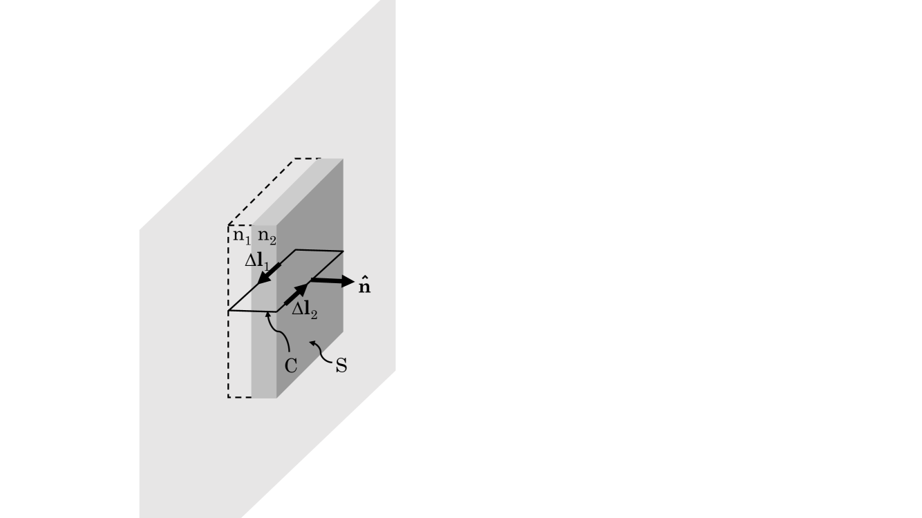
Figure 1: An interface between two magneto-dielectric materials, $\{{\varepsilon}_{1},{\mu}_{1}\}$ and $\{{\varepsilon}_{2},{\mu}_{2}\}$, illustrating the “Gaussian pillbox” and the Stokesian loop across the interface.

Applying Stokes’s theorem for an arbitrary vector ${\bf v}$

$$\oint_{C}{\bf v}\cdot d{\bf l}=\int_{S}(\nabla\times{\bf v})\cdot{\bf\hat{n}}\,da$$ (24)

to Eq. (23), we have

$$\oint_{C}\frac{\nabla\times{\bf A}}{(n_{m}({\bf r}))^{2}}\cdot d{\bf l}=0\,.$$ (25)

We choose the closed contour $C$ in the form of a rectangular Stokesian loop with sides that bisect the two large surfaces and two of the small surfaces on opposite sides of the pillbox shown in Fig. 1. Here, $d{\bf l}$ is a directed line element that lies on the contour, $C$. Then $C$ straddles the material interface. For normal incidence in the plane-wave limit, the field $n_{m}^{-2}\nabla\times{\bf A}$ can be oriented along the long sides of the contour $C$. Performing the contour integration in Eq. (25), the contribution from the short sides of the contour are neglected as the loop is made vanishingly thin and we obtain

$$\frac{1}{({n_{m}}_{1})^{2}}(\nabla\times{\bf A})_{1}\cdot\Delta{\bf l}_{1}+\frac{1}{({n_{m}}_{2})^{2}}(\nabla\times{\bf A})_{2}\cdot\Delta{\bf l}_{2}=0$$ (26)

from the long sides, 1 and 2, of the contour.

On the insident side of the boundary, the field is a composite of the incident and reflected fields. On the other side of the boundary the field is the refracted field. Evaluating Eq. (26) in terms of Eqs. (15)–(17) and using the fact that the line elements $\Delta{\bf l}_{1}$ and $\Delta{\bf l}_{2}$ in Eq. (26) are equal and opposite, we obtain a relation

$$\frac{{n_{e}}_{1}}{{n_{m}}_{1}}(\tilde{A}_{i}-\tilde{A}_{r})=\frac{{n_{e}}_{2}}{{n_{m}}_{2}}\tilde{A}_{R}$$ (27)

between the amplitudes of the incident, reflected, and refracted vector potentials. This relation is usually derived in the Maxwell–Minkowski representation by continuity of the parallel ${\bf H}$ field, cf., Eq. 8.107 of Griffiths. BIGriffiths

In order to derive boundary relations, we need two linearly independent first-order relations. Substituting Eq. (27) into Eq. (21), we have a unique decomposition of Eq. (21)

$$\frac{{n_{e}}_{1}}{{n_{m}}_{1}}\left(\tilde{A}_{i}-\tilde{A}_{r}\right)=\frac{{n_{e}}_{2}}{{n_{m}}_{2}}\tilde{A}_{R}$$ (28)

$$\tilde{A}_{i}+\tilde{A}_{r}=\tilde{A}_{R}$$ (29)

that corresponds to the usual electromagnetic boundary conditions BIMarion ; BIGriffiths ; BIJack ; BIZang .

We eliminate $\tilde{A}_{R}$ from Eq. (28) using Eq. (29) to obtain

$$\frac{\tilde{A}_{r}}{\tilde{A}_{i}}=\frac{{n_{e}}_{1}{n_{m}}_{2}-{n_{e}}_{2}{n_{m}}_{1}}{{n_{e}}_{1}{n_{m}}_{2}+{n_{e}}_{2}{n_{m}}_{1}}\,.$$ (30)

Subsequently, we eliminate $\tilde{A}_{r}$ to get

$$\frac{\tilde{A}_{R}}{\tilde{A}_{i}}=\frac{2{n_{e}}_{1}{n_{m}}_{2}}{{n_{e}}_{1}{n_{m}}_{2}+{n_{e}}_{2}{n_{m}}_{1}}\,.$$ (31)

Eqs. (30) and (31) are the usual Fresnel relations for fields normally incident on a transparent magneto-dielectric material. Although the formulas, Eqs. (30) and (31), are not novel, their derivation from conservation of energy and the wave equation is more general than the usual derivation based on a Minkowski representation of the macroscopic Maxwell equations BIMarion ; BIGriffiths ; BIJack ; BIZang .

Conservation of energy, by itself, is sufficient to derive Eq. (21). However, there are several ways that Eq. (21) can be decomposed into two first-order equations. The application of Stokes’s theorem to the wave equation guarantees uniqueness of the decomposition of the energy balance, Eq. (21), into boundary conditions, Eqs. (28) and (29), and the Fresnel relations, Eqs. (30) and (31), for stationary, transparent, linear, magneto-dielectric, optical materials.

For oblique incidence at an angle $\theta_{i}$ with the normal to the interface, the width of the refracted pulse is $w_{i}({n}_{1}\cos\theta_{R})/({n}_{2}\cos\theta_{i})$. The energy balance, Eq. (20) becomes

$$\frac{{n_{e}}_{1}}{{n_{m}}_{1}}\tilde{A}_{i}^{2}w_{i}=\frac{{n_{e}}_{1}}{{n_{m}}_{1}}\tilde{A}_{r}^{2}w_{i}+\frac{{n_{e}}_{2}}{{n_{m}}_{2}}\tilde{A}_{R}^{2}w_{i}\frac{\cos\theta_{R}}{\cos\theta_{i}}$$ (32)

for our nominally square/rectangular pulse. Then the usual Fresnel relations

$$\frac{\tilde{A}_{r}}{\tilde{A}_{i}}=\frac{{n_{e}}_{1}{n_{m}}_{2}\cos\theta_{i}-{n_{e}}_{2}{n_{m}}_{1}\cos\theta_{R}}{{n_{e}}_{1}{n_{m}}_{2}\cos\theta_{i}+{n_{e}}_{2}{n_{m}}_{1}\cos\theta_{R}}$$ (33)

$$\frac{\tilde{A}_{R}}{\tilde{A}_{i}}=\frac{2{n_{e}}_{1}{n_{m}}_{2}cos\theta_{i}}{{n_{e}}_{1}{n_{m}}_{2}\cos\theta_{i}+{n_{e}}_{2}{n_{m}}_{1}\cos\theta_{R}}$$ (34)

are obtained when we combine the energy balance, Eq. (32), with the relation

$$\tilde{A}_{i}+\tilde{A}_{r}=\tilde{A}_{R}$$ (35)

that is obtained by applying the Stokes’s theorem to the wave equation for the case in which the vector potential is perpendicular to the plane of incidence. Likewise, one obtains

$$\frac{\tilde{A}_{r}}{\tilde{A}_{i}}=\frac{{n_{e}}_{2}{n_{m}}_{1}\cos\theta_{i}-{n_{e}}_{1}{n_{m}}_{2}\cos\theta_{R}}{{n_{e}}_{2}{n_{m}}_{1}\cos\theta_{i}+{n_{e}}_{1}{n_{m}}_{2}\cos\theta_{R}}$$ (36)

$$\frac{\tilde{A}_{R}}{\tilde{A}_{i}}=\frac{2{n_{e}}_{1}{n_{m}}_{2}\cos\theta_{i}}{{n_{e}}_{2}{n_{m}}_{1}\cos\theta_{i}+{n_{e}}_{1}{n_{m}}_{2}\cos\theta_{R}}$$ (37)

by combining the energy balance, Eq. (32), with

$$\cos\theta_{i}(\tilde{A}_{i}-\tilde{A}_{r})=\cos\theta_{R}\tilde{A}_{R}\,.$$ (38)

that is derived from the wave equation by using the Stokes’s theorem in the case of a vector potential that is parallel to the plane of incidence.

In this communication, we obtained the electromagnetic boundary conditions and the Fresnel relations using a derivation that has a well-defined condition of applicability in terms of energy conservation and the validity of the wave equation. The new derivation of the boundary conditions and Fresnel relations is necessary and valuable because the usual derivation is inconsistent with the field equations in some representations of the macroscopic Maxwell field equations for simple linear materials.

References

- (1) P. J. Pritchard, Fox and McDonalds’s Introduction to Fluid Dynamics, 8th ed. (Wiley, New York, 2011).
- (2) J. B. Marion and M. A. Heald, Classical Electromagnetic Radiation, 2nd ed., (Academic Press, Orlando, Florida, 1980).
- (3) Griffiths, D. J., Introduction to Electrodynamics, (Prentice-Hall, Englewood Cliffs, New Jersey, 1981).
- (4) Jackson, J. D., Classical Electrodynamics, 2nd ed., (John Wiley, New York, 1975).
- (5) Zangwill, A., Modern Electrodynamics, (Cambridge University Press, Cambridge, 2013).
- (6) Penfield, P. and Haus, H. A., Electrodynamics of Moving Media, (M.I.T. Press, Cambridge, Massachusetts, 1967).
- (7) Kemp, B. A., “Resolution of the Abraham–Minkowski debate: Implications for the electromagnetic wave theory of light in matter”, J. App. Phys. 109, 111101 (2011).
- (8) Kemp, B. A., “Macroscopic Theory of Optical Momentum”, Prog. Opt. 60, 437–488 (2015).
- (9) Peierls, R., “The momentum of light in a refracting medium”, Proc. R. Soc. Lond. A, 347, 475–491 (1976).
- (10) M. E. Crenshaw, “Electromagnetic momentum and the energy–momentum tensor in a linear medium with magnetic and dielectric properties”, J. Math. Phys. 55, 042901 (2014).
- (11) Møller, C., The Theory of Relativity, (Oxford University Press, London, 1972).
- (12) M. Mansuriur, “The force law of classical electrodynamics: Lorentz versus Einstein and Laub”, Proc. SPIE 8810, Optical Trapping and Micromanipulation X, 88100K (12 Sep 2013).
- (13) C. J. Sheppard and B. A. Kemp, “Optical pressure deduced from energy relations with relativistic formulations of electrodynamics”, Phys. Rev. A , 89, 013825 (2014).