Twist-bend coupling, twist waves and the shape of DNA loops

Abstract

By combining analytical and numerical calculations, we investigate the minimal-energy shape of short DNA loops of approximately $100$ base pairs (bp). We show that in these loops the excess twist density oscillates as a response to an imposed bending stress, as recently found in DNA minicircles and observed in nucleosomal DNA. These twist oscillations, here referred to as twist waves, are due to the coupling between twist and bending deformations, which in turn originates from the asymmetry between DNA major and minor grooves. We introduce a simple analytical variational shape, that reproduces the exact loop energy up to the fourth significant digit, and is in very good agreement with shapes obtained from coarse-grained simulations. We, finally, analyze the loop dynamics at room temperature, and show that the twist waves are robust against thermal fluctuations. They perform a normal diffusive motion, whose origin is briefly discussed.

I Introduction

DNA often forms loops due to the action of proteins, which bind at two distant sites along its sequence and bring them in close contact with each other Alberts et al. (2002). DNA loops play an important role in many biological processes such as transcription, recombination and duplication. The loop length can range from 100 base pairs (bp), in the lac and gal operons of E. Coli Cournac and Plumbridge (2013), to tenths of thousands bp in more complex organisms Krivega and Dean (2012). For lengths much longer than the DNA persistence length, $l_{\text{b}}\approx 50$ nm ($150$ bp), entropic contributions dominate, leading to strong fluctuations in the shape, while in the opposite limit, namely on loops of length comparable to or smaller than $l_{\text{b}}$, the loop assumes approximately its minimal-energy shape. Several studies have focused on the latter regime, not only due to its biological relevance, but also because it allows to investigate the mechanics of highly-deformed DNA Balaeff et al. (1999); Kulić and Schiessel (2003); Sankararaman and Marko (2005); Zhang et al. (2006); Lee et al. (2010); Wilson et al. (2010); Cherstvy (2011); Vafabakhsh and Ha (2012); Le and Kim (2014); Chen et al. (2014); Mulligan et al. (2015).

Mechanical models used for short loops typically neglect sequence-dependent effects, and describe DNA as an isotropic continuous elastic rod. This description fails to account for a coupling interaction present in real DNA, that connects the bending and twisting degrees of freedom, and originates from the asymmetry of the DNA grooves Marko and Siggia (1994). The effect of such a twist-bend coupling interaction on the behavior of DNA at various scales has been recently discussed Nomidis et al. (2017); Skoruppa et al. (2017, 2018); Nomidis et al. (2019); Caraglio et al. (2019). The aim of this paper is to investigate its influence on the structure of short DNA loops. Starting from a simple wormlike chain (WLC) model, in which only the bending degrees of freedom are taken into account, we construct a simple variational ansatz for the loop shape, which we refer to as harmonic loop. This ansatz reproduces very accurately the exact loop shape, which is expressed in terms of elliptic integrals Yamakawa and Stockmayer (1972), while the exact loop energy is reproduced by the harmonic loop ansatz up to four significant digits. The advantage of the variational solution is that it involves simple trigonometric functions, from which various properties of the loop can be easily obtained. Combining with the results of previous work Skoruppa et al. (2018), we have extended the variational solution to more complex DNA models, with anisotropic bending and twist-bend coupling. The comparison with numerical simulations of various coarse-grained model of DNA shows that the harmonic-loop approximation performs extremely well in all cases. As such, it provides a basis for further analysis of the equilibrium and kinetic properties of the DNA loops, which are briefly addressed at the end of this paper.

II DNA elasticity and twist-bend coupling

The simplest continuum model of DNA is the WLC, in which a configuration is described by the tangent vector $\mathbf{\widehat{e}}_{3}(s)$, where $s$ is the curvilinear contour coordinate ($0\leq s\leq L$) and $L$ the total length. The energy takes the following form:

$$\beta E=\frac{l_{\text{b}}}{2}\int_{0}^{L}\text{d}s\left(\frac{\text{d}\mathbf{\widehat{e}}_{3}}{\text{d}s}\right)^{2},$$ (1)

where $\beta=1/k_{\text{B}}T$ is the inverse temperature and $l_{\text{b}}$ the bending persistence length. To include twist, the model can be extended by introducing two additional unit vectors $\mathbf{\widehat{e}}_{1}$ and $\mathbf{\widehat{e}}_{2}$, such that $\{\mathbf{\widehat{e}}_{1},\mathbf{\widehat{e}}_{2},\mathbf{\widehat{e}}_{3}\}$ forms an orthonormal basis. The vectors $\mathbf{\widehat{e}}_{1}$ and $\mathbf{\widehat{e}}_{2}$ keep track of the relative rotation around the $\mathbf{\widehat{e}}_{3}$ axis of neighboring points. In DNA, by convention, $\mathbf{\widehat{e}}_{2}$ connects the backbones of the two strands and $\mathbf{\widehat{e}}_{1}$ points towards the major groove. A generic configuration of the twisted rod can be then parametrized in terms of infinitesimal rotations connecting the orthonormal frame $\{\mathbf{\widehat{e}}_{1},\mathbf{\widehat{e}}_{2},\mathbf{\widehat{e}}_{3}\}$ in $s$ to a neighboring frame in $s+\text{d}s$. This rotation can be mathematically cast into the following differential equation

$$\frac{\text{d}\mathbf{\widehat{e}}_{i}}{\text{d}s}=\left(\mathbf{\Omega}+\omega_{0}\mathbf{\widehat{e}}_{3}\right)\times\mathbf{\widehat{e}}_{i},$$ (2)

where $i=1,2,3$, and $\omega_{0}\approx 1.75$ rad/nm is the intrinsic helical twist density. The solution of the previous equation for $\mathbf{\Omega}=\mathbf{0}$ corresponds to a twisted straight rod ($\mathbf{\widehat{e}}_{3}=\text{const}.$), in which $\mathbf{\widehat{e}}_{1}$ and $\mathbf{\widehat{e}}_{2}$ rotate with angular frequency $\omega_{0}$. One defines the three components of the vector $\mathbf{\Omega}$ along the frame as $\Omega_{i}\equiv\mathbf{\Omega}\cdot\mathbf{\widehat{e}}_{i}$. Here, $\Omega_{1}$ and $\Omega_{2}$ denote the bending densities along the two main axes of the molecule and $\Omega_{3}$ the excess twist density. From the analysis of the symmetry of a DNA molecule, Marko and Siggia derived the following continuum model Marko and Siggia (1994)

$$\beta E=\frac{1}{2}\int_{0}^{L}\!\text{d}s\left(A_{1}\Omega_{1}^{2}+A_{2}\Omega_{2}^{2}+C\Omega_{3}^{2}+2G\Omega_{2}\Omega_{3}\right).$$ (3)

The parameters $A_{1}$ and $A_{2}$ are the stiffnesses associated with bending over the backbone and the grooves, respectively, while $C$ is the intrinsic twist stiffness. Finally, the twist-bend coupling term $G$ leads to a correlation of the strain fields $\Omega_{2}$ and $\Omega_{3}$. Note that from Eq. (2) one obtains

$$\kappa^{2}\equiv\left(\frac{\text{d}\mathbf{\widehat{e}}_{3}}{\text{d}s}\right)^{2}=\Omega_{1}^{2}+\Omega_{2}^{2},$$ (4)

where $\kappa$ is the curvature. Using this relation, and setting $A_{1}=A_{2}=l_{\text{b}}$, while neglecting twist degrees of freedoms, one directly sees that model (3) reduces to (1).

The effect of twist-bend coupling on the mechanical properties of DNA has been investigated in a few recent papers Nomidis et al. (2017); Skoruppa et al. (2017, 2018); Caraglio et al. (2019); Nomidis et al. (2019). An interesting consequence of $G\neq 0$ is the existence of twist oscillations in curved DNA Skoruppa et al. (2018). In Ref. Skoruppa et al. (2018) the following minimal-energy shape of a minicircle was derived

$$\Omega_{1} =\frac{l_{\text{b}}}{A_{1}}\frac{\sin(\omega_{0}s)}{R},$$ (5)

$$\Omega_{2} =\frac{l_{\text{b}}}{\widetilde{A}_{2}}\frac{\cos(\omega_{0}s)}{R},$$

$$\Omega_{3} =-\frac{G}{C}\Omega_{2},$$

where $R$ is the average circle radius and

$$\widetilde{A}_{2}=A_{2}\left(1-\frac{G^{2}}{A_{2}C}\right),$$ (6)

an effective bending stiffness. Finally, $l_{\text{b}}$ is the bending persistence length, which within model (3) is given by

$$\frac{1}{l_{\text{b}}}=\frac{1}{2}\left(\frac{1}{A_{1}}+\frac{1}{\widetilde{A}_{2}}\right),$$ (7)

i.e., the harmonic mean of the two stiffnesses Nomidis et al. (2017). The oscillations in the bending densities $\Omega_{1}$ and $\Omega_{2}$ arise from the geometrical constraints of the system, which in turn induce oscillations in the twist density $\Omega_{3}$ from the presence of twist-bend coupling ($G\neq 0$). These twist waves have been indeed observed in X-ray crystallographic structures of DNA bound to histone proteins Skoruppa et al. (2018). While Eq. (5) describes a torsionally-relaxed minicircle, this solution has also been recently extended to minicircles which are either over- or undertwisted Caraglio et al. (2019).

III Harmonic loops in the WLC model

Considerable attention has been devoted to the study of structural and dynamical properties of DNA loops in the past two decades Balaeff et al. (1999); Kulić and Schiessel (2003); Sankararaman and Marko (2005); Zhang et al. (2006); Lee et al. (2010); Wilson et al. (2010); Cherstvy (2011); Vafabakhsh and Ha (2012); Le and Kim (2014); Chen et al. (2014); Mulligan et al. (2015). Already in the early 70s, Yamakawa and Stockmayer Yamakawa and Stockmayer (1972) discussed the minimal-energy configuration of a semiflexible loop within the framework of the isotropic WLC [Eq. (1)]. The exact shape thus obtained is expressed in terms of inverse elliptic integrals, and its derivation is outlined in Appendix A. Although exact, these expressions are not easy to handle, therefore simpler approximate loop configurations have also been considered. For instance, in the context of DNA looping in the nucleosome, Kulic and Schiessel Kulić and Schiessel (2003) introduced a so-called circle-line approximation, in which the DNA conformation is built from straight segments and arcs of circles. A similar approach was followed by Sankararaman and Marko Sankararaman and Marko (2005), who studied DNA loops under tension. In the same spirit, we introduce here a different approximate shape for the loop, which we refer to as harmonic loop. Though still simple, it is found to be more accurate, and will allow us to construct a full analytical shape for the anisotropic model (3). From that, we can directly estimate several quantities of interest, such as twist oscillations, curvature variation and minimal energy.

As the problem is two-dimensional, one can describe the shape of the loop using a single parameter $\theta(s)$, defined as the angle the tangent $\mathbf{\widehat{e}}_{3}$ forms with the x-axis:

$$\mathbf{\widehat{e}}_{3}=\cos\theta\,\mathbf{\widehat{x}}+\sin\theta\,\mathbf{\widehat{y}},$$ (8)

where the unit vectors $\mathbf{\widehat{x}}$ and $\mathbf{\widehat{y}}$ lie on the plane of the loop. Since no rotational constraints are applied at the loop endpoints, the curvature $\kappa=|\text{d}\theta/\text{d}s|$ [see Eq. (4)] must vanish at the boundaries, hence

$$\frac{\text{d}\theta(0)}{\text{d}s}=\frac{\text{d}\theta(L)}{\text{d}s}=0.$$ (9)

A simple ansatz fulfilling these boundary conditions is

$$\frac{\text{d}\theta^{(1)}}{\text{d}s}=\frac{\pi c_{1}}{L}\sin\left(\frac{\pi s}{L}\right),$$ (10)

which we refer to as first-order harmonic loop. Here, the dimensionless constant $c_{1}$ can be fixed by requiring that the endpoints coincide. This constraint is discussed in Appendix B and can be cast in the form $J_{0}(c_{1})=0$, with $J_{0}$ being the zeroth-order Bessel function of the first kind [see Eq. (30)]. The parameter $c_{1}$ is, thus, the first root of $J_{0}$, which is known to a high degree of accuracy, $c_{1}=2.40482556$.

Figure 1(a) shows with a red dashed line the loop shape, obtained by integrating Eq. (10), plugging into Eq. (8) and integrating once more. The red dashed line in Fig. 1(b) shows a plot of Eq. (10), multiplied by the loop length $L$, so as to render it dimensionless. For comparison, the same graphs show as blue solid lines the shapes and curvature corresponding to the exact solution (26) Yamakawa and Stockmayer (1972). There is a reasonable overall agreement between the exact solution and first-harmonic approximation. Plugging Eqs. (10) and (8) into Eq. (1), we find the following energy for the harmonic loop

$$\beta E^{(1)}_{\text{HL}}=\left(\frac{\pi c_{1}}{2}\right)^{2}\frac{l_{\text{b}}}{L}=14.2694\,\frac{l_{\text{b}}}{L},$$ (11)

which is very close to the exact value $\beta E_{\text{exact}}=14.0550\,(l_{\text{b}}/L)$ of the Yamakawa-Stockmayer solution Yamakawa and Stockmayer (1972). The value in Eq. (11) improves upon the “circle-line” approximation of Ref. Kulić and Schiessel (2003), which gives $\beta E_{\text{CL}}=15.70\,(l_{\text{b}}/L)$.

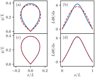
Figure 1: Minimal-energy loop shape (left) and curvature as a function of the rescaled arc-length coordinate $s/L$ (right). Blue solid lines are obtained from the exact solution (26) Yamakawa and Stockmayer (1972), while red dashed lines show (a,b) the first- and (c,d) third-harmonic solutions, corresponding to Eqs. (10) and (12), respectively.

Our approximation scheme can be systematically improved by including higher-order terms. We consider the following variational ansatz

$$\frac{\text{d}\theta^{(3)}}{\text{d}s}=\frac{\pi}{L}\left[c_{1}\sin\left(\frac{\pi s}{L}\right)+c_{3}\sin\left(\frac{3\pi s}{L}\right)\right],$$ (12)

which extends Eq. (10) by adding an additional harmonic, consistent with the symmetry of the solution (we require $\text{d}\theta/\text{d}s$ to be symmetric around $s=L/2$, which excludes all even harmonics with frequency $2\pi n/L$ and $n$ integer). The two parameters $c_{1}$ and $c_{3}$ are now fixed by requiring both the closure of the loop and the energy minimization of Eq. (1). We, thus, find the values $c_{1}=2.3703$ and $c_{3}=-0.2808$ (more details can be found in Appendix B). The resulting shape and rescaled curvatures are shown as dashed red lines in Fig. 1(c) and (d), revealing an excellent agreement with the exact solution (solid blue line). The energy is found to be

$$\beta E^{(3)}_{\text{HL}}=\frac{\pi^{2}\left(c_{1}^{2}+c_{3}^{2}\right)}{4}\,\frac{l_{\text{b}}}{L}=14.0572\,\frac{l_{\text{b}}}{L},$$ (13)

which matches the exact solution up to four significant digits. The ansatzes of Eqs. (10) and (12) can be extended to the case where the end-points are fixed at some finite distance $d$ (see Appendix B). Table 1 summarizes the optimal values of the coefficients $c_{1}$ and $c_{3}$ for the first- and third-harmonic approximations for some selected values of $d$. A comparison between the exact results and the harmonic approximations shows that the latter become even better with increasing $d$, i.e., as the distance between the end-points increases (for more details, see Appendix B).

Table 1: Comparison between harmonic-loop energies and the exact values for three different “loop” geometries with varying distance $d$ between the endpoints. $d=0$ corresponds to the closed loops of Fig. 1.

d		$c_{1}$	$c_{3}$	$\beta EL/l_{\text{b}}$	Error(%)
$0$	1st	2.4048	–	14.2694	1.53
	3rd	2.3703	-0.2808	14.0572	0.02
	Exact			14.0550
$L/10$	1st	2.2187	–	12.1459	0.98
	3rd	2.1977	-0.2135	12.0295	0.02
	Exact			12.0286
$L/5$	1st	2.0415	–	10.2837	0.63
	3rd	2.0288	-0.1612	10.2198	$<$0.01
	Exact	–	–	10.2194

From the simple analytical, but accurate, form of the loop shape one can easily obtain several estimates of the loop properties. Let us consider, for instance, the curvature $\kappa(s)=\text{d}\theta/\text{d}s$, which reaches its maximum value $\kappa_{\text{max}}$ at the apex $s=L/2$ of the loop. From the third-harmonic approximation (12), one finds

$$\kappa_{\max}=\frac{\pi}{L}\left(c_{1}-c_{3}\right).$$ (14)

Next, we wish to estimate the curvature $\kappa_{\text{turn}}$ at a distance of one helical repeat from the apex, i.e., at $s=L/2+2\pi/\omega_{0}$. Again, from Eq. (12) this is found to be

$$\kappa_{\text{turn}}=\frac{\pi}{L}\left(c_{1}\cos\alpha-c_{3}\cos 3\alpha\right),$$ (15)

where we introduced the angle $\alpha\equiv 2\pi^{2}/\omega_{0}L$. Finally, combining Eqs. (14) and (15), one finds the maximal curvature drop

$$\frac{\Delta\kappa}{\kappa_{\text{max}}}\equiv\frac{\kappa_{\text{max}}-\kappa_{\text{turn}}}{\kappa_{\text{max}}}=1-\frac{c_{1}\cos\alpha-c_{3}\cos 3\alpha}{c_{1}-c_{3}}.$$ (16)

Consulting Table 1 for $d=0$ and considering a DNA loop of 100 bp ($L=34$ nm), yields $\kappa_{\text{max}}=0.24\,\text{nm}^{-1}$ and $\Delta\kappa/\kappa_{\text{max}}\approx 0.097$.

IV Minimal-energy configuration of DNA loops: Modulated twist waves

IV.1 Analytical results

The analysis of Eq. (16) for a loop of $100$ bp reveals a rather modest curvature drop at the scale of the helical-repeat length. This allows us to use Eq. (5), derived for a minicircle of average radius $R$, by replacing $1/R$ with the modulated harmonic-loop curvature. For instance, combining Eq. (10) with (5) yields the first-harmonic solution

$$\Omega^{(1)}_{1} =\frac{l_{\text{b}}}{A_{1}}\,\frac{\pi c_{1}}{L}\sin\left(\frac{\pi s}{L}\right)\sin(\omega_{0}s+\phi),$$ (17)

$$\Omega^{(1)}_{2} =\frac{l_{\text{b}}}{\widetilde{A}_{2}}\frac{\pi c_{1}}{L}\sin\left(\frac{\pi s}{L}\right)\cos(\omega_{0}s+\phi),$$

$$\Omega^{(1)}_{3} =-\frac{G}{C}\Omega^{(1)}_{2},$$

where a phase constant $\phi$ has been added, accounting for the torsional freedom of DNA at the boundaries (torsionally-unconstrained ends). Similarly, one can combine Eq. (5) with Eq. (12), so as to construct a more accurate approximation

$$\Omega^{(3)}_{1} =\frac{l_{\text{b}}}{A_{1}}\frac{\pi}{L}\left[c_{1}\sin\left(\frac{\pi s}{L}\right)+c_{3}\sin\left(\frac{3\pi s}{L}\right)\right]\sin(\omega_{0}s+\phi),$$ (18)

$$\Omega^{(3)}_{2} =\frac{l_{\text{b}}}{\widetilde{A}_{2}}\frac{\pi}{L}\left[c_{1}\sin\left(\frac{\pi s}{L}\right)+c_{3}\sin\left(\frac{3\pi s}{L}\right)\right]\cos(\omega_{0}s+\phi),$$

$$\Omega^{(3)}_{3} =-\frac{G}{C}\Omega^{(3)}_{2}.$$

Similar to the minicircle case [Eqs. (5)], one notices the emergence of twist waves, originating from twist-bend coupling ($G\neq 0$). In this case, however, these are modulated by the varying curvature, which vanishes at the loop edges and is maximal at the loop apex.

By plugging Eqs. (17) into Eq. (3) and performing the integration in $s$, one can compute the total energy of the loop (see Appendix C for details)

$$\beta E^{(1)}_{\text{HL}}=\left(\frac{\pi c_{1}}{2}\right)^{2}\frac{l_{\text{b}}}{L}+\beta\Delta E(\phi).$$ (19)

This expression is identical to Eq. (11) with the addition of a boundary term $\Delta E(\phi)$ depending on the phase $\phi$. One can show that this term is negligible for loops of about 100 bp, such as those considered here ($|\Delta E|/E^{(1)}_{\text{HL}}\sim 10^{-4}$). We, thus, conclude that the energy is quasi-degenerate, corresponding to an invariance of the double helix with respect to a global rotation $\phi$ around its axis. A similar conclusion holds for the third-harmonic approximation.

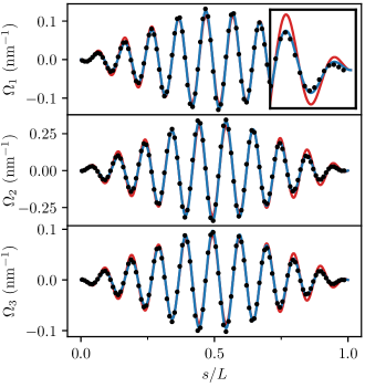
Figure 2: Plots of the bending ($\Omega_{1}$ and $\Omega_{2}$) and twist ($\Omega_{3}$) densities of a closed triad-model loop, as functions of the reduced arc-length $s/L$. The black circles are low-temperature Monte Carlo simulations of the triad model (with $104$ bp), while the red and blue solid lines are the first- [Eq. (17)] and third-harmonic [Eq. (18)] ansatzes, respectively. The inset zooms into the one end of the loop, and reveals that the third-harmonic ansatz more accurately reproduces the data. The stiffness constants were chosen as $A_{1}=81~{}\text{nm}$, $A_{2}=39~{}\text{nm}$, $C=105~{}\text{nm}$ and $G=30~{}\text{nm}$, calculated in Ref. Skoruppa et al. (2017) from the oxDNA2 model. The global phase $\phi=4.02$ rad is the only fitting parameter.

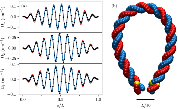
Figure 3: (a) Similar to Fig. 2, but with the data obtained from low-temperature oxDNA2 simulations (black points). For the harmonic approximations [Eqs. (17) and (18), shown with red and blue lines, respectively] we used the same values as in Fig. 2, extracted from oxDNA2 simulations Skoruppa et al. (2017). Once more, the global phase $\phi=1.70$ rad is the only fitting parameter. (b) Actual configuration of the loop from which the plots in (a) were produced. The yellow points indicate the bp that were tethered to two fixed points in space by means of harmonic springs, effectively fixing the end distance (center-of-mass distance between the two pairs of yellow beads) at $d=L/10$.

Finally, from Eq. (17) [or Eq. (18)] one can estimate the curvature at the loop apex

$$\widetilde{\kappa}_{\max}\equiv\left.\sqrt{\Omega_{1}^{2}+\Omega_{2}^{2}}\right|_{s=L/2},$$ (20)

and compare it with the corresponding WLC loop curvature $\kappa_{\max}=\pi c_{1}/L$ [Eq. (14)], derived in Sec. III. $\widetilde{\kappa}_{\max}$ depends on $\phi$ and, using some simple algebra, one can show that the ratio $\widetilde{\kappa}_{\max}/\kappa_{\max}$ is bounded within the interval

$$\frac{2\widetilde{A}_{2}}{A_{1}+\widetilde{A}_{2}}\leq\frac{\widetilde{\kappa}_{\max}}{\kappa_{\max}}\leq\frac{2A_{1}}{A_{1}+\widetilde{A}_{2}},$$ (21)

(note that the same expression is valid both for the first- and third-harmonic approximation). Equation (21) shows that $\widetilde{\kappa}_{\max}$ does not, in general, coincide with the WLC loop apex curvature $\kappa_{\max}$. The latter has been obtained for a perfectly planar loop, however the solution (5) [and, thus, also (17) and (18)] describes an almost-planar curve with small off-planar oscillations Skoruppa et al. (2018), which are induced by the combined effect of bending anisotropy and twist-bend coupling.

IV.2 Numerical analysis

In order to test the validity of Eqs. (17) and (18), we performed Monte Carlo simulations of a “triad model”, which is derived from a direct discretization of Eq. (3). A DNA molecule with $N$ base pairs is represented by $N$ beads, each carrying a set of three orthogonal unit vectors forming the triad $\{\mathbf{\widehat{\bf e}}_{1},\mathbf{\widehat{\bf e}}_{2},\mathbf{\widehat{\bf e}}_{3}\}$, with $\mathbf{\widehat{\bf e}}_{3}$ being the tangent, and hence pointing towards the next bead. Consecutive beads are separated by a fixed distance $a=0.34$ nm, corresponding to the average base pair distance of DNA. The simulations are performed at sufficiently-low temperature, so that the system converges to its lowest-energy state (more details can be found in Ref. Caraglio et al. (2019)). Figure 2 shows the bending densities ($\Omega_{1}$, $\Omega_{2}$) and excess twist density ($\Omega_{3}$) as functions of the rescaled arc-length coordinate $s/L$ obtained from Monte Carlo simulations of a loop of $104$ bp (black circles). The lines are plots of Eqs. (17) (red) and Eqs. (18) (blue). The only adjustable parameter is the global phase $\phi$, as the stiffness constants $A_{1}$, $A_{2}$, $C$ and $G$ are input parameters (see caption of Fig. 2), while $c_{1}$ and $c_{3}$ are the universal constants given in Table 1. Figure 2 shows an excellent agreement between both harmonic approximations and the Monte Carlo data. As in the case of WLC loops shown in Fig. 1, the first-harmonic approximation overestimates the curvature at the loops ends (see inset of Fig. 2). The maximal excess twist in a loop with $104$ bp is $\max|\Omega_{3}|\approx 0.1~{}\text{nm}^{-1}$, which, compared to the average intrinsic twist $\omega_{0}=1.75~{}\text{nm}^{-1}$, corresponds to a deviation of 6% from $\omega_{0}$. Finally, note that the maximum curvature $\kappa_{\text{max}}=0.24$ nm^-1, predicted by Eq. (14), is once more substantially lower than the total curvature in the middle of the loop of the triad model, which from the numerical data is found to be $\widetilde{\kappa}_{\max}=0.34$ nm^-1. This is due to off-planar oscillations along the loop, as discussed above [Eq. (21)].

To further corroborate the harmonic-loop approximations, we performed low-temperature ($T=1$ K) computer simulations of 100-bp oxDNA loops (Fig. 3). OxDNA is a coarse-grained model, which describes DNA as two intertwined strands of rigid nucleotides Ouldridge et al. (2010). For the simulations we used the latest version oxDNA2 Snodin et al. (2015), which was recently found to have a substantially-nonzero twist-bend coupling constant Skoruppa et al. (2017). The electrostatic interactions are implicitly modelled through a Debye-Hückel potential. The initial configuration was a torsionally-relaxed helix, with the molecular axis having the shape of Eq. (12). To avoid undesired interactions between the two DNA ends, we constrained them at a nonzero distance $d=L/10$ by means of strong harmonic bonds. These bonds connect the center of mass of the fifth base pair at each end (yellow beads in Fig. 3b) with a fixed point in space (distance $d$ between the two centers of mass). This is to prevent end-point denaturation effects, which can affect in particular the room temperature simulations, such as those presented in Section V. The simulations were performed with the recently-developed LAMMPS Plimpton (1995) implementation of the oxDNA model Henrich et al. (2018). Figure 3a shows $\Omega_{i}$ as functions of the arc-length parameter, and once more reveals an excellent agreement with the harmonic approximations. Again, the only free parameter is the global phase $\phi$, as the stiffness constants $A_{1}$, $A_{2}$, $C$ and $G$ have already been calculated for oxDNA2 in Ref. Skoruppa et al. (2017), while $c_{1}$ and $c_{3}$ were taken from Table 1 with $d=L/10$.

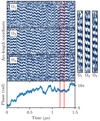
Figure 4: Kymogram plots of the time evolution of the deformation densities $\Omega_{i}$ along an oxDNA loop (top three panels), together with the corresponding global phase (bottom panel), obtained from room-temperature simulations. The right subplots show a zoom in the region marked by red lines, revealing that the correlations predicted by Eqs. (17) and (18) survive the effect of thermal fluctuations. In the kymographs, the blue and white regions correspond to positive and negative values of the $\Omega_{i}$’s, respectively.

V Effect of Thermal Fluctuations

Having analyzed the minimal-energy conformation of DNA loops, we now consider the effect of thermal fluctuations. For this purpose, we simulated oxDNA loops using the same setup as discussed in Section IV, with the only difference that the temperature now is $T=300$ K. Figure 4 shows kymogram traces of $\Omega_{i}$ along the DNA loop as functions of time. To better distinguish regions of predominantly-positive $\Omega_{i}$ from those of negative $\Omega_{i}$, we applied a Gaussian filter on both the spatial ($3$-bp variance) and temporal direction (4-frame variance), and used a binary color code (white for negative and blue for positive values). At the loop ends, the image is more blurred due to the thermal fluctuations dominating over the wave amplitude, as expected from the vanishing curvature. In the central region, however, clear wave patterns are visible in the bending and twist deformations, with a period following that of the DNA double helix, in line with the ground-state solutions (17) and (18). In order to better compare the relative phase among $\Omega_{i}$, the side figure shows a zoom-in of the three variables at a given small time interval (red vertical lines), further confirming the validity of Eqs. (17) and (18). We, thus, conclude that, even under the effect of thermal fluctuations, not only do the bending and twist degrees of freedom retain their modulated-wave shape, but also preserve their relative phase difference.

The global phase $\phi$ at the bottom of Fig. 4 was obtained by keeping track of the orientation of the two loop ends, which yielded the phase difference $\Delta\phi$ between successive time steps. The initial phase was determined from the Fourier analysis of the $\Omega_{2}$ wave of the first frame. The mean-squared displacement of $\phi$ grows linearly with time, as shown in Fig. 5, yielding a diffusion constant of $D=121~{}\text{rad}^{2}/\mu s$. Note that, the simulation time scale depends on the value of the Langevin damping parameter, which in this case was $6.06$ ps. The origin of the observed diffusive behavior stems from the very weak contribution of $\Delta E(\phi)$ to Eq. (19), as discussed in Section IV, indicating that the phase $\phi$ moves on an almost-flat energy landscape.

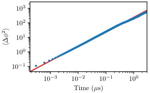
Figure 5: Time evolution of the mean-squared displacement of the phase $\phi$ (blue points), averaged over six independent oxDNA2 runs, which reveals regular diffusion. Fitting to $\langle\Delta\phi^{2}\rangle=2Dt$ (solid red line), we obtain the value $D=121~{}\text{rad}^{2}/\mu s$ for the diffusion coefficient.

VI Conclusion

In this paper, we have investigated the shape and dynamics of short DNA loops, i.e., consisting of about 100 bp. Such loops are generated in vivo by DNA binding proteins. We have developed a two-parameter variational explicit solution for the minimal energy shape of the loop, which we refer to as harmonic loop, being described by a combination of simple trigonometric functions. This solution was found to be in excellent agreement with numerical simulations of two different coarse-grained models, and reproduces the exact WLC energy Yamakawa and Stockmayer (1972) up to four significant digits. We focused particularly on the effect of twist-bend coupling, which is an interaction arising from the DNA grooves asymmetry Marko and Siggia (1994). As recently discussed in the case of DNA minicircles and nucleosomal DNA Skoruppa et al. (2018), we found that also in DNA loops the bending deformation induces twist waves, i.e., twist oscillations following the periodicity of the helical pitch. Differently from the minicircle case, in the loops discussed here twist waves have a modulated amplitude, which is maximal at the loop apex and vanishes at the two ends. For a loop of 100 bp the maximal degree of over- and undertwisting close to the apex was estimated to be $6\%$ relative to the intrinsic double-helix twist $\omega_{0}$.

As an alternative approach, we could have used the numerically exact solution by Yamakawa and Stockmayer Yamakawa and Stockmayer (1972) to obtain the radius of curvature, $R(s)$, of the loop as a function of the curvilinear coordinate $s$. The loop shape for the model (3) is then obtained by replacing the numerical values of $R(s)$ into Eqs. (5). This approach, however, would not allow for a direct estimate of derived quantities, such as twist oscillations, curvature variation and minimal energy. The harmonic-loop approximation provides simple, yet accurate, expressions for these quantities, see e.g., Eqs. (14), (19) and (21).

Finally, we considered the loop kinetics in oxDNA simulations at room temperature. Interestingly, the bending and twist waves were not masked by the presence of thermal fluctuations, and performed a correlated motion over the whole length of the loop. This allowed us to characterize the kinetics in terms of a single parameter $\phi(t)$, describing the absolute phase of the waves. This was found to follow a simple diffusive motion, which originates from the ground-state quasi-degeneracy in $\phi$. These findings, and particularly the simplicity of our solution, may form the basis for more complex analytical calculations that involve strongly-bent DNA, such as under the action of DNA-binding proteins.

Appendix A Exact variational calculus

In what follows, we briefly review the derivation of the exact solution by Yamakawa and Stockmayer Yamakawa and Stockmayer (1972). Owing to the symmetry of the problem, a sufficient condition in order to ensure that the loop will close is to require that the apex of the loop has not shifted along the x-axis. Let us define $\mathbf{R}$ the vector connecting the end-point with the loop apex. We require that

$$\mathbf{R}\cdot\mathbf{\widehat{x}}=\int_{0}^{L/2}\mathbf{\widehat{e}}_{3}\cdot\mathbf{\widehat{x}}\,\text{d}s=\int_{0}^{L/2}\cos[\theta(s)]\,\text{d}s=0.$$ (22)

The determination of the minimum energy under the above constraint can be performed by introducing a Lagrange multiplier $\mu$ as follows

$$\beta E=\int_{0}^{L}\left(\frac{A\dot{\theta}^{2}}{2}-\mu\cos\theta\right)\text{d}s,$$ (23)

where $\dot{\theta}\equiv\text{d}\theta/\text{d}s$. The Euler-Lagrange equation then becomes

$$A\ddot{\theta}=\mu\sin\theta,$$ (24)

which has the following integral of motion

$$\frac{A}{2}\dot{\theta}^{2}+\mu\cos\theta=\Gamma.$$ (25)

Interpreting $\theta$ as the coordinate of a fictitious particle with mass $A$, and $s$ as the time variable, Eq. (24) can be viewed as the equation of motion for a particle in the potential $U(\theta)=\mu\cos\theta$, describing the dynamics of a pendulum under gravity, where $\mu$ plays the role of gravitational acceleration. This is the well-known Kirchhoff kinetic analogy, showing that the static conformations of elastic rods are formally equivalent to the kinetic of spinning tops. In this analogy Eq. (25) expresses the conservation of the mechanical energy. The boundary conditions (9) imply zero velocity at the begin and end point, hence $\Gamma=\mu\cos\alpha$, with $\theta(0)=\alpha$ and $\theta(L)=2\pi-\alpha$. The trajectory $\theta(s)$ is then given by Yamakawa and Stockmayer (1972)

$$F\left(\frac{\pi-\theta(s)}{2},k\right)=F\left(\frac{\pi-\alpha}{2},k\right)-\sqrt{\frac{\mu}{A}}\,\frac{s}{k},$$ (26)

where $k^{-1}\equiv\cos(\alpha/2)$ and $F(\phi,k)$ is the incomplete Elliptic integral of the first kind

$$F(\phi,k)=\int_{0}^{\phi}\frac{d\omega}{\sqrt{1-k^{2}\sin^{2}\omega}}.$$ (27)

The values for $\alpha$ and $\mu$ are fixed by requiring that the loop has length $L$ and that it is closed, e.g., that $\theta(s)$ satisfies (22).

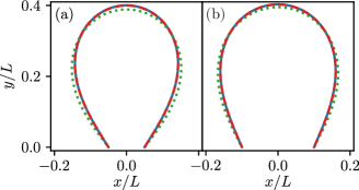
Figure 6: Comparison of the shape among the one-harmonic approximation (10) (dotted green lines), two-harmonics approximation (12) (dashed red lines) and the exact solution (solid blue lines), with the two ends of the loop being fixed at a distance $L/10$ (a) and $L/5$ (b).

Appendix B Harmonic loop ansatz

The potential energy of the pendulum has a minimum at $\theta=\pi$, corresponding to the loop apex. As a simple approximation we expand this potential around the minimum, which gives

$$U(\theta)=\mu\cos\theta\approx\mu\left[-1+\frac{(\theta-\pi)^{2}}{2}\right],$$ (28)

corresponding to a pendulum in the small-oscillation limit. The solution with $\theta(L/2)=\pi$ and zero velocity at the end points is then

$$\theta^{(1)}(s)=\pi-c_{1}\cos\left(\frac{\pi s}{L}\right).$$ (29)

Note that the derivative of this solution is given by Eq. (10). Plugging the above equation in (22), and with a simple change of variables, one obtains

$$\int_{0}^{\pi/2}\cos(c_{1}\cos\phi)\text{d}\phi\equiv\frac{\pi}{2}\,J_{0}(c_{1})=0,$$ (30)

where $J_{0}$ is the zeroth-order Bessel function of the first kind . This constraint, thus, fixes the constant to the smallest zero of $J_{0}$: $c_{1}=2.4048$.

Similarly, the third-order harmonic loop is obtained from the following trial function

$$\theta^{(3)}(s)=\pi-c_{1}\cos\left(\frac{\pi s}{L}\right)-\frac{c_{3}}{3}\cos\left(\frac{3\pi s}{L}\right),$$ (31)

with its derivative being given by Eq. (12), and the loop-closure constraint taking the form

$$\int_{0}^{\pi/2}\cos\left[c_{1}\cos\phi+\frac{c_{3}}{3}\cos(3\phi)\right]\text{d}\phi=0.$$ (32)

Imposing this constraint, together with the minimization of the elastic energy (1), we obtain the values $c_{1}=2.3703$ and $c_{3}=-0.2808$ for the constants.

The above calculation can be easily generalized to open loops whose end-points are kept at some finite distance $d$. In that case, the form of the harmonic solutions (29) and (31) remains identical, but the right-hand sides of Eqs. (30) and (32) are set to the nonzero value $-d/2L$ ($x$-projection of vector pointing from the right end of the loop to the apex). As the endpoints distance increases, the harmonic ansatz becomes a more accurate approximation of the full solution (see Fig. 6). This is because, as $d$ increases, $\theta(s)$ varies within an interval getting closer to $\theta=\pi$, hence the small-angle approximation (28) becomes increasingly more accurate. This is also reflected in the improved accuracy of the data in Table 1 upon increasing $d$.

Appendix C Calculation of the energy

In this section we present some additional details over the loop-energy calculation. For simplicity, we limit the analysis to the first-harmonic approximation, as the third-harmonic case follows the same approach. The energy density, obtained from Eq. (17), becomes (to simplify the notation we drop the superscript in $\Omega_{i}^{(1)}$)

$$\frac{1}{2}\left(A_{1}\Omega_{1}^{2}+A_{2}\Omega_{2}^{2}+C\Omega_{3}^{2}+2G\Omega_{2}\Omega_{3}\right)=\frac{1}{2}\left(A_{1}\Omega_{1}^{2}+\widetilde{A}_{2}\Omega_{2}^{2}\right)=\left(\frac{l_{\text{b}}\pi c_{1}}{L}\right)^{2}\sin^{2}\left(\frac{\pi s}{L}\right)\left[\frac{\sin^{2}(\omega_{0}s+\phi)}{2A_{1}}+\frac{\cos^{2}(\omega_{0}s+\phi)}{2\widetilde{A}_{2}}\right].$$ (33)

To obtain the expression in the second equality we have used Eq. (17) to eliminate $\Omega_{3}$. Interestingly, this relation shows that the energy is identical to that of a pure bending deformation with a reduced stiffness $\widetilde{A}_{2}$ instead of $A_{2}$. To proceed, we use the trigonometric identities

$$4\sin^{2}\left(\frac{\pi s}{L}\right)\sin^{2}(\omega_{0}s+\phi) =1-\cos\frac{2\pi s}{L}-\cos\left(2\omega_{0}s+2\phi\right)+\frac{1}{2}\cos\left[2\left(\omega_{0}-\frac{\pi}{L}\right)s+2\phi\right]+\frac{1}{2}\cos\left[2\left(\omega_{0}+\frac{\pi}{L}\right)s+2\phi\right],$$ (34)

$$4\sin^{2}\left(\frac{\pi s}{L}\right)\cos^{2}(\omega_{0}s+\phi) =1-\cos\frac{2\pi s}{L}+\cos\left(2\omega_{0}s+2\phi\right)-\frac{1}{2}\cos\left[2\left(\omega_{0}-\frac{\pi}{L}\right)s+2\phi\right]-\frac{1}{2}\cos\left[2\left(\omega_{0}+\frac{\pi}{L}\right)s+2\phi\right],$$ (35)

To complete the calculation of the energy, one needs to integrate in $0\leq s\leq L$. The integral of $\cos(2\pi s/L)$ vanishes; inserting Eqs. (34) and (35) in Eq. (33) and integrating, one finally gets

$$\beta E^{(1)}_{\text{HL}}=\frac{1}{2}\left(\frac{l_{\text{b}}\pi c_{1}}{L}\right)^{2}\frac{L}{4}\left(\frac{1}{A_{1}}+\frac{1}{\widetilde{A}_{2}}\right)+\beta\Delta E(\phi).$$ (36)

where we have separated the dominant contribution, obtained from the integration of the constant term in the right-hand side of Eqs. (34) and (35), from the part which depends on the phase $\phi$. The former is an extensive term, giving a contribution proportional to $L$, while the integration of the $\phi$-dependent part gives a very small boundary contribution. Finally, using the definition (7) of $l_{\text{b}}$, one sees that Eq. (36) reduces to Eq. (19) of the main text.

References

- Alberts et al. (2002) B. Alberts, D. Bray, J. Lewis, M. Raff, K. Roberts, and J. Watson, Molecular Biology of the Cell, 4th ed. (Garland, 2002).
- Cournac and Plumbridge (2013) A. Cournac and J. Plumbridge, J. Bacteriol. 195, 1109 (2013).
- Krivega and Dean (2012) I. Krivega and A. Dean, Curr. Op. Gen. & dev. 22, 79 (2012).
- Balaeff et al. (1999) A. Balaeff, L. Mahadevan, and K. Schulten, Phys. Rev. Lett. 83, 4900 (1999).
- Kulić and Schiessel (2003) I. Kulić and H. Schiessel, Biophys. J. 84, 3197 (2003).
- Sankararaman and Marko (2005) S. Sankararaman and J. F. Marko, Phys. Rev. E 71, 021911 (2005).
- Zhang et al. (2006) Y. Zhang, A. E. McEwen, D. M. Crothers, and S. D. Levene, Biophys. J. 90, 1903 (2006).
- Lee et al. (2010) O.-c. Lee, J.-H. Jeon, and W. Sung, Phys. Rev. E 81, 021906 (2010).
- Wilson et al. (2010) D. P. Wilson, A. V. Tkachenko, and J.-C. Meiners, Europhys. Lett. 89, 58005 (2010).
- Cherstvy (2011) A. G. Cherstvy, J. Biol. Phys. 37, 227 (2011).
- Vafabakhsh and Ha (2012) R. Vafabakhsh and T. Ha, Science 337, 1097 (2012).
- Le and Kim (2014) T. T. Le and H. D. Kim, Nucleic Acids Res. 42, 10786 (2014).
- Chen et al. (2014) Y.-J. Chen, S. Johnson, P. Mulligan, A. J. Spakowitz, and R. Phillips, Proc. Natl. Acad. Sci. USA 111, 17396 (2014).
- Mulligan et al. (2015) P. J. Mulligan, Y.-J. Chen, R. Phillips, and A. J. Spakowitz, Biophy. J. 109, 618 (2015).
- Marko and Siggia (1994) J. Marko and E. Siggia, Macromolecules 27, 981 (1994).
- Nomidis et al. (2017) S. K. Nomidis, F. Kriegel, W. Vanderlinden, J. Lipfert, and E. Carlon, Phys. Rev. Lett. 118, 217801 (2017).
- Skoruppa et al. (2017) E. Skoruppa, M. Laleman, S. Nomidis, and E. Carlon, J. Chem. Phys. 146, 214902 (2017).
- Skoruppa et al. (2018) E. Skoruppa, S. Nomidis, J. F. Marko, and E. Carlon, Phys. Rev. Lett. 121, 088101 (2018).
- Nomidis et al. (2019) S. K. Nomidis, E. Skoruppa, E. Carlon, and J. F. Marko, Phys. Rev. E 99, 032414 (2019).
- Caraglio et al. (2019) M. Caraglio, E. Skoruppa, and E. Carlon, J. Chem. Phys 150, 135101 (2019).
- Yamakawa and Stockmayer (1972) H. Yamakawa and W. Stockmayer, J. Chem. Phys. 57, 2843 (1972).
- Ouldridge et al. (2010) T. E. Ouldridge, A. A. Louis, and J. P. Doye, Phys. Rev. Lett. 104, 178101 (2010).
- Snodin et al. (2015) B. E. Snodin, F. Randisi, M. Mosayebi, P. Šulc, J. S. Schreck, F. Romano, T. E. Ouldridge, R. Tsukanov, E. Nir, and A. A. Louis, J. Chem. Phys. 142, 234901 (2015).
- Plimpton (1995) S. Plimpton, J. Comp. Phys. 117, 1 (1995).
- Henrich et al. (2018) O. Henrich, Y. A. G. Fosado, T. Curk, and T. E. Ouldridge, Eur. Phys. J. E 41, 57 (2018).
-
Note (1)
The zeroth order Besssel function of the first kind has the
following integral representation
see Abramowitz and Stegun (1972), p. 360. - Abramowitz and Stegun (1972) M. Abramowitz and I. A. Stegun, Mathematical functions with formulas, graphs, and mathematical tables (National Bureau of Standards Applied Mathematics Series, Washington, 1972).