Reexamination of the warm inflation curvature perturbations spectrum

Abstract

The two approaches to compute perturbations in warm inflation are examined. It is shown that both approaches lead to different expressions for the amplitude of the primordial spectrum, with a difference between them of $\Upsilon/(4H)$ at leading order, where $\Upsilon$ is the dissipation coefficient. In terms of observables, this discrepancy can lead to the spectral index differing by up to order $\mathcal{O}(10^{-3})$, which is within precision demands for current CMB data. Thus, it is important to resolve this ambiguity to have reliable predictions from warm inflation. For this we prove the extent of this discrepancies by deriving a formula for the spectral index and the tensor-to-scalar ratio in each approach. In doing so, we find disparities to be more noticeable in a regime where dissipation is comparable with the expansion rate, which is a very important regime from a phenomenological point of view. To determine the extent of the discrepancy, several cases are examined, including quadratic, quartic and hybrid potentials with quadratic and $T-$dependent dissipative coefficients. The origin of the discrepancy is found to be due to the approximation performed in one of the methods, which underestimates the variation of the momentum perturbation with expansion. Once this is corrected, both approaches are then in agreement.

1 Introduction

It has been around 40 years since the idea of cosmological inflation was introduced [1, 2, 3, 4, 5, 6, 7, 8, 9, 10, 11]. This idea solved the problems with the standard Hot Big Bang Cosmology, and most importantly, provides a mechanism for structure formation through the amplification of quantum fluctuations of the scalar field driving inflation. No other alternative to inflation has accomplished this much, which explains why it is almost considered as part of the standard model of Cosmology. In spite of these achievements, inflation comes with some problems of its own. For instance, the transition between the inflationary and the Hot Big Bang eras requires a so-called reheating phase, a very complex and troublesome process where the inflaton decays into degrees of freedom from which the known (and unknown) particles will ultimately emerge. Another complication in the standard inflationary picture is related to the flatness of the scalar field potential. Indeed, radiative corrections can spoil the required (lack of) steepness of the potentials, so the slow-roll conditions required to achieve the necessary 50-60 e-folds of inflation may not be satisfied.

Against this background, an alternative inflationary scenario, warm inflation (WI) [12], has proven to be appealing. Within this paradigm the inflaton is allowed to dissipate energy into lighter degrees of freedom while inflation is taking place. This has far-reaching consequences and advantages when compared to the standard cold inflation (CI) scenario. For instance, the presence of dissipation allows for looser slow-roll conditions, so that steeper potentials are supported [13]. Furthermore, a reheating phase is not needed provided that dissipation is strong enough. Thus, a smooth transition between inflation and the Hot Big Bang regime is possible.

The warm inflation scenario has also proven to have significant predictive content in comparison to observational data. The presence of radiation energy during inflation results in the fluctuations produced during warm inflation to be thermal rather than the quantum fluctuations of cold inflation. Since thermal fluctuations in general are larger than quantum fluctuations, in order to normalize the scalar spectrum to CMB data, it generally requires, in a like-for-like comparison of the same inflation potential, a lower energy scale of inflation in warm versus cold inflation. Moreover the presence of dissipation slows the motion of the background inflaton field. This means for the same amount of inflation, the inflaton generally moves less in warm inflation compared to cold inflation. The result from both these effects is to lower the energy scale of inflation in warm inflation. For monomial models such as $\phi^{2}$ and $\phi^{4}$, this was shown in one of the earliest warm inflation models two decades back [14] (and recently further examined in [15]), and subsequently it was understood that in general the tensor-to-scalar ratio in warm inflation for monomial models in suppressed relative to cold inflation [13]. This correctly predicted the results for the tensor-to-scalar ratio found in the CMB such as by WMAP and more decisively by Planck, well before they made their observations.

This success of warm inflation is noteworthy since in cold inflation the monomial models are no longer consistent with data without reliance on more elaborate model building involving details about the gravitational interaction of the scalar field. For decades the monomial models have been the focal point of cold inflation primarily due to the argument of simplicity. However the current state of model building required for these models in cold inflation can no longer rest on that argument. On the other hand, for warm inflation the model itself is simple, its only that the calculations are moderately challenging due to accounting for the effects of interactions and radiation.

In this context, two approaches were developed to compute perturbations in WI. On one side, de Oliveira (DO) [16] derived an analytical expression for the comoving curvature perturbation in terms of the field perturbation through suitable approximations in the metric and field perturbations equations written in the zero-shear gauge. Subsequently, Del Campo [17] built upon de Oliveira’s work generalising the results by also incorporating in the analysis viscous pressure terms. On the other side, and since the seminal WI papers, Bastero-Gil, Berera and Ramos (BBR) [12, 13, 18] derived an expression for the amplitude of the primordial power spectrum analogous to the CI scenario. As QFT models for the dissipative coefficient were developed, coefficients depending on the temperature and the field needed to be considered. Naturally, that translated into more complicated perturbation equations. Accordingly, numerical studies followed [19] which among other things, backed the BBR expression, for a range of dissipative coefficients.

Although not evident at first glance, the expression found in de Oliveira’s work does not yield the same results as that of Bastero-Gil, Berera and Ramos. This is unexpected and inconvenient, for as experimental results become more and more precise, it is crucial to have a consolidated program for computing observables in WI. In this work we explore the origin of this discrepancy. To do this, first we rederive the curvature perturbation power spectrum proposed by both approaches, de Oliveira and Bastero-Gil, Berera and Ramos. From this, discrepancies between the two approaches are found, even though the starting point is a set of equivalent perturbations equations. We then pin down the origin of the discrepancies. In particular we find the approximations used by DO underestimates the variation of the momentum perturbation with expansion. Once this is corrected, both approaches are in agreement. We also explore the extent to which this discrepancy affects results by explicitly computing the spectral index and the tensor-to-scalar ratio for several potentials and dissipative coefficients using both approaches. As an added step, in deriving the BBR comoving curvature perturbation from a set of gauge invariant equations, we examine every term that could potentially introduce corrections both at leading and next-to-leading order. No such terms were found, so the original BBR expression is found to be reliable at both orders of approximation.

2 Background Dynamics

Warm inflation can be seen as the more general picture in which the standard cold inflation picture is subsumed. In warm inflation the scalar field $\phi$ is allowed to dissipate energy during the accelerated expansion inflationary period. The continuous dissipation into lighter degrees of freedom can be accounted for through a friction-like term $\Upsilon$ in the equation of motion of the background scalar field

$$\ddot{\phi}+(3H+\Upsilon)\dot{\phi}+V_{\phi}=0,$$ (2.1)

where subscripts denote partial derivatives. More generally this equation can be derived from the conservation of the energy-momentum tensor, i.e.,

$$\nabla_{a}T^{ab}=0,$$ (2.2)

which leads to a set of continuity equations for each component of the cosmological fluid,

$$\dot{\rho}_{i}+3H(\rho_{i}+p_{i})=\mathcal{Q}_{i},$$ (2.3)

where $\mathcal{Q}_{i}$ is known as the source term for the fluid component $i$, such that $\sum_{i}\mathcal{Q}_{i}=0$. In particular, in the WI scenario we need to consider in addition to the inflaton field, the radiation as part of the cosmological fluid. In doing so, we get the following equations,

$$\dot{\rho_{\phi}}+3H(\rho_{\phi}+p_{\phi})=-\Upsilon(\rho_{\phi}+p_{\phi}),$$ (2.4)

$$\dot{\rho_{r}}+4H\rho_{r}=\Upsilon(\rho_{\phi}+p_{\phi}).$$ (2.5)

The source terms reflect the fact that the origin of the radiation energy density is the energy dissipated by the inflaton field. Furthermore, considering that for a scalar field the energy density and pressure are given by

$$\rho_{\phi}=\frac{1}{2}\dot{\phi}^{2}+V(\phi),\hskip 28.45274ptp_{\phi}=\frac{1}{2}\dot{\phi}^{2}-V(\phi),$$ (2.6)

we recover then (2.1) from (2.4).

On the other hand, inflation is conceived as a period of accelerated expansion of the universe, i.e., an era where the scale factor satisfies the condition $\ddot{a}>0$. From the so-called second Friedmann equation,

$$\frac{\ddot{a}}{a}=-\frac{1}{6m_{p}^{2}}(\rho+3p),$$ (2.7)

one can see immediately that inflation takes place when $\rho<-3p$. For a single-field inflationary model this condition is accomplished when $\dot{\phi}^{2}<V(\phi)$. In addition, we also impose $\ddot{\phi}\ll 3H\dot{\phi}$ so that the kinetic term does not grow too fast to dominate over the potential term before having $50-60$ e-folds of expansion. This idea can be generalised readily for WI. For this, we introduce a dissipative coefficient ratio $Q=\Upsilon/3H$, so the slow-roll approximation yields

$$3H(1+Q)\dot{\phi}\simeq-V_{\phi},$$ (2.8)

a less restrictive condition than its CI counterpart. The validity of the slow-roll approximation is conveniently checked by looking at the slow-roll parameters, which can be derived by taking the derivative of both sides of the equation above with respect to the number of e-folds, getting

$$\frac{d\ln\dot{\phi}}{dN}=\frac{d\ln V_{\phi}}{dN}-\frac{d\ln H}{dN}-\frac{d\ln(1+Q)}{dN}\,,$$ (2.9)

where the modululus of each term should be small compared to 1 for the approximation to be valid. In this way, the set of slow-roll parameters is given by

$$\epsilon=-\frac{d\ln H}{dN},\hskip 28.45274pt\eta=-\frac{d\ln V_{\phi}}{dN},\hskip 28.45274pt\theta=\frac{d\ln(1+Q)}{dN}.$$ (2.10)

The first two parameters are defined analogously to the CI scenario [20], so that during slow-roll WI they can be written like

$$\epsilon\simeq\frac{\epsilon_{\phi}}{1+Q}=\frac{m_{p}^{2}}{2(1+Q)}\left(\frac{V_{\phi}}{V}\right)^{2}\ll 1,\hskip 56.9055pt|\eta|\simeq\frac{|\eta_{\phi}|}{1+Q}=\frac{m_{p}^{2}}{1+Q}\left|\frac{V_{\phi\phi}}{V}\right|\ll 1.$$ (2.11)

The specific form of the parameter $\theta$, even during the slow-roll regime, depends on the specific form of $\Upsilon$. General dissipative coefficients depending on both $T$ and $\phi$, $\Upsilon\propto T^{c}/\phi^{m}$, are particularly interesting from a phenomenological and theoretical point of view [19, 18]. In Appendix A the general expression for $\theta$ is given in terms of the other slow-roll parameters, Eq. (A.5). That expression has also introduced a slow-roll parameter describing the change on the scalar field during inflation,

$$\sigma=-\frac{d\ln\phi}{dN}\simeq\frac{m_{p}^{2}}{1+Q}\frac{V_{\phi}/\phi}{V}\,.$$ (2.12)

Finally, the slow-roll approximation should be also applied to the radiation energy density (2.5), which gives

$$4H\rho_{r}\simeq\Upsilon\dot{\phi}^{2}\,.$$ (2.13)

We go under the assumption that $\rho_{r}\ll\rho_{\phi}\simeq V$, otherwise inflation would end since the inflaton would not be driving the background dynamics of the expansion. This is consistent with Eq. (2.13), which can be written as:

$$\frac{\rho_{r}}{V}\simeq\frac{Q}{2(1+Q)}\epsilon\,,$$ (2.14)

showing that indeed during slow-roll WI with $\epsilon<1$ the radiation energy density is subdominant.

3 Cosmological Perturbations and WI

Cosmological perturbations are closely tied to observables. Indeed, fluctuations during the inflationary era are believed to have left fingerprints that persist to this day in the form of anisotropies in the Cosmic Microwave Background. In this way, when we survey the CMB we have access to information about the scale dependence of primordial perturbations (spectral index $n_{s}$), and the relation between scalar and tensor perturbations (tensor-to-scalar ratio $r$). Thus, the predictions of a specific inflationary model are given in terms of these magnitudes, which characterize the primordial power spectrum of of the gauge invariant quantity known as the comoving curvature perturbation $\mathcal{R}$,

$$\Delta_{\cal R}^{2}(k)=\frac{k^{3}}{2\pi^{2}}|{\cal R}_{k}|^{2}\,,$$ (3.1)

where $k$ is the comoving wavenumber. The amplitude of modes crossing the horizon around 60-50 e-folds before the end of inflation should match that observed by the Planck mission $A_{0}=2.9\times 10^{-9}$ [22]. Consequently, as the precision of cosmological and CMB surveys increases, so does the need to perform more careful calculations of the curvature perturbation.

In this context, the WI paradigm presents an interesting case of study. Unlike the standard inflationary picture, where quantum fluctuations of the scalar field are the origin of perturbations, WI posits that if the inflaton interacted with a heat bath, the corresponding thermal fluctuations are the primary source of perturbations. This has important consequences, as it has been found that some potentials otherwise discarded by CI can be rendered consistent with observations [23].

In this section, the basic calculation of the comoving curvature perturbation ${\cal R}_{k}$ during WI is reviewed. For this, the perturbed Friedmann-Lemaître-Robertson-Walker (FLRW) metric is,

$$ds^{2}=-(1+2\alpha)dt^{2}-2a\partial_{i}\beta dx^{i}dt+a^{2}\left[\delta_{ij}(1+2\varphi)+2\partial_{i}\partial_{j}\gamma\right]dx^{i}dx^{j}\;,$$ (3.2)

together with the metric-related variables:

$$\chi=a(\beta+a\dot{\gamma}),$$ (3.3)

$$\kappa=3(H\alpha-\dot{\varphi})+\partial_{k}\partial^{k}\chi,$$ (3.4)

where $\chi$ is known as the shear and $-\kappa$ is the perturbed expansion. These variables are related with perturbed quantities through energy and momentum constraint equations, given by:

$$H\kappa-\frac{k^{2}}{a^{2}}\varphi=-\frac{\delta\rho_{T}}{2m_{p}^{2}},$$ (3.5)

$$-\dot{\varphi}+H\alpha=-\frac{\Psi_{T}}{2m_{p}^{2}},$$ (3.6)

where $\Psi_{T}$ and $\delta\rho_{T}$ denote the total momentum and energy density perturbations, respectively.

The equation of motion of the perturbed scalar field is given by

$${\delta\ddot{\phi}}+(3H+\Upsilon){\delta\dot{\phi}}+\left(\frac{k^{2}}{a^{2}}+V_{\phi\phi}\right)\delta\phi=-\delta\Upsilon\dot{\phi}+\dot{\phi}(\kappa+\dot{\alpha})+(2\ddot{\phi}+(3H+\Upsilon)\dot{\phi})\alpha,$$ (3.7)

i.e., the perturbed version of (2.1). On the other hand, from the conservation of the energy-momentum tensor, the equations of motion for the perturbed radiation energy density $\delta\rho_{r}$ and momentum $\Psi_{r}$ in the absence of shear viscous pressure read:

$${\delta\dot{\rho}}_{r}+4H\delta\rho_{r} = \frac{k^{2}}{a^{2}}\Psi_{r}+\dot{\rho}_{r}\alpha+\frac{4}{3}\rho_{r}\kappa+\delta\mathcal{Q}_{r},$$ (3.8)

$$\dot{\Psi}_{r}+3H\Psi_{r} = -\frac{1}{3}\delta\rho_{r}-\frac{4}{3}\rho_{r}\alpha+\mathbf{J}_{r},$$ (3.9)

where $\Psi_{\phi}=-\dot{\phi}\delta\phi$, and $\textbf{J}_{r}=\Upsilon\Psi_{\phi}$ is the momentum source. We have also used the equation of state for the radiation degrees of freedom $\delta p_{r}=\delta\rho_{r}/3$. Regarding the field-related equations, all the information contained in the equations of motion of $\Psi_{\phi}$ and $\delta\rho_{\phi}$ is already encompassed in (3.7).

Next, the evolution equations are rewritten in terms of gauge invariant quantities. In this way it becomes easier to compare magnitudes in different gauges. To do this, following [24], we introduce gauge invariant scalar perturbations,

$$\delta f^{GI}=\delta f-\frac{\dot{f}}{H}\varphi,$$ (3.10)

where $f$ is a scalar background magnitude, such as the energy density, pressure or the scalar field. On the other hand, one can define a gauge invariant momentum perturbation such that

$$\Psi_{\alpha}^{GI}=\Psi_{\alpha}+\frac{\rho_{\alpha}+p_{\alpha}}{H}\varphi.$$ (3.11)

Finally, the following gauge invariant metric perturbations are introduced:

$$\mathcal{A}=\alpha-\frac{\dot{\varphi}}{H}-\epsilon\varphi,$$ (3.12)

$$\Phi=\varphi-H\chi.$$ (3.13)

At this point, it is straightforward to write the gauge invariant version of the equations governing the evolution of perturbations. The resulting equations are:

$$\ddot{\delta\phi}^{GI}+(3H+\Upsilon)\dot{\delta\phi}^{GI}+\left(\frac{k^{2}}{a^{2}}+V_{\phi\phi}\right)\delta\phi^{GI} = -\dot{\phi}\delta\Upsilon^{GI}+\Upsilon\dot{\phi}\mathcal{A}+\dot{\phi}\dot{\mathcal{A}}+2(\ddot{\phi}+3H\dot{\phi})\mathcal{A}$$ (3.14)

$$-\frac{k^{2}}{a^{2}}\dot{\phi}\frac{\Phi}{H},$$

$$\delta\dot{\rho_{r}}^{GI}+4H\delta\rho_{r}^{GI}=\frac{k^{2}}{a^{2}}\Psi_{r}^{GI}+\delta\mathcal{Q}_{r}^{GI}+\dot{\rho_{r}}\mathcal{A}-2H\frac{\rho_{r}}{\rho_{T}}\delta\rho^{GI}_{T},$$ (3.15)

$$\dot{\Psi}_{r}^{GI}+3H\Psi_{r}^{GI}=-\frac{1}{3}\delta\rho_{r}^{GI}+\Upsilon\Psi_{\phi}^{GI}-\frac{4}{3}\rho_{r}\mathcal{A}\;,$$ (3.16)

and the Einstein equations curbing energy density and momentum perturbations can be written as

$$\frac{k^{2}}{a^{2}H^{2}}\Phi=3\mathcal{A}+\frac{3}{2}\frac{\delta\rho^{GI}_{T}}{\rho_{T}},$$ (3.17)

$$\mathcal{A}=\epsilon\mathcal{R},$$ (3.18)

where $\mathcal{R}$ is known as the comoving curvature perturbation, defined by

$$\mathcal{R}=-\frac{H}{\rho+p}\Psi_{T}^{GI}=-\frac{1}{2m_{p}^{2}}\frac{1}{\epsilon H}(\Psi_{\phi}^{GI}+\Psi_{r}^{GI}).$$ (3.19)

The comoving curvature perturbation is a gauge invariant magnitude itself that measures the spatial curvature of comoving hypersurfaces. Furthermore, for superhorizon modes it also measures the curvature of constant-density hypersurfaces [25]. In general, for a multifluid model with different components $\alpha$, like WI, it can be written as:

$$\mathcal{R}\simeq\sum_{\alpha}\frac{\rho_{\alpha}+p_{\alpha}}{\rho+p}\mathcal{R}_{\alpha}\,,$$ (3.20)

where

$$\mathcal{R}_{\alpha}=-\frac{H}{\rho_{\alpha}+p_{\alpha}}\Psi_{\alpha}^{GI}\,.$$ (3.21)

4 Computing perturbations in WI

As mentioned previously, our task is to compute the comoving curvature perturbation. The usual plan of action consists in solving the equations of motion of the perturbations, either Eqs. (3.7)-(3.9) in a particular gauge, or Eqs. (3.14)-(3.16). Naturally, one way to do it is through numerical simulations [19], although analytical implementations are the focus of this work. We will address the main implementations, one proposed originally by de Oliveira in [16], and the second one by authors in Refs. [26, 27, 19]. In both cases the goal is to get an expression for the comoving curvature perturbation in terms of the scalar field perturbation and background quantities. As it can be inferred from the equations governing the evolution of perturbations, this is not a simple task, and several approximations are in order. It will be seen that there are small discrepancies that lead to different predictions for observables between the two approaches. The goal is to clarify the origin of those discrepancies, and identify the regime where such discrepancies will have noticeable effects.

4.1 de Oliveira (DO) implementation

The first analytical implementation we will cover was introduced by de Oliveira almost 20 years ago in [16] for monomial dissipative coefficients in the absense of anisotropic stress, and later generalised by Del Campo in [17], who did consider such terms. For our purposes, it will be enough to focus on the case treated in [16]. He used the zero-shear or Newtonian gauge, so the metric (3.2) reduces to

$$ds^{2}=-(1+2\alpha)dt^{2}+a^{2}(1+2\varphi)\delta_{ij}dx^{i}dx^{j}.$$ (4.1)

Since no anisotropic stress is considered, Einstein equations imply $\alpha=-\varphi$. Next, this program set to use a slow-roll–like approximation in the equations of the perturbations in order to find an analytical expression for the metric perturbation, and, in doing so, to find a way to compute observables in the context of COBE normalization.

Considering the assumptions mentioned above, the set of equations presented in [16] is completely equivalent to those used by other approaches. However, instead of working with the momentum perturbation (a point that will be key in our analysis), they worked with a velocity field defined by

$$v=\frac{k}{a}\frac{\Psi_{r}}{\rho_{r}+p_{r}},$$ (4.2)

which upon replacement in (3.8) and (3.9) yields the equations:

$${\delta\dot{\rho}_{r}}+4H\delta\rho_{r}=\frac{4}{3}\frac{k}{a}\rho_{r}v+\dot{\rho_{r}}\alpha+\frac{4}{3}\rho_{r}\kappa+\delta\mathcal{Q}_{r},$$ (4.3)

$$\dot{v}+\frac{\Upsilon\dot{\phi}^{2}}{\rho_{r}}v+\frac{k}{a}\left(\alpha+\frac{\delta\rho_{r}}{4\rho_{r}}+\frac{3}{4}\frac{\Upsilon\dot{\phi}}{\rho_{r}}\delta\phi\right)=0.$$ (4.4)

Since only monomial dissipative coefficients were considered, the source perturbation reduces to $\delta\mathcal{Q}_{r}=2\Upsilon\dot{\phi}({\delta\dot{\phi}}-\dot{\phi}\alpha)+\Upsilon_{\phi}\dot{\phi}^{2}\delta\phi$. Next, by means of the slow-roll approximation, we neglect the higher time derivatives of the perturbations in the equations above. Consequently,

$$v\simeq-\frac{k}{4aH}\left(\alpha+\frac{\delta\rho_{r}}{4\rho_{r}}+\frac{3}{4}\frac{\Upsilon\dot{\phi}}{\rho_{r}}\delta\phi\right),$$ (4.5)

where the second term inside the brackets can be computed through a similar approximation in (4.3). Finally, the Einstein equation (3.6) in the absence of shear pressure, under the slow-roll approximation reads

$$\alpha\simeq\frac{1}{2m_{p}^{2}}\frac{\dot{\phi}}{H}\left(1+\frac{\Upsilon}{4H}+\frac{\Upsilon_{\phi}\dot{\phi}}{48H^{2}}\right)\delta\phi.$$ (4.6)

As we are only interested in super-horizon modes, terms proportional to $k/aH$ are considered vanishingly small, similarly to terms proportional to $\dot{\delta\phi}/\dot{\phi}$. Finally, keeping the leading term in the comoving curvature perturbation formula (3.18) in the Newtonian gauge yields

$$\mathcal{R}\simeq\frac{\alpha}{\epsilon},$$ (4.7)

with a curvature power spectrum given by

$$\Delta_{\mathcal{R}}^{2}=\left[\frac{1}{2m_{p}^{2}}\frac{\dot{\phi}}{\epsilon H}\left(1+\frac{\Upsilon}{4H}+\frac{\Upsilon_{\phi}\dot{\phi}}{48H^{2}}\right)\right]^{2}\Delta^{2}_{\delta\phi}.\\$$ (4.8)

This was the result found by de Oliveira. For the purpose of considering dissipative coefficients of the form $\Upsilon\propto T^{c}/\phi^{m}$, we can follow a similar recipe. In fact, we only need to notice that

$$\frac{\delta\Upsilon}{\Upsilon}=c\frac{\delta T}{T}-m\frac{\delta\phi}{\phi},$$ (4.9)

where the temperature and radiation energy perturbations are related by

$$\frac{\delta\rho_{r}}{\rho_{r}}=4\frac{\delta T}{T}.$$ (4.10)

In that way, we arrive to the following expression

$$\alpha=\frac{1}{2m_{p}^{2}}\frac{\dot{\phi}}{H}\left(1+\frac{\Upsilon}{4H}+\frac{m}{c-4}\frac{\Upsilon\dot{\phi}}{12H^{2}\phi}\right)\delta\phi,$$ (4.11)

which can be easily seen to agree with (4.6) for the $c=0$ case. We can express this equation in terms of the dissipative ratio and the slow-roll parameters, such that

$$\alpha=\frac{1}{2m_{p}^{2}}\frac{\dot{\phi}}{H}\left(1+Q\left(\frac{3}{4}-\frac{m}{4(c-4)}\sigma\right)\right)\delta\phi.$$ (4.12)

Then, neglecting once again the highest time derivative, the comoving curvature perturbation is given by

$$\mathcal{R}\simeq\frac{1}{2m_{p}^{2}}\frac{\dot{\phi}}{\epsilon H}\left(1+Q\left(\frac{3}{4}-\frac{m}{4(c-4)}\sigma\right)\right)\delta\phi,$$ (4.13)

and, consequently, its power spectrum reads

$$\Delta_{\mathcal{R}}^{2}=\left[\frac{1}{2m_{p}^{2}}\frac{\dot{\phi}}{\epsilon H}\left\{1+Q\left(\frac{3}{4}-\frac{m}{4(c-4)}\sigma\right)\right\}\right]^{2}\Delta_{\delta\phi}^{2}.$$ (4.14)

Finally, $\Delta_{\delta\phi}^{2}$ remains to be determined. There are several articles reviewing this; in particular [18], which deals with how to compute the inflaton power spectrum considering quantum and thermal contributions concomitantly. Explicit comparisons were made using this result.

4.2 Bastero-Gil, Berera, Ramos (BBR) implementation

In order to derive the BBR result, a similar program to the previous section will be followed. For the sake of consistency and briefness, we will only work at zeroth order in the slow-roll parameters, leaving an extension to linear order for Appendix C. The equations governing the evolution of gauge invariant quantities will be used, as their connection to the comoving curvature perturbation is more neat.

First, the radiation momentum perturbation is computed. For this, we refer to its equation of motion (3.16). In the same fashion as de Oliveira, the higher time derivative is neglected, which yields

$$\Psi^{GI}_{r}\simeq Q\Psi_{\phi}^{GI}-\frac{1}{9H}(\delta\rho_{r}^{GI}+4\rho_{r}\mathcal{A}).$$ (4.15)

As it will be discussed in the appendices, the terms inside the parenthesis introduce corrections to the curvature perturbation at a higher order, thus, at zeroth order the momentum perturbation follows the simple expression

$$\Psi_{r}^{GI}\simeq Q\Psi_{\phi}^{GI}.$$ (4.16)

Then, (3.21) implies that the radiation contribution to the curvature perturbation is given by

$$\mathcal{R}_{r}=-\frac{H}{\rho_{r}+p_{r}}\Psi_{r}^{GI}\simeq-\frac{3}{4}\frac{H}{\rho_{r}}Q\Psi_{\phi}^{GI}\simeq-\frac{H}{\dot{\phi}^{2}}\Psi_{\phi}^{GI}=\mathcal{R}_{\phi}.$$ (4.17)

Hence, by (3.20) and the equation above we conclude that

$$\mathcal{R}\simeq\mathcal{R}_{\phi}\simeq\mathcal{R}_{r}$$ (4.18)

which leads to the following curvature power spectrum

$$\Delta_{\mathcal{R}}^{2}\simeq\Delta_{\mathcal{R}_{\phi}}^{2}=\left(\frac{H}{\dot{\phi}}\right)^{2}\Delta^{2}_{\delta\phi}.$$ (4.19)

This result has been checked numerically for several dissipative coefficients and potentials in [19]. It is worth noticing that (4.19) has the same functional form as the CI expression, which is why a similar formula was already used on seminal papers about WI, like in [14, 28]. In addition, (4.18) ensures that there are no isocurvature perturbations during warm inflation, and therefore $\dot{\cal R}=0$ once the perturbation becomes superhorizon.

4.3 Discrepancies

The processes outlined in the previous sections lead to different results, even at a leading order approximation. In order to understand the origin of those discrepancies, we write de Oliveira’s result as

$$(\Delta_{\mathcal{R}}^{2})^{DO}\simeq\left[\frac{1}{2m_{p}^{2}}\frac{\dot{\phi}}{\epsilon H}\left\{1+\frac{3}{4}Q\right\}\right]^{2}\Delta_{\delta\phi}^{2},$$ (4.20)

where we have dismissed the $\sigma-$term, which introduces corrections to the spectral index and the tensor-to-scalar ratio at second order in the slow-roll parameters. On the other hand, for the sake of comparison, we rewrite (4.19) as

$$(\Delta_{\mathcal{R}}^{2})^{BBR}=\left[\frac{1}{2m_{p}^{2}}\frac{\dot{\phi}}{\epsilon H}\{1+Q\}\right]^{2}\Delta_{\delta\phi}^{2},$$ (4.21)

where we have used the slow-roll approximation (2.8) together with the definition of the parameter $\epsilon$, (2.11). Even though these expressions are quite similar, the discrepancies between the procedures manifest as a difference of $Q/4$ in the dissipative term. This is rather unexpected, since both results were obtained from equivalent sets of equations and through similar kind of approximations. Thus, it is natural to infer that somehow, different approximations were made in each case. To go deeper into this, it is useful to analyse the process followed by de Oliveira. As stated previously, instead of using the momentum perturbation, he used a velocity field defined by

$$v=\frac{3}{4}\frac{k}{a}\frac{\Psi_{r}}{\rho_{r}},$$ (4.22)

with a time derivative given by

$$\dot{v}=\frac{3}{4}\frac{k}{a\rho_{r}}\left(\dot{\Psi}_{r}-\frac{\dot{\rho_{r}}}{\rho_{r}}\Psi_{r}-H\Psi_{r}\right).$$ (4.23)

When one uses the slow-roll approximation in the equation of motion (4.4) of the velocity field, the three terms on the RHS of the equation above are being neglected. However, only the first two involve time derivatives, whereas the last term is actually non-negligible. We check this through numerical simulations in Appendix D. Then, in other words, in neglecting the time derivative of the velocity field we are overlooking part of the dilution of the radiation momentum perturbation expressed in its equation of motion (3.9) or (3.16). For this reason the velocity field and the momentum perturbation dilute at different rates during expansion, and more importantly, that is why (4.20) is missing a difference of $Q/4$.

The BBR result (4.21) could be recovered working instead with the covariant velocity perturbations [29], which for a fluid component is given by

$$\Psi_{\alpha}=(\rho_{\alpha}+p_{\alpha})V_{\alpha}=\frac{a}{k}(\rho_{\alpha}+p_{\alpha})(v_{\alpha}+k\beta).$$ (4.24)

In particular, for the radiation degrees of freedom, the momentum perturbation follows the relation

$$\Psi_{r}=\frac{4}{3}\rho_{r}V_{r}=\frac{4}{3}\frac{a}{k}\rho_{r}(v+k\beta).$$ (4.25)

In consequence, the comoving curvature perturbation can be written as

$$\mathcal{R}=-\varphi-H(V_{\phi}+V_{r}).$$ (4.26)

We note that the covariant velocity dilutes at the same rate as the momentum perturbation, so if the slow-roll approximation is applied to its equation of motion it will easily recover the BBR result.

4.4 Observables

The differences presented in the curvature power spectrum will lead to different expressions of the spectral index and the tensor-to-scalar ratio. In order to show the differences independently of the form of $\Delta_{\delta\phi}^{2}$, each curvature power spectrum is written as

$$\Delta^{2}_{\mathcal{R}i}=\mathcal{K}_{i}\left(\frac{\dot{\phi}}{2m_{P}^{2}\epsilon H}\right)^{2}\Delta_{\delta\phi}^{2},$$ (4.27)

where $\mathcal{K}_{i}$ is given by the square of the terms inside the braces in equations (4.20) and (4.21). Then, the spectral index is

$$n_{s/i}-1=\frac{d\ln\Delta^{2}_{\mathcal{R}i}}{dN}=\tilde{n}+\frac{d\ln\mathcal{K}_{i}}{dN},$$ (4.28)

where the last term on the RHS is the only one that depends on the approach. In this way, using the appropriate slow-roll equations of motion for the case of interest and working at linear order on the slow-roll parameters gives

$$n_{s/DO} = 1+\tilde{n}+\frac{6(1+Q)}{4+3Q}\theta+\mathcal{O}(\epsilon^{2},\eta^{2},\theta^{2}),$$ (4.29)

$$n_{s/BBR} = 1+\tilde{n}+2\theta.$$ (4.30)

It is worth noticing that the two expressions agree in the limit of strong dissipation. They will also agree in the very weak dissipative regime, with $Q\ll 1$, given that $\theta$ is proportional itself to $Q$ (see (A.5)). However, that is not the case for weak dissipation with $Q\simeq\mathcal{O}(1)$, since for de Oliveira’s approach the proportionality factor of $\theta$ is roughly $3/2$, as oppose to the BBR approach, where the analogous factor is $2$ for the entire dissipation regime. As it will be seen in the examples below, this can lead to a difference in the predicted spectral index up to order $\mathcal{O}(10^{-3})$, which is within the sensitivity of Planck results.

Regarding the tensor-to-scalar ratio, it will prove easier to work with the inverse of this magnitude such that

$$\frac{1}{r}=\frac{\Delta^{2}_{s}}{\Delta^{2}_{T}},$$ (4.31)

where $\Delta^{2}_{s}$ denotes the power spectrum of scalar perturbations, or in this case, the curvature perturbation power spectrum. On the other hand, $\Delta^{2}_{T}$ represents the power spectrum for tensor perturbations, given by

$$\Delta^{2}_{T}=\frac{2}{\pi^{2}}\frac{H^{2}}{m_{p}^{2}}.$$ (4.32)

Therefore, the (inverse) tensor-to-scalar ratio for each case is

$$\frac{1}{r_{DO}} = \frac{\pi^{2}}{4H^{2}\epsilon_{\phi}}\left\{1+\frac{3}{4}Q\right\}^{2}\Delta^{2}_{\delta\phi}\,,$$ (4.33)

$$\frac{1}{r_{BBR}} = \frac{\pi^{2}}{4H^{2}\epsilon_{\phi}}\left\{1+Q\right\}^{2}\Delta^{2}_{\delta\phi}\,.$$ (4.34)

Contrary to the scalar spectral index, the predictions in both approaches will differ only in the strong dissipative regime, with $r_{DO}$ slightly overestimating the ratio.

4.5 Examples

In this section some examples are presented of the spectral index and the tensor-to-scalar ratio predictions given by each approach. It is worth mentioning that this is only a comparative exercise, so we will not take into account if one result is close or far from the experimental values, i.e., we will only pay attention to the differences between the two approaches that in principle should lead to the same results. Regarding the computational aspects, in each case the predictions are computed considering that the perturbation modes freeze out $60$ e-folds before the end of inflation, fixing the parameters to be consistent with $\Delta^{2}_{\mathcal{R}}\simeq 2.5\times 10^{-9}$. On the other hand, so far we have kept our discussion independent of the form of $\Delta_{\delta\phi}^{2}$. However, in order to see explicitly the differences in the predictions, we recur to the result found in [18]:

$$\Delta_{\delta\phi}^{2}=\left(\frac{H}{2\pi}\right)^{2}\left[1+2n_{*}+\frac{T}{H}\frac{12Q8^{Q}\ [\Gamma(3/2+3Q/2)]^{3}}{(1+3Q)\Gamma(1+3Q/2)\Gamma(5/2+3Q)}\right]\,,$$ (4.35)

where $n_{*}$ denotes the statistical distribution of the inflaton at horizon crossing, and all variables $H$, $T$ and $Q$ are evaluated at horizon crossing. Using the properties of the $\Gamma$ functions, this expression can be very well approximated by:

$$\Delta_{\delta\phi}^{2}=\left(\frac{H}{2\pi}\right)^{2}\left[1+2n_{*}+\frac{T}{H}\frac{2\pi\sqrt{3}Q}{\sqrt{3+4\pi Q}}\right]\,,$$ (4.36)

which is the expression used in recent analyses of warm inflation [30, 31, 32, 33, 34, 35]. And in the limit where the last term within the squared brackets in (4.36) dominates independently of $n_{*}$, and $Q>1$, one also recovers the approximated expression derived in [36]

$$\Delta_{\delta\phi}^{2}\sim\frac{H^{2}}{2\pi^{2}}\frac{T}{H}\sqrt{3Q}\,.$$ (4.37)

Two different possibilities for $n_{*}$ are considered, the Bose-Einstein distribution $n_{*}=n_{BE}$ (red lines on the figures below) and $n_{*}=0$ (blue lines) , which, as will be seen, can lead to considerable differences in the weak dissipative regime. Three type of potentials are considered: quadratic, quartic and hybrid; and two types of dissipative coefficient: $\Upsilon\propto\phi^{2}$, i.e. quadratic in the field but $T-$independent (on the left of each figure), and a cubic $T-$ dependent one, $\Upsilon\propto T^{3}/\phi^{2}$, on the right. Note that for $T-$ dependent dissipative coefficients, the field spectrum expression (4.35) does not hold in the strong dissipative regime when $Q\gtrsim\mathcal{O}(1)$. In that case, we have a coupled system of inflaton-radiation fluctuations, which gives rise to an enhancement (reduction) of the amplitude of the field spectrum for positive (negative) powers of $T$ [27, 19]. Given that this effect is model dependent, and again, to simplify the discussion, we will not take this into account. Notice however that this would only affect the results in the strong dissipative regime for the LHS figures. Our main aim is to compare results between the BBR and DO approaches. For the spectral index in the strong dissipative regime they would give the same prediction, so adding the growing/decreasing mode to the calculation adds nothing to the present discussion. And for the tensor-to-scalar ratio, both will be similarly further suppressed, but keeping the ratio $r_{BBR}/r_{DO}\simeq 3/4$ when $Q\gg 1$. Anyhow, Figs. 1 and 2 show the predictions for a quadratic ($V(\phi)=m^{2}\phi^{2}$) and a quartic ($V(\phi)=\lambda\phi^{4}$) chaotic potential, respectively. As mentioned before, the quadratic dissipative coefficient are on the left, and the $T-$dependent coefficient on the right. As expected, noticeable differences only show up for the spectral index at $Q\sim 1$ in each case. In other dissipative regimes the differences are negligible. However, for the combination of a quartic chaotic potential and a quadratic and $T-$independent dissipative coefficient, there are no differences in the spectral index in any regime. For this potential we have that $\epsilon=2\sigma$, and therefore from (A.6) this gives $\theta=0$.

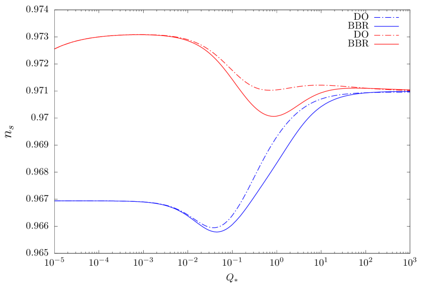
(a) $\Upsilon\propto\phi^{2}$

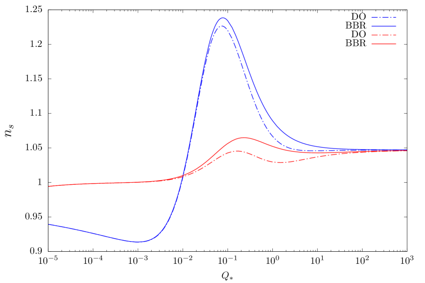
(b) $\Upsilon\propto T^{3}/\phi^{2}$

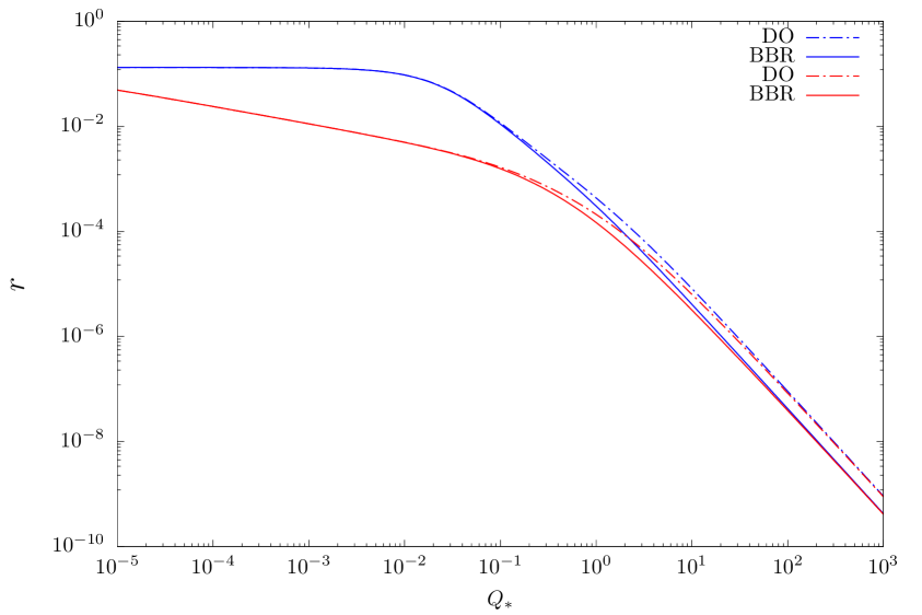
(c) $\Upsilon\propto\phi^{2}$

(d) $\Upsilon\propto T^{3}/\phi^{2}$

Figure 1: Predictions for a quadratic potential considering $60$ e-folds of expansion. Shown are at the top the spectral index and at the bottom the tensor-to-scalar ratio. Red lines denote $n_{*}=n_{BE}$ and blue lines $n_{*}=0$.

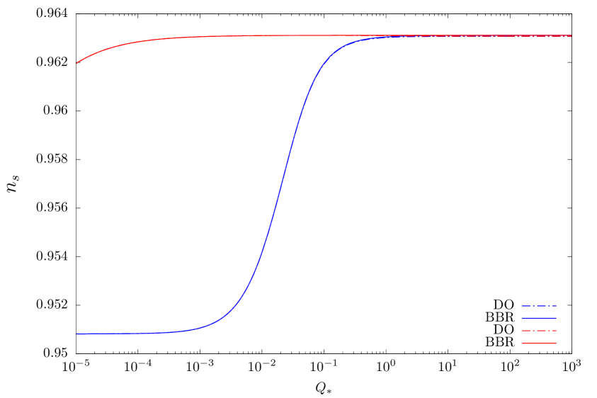
(a) $\Upsilon\propto\phi^{2}$

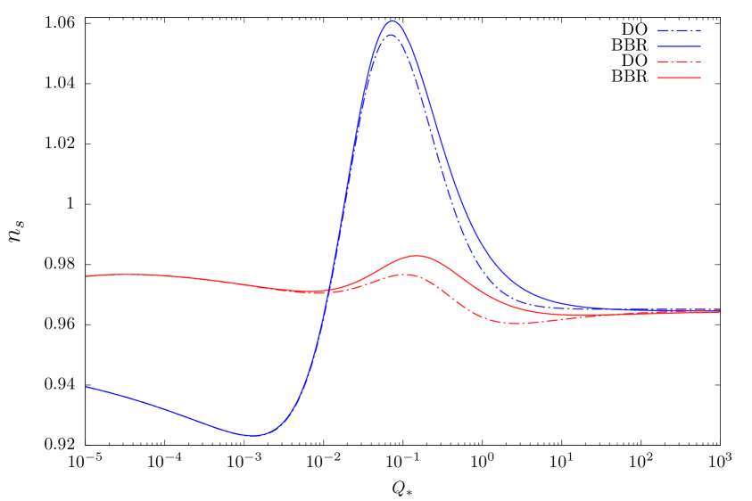
(b) $\Upsilon\propto T^{3}/\phi^{2}$

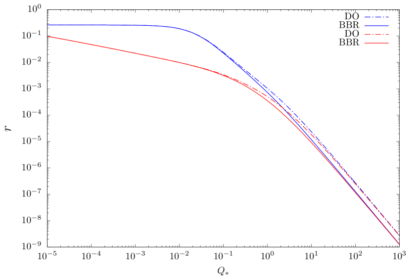
(c) $\Upsilon\propto\phi^{2}$

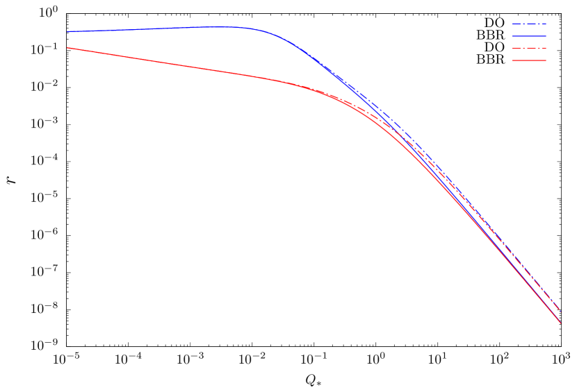
(d) $\Upsilon\propto T^{3}/\phi^{2}$

Figure 2: Predictions for a quartic potential considering $60$ e-folds of expansion. Shown are at the top the spectral index and at the bottom the tensor-to-scalar ratio. Red lines denote $n_{*}=n_{BE}$ and blue lines $n_{*}=0$.

The hybrid potentials are also examined, with results shown in Fig. 3. This potential has two scalar fields, although during slow-roll inflation only the inflaton degrees of freedom are excited. Then, most of inflation takes place until $\phi$ gets to a critical value $\phi_{c}$, where the so-called waterfall field is relevant for the background dynamics, bringing inflation to its end soon after that. Therefore, during slow-roll, we can set the waterfall field to zero and write the potential as

$$V(\phi)=V_{0}\left(1+\frac{k}{2}\phi^{2}\right).$$ (4.38)

As a way to impose a condition on $k$, we required $\eta(\phi_{c})=0.1$. Since this does not fix all the required degrees of freedom, a condition on $\phi_{c}$ is also imposed. For quadratic dissipation, $\phi_{c}=0.1$ was taken, whereas for $\Upsilon\propto T^{3}/\phi^{2}$ it was $\phi_{c}=0.0045$, since it was complicated to get 60 e-folds of expansion with higher values. Anyway, the same qualitative behaviour was found, i.e., bigger differences in the spectral index when dissipation and expansion occur at similar rates.

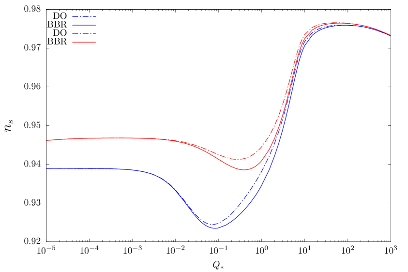
(a) $\Upsilon\propto\phi^{2}$

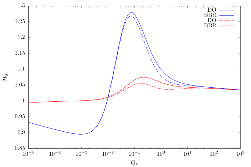
(b) $\Upsilon\propto T^{3}/\phi^{2}$

(c) $\Upsilon\propto\phi^{2}$

(d) $\Upsilon\propto T^{3}/\phi^{2}$

Figure 3: Predictions for a hybrid potential considering $60$ e-folds of expansion. Shown are at the top the spectral index and at the bottom the tensor-to-scalar ratio. Red lines denote $n_{*}=n_{BE}$ and blue lines $n_{*}=0$.

5 Discussion

In this article we have reexamined the two existing analytical approaches to compute the comoving curvature perturbation and the observables derived from it within the WI scenario. This is the first such explicit comparison between them, perhaps because one would expect the results to agree due to a number of reasons including the gauge invariant nature of General Relativity. However, the formulas for the amplitude of the primordial spectrum differ, with a “$Q/4$-difference” spoiling the equivalence at leading order. This has consequences especially for the spectral index, with differences in the predicted values of order $\mathcal{O}(10^{-3})$ in dissipative regions where $Q\sim 1$; this was shown both analytically and in specific realisations.

The origin of the discrepancies was found to be the different approximations performed in each approach. On the one hand, DO considers the time variation of the velocity field to be negligible, whereas BBR does so with the radiation momentum perturbation. Each assumption leads to different results because part of the dilution of the momentum perturbation is encompassed in the time variation of the velocity field. Given the dependence of $\mathcal{R}$ on $\Psi$, we conclude that the BBR approximation is a more sensible one, otherwise one would be underestimating the damping effect of expansion on the momentum perturbation, and consequently, on the curvature perturbation and the observables depending directly on that magnitude. Once this point is recognized, both methodologies are consistent at leading order. This is explained by the fact that both approaches considered the slow-roll approximation to be also valid for perturbed quantities. In Appendix D, we explicitly show through numerical simulations that this is a well-founded assumption, in particular for the momentum perturbation. In this way, we are entitled to ignore the higher order time derivatives in the equations of motion of perturbations. Other terms that are consistently neglected at leading order are the metric and source perturbations, as well as the coupling between radiation and the metric perturbations. However, we do account for those terms in Appendix C, where we follow the same program as before, obtaining an expression for the curvature perturbation valid at next-to-leading order. We found that there are no corrections to $\mathcal{R}$ at that order, since the total gauge invariant momentum perturbation and $\rho+p$ change by the same factor.

Appendix A Slow-roll parameter $\theta$

In order to derive the slow-roll parameter $\theta$ for a general $T$-dependent dissipative coefficient, $\Upsilon\propto T^{c}/\phi^{m}$, the evolution of the temperature in the slow-roll regime is needed. Using the Stefan-Boltzmann law together with the slow-roll equation for $\rho_{r}$ gives

$$\rho_{r}=C_{r}T^{4}\simeq\frac{3}{4}Q\dot{\phi}^{2},$$ (A.1)

which leads to

$$\frac{d\ln T}{dN} = \frac{1}{2}(\epsilon-\eta)+\frac{1-Q}{4Q}\theta\,.$$ (A.2)

Therefore,

$$\frac{d\ln\Upsilon}{dN} = c\frac{d\ln T}{dN}-m\frac{d\ln\phi}{dN}$$ (A.3)

$$= c\left[\frac{1}{2}(\epsilon-\eta)+\frac{1-Q}{4Q}\theta\right]+m\sigma\,,$$ (A.4)

and thus,

$$\theta=\frac{Q}{1+Q}\frac{d\ln Q}{dN}=\frac{4Q}{4-c+(4+c)Q}\left[\left(1+\frac{c}{2}\right)\epsilon-\frac{c}{2}\eta+m\sigma\right]\,.$$ (A.5)

In particular for a monomial dissipative coefficient $\Upsilon\propto\phi^{n}$, setting $c=0$ and $m=-n$ in (A.5) gives,

$$\theta=\frac{Q}{1+Q}(\epsilon-n\sigma)\,.$$ (A.6)

Appendix B Approach-Independent part of the Spectral Index

In this section a derivation is outlined for an analytical expression for $\tilde{n}$,

$$\tilde{n}=\frac{d}{dN}\ln\left[\left(\frac{\dot{\phi}}{2m_{P}^{2}\epsilon H}\right)^{2}\Delta^{2}_{\delta\phi}\right]\,,$$ (B.1)

which as introduced in (4.28), is independent of the approach to compute the comoving curvature perturbation and its corresponding power spectrum. The inflaton power spectrum is given by:

$$\Delta^{2}_{\delta\phi}=\left(\frac{H}{2\pi}\right)^{2}(1+2n_{*}+\frac{T}{H}F[Q])\,,$$ (B.2)

where

$$F[Q]=\frac{12Q8^{Q}[\Gamma(3/2+3Q/2)]^{3}}{(1+3Q)\Gamma(1+3Q/2)\Gamma(5/2+3Q)}\,,$$ (B.3)

and either $1+2n_{*}\simeq 1$, or $1+2n_{*}\simeq 2T/H$ for the Bose-Einstein distribution. Therefore, in general, $\tilde{n}$ is given by

$$\tilde{n}=2\eta-6\epsilon+\frac{d\ln(1+n_{*}+(T/H)F[Q])}{dN}\,,$$ (B.4)

where (2.9) and (2.10) are used, together with (2.11) in order to compute the derivative of the slow-roll parameter $\epsilon$. On the other hand, the last term on the RHS is model dependent. For instance, consider the case with $n_{*}=0$, so that

$$\frac{d\ln(1+(T/H)F[Q])}{dN} = \frac{(T/H)F[Q]}{1+(T/H)F[Q]}\left[\frac{1}{4}(6\epsilon-2\eta)+\left(\frac{1-Q}{4Q}+\frac{1+Q}{Q}F^{\prime}[Q]\right)\theta\right]\,,$$ (B.5)

where we have defined $F^{\prime}[Q]=d\ln F[Q]/d\ln Q$, and we have used (A.2) and (A.5) together with the definition of $\epsilon$. Collecting all the terms gives for $\tilde{n}$,

$$\tilde{n}=\left(1-\frac{(T/H)F[Q]}{1+(T/H)F[Q]}\right)(2\eta-6\epsilon)+\frac{(T/H)F[Q]}{1+(T/H)F[Q]}\left(\frac{1-Q}{4Q}+\frac{1+Q}{Q}F^{\prime}[Q]\right)\theta\,.$$ (B.6)

This expression can be simplified in the weak (WDR) and strong (SDR) dissipative limits. For the former, the dissipative ratio satisfies $Q\ll 1$, which gives

$$\tilde{n}\simeq\left(1-\frac{\pi}{2}\frac{T}{H}Q\right)(2\eta-6\epsilon)+\frac{5\pi}{2}\frac{T}{H}\theta\,,$$ (B.7)

whereas for strong dissipation

$$\tilde{n}\simeq\left(\frac{3}{4}-\frac{1}{4}\frac{H/T}{\sqrt{3\pi Q}}\right)(2\eta-6\epsilon)+\left(1-\frac{H/T}{\sqrt{3\pi Q}}\right)\frac{\theta}{4}\,.$$ (B.8)

A similar procedure can be followed for the case $n_{*}=n_{BE}$, where the expression for $\tilde{n}$ now reads

$$\tilde{n}=\frac{3}{4}(2\eta-6\epsilon)+\frac{1-Q}{4Q}\theta+\frac{F[Q]}{2+F[Q]}F^{\prime}[Q]\frac{1+Q}{Q}\theta\,.$$ (B.9)

Taking again the limits for weak and strong dissipation, gives for $Q\ll 1$,

$$\tilde{n}\simeq\frac{3}{4}(2\eta-6\epsilon)+\left(\frac{1}{4Q}+\pi-\frac{1}{4}\right)\theta\,,$$ (B.10)

whereas for $Q\gg 1$ it reads,

$$\tilde{n}\simeq\frac{3}{4}(2\eta-6\epsilon)+\left(\frac{1}{4}-\frac{1}{\sqrt{3\pi Q}}\right)\theta\,.$$ (B.11)

Appendix C Corrections to the comoving curvature perturbation at linear order

In this section, we intend to derive a formula for the comoving curvature perturbation, including corrections at higher order, if any. In doing so, some gaps in the derivation obtained at zeroth order in Section 4.2 are filled. There are two central parts in the derivation, which we can identify by looking at the definition of the comoving curvature perturbation,

$$\mathcal{R}=-\frac{H}{\rho+p}\Psi_{T}^{GI}=-\frac{H}{\rho+p}\left(\Psi_{\phi}^{GI}+\Psi_{r}^{GI}\right).$$ (C.1)

Clearly, both the numerator (through $\Psi_{r}^{GI}$) and the denominator (through $\rho_{r}$) require “improved” expressions in order to get one for $\mathcal{R}$. To get such formulas, the plan in both cases is to solve perturbatively the corresponding equations, using the slow-roll approximation when appropriate.

C.1 Corrections to $\rho_{r}$

First, we will compute the corrections for the denominator of (C.1), given by

$$\rho+p=\dot{\phi}^{2}+\frac{4}{3}\rho_{r}.$$ (C.2)

Since the higher order terms come from the radiation energy density, henceforth we will focus on this variable. At zeroth order, it satisfies

$$\rho_{r}^{(0)}\simeq\frac{3}{4}Q\dot{\phi}^{2},$$ (C.3)

which no longer holds at the desired level of approximation. To solve this, we posit that it can be written as a series in the slow-roll parameter $\epsilon$ like

$$\rho_{r}=c_{0}+c_{1}\epsilon+\mathcal{O}(\epsilon^{2}).$$ (C.4)

Naturally, the first term corresponds to the usual slow-roll approximation, i.e., $\rho_{r}^{(0)}=c_{0}$. The second coefficient can be found by replacing this into the equation of motion of the radiation energy density (2.5), such that

$$\dot{c_{0}}+\dot{c_{1}}\epsilon+c_{1}\dot{\epsilon}+4H(c_{0}+c_{1}\epsilon)=\Upsilon\dot{\phi}^{2}=4Hc_{0},$$ (C.5)

where the second and third term on the LHS clearly introduce corrections at higher order. In consequence, the second coefficient is given by

$$c_{1}=-\frac{\dot{c_{0}}}{H\epsilon}=-\frac{\rho_{r}^{(0)}}{4\epsilon}\left(2(\epsilon-\eta)+\frac{1-Q}{Q}\theta\right),$$ (C.6)

so the radiation energy density now reads

$$\rho_{r}\simeq\rho_{r}^{(1)}=\frac{3}{4}Q\dot{\phi}^{2}\left(1-\frac{\epsilon-\eta}{2}-\frac{1-Q}{4Q}\theta\right).$$ (C.7)

As such, (C.2) becomes

$$\rho+p\simeq\dot{\phi}^{2}\left\{1+Q\left(1-\frac{\epsilon-\eta}{2}-\frac{1-Q}{4Q}\theta\right)\right\}\;.$$ (C.8)

C.2 Corrections to $\Psi_{r}$

In order to simplify the notation, we drop the superindex “GI” from the perturbations, but all of them should be understood to be in their gauge invariant form. Having said that, we write $\Psi_{r}$ in terms of its contributions at each order of approximation, i.e.,

$$\Psi_{r}\simeq\Psi_{r}^{(0)}+\Psi_{r}^{(1)},$$ (C.9)

where $\Psi_{r}^{(0)}=Q\Psi_{\phi}$, as shown in Section 4.2. In this way, the equation of motion of the momentum perturbation (3.16) becomes

$$\dot{\Psi}_{r}^{(0)}+3H\left(\Psi_{r}^{(0)}+\Psi_{r}^{(1)}\right)\simeq\Upsilon\Psi_{\phi}-\frac{1}{3}\rho_{r}-\frac{4}{3}\rho_{r}\mathcal{A},$$ (C.10)

where we have omitted $\dot{\Psi}_{r}^{(1)}$, as it is a higher order term. Then, the correction to the radiation momentum perturbation is given by

$$\Psi_{r}^{(1)}=-\frac{1}{9H}\left[\delta\rho_{r}+4\rho_{r}\mathcal{A}\right]-\frac{\dot{\Psi}_{r}^{(0)}}{3H}.$$ (C.11)

In order to continue, we need to invoke the other equations of motion, in particular (3.14) and (3.15). In both cases, we will use the slow-roll approximation, neglecting the higher time derivatives of each variable, which leads to the following equations

$$3H(1+Q)\dot{\delta\phi}+V_{\phi\phi}\delta\phi\simeq-\dot{\phi}\delta\Upsilon+\Upsilon\dot{\phi}\mathcal{A}+6H\dot{\phi}\mathcal{A},$$ (C.12)

$$4H\delta\rho_{r}\simeq\delta\mathcal{Q}_{r}+\mathcal{Q}_{r}\mathcal{A},$$ (C.13)

where we have also taken the $k\ll aH$ limit. From the first equation and the definition of the slow-roll parameter $\eta$, we can get the useful relation

$$\frac{\dot{\delta\phi}}{\dot{\phi}}\simeq-\frac{H}{\dot{\phi}}\eta\delta\phi-\frac{Q}{1+Q}\frac{\delta\Upsilon}{\Upsilon}+\frac{2+Q}{1+Q}\mathcal{A}.$$ (C.14)

Next, we will concentrate on getting an expression for $\delta\rho_{r}$. With this goal in mind, take the definition of the source, $\mathcal{Q}_{r}=\Upsilon\dot{\phi}^{2}$, such that its perturbation reads

$$\frac{\delta\mathcal{Q}_{r}}{\mathcal{Q}_{r}}=\frac{\delta\Upsilon}{\Upsilon}+2\left(\frac{\dot{\delta\phi}}{\dot{\phi}}-\mathcal{A}\right).$$ (C.15)

Furthermore, since $\Upsilon\propto T^{c}/\phi^{m}$ and $\rho_{r}\propto T^{4}$, we have that

$$\frac{\delta\Upsilon}{\Upsilon}=c\frac{\delta T}{T}-m\frac{\delta\phi}{\phi}=\frac{c}{4}\frac{\delta\rho_{r}}{\rho_{r}}-m\frac{\delta\phi}{\phi}.$$ (C.16)

Then, plugging (C.15) into (C.13), and using (C.14) and (C.16), we get

$$\frac{\delta\rho_{r}}{9H}=\frac{1+Q}{4-c+(4+c)Q}\frac{\dot{\phi}^{2}}{3H}Q\left[\frac{3+Q}{1+Q}\mathcal{A}-m\frac{1-Q}{1+Q}\frac{\delta\phi}{\phi}-2\frac{H}{\dot{\phi}}\eta\delta\phi\right].$$ (C.17)

Turning our attention back to (C.11), we need to compute the time derivative of the radiation momentum perturbation at zeroth order. Clearly, this is given by

$$\dot{\Psi}_{r}^{(0)}=\left(\dot{Q}\Psi_{\phi}+Q\dot{\Psi}_{\phi}\right),$$ (C.18)

where

$$\dot{Q}=H(1+Q)\theta,$$ (C.19)

$$\dot{\Psi}_{\phi}=-(\ddot{\phi}\delta\phi+\dot{\phi}\dot{\delta\phi}).$$ (C.20)

We can conveniently write $\ddot{\phi}$ in terms of the slow-roll parameters through (2.9), which yields

$$\ddot{\phi}\simeq H(\epsilon-\eta-\theta)\dot{\phi}.$$ (C.21)

Then, invoking (C.14) once again, the time derivative of the field momentum perturbation reads

$$\dot{\Psi}_{\phi}=H(\epsilon-2\eta-\theta)\Psi_{\phi}+\dot{\phi}^{2}\left\{\frac{Q}{1+Q}\left[\frac{c}{4}\frac{\delta\rho_{r}}{\rho_{r}}-m\frac{\delta\phi}{\phi}\right]-\frac{2+Q}{1+Q}\mathcal{A}\right\},$$ (C.22)

and, consequently, (C.18) becomes

$$\dot{\Psi}_{r}^{(0)}=H\theta\Psi_{\phi}+Q\left[H(\epsilon-2\eta)\Psi_{\phi}+\dot{\phi}^{2}\left\{\frac{Q}{1+Q}\left[\frac{c}{4}\frac{\delta\rho_{r}}{\rho_{r}}-m\frac{\delta\phi}{\phi}\right]-\frac{2+Q}{1+Q}\mathcal{A}\right\}\right],$$ (C.23)

where, in addition, we have used (C.19). Hence, plugging this into (C.11) and rearranging similar terms, we get

$$\Psi_{r}^{(1)}=-\frac{1+(1+c)Q}{1+Q}\frac{\delta\rho_{r}}{9H}+\frac{\dot{\phi}^{2}}{3H}\frac{Q}{1+Q}\mathcal{A}-\frac{Q}{3}\left(\epsilon-2\eta+\frac{\theta}{Q}\right)\Psi_{\phi}+\frac{\dot{\phi}^{2}}{3H}\frac{mQ^{2}}{1+Q}\frac{\delta\phi}{\phi}.$$ (C.24)

Replacing (C.17) above, it follows that

$$\Psi_{r}^{(1)} = \frac{\dot{\phi}^{2}}{3H}\frac{mQ}{1+Q}\frac{\delta\phi}{\phi}\left[Q+\frac{1+(1+c)Q}{4-c+(4+c)Q}(1-Q)\right]+\frac{2}{3}Q\eta\Psi_{\phi}\left[1-\frac{1+(1+c)Q}{4-c+(4+c)Q}\right]$$ (C.25)

$$+\frac{\dot{\phi}^{2}}{3H}\frac{Q}{1+Q}\mathcal{A}\left[1-\frac{1+(1+c)Q}{4-c+(4+c)Q}(3+Q)\right]-\left[Q\frac{\epsilon}{3}+\frac{\theta}{3}\right]\Psi_{\phi}\;.$$

The remaining task is to write the terms proportional to $\delta\phi/\phi$ and $\mathcal{A}$ as functions of $\Psi_{\phi}$. The former can be easily done by considering the slow-roll parameter $\sigma$ together with (A.5), which yields

$$\sigma=-\frac{d\ln\phi}{dN}=-\frac{\dot{\phi}}{H\phi}=\frac{1}{m}\left[-\left(1+\frac{c}{2}\right)\epsilon+\frac{c}{2}\eta+\frac{4-c+(4+c)Q}{4Q}\theta\right].$$ (C.26)

Finally, the term proportional to $\mathcal{A}$ can be easily dealt with by noticing that

$$\mathcal{A}=\epsilon\mathcal{R}=\epsilon(\mathcal{R}^{(0)}+\mathcal{R}^{(1)}),$$ (C.27)

where, as usual, the second term on the RHS introduces higher order corrections (and which we are trying to compute). Thus, at this stage, it will be enough to keep the first term, such that

$$\mathcal{A}^{(0)}=\epsilon\mathcal{R}^{(0)}=-\frac{\epsilon H}{\dot{\phi}^{2}}\Psi_{\phi}.$$ (C.28)

Therefore, replacing (C.26) and (C.28) in (C.25), and after some algebra, we have got that

$$\Psi_{r}^{(1)}=Q\left(-\frac{\epsilon}{2}+\frac{\eta}{2}-\frac{1-Q}{4Q}\theta\right)\Psi_{\phi},$$ (C.29)

and, thus, the radiation momentum perturbation at next-to-leading order is

$$\Psi_{r}=Q\left(1-\frac{\epsilon}{2}+\frac{\eta}{2}-\frac{1-Q}{4Q}\theta\right)\Psi_{\phi}.$$ (C.30)

Notice that the total momentum perturbation now reads

$$\Psi_{T}=\left\{1+Q\left(1-\frac{\epsilon-\eta}{2}-\frac{1-Q}{4Q}\theta\right)\right\}\Psi_{\phi},$$ (C.31)

i.e., it has the same correction factor as the one we found for $\rho+p$. In consequence, they cancel each other out in (C.1), so that

$$\mathcal{R}=-\frac{H}{\dot{\phi}^{2}}\left[1+\mathcal{O}(\epsilon^{2})\right]\Psi_{\phi}.$$ (C.32)

Appendix D Ratio between $\dot{\Psi}_{r}$ and $H\Psi_{r}$

As a way of expanding on the argument about the discrepancies between DO and BBR, and the validity of the slow-roll approximation for perturbed variables, we present in Fig. 4 the result of numerical simulations showing the ratio between $d\Psi_{r}/dN$ and $\Psi_{r}$ for a quartic potential and two types of dissipative coefficients, $\Upsilon\propto\phi^{2}$ (left) and $\Upsilon\propto T^{3}/\phi^{2}$ (right). The slow-roll parameter $\epsilon\equiv\epsilon_{H}$ is shown as a reference. Thus, in the first case, it can be seen that the ratio is of order $\mathcal{O}(\epsilon^{2})$, whereas for the $T-$dependent one, it is of order $\mathcal{O}(\epsilon)$. In either case, at least for a leading order approximation, $\dot{\Psi}_{r}$ can be safely assumed to be negligible in comparison to $H\Psi_{r}$. In this way, the time derivative of the velocity field, given by

$$\dot{v}=\frac{3}{4}\frac{k}{a\rho_{r}}\left(\dot{\Psi}_{r}-\frac{\dot{\rho}_{r}}{\rho_{r}}\Psi_{r}-H\Psi_{r}\right),$$ (D.1)

can be well approximated by

$$\dot{v}\simeq-\frac{3}{4}\frac{k}{a}\frac{H}{\rho_{r}}\Psi_{r}.$$ (D.2)

However, it is worth emphasizing that this is not negligible at a leading-order approximation, as discussed in Section 4.3, because it encompasses part of the dilution of the radiation momentum perturbation.

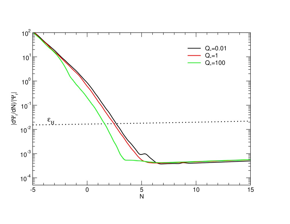
(a) $\Upsilon\propto\phi^{2}$

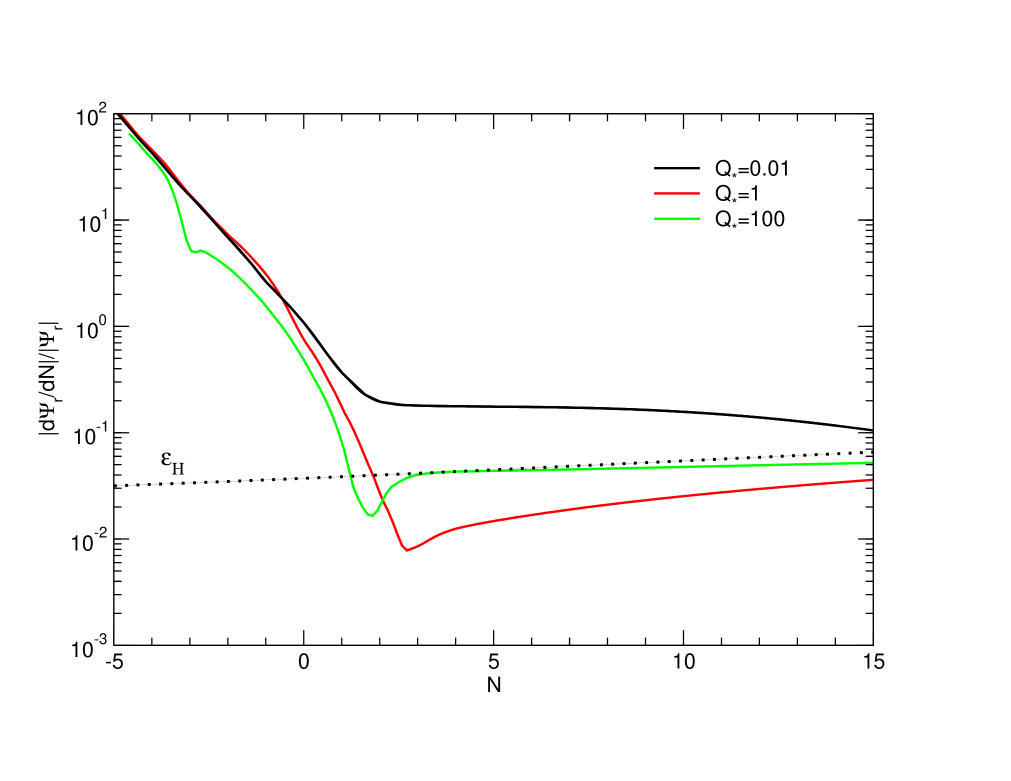
(b) $\Upsilon\propto T^{3}/\phi^{2}$

Figure 4: Ratio between $d\Psi_{r}/dN$ and $\Psi_{r}$ or, equivalently, $\dot{\Psi}_{r}$ and $H\Psi_{r}$, for a quartic potential. The dotted line shows the evolution of the slow-roll parameter $\epsilon\equiv\epsilon_{H}$ with $N$. The figures are plotted such that $k=aH$ at $N=0$, and the end of inflation happens at $N=60$.

References

- [1] A. H. Guth, Inflationary universe: A possible solution to the horizon and flatness problems, Phys. Rev. D 23 (1981) 347.
- [2] A. Linde, A new inflationary universe scenario: A possible solution of the horizon, flatness, homogeneity, isotropy and primordial monopole problems, Phys. Lett. B 108 (1982) 389 .
- [3] A. Linde, Scalar field fluctuations in the expanding universe and the new inflationary universe scenario, Phy. Lett. B 116 (1982) 335 .
- [4] A. Albrecht and P. J. Steinhardt, Cosmology for grand unified theories with radiatively induced symmetry breaking, Phys. Rev. Lett. 48 (1982) 1220.
- [5] É. B. Gliner and I. G. Dymnikova, A nonsingular Friedmann cosmology, Pisma Astron. Zh. 01 (1975) 7.
- [6] R. Brout, F. Englert and E. Gunzig, The creation of the universe as a quantum phenomenon, Annals Phys. 115 (1978) 78 .
- [7] R. Brout, F. Englert and E. Gunzig, The causal universe, Gen. Rel. Grav. 10 (1979) 1.
- [8] A. Starobinsky, A new type of isotropic cosmological models without singularity, Phys. Lett. B 91 (1980) 99 .
- [9] L. Fang, Entropy generation in the early universe by dissipative processes near the higgs phase transition, Phys. Lett. B 95 (1980) 154 .
- [10] D. Kazanas, Dynamics of the universe and spontaneous symmetry breaking, Astrophys. J. 241 (1980) L59.
- [11] E. W. Kolb and S. Wolfram, Spontaneous symmetry breaking and the expansion rate of the early universe, Astrophys. J. 239 (1980) 428.
- [12] A. Berera, Warm inflation, Phys. Rev. Lett. 75 (1995) 3218 [9509049].
- [13] M. Bastero-Gil and A. Berera, Warm Inflation Model Building, Int. J. Mod. Phys. A 24 (2009) 2207.
- [14] A. Berera, Warm inflation in the adiabatic regime — a model, an existence proof for inflationary dynamics in quantum field theory, Nucl. Phys. B 585 (2000) 666 .
- [15] M. Bastero-Gil, A. Berera, R. Hernández-Jiménez and J. G. Rosa, Warm inflation within a supersymmetric distributed mass model, 1801.02648.
- [16] H. P. De Oliveira, Density perturbations in warm inflation and COBE normalization, Phys. Lett. B 526 (2002) 1 [0202045v1].
- [17] S. Del Campo, R. Herrera and D. Pavón, Cosmological perturbations in warm inflationary models with viscous pressure, Phys. Rev. D 75 (2007) 083518 [0703604v1].
- [18] R. O. Ramos and L. A. Da Silva, Power spectrum for inflation models with quantum and thermal noises, JCAP 03 (2013) 032 [1302.3544].
- [19] M. Bastero-Gil, A. Berera and R. O. Ramos, Shear viscous effects on the primordial power spectrum from warm inflation, JCAP 1107 (2011) 030 [1106.0701].
- [20] A. R. Liddle, P. Parsons and J. D. Barrow, Formalizing the slow-roll approximation in inflation, Phys. Rev. D 50 (1994) 7222.
- [21] P. Adshead, R. Easther, J. Pritchard and A. Loeb, Inflation and the Scale Dependent Spectral Index: Prospects and Strategies, JCAP 1102 (2011) 021 [1007.3748].
- [22] Planck collaboration, Planck 2015 results. XIII. Cosmological parameters, Astron. Astrophys. 594 (2016) A13 [1502.01589].
- [23] R. Rangarajan, Current Status of Warm Inflation, 1801.02648.
- [24] J.-C. Hwang, Perturbations of the Robertson-Walker space - Multicomponent sources and generalized gravity, Astrophys. J. (1991) .
- [25] D. Baumann, TASI Lectures on Inflation, 0907.5424.
- [26] L. M. H. Hall, I. G. Moss and A. Berera, Scalar perturbation spectra from warm inflation, Phys. Rev. D 69 (2004) 083525.
- [27] C. Graham and I. G. Moss, Density fluctuations from warm inflation, JCAP 0907 (2009) 013 [0905.3500].
- [28] A. Berera and L.-Z. Fang, Thermally induced density perturbations in the inflation era, Phys. Rev. Lett. 74 (1995) 1912.
- [29] K. A. Malik, D. Wands and C. Ungarelli, Large-scale curvature and entropy perturbations for multiple interacting fluids, Phys. Rev. D 67 (2003) 063516.
- [30] S. Bartrum, M. Bastero-Gil, A. Berera, R. Cerezo, R. O. Ramos and J. G. Rosa, The importance of being warm (during inflation), Phys. Lett. B 732 (2014) 116 [arXiv:1307.5868v1].
- [31] M. Bastero-Gil, A. Berera, R. O. Ramos and J. G. Rosa, Warm Little Inflaton, Phys. Rev. Lett. 117 (2016) 151301 [1604.08838].
- [32] M. Benetti and R. O. Ramos, Warm inflation dissipative effects: predictions and constraints from the Planck data, Phys. Rev. D 95 (2017) 023517 [1610.08758].
- [33] M. Bastero-Gil, S. Bhattacharya, K. Dutta and M. R. Gangopadhyay, Constraining Warm Inflation with CMB data, JCAP 1802 (2018) 054 [1710.10008].
- [34] R. Arya and R. Rangarajan, Study of warm inflationary models and their parameter estimation from CMB, 1812.03107.
- [35] R. Arya, A. Dasgupta, G. Goswami, J. Prasad and R. Rangarajan, Revisiting CMB constraints on warm inflation, JCAP 1802 (2018) 043 [1710.11109].
- [36] A. N. Taylor and A. Berera, Perturbation spectra in the warm inflationary scenario, Phys. Rev. D 62 (2000) 083517 [astro-ph/0006077].