Describing phase transitions in field theory by self-similar approximants

Abstract

Self-similar approximation theory is shown to be a powerful tool for describing phase transitions in quantum field theory. Self-similar approximants present the extrapolation of asymptotic series in powers of small variables to the arbitrary values of the latter, including the variables tending to infinity. The approach is illustrated by considering three problems: (i) The influence of the coupling parameter strength on the critical temperature of the $O(N)$-symmetric multicomponent field theory. (ii) The calculation of critical exponents for the phase transition in the $O(N)$-symmetric field theory. (iii) The evaluation of deconfinement temperature in quantum chromodynamics. The results are in good agreement with the available numerical calculations, such as Monte Carlo simulations, Padé-Borel summation, and lattice data.

1 Introduction

Phase transitions in field theory are known to be a very interesting physical problem, whose description usually confronts complicated calculational challenges (see, e.g., Satz_1 ; Hagedorn_2 ; Cleymans_3 ; Reeves_4 ; Kleinert_5 ). Our aim in this report is to show that the description of phase transitions can be efficiently done by an original technique called self-similar approximation theory. This theory allows us to find analytical expressions for the sought solutions, it is rather simple, involving only low-cost calculations, and at the same time, it is very accurate, being comparable in accuracy with heavy numerical calculations.

The typical problem is that, as a rule, in the vicinity of a phase transition there are no small parameters, while calculations could be accomplished by means of perturbation theory in powers of such parameters, which leads to divergent series. There exist techniques allowing for effective summation of such series, for instance, Padé approximation Baker_6 or Borel summation Kleinert_5 . However, these techniques not always are applicable, as is discussed in Refs. Baker_7 ; Yukalov_8 ; Gluzman_9 ; Yukalov_10 .

Below we show that self-similar approximation theory overcomes the problems of asymptotic perturbation theory, making it possible to find analytic approximate solutions that are valid for the whole range of variables between zero to infinity. This theory combines simplicity with good accuracy.

The layout of the paper is as follows: In Sec. 2, we formulate the mathematical problem, giving the sketch of the main ideas the self-similar approximation theory is based on, and present two types of resulting approximants. In Sec. 3, we illustrate the use of the approach for studying the influence of the coupling parameter strength on the critical temperature of the $O(N)$-symmetric multicomponent field theory. Section 4 shows how the critical exponents for the phase transition in the $O(N)$-symmetric field theory can be calculated. And in Sec. 5, we demonstrate that, being based on weak-coupling high-temperature expansions, with employing self-similar approximation theory, it is possible to estimate the temperature of deconfinement phase transition in quantum chromodynamics. Section 6 summarizes the results.

2 Main ideas of self-similar approximation theory

Suppose we are looking for a physical quantity corresponding to a real function $f(x)$ satisfying very complicated equations that can be solved only by means of perturbation theory in powers of the asymptotically small real variable $x$, yielding

$$f(x)\simeq f_{k}(x)\qquad(x\rightarrow 0)\;,$$ (1)

with the $k$-th order series

$$f_{k}(x)=f_{0}(x)\left(1+\sum_{n=1}^{k}a_{n}x^{n}\right)\;,$$ (2)

where $f_{0}(x)$ is a given function. At the same time, our aim is to find the values of the solution $f(x)$ at finite $x$ or in some cases even at $x\rightarrow\infty$. This implies that we need to extrapolate the asymptotic series (2), derived for small $x\rightarrow 0$, to the whole domain of the variable $x\in[0,\infty)$. A general method of realizing such an extrapolation is provided by self-similar approximation theory Yukalov_11 ; Yukalov_12 ; Yukalov_13 ; Yukalov_14 ; Yukalov_15 , whose main ideas are as follows.

1. The sequence $\{f_{k}(x)\}$, with $k=1,2,\ldots$ has to be reorganized into another sequence $\{F_{k}(x,u_{k})\}$ by introducing parameters $u_{k}$ that are called control parameters because of their role in regulating the properties of the reorganized sequence $\{F_{k}(x,u_{k})\}$.

2. The control parameters $u_{k}$ are to be converted into control functions $u_{k}(x)$ such that to force the sequence $\{F_{k}(x,u_{k}(x))\}$ becoming convergent.

3. It is luring to discover a law, according to which a term $F_{k}$ transforms into $F_{k+1}$. If such a transformation law is known, then it would be straightforward to follow the chain of transformations $F_{k}\rightarrow F_{k+1}\rightarrow\ldots\rightarrow F^{*}$ leading to the sequence limit $F^{*}$ representing the sought function $f(x)$.

The introduction of control parameters can be done in several ways Yukalov_11 ; Yukalov_12 ; Yukalov_13 ; Yukalov_14 ; Yukalov_15 ; Yukalov_16 ; Yukalov_17 . For example, they can be introduced through initial conditions. Say, we are considering a system characterized by a Hamiltonian (or Lagrangian) $H$. We can take a simpler Hamiltonian $H_{0}(u)$ modeling the considered system and containing control parameters $u$. Introducing the Hamiltonian

$$H_{\varepsilon}=H_{0}(u)+\varepsilon[H-H_{0}(u)]\;,$$ (3)

one can resort to perturbation theory with respect to $\varepsilon$, calculating wave functions, or Green functions, or physical quantities

$$F_{k}(x,u_{k})=\langle\hat{A}(x)\rangle_{k}$$ (4)

related to some operators of observables, setting at the end $\varepsilon\rightarrow 1$.

The other way of introducing control parameters is by reexpansion tricks. Thus, when $f_{k}(x,m)$ in (2) depends on some parameter $m$, it is possible to make a substitution in (2), such as

$$m\longrightarrow u+\varepsilon(m-u)\;,\qquad x\longrightarrow\varepsilon x\;,$$

containing a control parameter $u$, and to reexpand the resulting $f_{k}(\varepsilon x,u+\varepsilon(m-u))$ in powers of $\varepsilon$, setting at the end $\varepsilon\rightarrow 1$.

Or one can incorporate a control parameter $u$ through a change of the variable $x=x(z,u)$ then reexpanding $f_{k}(x(z,u))$ in powers of $z$.

As an example of a change of the variable, it is possible to mention the conformal mapping

$$x=\frac{4u^{2}z}{(1-z)^{2}}\;,\qquad z=\frac{\sqrt{x+u^{2}}-u}{\sqrt{x+u^{2}}+u}\;.$$

One more method of introducing control parameters is by a functional transformation

$$\hat{T}[u_{k}]f_{k}(x)=F_{k}(x,u_{k})\;,\qquad f_{k}(x)=\hat{T}^{-1}[u_{k}]F_{k}(x,u_{k})\;,$$ (5)

containing these parameters.

One of the simplest transformations is given by the fractal transform

$$\hat{T}[u]f_{k}(x)=x^{u}f_{k}(x)$$ (6)

that is used for deriving self-similar approximants.

After control parameters are incorporated into the sequence, it is necessary to convert them into control functions governing the sequence convergence Yukalov_16 ; Yukalov_17 . The basic underlying idea is to connect the choice of control functions with the property of convergence that is expressed in the Cauchy criterion of convergence. The Cauchy criterion tells us that the sequence $\{F_{k}(x,u_{k})\}$ converges if and only if for each $\varepsilon>0$ there exists such $n_{\varepsilon}$ that

$$|\;F_{k+p}(x,u_{k+p})-F_{k}(x,u_{k})\;|<\varepsilon$$ (7)

for all $k>n_{\varepsilon}$ and $p\geq 0$.

The Cauchy criterion and the methods of optimal control theory suggest that, in order to induce fastest convergence, control functions have to minimize the fastest-convergence cost functional

$${\cal C}[u]=\sum_{k}|\;F_{k+p}(x,u_{k+p})-F_{k}(x,u_{k})\;|.$$ (8)

Thus control functions are defined as the minimizers of this cost functional,

$$\min_{u}{\cal C}[u]\rightarrow u_{k}(x)\;.$$ (9)

The practical methods of the minimization can be found in Refs. Yukalov_11 ; Yukalov_12 ; Yukalov_13 ; Yukalov_14 ; Yukalov_15 ; Yukalov_16 ; Yukalov_17 .

Substituting the found control functions into $F_{k}(x,u_{k})$ yields the optimized approximants

$$\widetilde{f}_{k}(x)=F_{k}(x,u_{k}(x))\;.$$ (10)

These approximants already can extrapolate the asymptotic series (2) to finite values of the variable $x$. But we want to go a step further, trying to find a transformation law between the terms $\widetilde{f}_{k}(x)$ and $\widetilde{f}_{k+1}(x)$, or more generally, a law transforming $\widetilde{f}_{k}(x)$ into $\widetilde{f}_{k+p}(x)$.

To derive a transformation law between $\widetilde{f}_{k}(x)$ and $\widetilde{f}_{k+p}(x)$, we can treat this transformation as a motion in the space of approximants, with the approximation order playing the role of discrete time. In other words, we need to construct a dynamical system describing this motion. The correct mathematical description of a dynamical system requires to formulate the motion in terms of endomorphisms Hirsch_18 ; Crutchfield_19 ; Cook_20 . For this purpose, we define the expansion function $x=x_{k}(f)$ given by the reonomic constraint

$$F_{0}(x,u_{k}(x))=f\;,\qquad x=x_{k}(f)\;.$$ (11)

And the required endomorphism takes the form

$$y_{k}(f)\equiv\widetilde{f}_{k}(x_{k}(f))\;.$$ (12)

By this construction, if the sequence of the approximants $\{\widetilde{f}_{k}(x)\}$, with increasing $k$, tends to a limit $\widetilde{f}(x)$, then the sequence of the endomorphisms $\{y_{k}(f)\}$ tends to a fixed point $y^{*}(f)$. In the vicinity of a fixed point, the endomorphism satisfies the self-similar relation

$$y_{k+p}(f)=y_{k}(y_{p}(f))\;.$$ (13)

Equation (13) describes the motion in the space of approximants with respect to the discrete time $k$ being the approximation order. A dynamical system in discrete time is called cascade. Since it describes the motion in the space of approximants, it is named approximation cascade. By construction, the trajectory of the approximation cascade $\{y_{k}(f)\}$ is bijective to the sequence of approximants $\{\widetilde{f}_{k}(x)\}$, so that the fixed point $y^{*}(f)$ is bijective to the sequence limit $\tilde{f}(x)$. In that way, to get the effective limit of the sought function, we need to find the fixed point of the approximation cascade.

Usually, it is more convenient to deal with the equations of motion in continuous time. To this end, it is possible to embed the approximation cascade into an approximation flow that is a dynamical system in continuous time. The embedding of the cascade into a flow,

$$\{y_{k}(f):\;k=0,1,2,\ldots\}\subset\{y(t,f):t\geq 0\}\;,$$ (14)

implies that the flow satisfies the same equation of motion

$$y(t+t^{\prime},f)=y(t,y(t^{\prime},f))\;,$$ (15)

and the flow trajectory passes through all the points of the cascade trajectory,

$$y(k,f)=y_{k}(f)\;.$$ (16)

Relation (15) can be rewritten as the differential Lie equation

$$\frac{\partial}{\partial t}\;y(t,f)=v(y(t,f))\;,$$ (17)

in which the velocity $v(y)$ is analogous to the Gell-Mann-Low function in renormalization group approach. Integrating the above equation gives the integral form

$$\int_{y_{k}}^{y_{k}^{*}}\frac{dy}{v(y)}=t_{k}\;,$$ (18)

which allows us, starting from a point $y_{k}(f)$, and moving during time $t_{k}$ with the velocity $v_{k}(y)$, to find the approximate fixed point $y_{k}^{*}(f)$. Hence, we can find the self-similar approximant $f_{k}^{*}(x)$ for the sought function.

Applying the procedure, described above, to the asymptotic expansion (2) it is possible to derive several forms of self-similar approximants. One is the self-similar factor approximant Yukalov_21 ; Gluzman_22 ; Yukalov_23

$$f_{k}^{*}(x)=f_{0}(x)\prod_{i=1}^{N_{k}}(1+A_{i}x)^{n_{i}}\;,$$ (19)

where

$$N_{k}=\left\{\begin{array}[]{ll}k/2\;,\nobreak\leavevmode&\leavevmode\nobreak\ k=2,4,\ldots\\ (k+1)/2\;,\nobreak\leavevmode&\leavevmode\nobreak\ k=3,5,\ldots\end{array}\right.\;.$$ (22)

This approximant provides the extrapolation of the asymptotic series (2), valid only for asymptotically small $x\rightarrow 0$, to the arbitrary values of the variable $x\in[0,\infty)$. All parameters $A_{i}$ and $n_{i}$, playing the role of control parameters, can be defined by the accuracy-through-order procedure comparing the asymptotic forms

$$f_{k}^{*}(x)\simeq f_{k}(x)\qquad(x\rightarrow 0)\;.$$ (23)

The other type of the approximants is the self-similar exponential approximant Yukalov_24

$$f_{k}^{*}(x)=f_{0}(x)\exp(C_{1}x\exp(C_{2}x\ldots\exp(C_{k}t_{k}x)))\;,$$ (24)

in which

$$C_{j}=\frac{a_{j}}{a_{j-1}}\qquad(j=1,2,\ldots,k)$$

and the control function $t_{k}=t_{k}(x)$ is defined by the equation

$$t_{k}=\exp(C_{k}xt_{k})\;.$$ (25)

The choice of the type of an approximant is dictated by the physics of the treated problem. When the considered physical quantities are expected to vary sufficiently slowly with the variation of $x$, one should use the factor approximants. And when one expects a fast variation of the physical quantities, exponential approximants are more appropriate.

3 Influence of coupling-parameter strength on critical temperature

As an application of the self-similar approximation theory, let us consider the second-order phase transition in the $O(N)$-symmetric field theory in three dimensions. The critical temperature depends on the coupling-parameter strength

$$\gamma\equiv\rho^{1/3}a_{s}\;,$$ (26)

where $\rho$ is average density and $a_{s}$, scattering length. For the free field theory, where $\gamma\rightarrow 0$, the critical temperature is

$$T_{0}=\frac{2\pi}{m}\left[\frac{\rho}{\zeta(3/2)}\right]^{2/3}\;.$$ (27)

The question is: how the critical temperature $T_{c}(\gamma)$ changes when the interaction is switched on?

One considers the relative critical temperature shift

$$\frac{\Delta T_{c}}{T_{0}}\equiv\frac{T_{c}(\gamma)-T_{0}}{T_{0}}\;.$$ (28)

At small $\gamma$, the shift behaves Baym_25 ; Baym_26 as

$$\frac{\Delta T_{c}}{T_{0}}\simeq c_{1}\gamma\qquad(\gamma\rightarrow 0)\;.$$ (29)

The coefficient $c_{1}$ can be calculated by using the loop expansion Kastening_27 ; Kastening_28 ; Kastening_29 resulting in the asymptotic series

$$c_{1}(x)\simeq\sum_{n=1}^{5}a_{n}x^{n}\qquad(x\rightarrow 0)$$ (30)

in powers of the variable

$$x=(N+2)\;\frac{\lambda}{\sqrt{\mu}}\;,$$

where $\lambda$ is a renormalized coupling and $\mu$, effective chemical potential. But the problem is that at the critical temperature, the chemical potential tends to zero, $\mu\rightarrow 0$.

Therefore the expansion variable tends to infinity, $x\rightarrow\infty$. So that to get $c_{1}$, we need to define $c_{1}(\infty)$, when expansion (30) becomes senseless. However in our approach, it is possible to define the effective limit $c_{1}(\infty)$ of expression (30) under $x\rightarrow\infty$.

Applying to the asymptotic series (30) our approach, we use self-similar factor approximants Yukalov_30 , as is explained in the previous section, getting for $c_{1}(x)$ the approximants

$$c_{1}(x)\rightarrow f_{k}^{*}(x)=a_{1}x\prod_{i=1}^{N_{k}}(1+A_{i}x)^{n_{i}}\;.$$ (31)

At large $x$, we have

$$f_{k}^{*}(x)\simeq B_{k}x^{\beta_{k}}\qquad(x\rightarrow\infty)\;,$$ (32)

where

$$B_{k}=a_{1}\prod_{i=1}^{N_{k}}A_{i}^{n_{i}}\;,\qquad\beta_{k}=1+\sum_{i=1}^{N_{k}}n_{i}\;.$$

The large-variable limit is finite, provided that $\beta_{k}=0$, which yields the value

$$f_{k}^{*}(\infty)=B_{k}\rightarrow c_{1}(\infty)$$ (33)

giving the sought coefficient $c_{1}$. The found coefficients $c_{1}$ for a different number of components $N$ in the $O(N)$-symmetric $\varphi^{4}$ field theory in $3d$ are shown in Table 1, where they are compared with available Monte Carlo simulations Kashurnikov_31 ; Arnold_32 ; Arnold_33 ; Sun_34 .

Table 1: The coefficient $c_{1}$ of the critical temperature shift, for a different number of the field components $N$, given by self-similar factor approximants, compared with the available Monte Carlo simulations.

$N$	$c_{1}$	Monte Carlo
0	0.77$\pm$ 0.03
1	1.06$\pm$ 0.05	1.09$\pm$ 0.09
2	1.29$\pm$ 0.07	1.29$\pm$ 0.05
		1.32$\pm$ 0.02
3	1.46$\pm$ 0.08
4	1.60$\pm$ 0.09	1.60$\pm$ 0.10

4 Calculation of critical exponents in $\varphi^{4}$ field theory

It is also possible to calculate critical exponents for the $O(N)$-symmetric $\varphi^{4}$ theory in $3d$ by applying self-similar approximation theory to the Wilson $\varepsilon$ expansions

$$f_{k}(\varepsilon)=\sum_{n=0}^{k}c_{n}\varepsilon^{n}\;,$$ (34)

where $\varepsilon=4-d$. Such expansions are derived for $\varepsilon\rightarrow 0$, while in reality $\varepsilon=1$.

The extrapolation of these asymptotic expansions can again be done by means of self-similar factor approximants

$$f_{k}^{*}(\varepsilon)=f_{0}(\varepsilon)\prod_{i=1}^{N_{k}}(1+A_{i}\varepsilon)^{n_{i}}\;.$$ (35)

Setting here $\varepsilon=1$, we define the answer as

$$f_{k}^{*}=\frac{1}{2}\;\left[f_{k}^{*}(1)+f_{k-1}^{*}(1)\right]\;,$$ (36)

with the error bar

$$\pm\;\frac{1}{2}\;\left[f_{k}^{*}(1)-f_{k-1}^{*}(1)\right]\;.$$

As an example, let us consider the $O(1)$ universality class for $3d$, which includes such a well known case as the three-dimensional Ising model. The $\varepsilon$-expansions for the critical exponents $\eta$, $\nu$, and $\omega$ have the form Kleinert_35 ; Kleinert_36

$$\eta\simeq 0.0185185\varepsilon^{2}+0.01869\varepsilon^{3}-0.00832877\varepsilon^{4}+0.0256565\varepsilon^{5}\;,$$

$$\nu^{-1}\simeq 2-0.333333\varepsilon-0.117284\varepsilon^{2}+0.124527\varepsilon^{3}-0.30685\varepsilon^{4}-0.95124\varepsilon^{5}\;,$$

$$\omega\simeq\varepsilon-0.62963\varepsilon^{2}+1.61822\varepsilon^{3}-5.23514\varepsilon^{4}+20.7498\varepsilon^{5}\;.$$ (37)

Other exponents can be found from the scaling relations

$$\alpha=2-3\nu\;,\qquad\beta=\frac{\nu}{2}\;(1+\eta)\;,\qquad\gamma=\nu(2-\eta)\;,\qquad\delta=\frac{5-\eta}{1+\eta}\;.$$ (38)

As is easy to check, the direct substitution of $\varepsilon=1$ in these expressions leads to bad results having little to do with the quantities that can be obtained in experiments or in numerical calculations. While extrapolating these expansions by means of self-similar factor approximants (35) and setting $\varepsilon=1$, we come to the values (36) that are close to those found in numerical calculations, such as the conformal bootstrap conjectureEl_37 ; El_38 ; Gliozzi_39 ; Komargodski_40 ; Kos_41 and Monte Carlo simulations Blote_42 ; Janke_43 ; Ferrenberg_44 ; Baillie_45 ; Holm_46 ; Holm_47 ; Chen_48 ; Holm_49 ; Li_50 ; Kanaya_51 ; Ballesteros_52 ; Caracciolo_53 ; Landau_54 ; Hasenbusch_55 ; Campostrini_56 ; Pelissetto_57 ; Deng_58 ; Hasenbusch_59 ; Campostrini_60 ; Hasenbusch_61 ; Ferrenberg_62 . Table 2 demonstrates the results obtained using the self-similar factor approximants, as compared with the numerical data of the conformal bootstrap conjecture, and Monte Carlo simulations.

Table 2: Critical exponents for $O(1)$-symmetric $\varphi^{4}$ field theory in $3d$, calculated using self-similar factor approximants (FA), conformal bootstrap conjecture (CB), and Monte Carlo simulations (MC).

	$FA$	$CB$	$MC$
$\alpha$	0.10645	0.11008	0.11026
$\beta$	0.32619	0.32642	0.32630
$\gamma$	1.24117	1.23708	1.23708
$\delta$	4.80502	4.78984	4.79091
$\eta$	0.03359	0.03630	0.03611
$\nu$	0.63118	0.62997	0.62991
$\omega$	0.78755	0.82966	0.830

We have also calculated the critical exponents for other $O(N)$-symmetric $\varphi^{4}$ theories, varying the number of components from $N=-2$ up to $N=10000$, and obtaining the values close to those derived by numerical methods, when these are available. It is important to stress that the critical exponents for $N=-2$ and $N\rightarrow\infty$ are known exactly and that in our approach we obtain the same exact values shown in Table 3.

Table 3: Exact critical exponents for $O(N)$-symmetric $\varphi^{4}$ field theory in $3d$ for $N=-2$ and $N=\infty$.

	$N=-2$	$N\rightarrow\infty$
$\alpha$	0.5	$-$1
$\beta$	0.25	0.5
$\gamma$	1	2
$\delta$	5	5
$\eta$	0	0
$\nu$	0.5	1
$\omega$	0.8	1

5 Estimation of deconfinement temperature in quantum chromodynamics

Self-similar approximation theory makes it possible to extrapolate asymptotic series at small variables to the whole domain of the latter. A very important question is whether it is feasible to predict the existence of a phase transition considering expansions very far from the transition point. Suppose we study the region of asymptotically weak coupling in QCD corresponding to high temperature. Is it possible to extract from such asymptotic expansions the information on the existence of the confinement-deconfinement phase transition? Below we show that extrapolating asymptotic series by self-similar approximants allows us to predict the deconfinement phase transition and to correctly estimate the transition temperature.

We consider the $SU(N_{c})$ QCD with three colours, $N_{c}=3$, and with massless quarks of $n_{f}$ flavors in the fundamental representation, with zero chemical potential. Using dimensional regularization and the modified minimal subtraction scheme $\overline{MS}$ one gets Zhai_63 ; Braaten_64 ; Kraemmer_65 the weak-coupling expansion of pressure in powers of the quantum chromodynamic coupling $\alpha_{s}$ or in powers of the coupling parameter $g$ connected by the relation

$$\alpha_{s}=\frac{g^{2}}{4\pi}\;.$$ (39)

This expansion reads as

$$P(g)\simeq\frac{8\pi^{2}}{45}\;T^{4}\;\left(\sum_{n=0}^{5}c_{n}g^{n}+c_{4}^{\prime}g^{4}\ln g\right)\;,$$ (40)

where $c_{1}=0$ and other coefficients can be found in Refs. Zhai_63 ; Braaten_64 ; Kraemmer_65 . In the Stefan-Boltzmann limit, one has

$$P_{0}\equiv P(0)=\frac{8\pi^{2}}{45}\;T^{4}\;\left(1+\frac{21}{32}\;n_{f}\right)\;.$$ (41)

It is convenient to define the relative pressure

$$p_{k}\equiv\frac{P_{k}}{P_{0}}=p_{k}(g,\mu,T)$$ (42)

that is a function of the coupling $g$, renormalization scale $\mu$, and temperature $T$, and where $P_{k}$ is the right-hand side of (40). Then we get

$$p_{k}=1+\sum_{n=2}^{5}\overline{c}_{n}g^{n}+\overline{c}_{4}^{\prime}g^{4}\ln g\;,$$ (43)

with $\overline{c}_{n}\equiv c_{n}/c_{0}$.

Defining the renormalization scale $\mu=\mu(g,T)$ from the minimal-difference condition Yukalov_66

$$p_{4}(g,\mu,T)-p_{3}(g,\mu,T)=0$$ (44)

reduces the relative pressure (43) to the form

$$p_{5}=1+\overline{c}_{2}g^{2}+\overline{c}_{3}g^{3}+\overline{c}_{5}g^{5}\;.$$ (45)

We extrapolate this expansion with the use of self-similar exponential approximants, as described in Sec. 2. Then we have the approximants to second order

$$p_{2}^{*}=\exp(C_{2}g^{2})\;,\qquad C_{2}=\frac{c_{2}}{c_{0}}\;,$$

to third order

$$p_{3}^{*}=\exp(C_{2}g^{2}t_{3})\;,$$

with

$$t_{3}=\exp(C_{3}gt_{3})\;,\qquad C_{3}=\frac{c_{3}}{c_{2}}\;,$$

and to fifth order

$$p_{5}^{*}=\exp(C_{2}g^{2}\exp(C_{3}gt_{5}))\;,$$ (46)

where

$$t_{5}=\exp(C_{5}g^{2}t_{5})\;,\qquad C_{5}=\frac{c_{5}}{c_{3}}\;.$$

The running coupling satisfies the renormalization group equation

$$\mu\;\frac{\partial g}{\partial\mu}=\beta(g)\;.$$ (47)

The Gell-Mann-Low function can be found Luthe_67 ; Baikov_68 in the weak-coupling limit

$$\beta(g)\simeq\beta_{k}(g)\qquad(g\rightarrow 0)$$

as a five-order expansion

$$\beta_{k}(g)=-\sum_{n=0}^{k}b_{n}g^{2n+3}=-b_{0}g^{3}\left(1+\sum_{n=1}^{k}\frac{b_{n}}{b_{0}}\;g^{2n}\right)\;,$$ (48)

with $k=5$ and the coefficients given in Ref. Luthe_67 ; Baikov_68 . As an initial condition for Eq. (47), we can take the value of the coupling for the $Z^{0}$ boson mass:

$$g(m_{Z})=1.22285\qquad(m_{Z}=91187\;{\rm Mev})\;.$$ (49)

The self-similar extrapolation of the Gell-Mann-Low function is

$$\beta_{k}^{*}(g)=-b_{0}g^{3}\exp\left(B_{1}g^{2}\exp\left(B_{2}g^{2}\ldots\exp\left(B_{k}t_{k}g^{2}\right)\right)\right)\;,$$ (50)

where

$$B_{j}=\frac{b_{j}}{b_{j-1}}\;,\qquad t_{k}=\exp\left(B_{k}g^{2}t_{k}\right)\;.$$

Solving the renormalization group equation (47), with the Gell-Mann-Low function (50) gives $g=g(\mu)$. Taking into account that the minimal-difference condition (44) defines $\mu=\mu(g,T)$, we find the temperature dependence for $g=g(T)$ and $\mu=\mu(T)$. Substituting this into pressure (46) gives the temperature dependence $p_{5}=p_{5}(T)$. The behavior of the latter for $n_{f}=6$ is shown in Fig. 1. With diminishing temperature from high values, the pressure, first, slightly deviates from the Stefan-Boltzmann limit and then sharply falls down to zero at $T_{c}\sim 150$ MeV. This temperature, representing the deconfinement phase transition, is in agreement with lattice data Borsanyi_69 ; Borsanyi_70 , as well as with some statistical models Yukalov_71 ; Yukalov_72 .

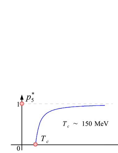
Figure 1: Behavior of temperature dependence $p_{5}=p_{5}(T)$ for $n_{f}=6$.

In this way, extrapolating high-temperature weak-coupling expansions by self-similar approximants shows the existence of deconfinement phase transition with a reasonable estimation of the deconfinement temperature of $T_{c}\sim 150$ MeV.

6 Conclusion

We have shown that self-similar approximation theory is a powerful tool for extrapolating asymptotic series in small variables to the whole region of the latter from zero to infinity. The application of the approach is illustrated by studying the influence of the coupling parameter strength in the $O(N)$-symmetric $\varphi^{4}$ theory on the critical temperature of symmetry breaking. The critical exponents for this phase transition are calculated. The results are in very good agreement with those of numerical methods, such as Monte Carlo simulations.

Also, we show that the approach makes it possible to predict the confinement-deconfinement phase transition in QCD by extrapolating high-temperature weak-coupling expansions. The predicted deconfinement temperature is in agreement with lattice calculations.

The important feature of the self-similar approximation theory is its simplicity, since it involves only low-cost calculations, as compared with numerical methods.

Note that the use of Padé approximants for this problem does not lead to reasonable results, exhibiting rather chaotic behavior with unphysical poles.

References

- (1) H. Satz, Phys. Rep. 88, 349 (1982).
- (2) R. Hagedorn, Riv. Nuovo Cimento 6, 1 (1983).
- (3) J. Cleymans, R. Gavai, and E. Suhonen, Phys. Rep. 130, 217 (1986).
- (4) [4] H. Reeves, Phys. Rep. 201, 335 (1991)
- (5) H. Kleinert, Path Integrals (World Scientific, Singapore, 2004).
- (6) G.A. Baker and P. Graves-Moris, Padé Approximants (Cambridge University, Cambridge, 1996).
- (7) G.A. Baker, Acta Appl. Math. 61, 37 (2000).
- (8) V.I. Yukalov, E.P. Yukalova, and S. Gluzman, J. Math. Chem. 47, 959–983 (2010).
- (9) S. Gluzman and V.I. Yukalov, Eur. J. Appl. Math. 25, 595 (2014).
- (10) V.I. Yukalov and S. Gluzman, Phys. Rev. D 91, 125023 (2015).
- (11) V.I. Yukalov, Phys. Rev. A 42, 3324 (1990).
- (12) V.I. Yukalov, Physica A 167, 833 (1990).
- (13) V.I. Yukalov, J. Math. Phys. 32, 1235 (1991).
- (14) V.I. Yukalov, J. Math. Phys. 33, 3994 (1992).
- (15) V.I. Yukalov and E.P. Yukalova, Chaos Solit. Fract. 14, 839 (2002).
- (16) V.I. Yukalov, Moscow Univ. Phys. Bull. 31, 10 (1976).
- (17) V.I. Yukalov, Theor. Math. Phys. 28, 652 (1976).
- (18) M. Hirsch and S. Smale, Differential Equations, Dynamical Systems, and Linear Algebra (Academic, New York, 1974).
- (19) J.P. Crutchfield, J.D. Farmer, and B.A. Huberman, Phys. Rep. 92, 45 (1982).
- (20) P.A. Cook, Nonlinear Dynamical Systems (Prentice Hall, New York, 1994).
- (21) V.I. Yukalov, S. Gluzman, and D. Sornette, Physica A 328, 409 (2003).
- (22) S. Gluzman, V.I. Yukalov, and D. Sornette, Phys. Rev. E 67, 026109 (2003).
- (23) V.I. Yukalov and E.P. Yukalova, Phys. Lett. A 368, 341 (2007).
- (24) V.I. Yukalov and S. Gluzman, Phys. Rev. E 58, 1359 (1998).
- (25) G. Baym, J.P. Blaizot, M. Holzmann, F. Laloë, and D. Vautherin, Phys. Rev. Lett. 83, 1703 (1999).
- (26) G. Baym, J.P. Balzot, and J. Zinn-Justin, Eur. Phys. Lett. 49, 150 (2000).
- (27) B. Kastening, Laser Phys. 14, 586 (2004).
- (28) B. Kastening, Phys. Rev. A 69, 043613 (2004).
- (29) B. Kastening, Phys. Rev. A 70, 043621 (2004).
- (30) V.I. Yukalov and E.P. Yukalova, Laser Phys. Lett. 14, 073001 (2017).
- (31) V.A. Kashurnikov, N. Prokof’ev, and B. Svistunov, Phys. Rev. Lett. 87, 120402 (2001).
- (32) P. Arnold and G. Moore, Phys. Rev. Lett. 87, 120401 (2001).
- (33) P. Arnold and G. Moore, Phys. Rev. E 64, 066113 (2001).
- (34) X. Sun, Phys. Rev. E 67, 066702 (2003).
- (35) H. Kleinert, J. Neu, V. Schulte-Frohlinde, K.G. Chetyrkin, and S.A. Larin, Phys. Lett. B 272, 39 (1991).
- (36) H. Kleinert and V. Schulte-Frohlinde, Critical Properties of - Theories (World Scientific, Singapore, 2001).
- (37) S. El-Showk, M.F. Paulos, D. Poland, S. Rychkov, D. Simmons-Duffin, and A. Vichi, Phys. Rev. D 86, 025022 (2012).
- (38) S. El-Showk, M.F. Paulos, D. Poland, S. Rychkov, D. Simmons-Duffin, and A. Vichi, J. Stat. Phys. 157, 869 (2014).
- (39) F. Gliozzi and A. Rago, J. High En. Phys. 10, 042 (2014).
- (40) Z. Komargodski and D. Simmons-Duffin, J. Phys. A 50, 154001 (2014).
- (41) F. Kos, D. Poland, D. Simmons-Duffin, and A. Vichi, J. High En. Phys. 08, 036 (2016).
- (42) H.W. Blöte, A. Compagner, J.H. Croockewit, Y.T. Fonk, J.R. Heringa, A. Hoogland, T.S. Smit, and A.L. van Villingen, Physica A 161, 1 (1989).
- (43) W. Janke, Phys. Lett. A 148, 306 (1990).
- (44) A.M. Ferrenberg and D.P. Landau, Phys. Rev. B 44, 5081 (1991).
- (45) C.F. Baillie, R. Gupta, K.A. Hawick, and G.S. Pawley, Phys. Rev. B 45, 10438 (1992).
- (46) C. Holm and W. Janke, Phys. Lett. A 173, 8 (1993).
- (47) C. Holm and W. Janke, Phys. Rev. B 48, 936 (1993).
- (48) K. Chen, A.M. Ferrenberg, and D.P. Landau, Phys. Rev. B 48, 3249 (1993).
- (49) C. Holm and W. Janke, J. Appl. Phys. 73, 5488 (1993).
- (50) B. Li, N. Madras, and A.D. Sokal, J. Stat. Phys. 80, 661 (1995).
- (51) K. Kanaya and S. Kaya, Phys. Rev. D 51, 2404 (1995).
- (52) H.G. Ballesteros, L.A. Fernandez, V. Martin-Mayor, and A.M. Sudupe, Phys. Lett. B 387, 125 (1996).
- (53) S. Caracciolo, M.S. Causo, and A. Pelisseto, Phys. Rev. E 57, 1215 (1998).
- (54) D.P. Landau, J. Magn. Magn. Mater. 200, 231 (1999).
- (55) M. Hasenbusch, J. Phys. A 34, 8221 (2001).
- (56) M. Campostrini, M. Hasenbusch, A. Pelissetto, P. Rossi, and E. Vicari, Phys. Rev. B 65, 144520 (2002).
- (57) A. Pelissetto and E. Vicari, Phys. Rep. 368, 549 (2002).
- (58) Y. Deng and H.W. Blöte, Phys. Rev. E 68, 036125 (2003).
- (59) M. Hasenbusch, A. Pelissetto, and E. Vicari, Phys. Rev. B 72, 014532 (2005).
- (60) M. Campostrini, M. Hasenbusch, A. Pelissetto, and E. Vicari, Phys. Rev. B 74, 144506 (2006).
- (61) M. Hasenbusch, Phys. Rev. B 82, 174433 (2010).
- (62) A. Ferrenberg, J. Xu, and D.P. Landau, Phys. Rev. E 97, 043301 (2018).
- (63) C.X. Zhai and B. Kastening, Phys. Rev. D 52, 7232 (1995).
- (64) E. Braaten and A. Nieto, Phys. Rev. D 53, 3421 (1996).
- (65) U. Kraemmer and A. Rebhan, Rep. Prog. Phys. 67, 351 (2004).
- (66) V.I. Yukalov and E.P. Yukalova, in Relativistic Nuclear Physics and Quantum Chromodynamics, edited by A.M. Baldin and V.V. Burov (JINR, Dubna, 2000), Vol. 2, p.238.
- (67) T. Luthe, A. Maier, P. Marquard, and Y. Schröder, J. High En. Phys. 7, 127 (2016).
- (68) P.A. Baikov, K.G. Chetyrkin, and J.H. Kühn, Phys. Rev. Lett. 118, 082002 (2017).
- (69) S. Borsanyi, G. Endrödi, Z. Fodor, A. Jakovac, S.D. Katz, S. Krieg, C. Ratti, and K.K. Szabo, J. High En. Phys. 11, 077 (2010).
- (70) S. Borsanyi, G. Endrödi, Z. Fodor, S.D. Katz, S. Krieg, C. Ratti, and K.K. Szabo, J. High En. Phys. 2012 53 (2012).
- (71) V.I. Yukalov and E.P. Yukalova, Physica A 243, 382 (1997).
- (72) V.I. Yukalov and E.P. Yukalova, Phys. Part. Nucl. 28, 37 (1997).