Part-based approximations for morphological operators using asymmetric auto-encoders

Abstract

This paper addresses the issue of building a part-based representation of a dataset of images. More precisely, we look for a non-negative, sparse decomposition of the images on a reduced set of atoms, in order to unveil a morphological and interpretable structure of the data. Additionally, we want this decomposition to be computed online for any new sample that is not part of the initial dataset. Therefore, our solution relies on a sparse, non-negative auto-encoder where the encoder is deep (for accuracy) and the decoder shallow (for interpretability). This method compares favorably to the state-of-the-art online methods on two datasets (MNIST and Fashion MNIST), according to classical metrics and to a new one we introduce, based on the invariance of the representation to morphological dilation.

1 Introduction

Mathematical morphology is strongly related to the problem of data representation. Applying a morphological filter can be seen as a test on how well the analyzed element is represented by the set of invariants of the filter. For example, applying an opening by a structuring element $B$ tells how well a shape can be represented by the supremum of translations of $B$. The morphological skeleton [14, 17] is a typical example of description of shapes by a family of building blocks, classically homothetic spheres. It provides a disjunctive decomposition where components - for example, the spheres - can only contribute positively as they are combined by supremum. A natural question is the optimality of this additive decomposition according to a given criterion, for example its sparsity - the number of components needed to represent an object. Finding a sparse disjunctive (or part-based) representation has at least two important features: first, it allows saving resources such as memory and computation time in the processing of the represented object; secondly, it provides a better understanding of this object, as it reveals its most elementary components, hence operating a dimensionality reduction that can alleviate the issue of model over-fitting. Such representations are also believed to be the ones at stake in human object recognition [18].

Similarly, the question of finding a sparse disjunctive representation of a whole database is also of great interest and will be the main focus of the present paper. More precisely, we will approximate such a representation by a non-negative, sparse linear combination of non-negative components, and we will call additive this representation. Given a large set of images, our concern is then to find a smaller set of non-negative image components, called dictionary, such that any image of the database can be expressed as an additive combination of the dictionary components. As we will review in the next section, this question lies at the crossroad of two broader topics known as sparse coding and dictionary learning [13].

Besides a better understanding of the data structure, our approach is also more specifically linked to mathematical morphology applications. Inspired by recent work [1, 20], we look for image representations that can be used to efficiently calculate approximations to morphological operators. The main goal is to be able to apply morphological operators to massive sets of images by applying them only to the reduced set of dictionary images. This is especially relevant in the analysis of remote sensing hyperspectral images where different kinds of morphological decomposition, such as morphological profiles [15] are widely used. For reasons that will be explained later, sparsity and non-negativity are sound requirements to achieve this goal. What is more, whereas the representation process can be learned offline on a training dataset, we need to compute the decomposition of any new sample online. Hence, we take advantage of the recent advances in deep, sparse and non-negative auto-encoders to design a new framework able to learn part-based representations of an image database, compatible with morphological processing.

The existing work on non-negative sparse representations of images are reviewed in Section 2, that stands as a baseline and motivation of the present study. Then we present in Section 3 our method before showing results on two image datasets (MNIST [9] and Fashion MNIST [21]) in Section 4, and show how it compares to other deep part-based representations. We finally draw conclusions and suggest several tracks for future work in Section 5. The code for reproducing our experiments is available online.

2 Related work

2.1 Non-negative sparse mathematical morphology

The present work finds its original motivation in [20], where the authors set the problem of learning a representation of a large image dataset to quickly compute approximations of morphological operators on the images. They find a good representation in the sparse variant of Non-negative Matrix Factorization (sparse NMF) [7], that we present hereafter.

Consider a family of $M$ images (binary or gray-scale) $\mathbf{x}^{(1)}$, $\mathbf{x}^{(2)}$, …, $\mathbf{x}^{(M)}$ of $N$ pixels each, aggregated into a $M\times N$ data matrix $\mathbf{X}=(\mathbf{x}^{(1)},\mathbf{x}^{(2)},...,\mathbf{x}^{(M)})^{T}$ (the $i^{th}$ row of $\mathbf{X}$ is the transpose of $\mathbf{x}^{(i)}$ seen as a vector). Given a feature dimension $k\in\mathbb{N}^{*}$ and two numbers $s_{H}$ and $s_{W}$ in $[0,1]$, a sparse NMF of $\mathbf{X}$ with dimension $k$, as defined in [7], is any solution of the problem

$$\begin{array}[]{ccc}\mathbf{H}\mathbf{W}=\operatorname*{arg\,min}||\mathbf{X}-\mathbf{H}\mathbf{W}||_{2}^{2}&\;\;\text{s.t.}&\left\{\begin{array}[]{c}\mathbf{H}\in\mathbb{R}^{M\times k},\mathbf{W}\in\mathbb{R}^{k\times N}\\ \mathbf{H}\geq 0,\;\mathbf{W}\geq 0\\ \sigma(\mathbf{H}_{:,j})=s_{H},\sigma(\mathbf{W}_{j,:})=s_{W},\;1\leq j\leq k\end{array}\right.\end{array}$$ (1)

where the second constraint means that both $\mathbf{H}$ and $\mathbf{W}$ have non-negative coefficients, and the third constraint imposes the degree of sparsity of the columns of $\mathbf{H}$ and lines of $\mathbf{W}$ respectively, with $\sigma$ the function defined by

$$\forall\mathbf{v}\in\mathbb{R}^{p},\;\;\;\sigma(\mathbf{v})=\frac{\sqrt{p}-||\mathbf{v}||_{1}/||\mathbf{v}||_{2}}{\sqrt{p}-1}.$$ (2)

Note that $\sigma$ takes values in $[0,1]$. The value $\sigma(\mathbf{v})=1$ characterizes vectors $\mathbf{v}$ having a unique non-zero coefficient, therefore the sparsest ones, and $\sigma(\mathbf{v})=0$ the vectors whose coefficients all have the same absolute value. Hoyer [7] designed an algorithm to find at least a local minimizer for the problem (1), and it was shown that under fairly general conditions (and provided the $L_{2}$ norms of $\mathbf{H}$ and $\mathbf{W}$ are fixed) the solution is unique [19].

In the terminology of representation learning, each row $\mathbf{h}^{(i)}$ of $\mathbf{H}$ contains the encoding or latent features of the input image $\mathbf{x}^{(i)}$, and $\mathbf{W}$ holds in its rows a set of $k$ images called the dictionary. In the following, we will use the term atom images or atoms to refer to the images $\mathbf{w}_{j}=\mathbf{W}_{j,:}$ of the dictionary. As stated by Equation (1), the atoms are combined to approximate each image $\mathbf{x^{(i)}}:=\mathbf{X}_{i,:}$ of the dataset. This combination also writes as follows:

$$\begin{array}[]{lrcl}\forall i\in\{1,...,M\},&\mathbf{x}^{(i)}\approx\mathbf{\hat{x}}^{(i)}&=&\mathbf{H}_{i,:}\mathbf{W}=\mathbf{h}^{(i)}\mathbf{W}=\sum_{j=1}^{k}h_{i,j}\mathbf{w}_{j}.\end{array}$$ (3)

The assumption behind this decomposition is that the more similar the images of the set, the smaller the required dimension to accurately approximate it. Note that only $k(N+M)$ values need to be stored or handled when using the previous approximation to represent the data, against the $NM$ values composing the original data.

By choosing the sparse NMF representation, the authors of [20] aim at approximating a morphological operator $\phi$ on the data $\mathbf{X}$ by applying it to the atom images $\mathbf{W}$ only, before projecting back into the input image space. That is, they want $\phi(\mathbf{x}^{(i)})\approx\Phi(\mathbf{x}^{(i)})$, with $\Phi(\mathbf{x}^{(i)})$ defined by

$$\Phi(\mathbf{x}^{(i)}):=\sum_{j=1}^{k}h_{i,j}\phi(\mathbf{w}_{j}).$$ (4)

The operator $\Phi$ in Equation (4) is called a part-based approximation to $\phi$. To understand why non-negativity and sparsity allow hoping for this approximation to be a good one, we can point out a few key arguments. First, sparsity favors the support of the atom images to have little pairwise overlap. Secondly, a sum of images with disjoint supports is equal to their (pixel-wise) supremum. Finally, dilations commute with the supremum and, under certain conditions that are favored by sparsity it also holds for the erosions. To precise this, let us consider a flat, extensive dilation $\delta_{B}$ and its adjoint anti-extensive erosion $\varepsilon_{B}$, $B$ being a flat structuring element. Assume furthermore that for any $i\in[1,M],(j,l)\in[1,k]^{2}$ with $j\neq l$, $\delta_{B}(h_{i,j}\mathbf{w}_{j})\bigwedge\delta_{B}(h_{i,l}\mathbf{w}_{l})=0$. Then on the dataset $\mathbf{X}$, $\delta_{B}$ and $\varepsilon_{B}$ are equal to their approximations as defined by Equation (4), that is to say:

$$\begin{array}[]{ccl}\delta_{B}(\mathbf{x}^{(i)})&=&\delta_{B}\left(\sum_{j=1}^{k}h_{i,j}\mathbf{w}_{j}\right)=\delta_{B}\left(\underset{j\in[1,k]}{\bigvee}h_{i,j}\mathbf{w}_{j}\right)=\underset{[1,k]}{\bigvee}\delta_{B}(h_{i,j}\mathbf{w}_{j})\\ &=&\sum_{j=1}^{k}\delta_{B}(h_{i,j}\mathbf{w}_{j})=\sum_{j=1}^{k}h_{i,j}\delta_{B}(\mathbf{w}_{j}):=D_{B}(\mathbf{x}^{(i)})\end{array}$$

and similarly, since $\delta_{B}(x)\wedge\delta_{B}(y)=0\Rightarrow\varepsilon_{B}(x\vee y)=\varepsilon_{B}(x)\vee\varepsilon_{B}(y)$ for $\delta_{B}$ extensive, we also get $\varepsilon_{B}(\mathbf{x}^{(i)})=\sum_{j=1}^{k}h_{i,j}\varepsilon_{B}\left(\mathbf{w}_{j}\right):=E_{B}(\mathbf{x}^{(i)}).$ It follows that the same holds for the opening $\delta_{B}\varepsilon_{B}$. The assumption we just made is obviously too strong and unlikely to be verified, but this example helps realize that the sparser the non-negative decomposition, the more disjoint the supports of the atom images and the better the approximation of a flat morphological operator.

As a particular case, in this paper we will focus on part-based approximations of the dilation by a structuring element $B$, expressed as:

$$D_{B}(\mathbf{x}^{(i)}):=\sum_{j=1}^{k}h_{i,j}\delta_{B}(\mathbf{w}_{j}),$$ (5)

that we will compare with the actual dilation of our input images to evaluate our model, as shown in Figure 1.

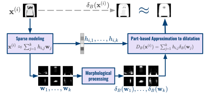
Figure 1: Process for computing the part-based-approximation of dilation.

2.2 Deep auto-encoders approaches

The main drawback of the NMF algorithm is that it is an offline process, the encoding of any new sample with regards to the previously learned basis $\mathbf{W}$ requires either to solve a computationally extensive constrained optimization problem, or to release the Non-Negativity constraint by using the pseudo-inverse $\mathbf{W^{+}}$ of the basis. The various approaches proposed to overcome this shortcoming rely on Deep Learning, and especially on deep auto-encoders, which are widely used in the representation learning field, and offer an online representation process.

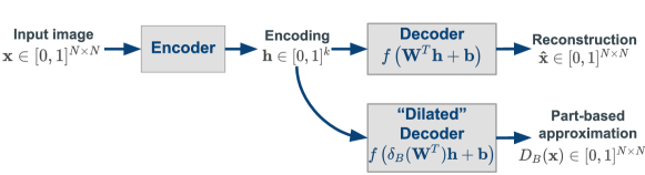
Figure 2: The auto-encoding process and the definition of part-based approximation to dilation by a structuring element $B$ in this framework.

An auto-encoder, as represented in Figure 2, is a model composed of two stacked neural networks, an encoder and a decoder whose parameters are trained by minimizing a loss function. A common example of loss function is the mean square error (MSE) between the input images $\mathbf{x}^{(i)}$ and their reconstructions by the decoder $\mathbf{\hat{x}}^{(i)}$:

$$L_{AE}=\frac{1}{M}\sum_{i=1}^{M}L(\mathbf{x}^{(i)},\mathbf{\hat{x}}^{(i)})=\frac{1}{M}\sum_{i=1}^{M}\frac{1}{N}||\mathbf{\hat{x}}^{(i)}-\mathbf{x}^{(i)}||_{2}^{2}.$$ (6)

In this framework, and when the decoder is composed of a single linear layer (possibly followed by a non-linear activation), the model approximates the input images as:

$$\mathbf{\hat{x}}^{(i)} =f\left(\mathbf{b}+\mathbf{h}^{(i)}\mathbf{W}\right) =f\left(\mathbf{b}+\sum_{j=1}^{k}h_{i,j}\mathbf{w}_{j}\right)$$ (7)

where $\mathbf{h}^{(i)}$ is the encoding of the input image by the encoder network, $\mathbf{b}$ and $\mathbf{W}$ respectively the bias and weights of the linear layer of the decoder, and $f$ the (possibly non-linear) activation function, that is applied pixel-wise to the output of the linear layer. The output $\mathbf{\hat{x}}^{(i)}$ is called the reconstruction of the input image $\mathbf{x}^{(i)}$ by the auto-encoder. It can be considered as a linear combination of atom images, up to the addition of an offset image $\mathbf{b}$ and to the application of the activation function $f$. The images of our learned dictionary are hence the columns of the weight matrix $\mathbf{W}$ of the decoder. We can extend the definition of part-based approximation, described in Section 2.1, to our deep-learning architectures, by applying the morphological operator to these atoms $\mathbf{w}_{1}$, …, $\mathbf{w}_{k}$, as pictured by the “dilated decoder” in Figure 2. Note that a central question lies in how to set the size $k$ of the latent space. This question is beyond the scope of this study and the value of $k$ will be arbitrarily fixed (we take $k=100$) in the following.

The NNSAE architecture, from Lemme et al. [11], proposes a very simple and shallow architecture for online part-based representation using linear encoder and decoder with tied weights (the weight matrix of the decoder is the transpose of the weight matrix of the encoder). Both the NCAE architectures, from Hosseini-Asl et al. [6] and the work from Ayinde et al. [2] that aims at extending it, drop this transpose relationship between the weights of the encoder and of the decoder, increasing the capacity of the model. Those three networks enforce the non-negativity of the elements of the representation, as well as the sparsity of the image encodings using various techniques.

2.2.1 Enforcing sparsity of the encoding

The most prevalent idea to enforce sparsity of the encoding in a neural network can be traced back to the work of H. Lee et al. [10]. This variant penalizes, through the loss function, a deviation $S$ of the expected activation of each hidden unit (i.e. the output units of the encoder) from a low fixed level $p$. Intuitively, this should ensure that each of the units of the encoding is activated only for a limited number of images. The resulting loss function of the sparse auto-encoder is then:

$$L_{AE}=\frac{1}{M}\sum_{i=1}^{M}L(\mathbf{x}^{(i)},\mathbf{\hat{x}}^{(i)})+\beta\sum_{j=1}^{k}S(p,\sum_{i=1}^{M}h_{j}^{(i)}),$$ (8)

where the parameter $p$ sets the expected activation objective of each of the hidden neurons, and the parameter $\beta$ controls the strength of the regularization. The function $S$ can be of various forms, which were empirically surveyed in [22]. The approach adopted by the NCAE [6] and its extension [2] rely on a penalty function based on the KL-divergence between two Bernoulli distributions, whose parameters are the expected activation and $p$ respectively, as used in [6]:

$$S(p,t_{j})=KL(p,t_{j})=p\log\frac{p}{t_{j}}+(1-p)\log\frac{1-p}{1-t_{j}}\;\;\mbox{ with }t_{j}=\sum_{i=1}^{M}h_{j}^{(i)}$$ (9)

The NNSAE architecture [11] introduces a slightly different way of enforcing the sparsity of the encoding, based on a parametric logistic activation function at the output of the encoder, whose parameters are trained along with the other parameters of the network.

2.2.2 Enforcing non-negativity of the decoder weights

For the NMF (Section 2.1) and for the decoder, non-negativity results in a part-based representation of the input images. In the case of neural networks, enforcing the non-negativity of the weights of a layer eliminates cancellations of input signals. In all the aforementioned works, the encoding is non-negative since the activation function at the output of the encoder is a sigmoid. In the literature, various approaches have been designed to enforce weight positivity. A popular approach is to use an asymmetric weight decay, added to the loss function of the network, to enact more decay on the negative weights that on the positive ones. However this approach, used in both the NNSAE [11] and NCAE [6] architectures, does not ensure that all weights will be non-negative. This issue motivated the variant of the NCAE architecture [2, 11], which uses either the $L_{1}$ rather than the $L_{2}$ norm, or a smoothed version of the decay using both the $L_{1}$ and the $L_{2}$ norms. The source code of that method being unavailable, we did not use this more recent version as a baseline for our study.

3 Proposed model

We propose an online part-based representation learning model, using an asymmetric auto-encoder with sparsity and non-negativity constraints.As pictured in Figure 3, our architecture is composed of two networks: a deep encoder and a shallow decoder (hence the asymmetry and the name of AsymAE we chose for our architecture). The encoder network is based on the discriminator of the infoGAN architecture introduced in [4], which was chosen for its average depth, its use of widely adopted deep learning components such as batch-normalization [8], 2D-convolutional layers [5] and leaky-RELU activation function [12]. It has been designed specifically to perform interpretable representation learning on datasets such as MNIST and Fashion-MNIST. The network can be adapted to fit to larger images. The decoder network is similar to the one presented in Figure 2. A Leaky-ReLU activation has been chosen after the linear layer. Its behavior is the same as the identity for positive entries, while it multiplies the negative ones by a fixed coefficient $\alpha_{lReLU}=0.1$. This activation function has shown better performances in similar architectures [12]. The sparsity of the encoding is achieved using the same approach as in [2, 6] that consists in adding to the previous loss function the regularization term described in Equations (8) and (9).

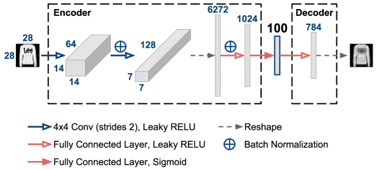
Figure 3: Our proposed auto-encoder architecture.

We only enforced the non-negativity of the weights of the decoder, as they define the dictionary of images of our learned representation and as enforcing the non-negativity of the encoder weights would bring nothing but more constraints to the network and lower its capacity. We enforced this non-negativity constraint explicitly by projecting our weights on the nearest points of the positive orthant after each update of the optimization algorithm (such as the stochastic gradient descent). The main asset of this other method that does not use any additional penalty functions, and which is quite similar to the way the NMF enforces non-negativity, is that it ensures positivity of all weights without the cumbersome search for good values of the parameters the various regularization terms in the loss function.

4 Experiments

To demonstrate the goodness and drawbacks of our method, we have conducted experiments on two well-known datasets MNIST [9] and Fashion MNIST [21]. These two datasets share common features, such as the size of the images ($28\times 28$), the number of classes represented ($10$), and the total number of images ($70000$), divided in a training set of $60000$ images and a test set of $10000$ images. We compared our method to three baselines: the sparse-NMF [7], the NNSAE [11], the NCAE [6]. The three deep-learning models (AsymAE (ours), NNSAE and NCAE) were trained until convergence on the training set, and evaluated on the test set. The sparse-NMF algorithm was ran and evaluated on the test set. Note that all models but the NCAE may produce reconstructions that do not fully belong to the interval $[0,1]$. In order to compare the reconstructions and the part-based approximation produced by the various algorithms, their outputs will be clipped between 0 and 1. There is no need to apply this operation to the output of NCAE as a sigmoid activation enforces the output of its decoder to belong to $[0,1]$. We used three measures to conduct this comparison:

• the reconstruction error, that is the pixel-wise mean squared error between the input images $\mathbf{x}^{(i)}$ of the test dataset and their reconstruction/approximation $\mathbf{\hat{x}}^{(i)}$: $\frac{1}{MN}\sum_{i=1}^{M}\sum_{j=1}^{N}(\mathbf{x}_{j}^{(i)}-\mathbf{\hat{x}}_{j}^{(i)})^{2}$;

• the sparsity of the encoding, measured using the mean on all test images of the sparsity measure $\sigma$ (Equation 2): $\frac{1}{M}\sum_{i=1}^{M}\sigma(\mathbf{h}^{(i)})$;

• the approximation error to dilation by a disk of radius 1, obtained by computing the pixel-wise mean squared error between the dilation $\delta_{B}$ by a disk of radius 1 of the original image and the part-based approximation $D_{B}$ to the same dilation, using the learned representation: $\frac{1}{MN}\sum_{i=1}^{M}\sum_{j=1}^{N}(D_{B}(\mathbf{x}^{(i)})_{j}-\delta_{B}(\mathbf{x}^{(i)})_{j})^{2}$.

The parameter settings used for NCAE and the NNSAE algorithms are the ones provided in [6, 11]. For the sparse-NMF, a sparsity constraint of $S_{h}=0.6$ was applied to the encodings and no sparsity constraint was applied on the atoms of the representation. For our AsymAE algorithm, $p=0.05$ was fixed for the sparsity objective of the regularizer of Equation (9), and the weight of the sparsity regularizer in the loss function in Equation (8) was set to $\beta=0.001$ for MNIST and $\beta=0.0005$ for Fashion-MNIST. Various other values have been tested for each algorithm, but the improvement of one of the evaluation measures usually came at the expense of the two others. Quantitative results are summarized in Table 1. Reconstructions by the various approaches of some sample images from both datasets are shown in Figure 4.

Table 1: Comparison of the reconstruction error, sparsity of encoding and part-based approximation error to dilation produced by the sparse-NMF, the NNSAE, the NCAE and the AsymAE, for both MNIST and Fashion-MNIST datasets.

Model Reconstruction Sparsity Part-based approximation error of code error to dilation MNIST Sparse-NMF $0.011$ $\mathbf{0.66}$ $\mathbf{0.012}$ NNSAE $0.015$ $0.31$ $0.028$ NCAE $0.010$ $0.35$ $0.18$ AsymAE $\mathbf{0.007}$ $0.54$ $0.069$ Fashion MNIST Sparse-NMF $0.011$ $\mathbf{0.65}$ $\mathbf{0.022}$ NNSAE $0.029$ $0.22$ $0.058$ NCAE $0.017$ $0.60$ $0.030$ AsymAE $\mathbf{0.010}$ $0.52$ $0.066$

Both the quantitative results and the reconstruction images attest the capacity of our model to reach a better trade-off between the accuracy of the reconstruction and the sparsity of the encoding (that usually comes at the expense of the former criteria), than the other neural architectures. Indeed, in all conducted experiments, varying the parameters of the NCAE and the NNSAE as an attempt to increase the sparsity of the encoding came with a dramatic increase of the reconstruction error of the model. We failed however to reach a trade-off as good as the sparse-NMF algorithm that manages to match a high sparsity of the encoding with a low reconstruction error, especially on the Fashion-MNIST dataset. The major difference between the algorithms can be seen in Figure 5 that pictures 16 of the 100 atoms of each of the four learned representations. While sparse-NMF manages, for both datasets, to build highly interpretable and clean part-based representations, the two deep baselines build representations that picture either too local shapes, in the case of the NNSAE, or too global ones, in the case of the NCAE. Our method suffers from quite the same issues as the NCAE, as almost full shapes are recognizable in the atoms. We noticed through experiments that increasing the sparsity of the encoding leads to less and less local features in the atoms. It has to be noted that the $L_{2}$ Asymmetric Weight Decay regularization used by the NCAE and NNSAE models allows for a certain proportion of negative weights. As an example, up to $32.2\%$ of the pixels of the atoms of the NCAE model trained on the Fashion-MNIST dataset are non-negative, although their amplitude is lower than the average amplitude of the positive weights. The amount of negative weights can be reduced by increasing the corresponding regularization, which comes at the price of an increased reconstruction error and less sparse encodings. Finally Figure 6 pictures the part-based approximation to dilation by a structuring element of size one, computed using the four different approaches on ten images from the test set. Although the quantitative results state otherwise, we can note that our approach yields a quite interesting part-based approximation, thanks to a good balance between a low overlapping of atoms (and dilated atoms) and a good reconstruction capability.

(a)

(b)

(c)

(d)

(e)

Figure 4: Reconstruction of the Fashion-MNIST dataset (first row) by the sparse-NMF, the NNSAE, the NCAE and the AsymAE.

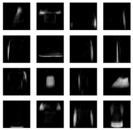
(a) Sparse-NMF

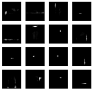
(b) NNSAE

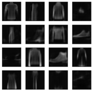
(c) NCAE

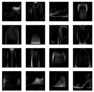
(d) AsymAE

Figure 5: 16 of the 100 atom images of the four compared representations of Fashion-MNIST dataset.

(a)

(b)

(c)

(d)

(e)

Figure 6: Part-based approximation of the dilation by a structuring element of size 1 (first row), computed using the sparse-NMF, the NNSAE, the NCAE and the AsymAE.

5 Conclusions and future works

We have presented an online method to learn a part-based dictionary representation of an image dataset, designed for accurate and efficient approximations of morphological operators. This method relies on auto-encoder networks, with a deep encoder for a higher reconstruction capability and a shallow linear decoder for a better interpretation of the representation. Among the online part-based methods using auto-encoders, it achieves the state-of-the-art trade-off between the accuracy of reconstructions and the sparsity of image encodings. Moreover, it ensures a strict (that is, non approximated) non-negativity of the learned representation. These results would need to be confirmed on larger and more complex images (e.g. color images), as the proposed model is scalable. We especially evaluated the learned representation on an additional criterion, that is the commutation of the representation with a morphological dilation, and noted that all online methods perform worse than the offline sparse-NMF algorithm. A possible improvement would be to impose a major sparsity to the dictionary images an appropriate regularization. Additionally, using a morphological layer [3, 16] as a decoder may be more consistent with our definition of part-based approximation, since a representation in the $(\max,+)$ algebra would commute with the morphological dilation by essence.

Acknowledgments:

This work was partially funded by a grant from Institut Mines-Telecom and MINES ParisTech.

References

- [1] Angulo, J., Velasco-Forero, S.: Sparse mathematical morphology using non-negative matrix factorization. In: Soille, P., Pesaresi, M., , Ouzounis, G.K. (eds.) 10th International Symposium on Mathematical Morphology and Its Application to Signal and Image Processing (ISMM). vol. LNCS 6671, pp. 1–12 (2011)
- [2] Ayinde, B.O., Zurada, J.M.: Deep learning of constrained autoencoders for enhanced understanding of data. CoRR abs/1802.00003 (2018)
- [3] Charisopoulos, V., Maragos, P.: Morphological perceptrons: Geometry and training algorithms. pp. 3–15 (04 2017). https://doi.org/10.1007/978-3-319-57240-6_1
- [4] Chen, X., Duan, Y., Houthooft, R., Schulman, J., Sutskever, I., Abbeel, P.: Infogan: Interpretable representation learning by information maximizing generative adversarial nets. CoRR abs/1606.03657 (2016)
- [5] Dosovitskiy, A., Springenberg, J.T., Brox, T.: Learning to generate chairs with convolutional neural networks. CoRR abs/1411.5928 (2014)
- [6] Hosseini-Asl, E., Zurada, J.M., Nasraoui, O.: Deep learning of part-based representation of data using sparse autoencoders with nonnegativity constraints. IEEE Transactions on Neural Networks and Learning Systems 27(12), 2486–2498 (2016)
- [7] Hoyer, P.O.: Non-negative matrix factorization with sparseness constraints. CoRR cs.LG/0408058 (2004)
- [8] Ioffe, S., Szegedy, C.: Batch normalization: Accelerating deep network training by reducing internal covariate shift. CoRR abs/1502.03167 (2015)
- [9] LeCun, Y., Cortes, C.: MNIST handwritten digit database (2010), http://yann.lecun.com/exdb/mnist/
- [10] Lee, H., Ekanadham, C., Ng, A.Y.: Sparse deep belief net model for visual area v2. In: Platt, J.C., Koller, D., Singer, Y., Roweis, S.T. (eds.) Advances in Neural Information Processing Systems 20, pp. 873–880 (2008)
- [11] Lemme, A., Reinhart, R.F., Steil, J.J.: Online learning and generalization of parts-based image representations by non-negative sparse autoencoders. Neural Networks 33, 194–203 (2012)
- [12] Maas, A.L.: Rectifier nonlinearities improve neural network acoustic models. In: International Conference on Machine Learning (2013)
- [13] Mairal, J., Bach, F.R., Ponce, J.: Sparse modeling for image and vision processing. CoRR abs/1411.3230 (2014)
- [14] Maragos, P., Schafer, R.: Morphological skeleton representation and coding of binary images. IEEE Transactions on Acoustics, Speech, and Signal Processing 34(5), 1228–1244 (1986)
- [15] Pesaresi, M., Benediktsson, J.A.: A new approach for the morphological segmentation of high-resolution satellite imagery. IEEE Transactions on Geoscience and Remote Sensing 39(2), 309–320 (2001)
- [16] Ritter, G., Sussner, P.: An introduction to morphological neural networks. vol. 4, pp. 709 – 717 vol.4 (09 1996). https://doi.org/10.1109/ICPR.1996.547657
- [17] Soille, P.: Morphological image analysis: principles and applications. Springer Science & Business Media (2013)
- [18] Tanaka, K.: Columns for complex visual object features in the inferotemporal cortex: clustering of cells with similar but slightly different stimulus selectivities. Cerebral Cortex 13 1, 90–9 (2003)
- [19] Theis, F.J., Stadlthanner, K., Tanaka, T.: First results on uniqueness of sparse non-negative matrix factorization. In: 13th IEEE European Signal Processing Conference. pp. 1–4 (2005)
- [20] Velasco-Forero, S., Angulo, J.: Non-Negative Sparse Mathematical Morphology, vol. 202, chap. 1. Elsevier Inc.Academic Press (2017)
- [21] Xiao, H., Rasul, K., Vollgraf, R.: Fashion-MNIST: a novel image dataset for benchmarking machine learning algorithms. arXiv:1708.07747 (2017)
- [22] Zhang, L., Lu, Y.: Comparison of auto-encoders with different sparsity regularizers. In: International Joint Conference on Neural Networks (IJCNN). pp. 1–5 (2015)