Non-rigid 3D shape retrieval based on multi-view metric learning

Abstract

This study presents a novel multi-view metric learning algorithm, which aims to improve 3D non-rigid shape retrieval. With the development of non-rigid 3D shape analysis, there exist many shape descriptors. The intrinsic descriptors can be explored to construct various intrinsic representations for non-rigid 3D shape retrieval task. The different intrinsic representations (features) focus on different geometric properties to describe the same 3D shape, which makes the representations are related. Therefore, it is possible and necessary to learn multiple metrics for different representations jointly. We propose an effective multi-view metric learning algorithm by extending the Marginal Fisher Analysis (MFA) into the multi-view domain, and exploring Hilbert-Schmidt Independence Criteria (HSCI) as a diversity term to jointly learning the new metrics. The different classes can be separated by MFA in our method. Meanwhile, HSCI is exploited to make the multiple representations to be consensus. The learned metrics can reduce the redundancy between the multiple representations, and improve the accuracy of the retrieval results. Experiments are performed on SHREC’10 benchmarks, and the results show that the proposed method outperforms the state-of-the-art non-rigid 3D shape retrieval methods.

Index Terms—  Non-rigid shape retrieval, Multi-view learning, Metric learning, Marginal Fisher Analysis

1 Introduction

With the rapid development of 3D model acquirement technique, massive amounts of 3D shape data had been captured and many large-scale 3D shape datasets were created, such as Google 3D warehouse, Shapenet, etc. The 3D shape analysis has been an active research spot for decades. Among numerous challenges in 3D shape analysis, non-rigid 3D shape retrieval [1] is one of the most important problems. The 3D shape retrieval can be simply described as follows: Given a query shape, we would like to develop a algorithm to determinate the similarity of the query shape to all the shapes in a large collection of 3D shapes. Most conventional non-rigid 3D shape retrieval approaches compute the similarity between the shapes based on a hand-crafted representation and metric. Once the representations of the shapes are obtained, one can explore a metric to measure the similarity of the representations for retrieval task. However, only one type representation usually can not contain enough geometric structure information to characterize the shapes with non-rigid deformations well. Therefore, making full use of the geometric properties by multiple representations [2] to improve the shape retrieval [3] is a hot topic.

In the past years, various approaches for non-rigid 3D shape retrieval has been proposed [4, 5, 6, 7]. Most of these approaches mainly focus on construction of the intrinsic representation and calculation of similarity between the representations [8]. The intrinsic representations are usually constructed based on the intrinsic descriptors by using various approaches such as BoW (Bag of Words) and locality constrained linear coding (LLC). The past decade a large number of shape intrinsic descriptors have been extracted based on Laplace-Beltrami operator for non-rigid 3D shape analysis, such as ShapeDNA [9], Heat Kernel Signature ($HKS$) [10], scale-invariant Heat Kernel Signature ($siHKS$) [11] and Wave Kernel Signature ($WKS$) [12], etc. A comprehensive survey in [13] has provided details of these spectral signatures. In [4], the authors utilized bag-of-words (BoW) to construct the representation. A set of spectral signatures such as $HKS$, $WKS$, etc., were clustered by k-means to construct the dictionary of words. Then they added the spatial information into the histogram as shape representation. At last, Similarity Sensitive Hashing (SSH) was explored to improve the performance of the retrieval. Unlike the standard BoW methods, the authors of [5] proposed a supervised learning of BoW approach with weighted mean pooling to form the representation. In [6], it explored auto-encoder to optimize the histogram of $HKS$. These methods pay more attention to the construction of the representation, and the similarity between the rpresentation usually based on Euclidean metric. Some methods utilized metric learning method to get a new metric for improving their performance. The authors of [14] obtained the representation by utilizing a weighted mean pooling on point signatures, and linearly mapped into subspace by Large Margin Nearest Neighbor (LMNN) algorithm directly. These methods usually utilize one intrinsic descriptor to form the representation, which can not contain enough geometric information for 3D shape retrieval on large-scale 3D shape datasets. Multiple descriptors should be utilized to tackle this problem. Although descriptors from different views reflect different properties of one same shape, they contain compatible and complementary geometric information which can improve the retrieval performance. And the methods that explored multiple descriptors to construct the hiotellis2016Nonshape representation. For example, in [15], the authors compute the weighted average of the distance between the representations constructed by single descriptor. However, these concatenating multiple features methods is not physically meaningful, and caused over-fitting on a small training sample [16]. Thus we develop an multi-view metric learning method combining multiple types representation to achieve the improvement of performance compared to single-view methods for non-rigid 3D shape retrieval.

Generally speaking, metric learning methods [17] usually aim to learn a metric function so that the distance between the data under new metric can be consistent with their labels. In past years, a large number of metric learning methods have been proposed [18, 19, 20, 21, 22] such as PCA , LMNN , SVMs , ITML , LDA , LPP etc., which are widely utilized in real-word applications. Meanwhile, a great many methods of learning from multi-view data have also been proposed [23]. Single-view methods always drop some information of the data, which affects the performance. Multi-view learning methods [24] can tackle this problem by considering different views jointly, which can fully exploit information from multiple views to improve the performance. Multi-view learning methods mainly exploit consensus principle or complementary principle to improve learning performance. You can read a survey about multi-view learning methods in [16]. In this paper, we propose a novel multi-view metric learning method for non-rigid 3D shape retrieval, which can fully utilize the geometric information by jointly learning multiple metrics. To this end, we develop a multi-view metric algorithm named Marginal Fisher Analysis Multi-view Metric learning (MFAMML). We utilize MFA to seek for the optimal projections, which considers both local manifold structure and label information. Since projections can maintain the local manifold structure and maximize the class separability simultaneously, it can potentially achieve higher performance than Euclidean distance metrics in original feature space. Furthermore, the Hilbert-Schmidt Independence Criterion (HSIC) is employed measure the dependence among different views, which can co-regularize different views and enforce them to be consistent in kernel space. With HSIC term, we can explore the compatible and complementarity information from different views. At last, the alternating maximization is carried out for optimizing the proposed approach. Figure1. shows the pipeline of the proposed framework.

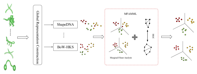
Fig. 1: pipeline of Our proposed framework.

2 Background

In this section, we briefly review the concept of Mahalanaobis distance. Similar to most of the metric learning methods, which aims to seek Mahalanobis distance for specific application, we also focus on find the Mahalanobis distance functions. Generally, given a sample set $X=[x_{1},x_{2},...,x_{1=N}]\in R^{d\times N}$ with $N$ samples and $x_{k}\in R^{d\times 1}$, the definition of the Mahalanobis distance between $x_{i}$ and $x_{j}$ is as:

$$d_{M}(x_{i},x_{j})=\sqrt{(x_{i}-x{j})^{T}M(x_{i}-x_{j})}$$

The $d_{M}(x_{i},x_{j})$ should be satisfied the properties of nonnegativity, symmetry, identity of indiscernible, and triangle inequality, which are from definition of distance function. Hence, $M$ must be a symmetric PSD matrix, and can be decomposed by as:

$$M=WW^{T}$$

where $W\in R^{d\times p}$. Therefore, learning a Mahalanobis distance metric $M$ is equivalent to seeking a linear projection $W$, which projects the sample $x_{i}$ to a new space. The learned Mahalanobis metric is equal to the Euclidean metric in the new space.

3 Proposed Approach

In this section, we present the detail of the MFAMML method for non-rigid 3D shape retrieval. We extract different types of 3D shape descriptors to construct representations. Some global descriptors that contain the global geometric structure information can be used as the representation directly, such as ShapeDNA, Modal Function Transformation (MFT), etc. For some point signatures such as $HKS$, $siHKS$, $WKS$, etc. should be encoded by BoW method to form the representations of the shapes. Once the multiple representations are constructed, we use these representations as inputs to learning the metrics for every representation jointly. For single view, the new metric maximize the between-class separability. Meanwhile, every representation is enforced to be consistent by HSIC term, which makes the multiple representations to be more discriminative under the new metric by integrating the compatible and complementarity information from different representation. At last, every representation is projected in a new space and concatenated for shape retrieval.

3.1 The Process of MFAMML

We first introduce the MFA algorithm [25] for a single view representation $X^{v}$. Let $X^{v}=[x^{v}_{1},x^{v}_{2},...,x^{v}_{N}],\ x^{v}_{i}\in R^{n_{v}},\ v=1,2,...,m$, denote the $v-$th view of $N$ samples, and the dimension of it is $n_{v}$. Let $G_{v}=\{X_{v},S_{v}\}$ be the similarity graph with the vertex set $X^{v}$ and similarity matrix $S_{v}$. And the corresponding degree matrix $D_{v}$ and laplace matrix $L_{v}$ are as follows:

$$L_{v}=D_{v}-S_{v},D^{ii}_{v}=\sum_{j\neq i}S^{ij}_{v}\quad\forall i.$$

The graph embedding algorithm is to compute a low-dimensional representation of the vertex set, which can preserves the similarities between pairs of data point in orginal space. Standard graph embedding algorithm aims to find the low-dimensional embedding of vertices as $Y^{v}=[y^{v}_{1},y^{v}_{2},...,y^{v}_{N}]$, which can maintain the similarities among the vertex pairs:

$$\begin{split}Y^{v}_{*}=\underset{Y^{v}}{argmin}Tr(Y^{v}L_{v}(Y^{v})^{T})\\ \text{with}\quad Tr(Y^{v}B_{v}(Y^{v})^{T})=c.\end{split}$$ (1)

where $c_{v}$ is a constant and $Tr(A)$ is the trace of matrix $A$. Matrix $B_{v}$ is the constraint matrix based on some more general constraints among the vertices.

The MFA fit the linearization formulation of the graph embedding framework. It considers the label information into the graph embedding, and aims to obtain a projection with considering both local manifold structure and label information. The objective function of it is defined as:

$$\begin{split}W^{v}_{*}=\underset{W^{v}}{argmax}Tr((W^{v})^{T}X^{v}B_{v}(X^{v})^{T}W^{v}.\\ \text{with}\quad Tr((W^{v})^{T}X^{v}L_{v}(X^{v})^{T}W^{v})=c_{v}\end{split}$$ (2)

where the $W^{v}\in R^{n_{v}}\times d$ is the projection matrix. In this version, the $B$ and $L$ are defined as:

$$S_{v}^{ij}=\begin{cases}1,&\text{if}\ i\in N_{k_{1}}(j)\ \text{or}\ j\in N_{k_{1}}(i)\\ 0,&\text{else}\end{cases}$$

$$\overline{S_{v}^{ij}}=\begin{cases}1,&\text{if}\ (i,j)\in P_{k_{2}}(l(x^{v}_{j}))\ \text{or}\ (i,j)\in P_{k_{2}}(l(x^{v}_{i}))\\ 0,&\text{else}\end{cases}$$

$$L_{v}=D_{v}-S_{v}\ D^{ii}_{v}=\sum_{j\neq i}S^{ij}_{v}\quad\forall i$$

$$B_{v}=\overline{D_{v}}-\overline{S_{v}}\ \overline{D^{ii}_{v}}=\sum_{j\neq i}\overline{S^{ij}_{v}}\quad\forall i$$

where the $N_{k_{1}}(i)$ is the index set of which $k_{1}$ nearest neighbors of $x^{v}_{i}$ have the same label with $x^{v}_{i}$.

From the construction of the graph of MFA, we can see that MFA can explore both label information and local manifold structure. Therefore, the learned new metric (projection) can ensure the within-class compactness and class separability simultaneously. Inspired the MFA, we can get a multi-view version of MFA algorithm with the optimization objective function:

$$\begin{split}J=\underset{W^{v}}{max}\ \sum_{v=1}^{m}{Tr((W^{v})^{T}X^{v}B_{v}(X^{v})^{T}W^{v}})\\ \text{with}\quad Tr((W^{v})^{T}X^{v}L_{v}(X^{v})^{T}W^{v})=c_{v}\quad\forall v=1...m\end{split}$$ (3)

Although multiple types of representations of the shapes are extracted by different approaches, they are highly related since they are descriptions of the same shape. In order to guarantee the consensus principle, we make the hypotheses that the pairwise similarities of the representations are similar across all types of them. The hypotheses means that similarity matrixes of multiple types of representations should be consistent under the new metrics. Therefore, we employ the Hilbert-Schmidt Independence Criterion (HSIC) [26] as a measurement of dependence between the multiple types of shape representations. In the MFAMML, the HSIC for any two types of representation can be simplified as:

$$\begin{split}&HSIC(X^{v},X^{t})=(N-1)^{-2}Tr(K_{v}HK_{t}H)\\ &=(n-1)^{-2}Tr((W^{v})^{T}X^{v}HK_{t}H(X^{v})^{T}W^{v})\end{split}$$ (4)

where the inner product kernel function is as:

$$K_{v}=(X^{v})^{T}W^{v}(W^{v})^{T}X^{v}.$$

In order to ensure our hypotheses, we use HSIC about any two types of representations to penalize for independence between them, which can make them to be consistent. Combine this with the MFA objectives for individual views Eq.4, we can get the following the objective function:

$$\begin{split}J=\underset{W^{v}}{max}\ \sum_{v=1}^{m}{Tr((W^{v})^{T}X^{v}B_{v}(X^{v})^{T}W^{v}})\\ +\lambda\sum_{w\neq i}^{m}Tr((W^{v})^{T}X^{v}HK_{w}H(X^{v})^{T}W^{v})\\ s.t.\quad Tr((W^{v})^{T}X^{v}L_{v}(X^{v})^{T}W^{v})=c_{v}\quad\forall v=1...m\end{split}$$ (5)

where the $\lambda>0$ is a a trade-off parameter between two terms of Eq[ref]. The first term ensure the class separability within each view for the most discrimination while the second one follows the hypotheses. We can find that seeking each projection $W^{v}$ exploits all other $W^{t},\ t\neq v$. Therefore, maximizing Eq5 aims to find the new projections for every view, which can integrate the geometric information from multiple types of representation.

3.2 The Optimization Procedure Of MAFMML

In this section, we introduce the details of optimizing the MFAMML. In order to find the optimal solution of objective function, we rewrite the objective function firstly:

$$\begin{split}J&=\ \underset{W^{v}}{max}\ \sum_{v=1}^{m}{Tr((W^{v})^{T}X^{v}B_{v}(X^{v})^{T}W^{v}})\\ &+\lambda\sum_{w\neq i}^{m}Tr((W^{v})^{T}X^{v}HK_{w}H(X^{v})^{T}W^{v})\\ &=\underset{W^{v}}{max}\ \sum_{v=1}^{m}{Tr((W^{v})^{T}P_{v}W^{v})}\\ &s.t.\quad Tr((W^{v})^{T}X^{v}L_{v}(X^{v})^{T}W^{v})=c_{v}\quad\forall v=1...m\end{split}$$ (6)

where

$$\begin{split}&P_{v}=F+\lambda G_{v},\quad F=X^{v}B_{v}(X^{v})^{T},\quad\\ &G_{v}=\sum_{w=1;w\neq v}^{m}X^{v}HK_{w}H(X^{v})^{T}.\end{split}$$ (7)

The maximization problem is transforms into an iterative alternating optimization problem. First, we initialize all $W^{v},\ v=1,...,m$ by the solution of MFA for single view. We solve the objective of Eq7 by optimizing each of single $W^{t}$ at one time, keeping all other variables fixed. The optimization problem for $W^{v}$ is as:

$$\begin{split}&\underset{W^{v}}{max}\ Tr((W^{v})^{T}P_{v}W^{v})\\ &s.t.\quad Tr((W^{v})^{T}X^{v}L_{v}(X^{v})^{T}W^{v})=c_{v}.\\ \end{split}$$ (8)

Obviously, optimization Eq.LABEL:Eq:11 can be converted into the following equation:

$$\begin{split}&\underset{W^{v}}{max}\ \frac{Tr((W^{v})^{T}P_{v}W^{v})}{Tr((W^{v})^{T}X^{v}L_{v}(X^{v})^{T}W^{v})}\end{split}$$ (9)

Eq.9 is a standard Trace Ratio problem. Therefore, all the projection matrixes can be updated using Eq.9 respectively, which can be solved easily by Generalized Eigenvalue Decomposition (GED) algorithm. The iterative alternating optimization of MFAMML stops when all projection matrixes $W^{v}$ converges. Once $W^{v}$s are learned, we can obtain the new metrics $M_{v}=W^{v}(W^{v})^{T}$ for all types of the representations. Then we can compute the distance between every pair of the shapes as:

$$d(i,j)=\sum^{m}_{v=1}(x^{v}_{i}-x^{v}_{j})^{T}M_{v}(x^{v}_{i}-x^{v}_{j}).$$ (10)

4 Experiments

We conduct experiments on SHREC’10 datasets and compare out method with state-of-the-art methods. The standard of evaluation is based on these quantitative measure from PSB [27]: Nearest Neighbor (NN), First Tier (FT), Second Tier (ST), Emeasure (E), and Discounted Cumulative Gain (DCG).

4.1 Parameters Setting

For these two 3D shape datasets, we extract ShapeDNA, $HKS$, $WKS$, $siHKS$ spectral descriptors to form multiple types of shape representation. The ShapeDNA is used as the representation directly, other point descriptors are coded by BoW to form global representations. These spectral descriptors is shown as follows:

• (1) ShapeDNA [9]: The ShapeDNA is obtained by truncating the sequence of the eigenvalues of the LBO. Then it is normalized by the first eigenvalue. ShapeDNA is a global descriptor which has various properties such as the simple representation, comparison, scale invariance, ect. And in spite of its simplicity, it has a good performance for non-rigid shape retrieval.

• (2) $HKS$ [10]: The $HKS$ is a point descriptor, which is defined as the diagonal element of the heat kernel based on the concept of heat diffusion over a surface, which represent that the amount of heat remaining at the point over a period of time. It has many advantages properties, such as intrinsic, multi-scale, informative and robust property.

• $siHKS$ [11]: The $siHKS$ is a point descriptor, which is constructed based on $HKS$. The Fourier transform is utilized for moving scale factor from the time domain to the frequency domain. Therefore, $siHKS$ is invariant for the change of the shape scale.

• $WKS$ [12]: The physical significance of $WKS$ is the average probability of a quantum mechanical particle at a specific location. The $WKS$ clearly separates influences of different frequencies, treating all frequencies equally. Therefore, the $WKS$ can take more geometric details than $HKS$.

The first 35 normalized eigenvalues of the LBO are utilized as the ShapeDNA. Next, we explore first 100 eigenvectors and eigenvalues of LBO to compute the $HKS$, $siHKS$ and $WKS$ of every point for all the shapes. 50-dimensional $HKS$, $siHKS$ and 100-dimensional $WKS$ are obtained with same parameters setting in [ChiotellisTWC16]. Then, we utilize the BoW algorithm to construct the three types of representations based on three point signatures, and these representations are all 64-dimensional.

4.2 Experiment On SHREC’10

SHREC’10 batabase [28] consists of 200 watertight 3D triangular meshes. The dataset is classified into 10 categories based on their semantic (isometric), and each class contains 20 objects with distinct postures. To evaluate the performance of our algorithm, 2 experiments on SHREC’10 dataset are conducted. We compare our approach with the methods related with LBO: (1) ShapeGoogle, (2) Modal Function Transformation (MFT), (3)Supervised Dictionary Learning (SupDL), and these four representations without our algorithm. 50% samples are randomly selected to train MFAMML and left 50% samples are as testing set. The PR(precision-recall)-curves are shown in Fig.2. For next experiment, we compare our approach with these methods: MR-BF-DSIFT-E, DMEVD and CF, which are summarized in [28]. In this experiment, we select 50% samples randomly to train MFAMML also, and utilize all the dataset as the testing set for comparing. Table 1 shows the comparison between our methods and the methods summarized in [28].

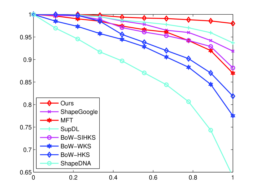
Fig. 2: Comparison of the precision Recall curves (PR-curves) among our method and the other methods on SHREC10 Non-rigid dataset.

Table 1: Five quantitative measures on SHREC’11

Method	NN	FT	ST	E	DCG
MR-BF-DSIFT-E	98.5	90.9	96.3	70.6.9	97.6
DMEVD	100.0	86.3	95.7	70.1	97.7
CF	92.0	63.5	78.0	55.3	87.8
Our method	100.0	99.5	99.7	73.5	99.8

4.3 Experiment Results

We can see that our performance out-performs the ShapeDNA, ShapeGoogle, SupDL, and the single representations from Fig.2 . We then compare the methods summarized in SHREC’10. We see that our results is comparable to the best performing on these two datasets from Table1. Our methods obtain the best performance among the state-of-the-art methods on the common two datasets. These results verify the performance of the MFAMML method.

5 Conclusion

In this paper, we proposed a novel multi-view metric learning method for non-rigid 3D shape retrieval. MAFMML aims to overcome that one type of representation can not contains enough geometric information for retrieval task. The MAFMML can explore compatible and complementary geometric information from multiple intrinsic representations. For each type of representation, MFAMML learns a new metric for every representation by maximizing the distance between extra-class pair data points with inner-class pair fixed. Meanwhile, the HSIC is used to ensure the consistence across different types of representation. Therefore, MAFMML can integrates compatible information from multiple types of representations. Our approach is simple to implement and easy to optimize. Results of experiments on SHREC’10 benchmark datasets have proved the advantages of our approach over state-of-the-art non-rigid 3D shape retrieval methods.

References

- [1] Lin Wu, Yang Wang, and Ling Shao, “Cycle-consistent deep generative hashing for cross-modal retrieval,” IEEE Transactions on Image Processing, vol. 28, no. 4, pp. 1602–1612, 2019.
- [2] Lin Wu, Yang Wang, Ling Shao, and Meng Wang, “3-d personvlad: Learning deep global representations for video-based person reidentification,” IEEE transactions on neural networks and learning systems, 2019.
- [3] Yang Wang, Xuemin Lin, Lin Wu, and Wenjie Zhang, “Effective multi-query expansions: Collaborative deep networks for robust landmark retrieval,” IEEE Transactions on Image Processing, vol. 26, no. 3, pp. 1393–1404, 2017.
- [4] Alexander M. Bronstein, Michael M. Bronstein, Leonidas J. Guibas, and Maks Ovsjanikov, “Shape google: Geometric words and expressions for invariant shape retrieval,” ACM Trans. Graph., vol. 30, no. 1, pp. 1:1–1:20, 2011.
- [5] Roee Litman, Alexander M. Bronstein, Michael M. Bronstein, and Umberto Castellani, “Supervised learning of bag-of-features shape descriptors using sparse coding,” Comput. Graph. Forum, vol. 33, no. 5, pp. 127–136, 2014.
- [6] Jin Xie, Yi Fang, Fan Zhu, and Edward Wong, “Deepshape: Deep learned shape descriptor for 3d shape matching and retrieval,” in Proceedings of the IEEE Conference on Computer Vision and Pattern Recognition, 2015, pp. 1275–1283.
- [7] Hamed Ghodrati and A. Ben Hamza, “Nonrigid 3d shape retrieval using deep auto-encoders,” Applied Intelligence, vol. 47, no. 1, pp. 1–18, 2017.
- [8] Lin Wu, Yang Wang, Xue Li, and Junbin Gao, “Deep attention-based spatially recursive networks for fine-grained visual recognition,” IEEE transactions on cybernetics, vol. 49, no. 5, pp. 1791–1802, 2019.
- [9] Martin Reuter, Franz-Erich Wolter, and Niklas Peinecke, “Laplace-beltrami spectra as ’shape-dna’ of surfaces and solids,” Computer-Aided Design, vol. 38, no. 4, pp. 342–366, 2006.
- [10] Jian Sun, Maks Ovsjanikov, and Leonidas J. Guibas, “A concise and provably informative multi-scale signature based on heat diffusion,” Comput. Graph. Forum, vol. 28, no. 5, pp. 1383–1392, 2009.
- [11] Michael M. Bronstein and Iasonas Kokkinos, “Scale-invariant heat kernel signatures for non-rigid shape recognition,” in The Twenty-Third IEEE Conference on Computer Vision and Pattern Recognition, CVPR 2010, San Francisco, CA, USA, 13-18 June 2010, 2010, pp. 1704–1711.
- [12] Mathieu Aubry, Ulrich Schlickewei, and Daniel Cremers, “The wave kernel signature: A quantum mechanical approach to shape analysis,” in IEEE International Conference on Computer Vision Workshops, ICCV 2011 Workshops, Barcelona, Spain, November 6-13, 2011, 2011, pp. 1626–1633.
- [13] Chunyuan Li and A. Ben Hamza, “Spatially aggregating spectral descriptors for nonrigid 3d shape retrieval: a comparative survey,” Multimedia Syst., vol. 20, no. 3, pp. 253–281, 2014.
- [14] Ioannis Chiotellis, Rudolph Triebel, Thomas Windheuser, and Daniel Cremers, Non-rigid 3D Shape Retrieval via Large Margin Nearest Neighbor Embedding, 2016.
- [15] Ryutarou Ohbuchi and Takahiko Furuya, “Distance metric learning and feature combination for shape-based 3d model retrieval,” in Proceedings of the ACM workshop on 3D object retrieval, 3DOR ’10, Firenze, Italy, October 25, 2010, 2010, pp. 63–68.
- [16] Xu Chang, Dacheng Tao, and Xu Chao, “A survey on multi-view learning,” Computer Science, 2013.
- [17] Lin Wu, Yang Wang, Junbin Gao, and Xue Li, “Where-and-when to look: Deep siamese attention networks for video-based person re-identification,” IEEE Transactions on Multimedia, 2018.
- [18] Yang Wang, Xuemin Lin, Lin Wu, Wenjie Zhang, Qing Zhang, and Xiaodi Huang, “Robust subspace clustering for multi-view data by exploiting correlation consensus,” IEEE Transactions on Image Processing, vol. 24, no. 11, pp. 3939–3949, 2015.
- [19] Lin Feng, Huibing Wang, Bo Jin, Haohao Li, Mingliang Xue, and Le Wang, “Learning a distance metric by balancing kl-divergence for imbalanced datasets,” IEEE Transactions on Systems, Man, and Cybernetics: Systems, , no. 99, pp. 1–12, 2018.
- [20] Huibing Wang, Lin Feng, Jing Zhang, and Yang Liu, “Semantic discriminative metric learning for image similarity measurement,” IEEE Transactions on Multimedia, vol. 18, no. 8, pp. 1579–1589, 2016.
- [21] Yang Wang, Wenjie Zhang, Lin Wu, Xuemin Lin, Meng Fang, and Shirui Pan, “Iterative views agreement: An iterative low-rank based structured optimization method to multi-view spectral clustering,” in International Joint Conference on Artificial Intelligence, 2016, pp. 2153–2159.
- [22] Yang Wang, Lin Wu, Xuemin Lin, and Junbin Gao, “Multiview spectral clustering via structured low-rank matrix factorization,” IEEE transactions on neural networks and learning systems, vol. 29, no. 10, pp. 4833–4843, 2018.
- [23] C. Christoudias, Raquel Urtasun, and Trevor Darrell, “Multi-view learning in the presence of view disagreement,” Uai, 2012.
- [24] Huibing Wang, Lin Feng, Laihang Yu, and Jing Zhang, “Multi-view sparsity preserving projection for dimension reduction,” Neurocomputing, vol. 216, pp. 286–295, 2016.
- [25] Xu Dong, Yan Shuicheng, Tao Dacheng, Lin Stephen, and Zhang Hong-Jiang, “Marginal fisher analysis and its variants for human gait recognition and content- based image retrieval,” IEEE Transactions on Image Processing, vol. 16, no. 11, pp. 2811–2821, 2007.
- [26] Arthur Gretton, Olivier Bousquet, Alex Smola, and Bernhard Schölkopf, Measuring Statistical Dependence with Hilbert-Schmidt Norms, 2005.
- [27] P. Shilane, P. Min, M. Kazhdan, and T. Funkhouser, “The princeton shape benchmark,” in Proceedings Shape Modeling Applications, 2004., June 2004, pp. 167–178.
- [28] Z. Lian, A. Godil, T. Fabry, T. Furuya, J. Hermans, R. Ohbuchi, C. Shu, D. Smeets, P. Suetens, D. Vandermeulen, and S. Wuhrer, “Shrec’10 track: Non-rigid 3d shape retrieval,” in Proceedings of the 3rd Eurographics Conference on 3D Object Retrieval, Aire-la-Ville, Switzerland, Switzerland, 2010, 3DOR ’10, pp. 101–108, Eurographics Association.