Affect in Tweets Using Experts Model

Abstract

Estimating the intensity of emotion has gained significance as modern textual inputs in potential applications like social media, e-retail markets, psychology, advertisements etc., carry a lot of emotions, feelings, expressions along with its meaning. However, the approaches of traditional sentiment analysis primarily focuses on classifying the sentiment in general (positive or negative) or at an aspect level(very positive, low negative, etc.) and cannot exploit the intensity information. Moreover, automatically identifying emotions like anger, fear, joy, sadness, disgust etc., from text introduces challenging scenarios where single tweet may contain multiple emotions with different intensities and some emotions may even co-occur in some of the tweets. In this paper, we propose an architecture, Experts Model, inspired from the standard Mixture of Experts (MoE) model. The key idea here is each expert learns different sets of features from the feature vector which helps in better emotion detection from the tweet. We compared the results of our Experts Model with both baseline results and top five performers of SemEval-2018 Task-1, Affect in Tweets (AIT). The experimental results show that our proposed approach deals with the emotion detection problem and stands at top-5 results.

1 Introduction

Sentiment analysis is one of the most famous Natural Language Processing (NLP) tasks. This task was used in social network services [Pang et al., 2008, Asur and Huberman, 2010], e-retailing, advertising [Qiu et al., 2010, Jin et al., 2007], question answering systems [Somasundaran et al., 2007, Stoyanov et al., 2005] and many other domains. It focuses on the automatic prediction of polarity or sentiment on tweets or reviews. While most computer science research in this field has focused on strict positive/negative sentiment analysis, the three dominant theories [Marsella et al., 2010, Stelmack and Stalikas, 1991] of emotion agree that humans express or operate with much more nuanced emotion representations. In other words, tweets or reviews, in recent times, include non-standard representations of emotion like emoticons, emojis etc. This task of sentiment analysis became increasingly complex due to an addition of creatively spelt words (for eg, “gm” for “good morning”, “hpy” for “happy” etc,.) and hashtags, particularly in case of tweets.

The current research of Sentiment Analysis is gearing towards evaluating emotion intensity in a text to identify and quantify discrete emotions which can help in above mentioned applications mentioned and many new ones. Here, intensity refers to the degree or quantity of an emotion such as anger, fear, joy, or sadness. For example, consider the three statements “The product is awesome and delivery is before time”, “It was waste of money and time” and “This TV is ok ok product at this budget range”. The above 3 statements respectively express the level of satisfaction as very happy, very sad and moderately happy. This illustrates the different intensities of happiness of the particular person. Similarly, a person expresses different intensities of other emotions like anger, frustration etc.

2 Related Work

In literature, there has been an increasing focus towards building sentiment classification/prediction models through various approaches like rule mining, machine learning or deep learning. A brief overview of the efforts of scientific community towards sentiment related models can be found in  [Pang et al., 2008, Paltoglou et al., 2010, Wilson et al., 2004, Liu and Zhang, 2012].

Many prior works of emotion detection have always used manual strategies to map emotion category to emotional expression. However, such manual categorization requires an understanding of the emotional content of each expression, which is time-consuming and an arduous task. In [Warriner et al., 2013], emotions are projected as points in 3-dimensional space of valence (positiveness-negativeness), arousal (active-passive), and dominance (dominant-submissive). Using this theory, there is a huge effort on creating valence lexicons like MPQA [Wilson et al., 2005], Norms Lexicon [Warriner et al., 2013], NRC Emotion Lexicon [Mohammad and Bravo-Marquez, 2017a], WordNet Affect Lexicon [Baccianella et al., 2010] and many others. However, these lexicon based approaches usually ignore the intensity of emotions and sentiment, which provides important information for fine-grained sentiment analysis. The current research shifts towards automatic emotion classification which has been proposed for many different kinds of text, including tweets [Mohammad and Kiritchenko, 2015, Mohammad and Bravo-Marquez, 2017a].

Existing approaches to analyze intensity are based simply on lexicons, word-embeddings, combinational features and supervised learning.  [Nielsen, 2011] introduced lexicon based methods which rely on lexicons to assign the intensity score of each word in the tweet. However, this method did not consider the semantic information from the text. Some supervised methods like deep neural networks were applied to tweet sentiment analysis to predict the polarity [dos Santos and Gatti, 2014]. Although deep learning methods outperform lexicon based methods as shown in [dos Santos and Gatti, 2014], but could not capture the fine-grained property of the sentiment in a text. To capture this fine-grained aspect of a sentiment, [Mohammad, 2016] proposed to identify the intensity of emotion in texts. To further expand the scope of emotion analysis,  [Mohammad and Bravo-Marquez, 2017b, Mohammad et al., 2018] introduced EmoInt-2017 and SemEval-2018 shared tasks where the top performing teams use deep learning models such as CNN, RNN, LSTMs [Goel et al., 2017, Köper et al., 2017] and classifiers like Support Vector Machine or Random Forest  [Duppada and Hiray, 2017, Köper et al., 2017]. In the above two tasks, some participants use an ensemble-based approach by simply averaging the outputs of two top performing models [Duppada and Hiray, 2017, Duppada et al., 2018] and the weighted average of predicted outputs of three different deep neural network based models [Goel et al., 2017]. The subtasks of SemEval-2018 Task-1, AIT [Mohammad et al., 2018] are detailed in Section 3.

The structure of the paper is as follows. In section 3, we describe the dataset. Section 4 describes the approach we are using to build the model, while section 5 discusses the approaches of preprocessing and feature extraction. Section 6 presents comparative results of various models along with the analysis of the results. Section 7 presents concluding remarks and future work.

3 Dataset Description

We used the dataset from SemEval-2018 Task 1: AIT for training our system. There is a total of five subtasks: EI-reg (Emotion Intensity regression), EI-oc (Emotion Intensity ordinal classification), V-reg (Valence regression), V-oc (Valence ordinal classification) and E-c (Emotion multi-label classification). Each subtask has three datasets: train, dev, and test. In this paper, we worked on the all five subtasks mentioned above. The dataset details are briefly shown in Table 1.

Dataset	Train	Dev	Test	Total
EI-reg, EI-oc
anger	1701	388	1002	3091
fear	2252	389	986	3011
joy	1616	290	1105	2905
sadness	1533	397	975	2905
V-reg, V-oc	1181	886	3259	2567
E-c	6838	886	3259	10953

Table 1: SemEval-2018 Task-1 Dataset Details

4 Approach

We took inspiration from the Mixture of Experts (MoE) [Jacobs et al., 1991, Nowlan and Hinton, 1991] regression and classification models, where each expert tunes to some set of features out of all the features.

4.1 MoE Description

In this subsection, we briefly describe the MoE model to enable the readers to relate our model to MoE architecture. The MoE architecture consists of a number of experts and a gating network. In MoE, there are parameters for each of the expert and a separate set of parameters for gating network. The expert and gate parameters are trained simultaneously using Expectation Maximization [Jordan and Jacobs, 1994] or Gradient Descent Approach [Jordan and Xu, 1995].

Consider the following regression problem. Let $X=\{\mathbf{x}^{(n)}\}_{n=1}^{N}$ are $N$ input vectors (samples) and $Y=\{\mathbf{y}^{(n)}\}_{n=1}^{N}$ are $N$ targets for each input vector. Then, MoE model is described in terms of parameter $\theta=\{\theta_{g},\theta_{e}\}$ where $\theta_{g}$ is set of the gate parameters and $\theta_{e}$ is sets of the expert parameters. Given a sample $\mathbf{x}$ from among $N$ samples, the total probability of predicting target $\mathbf{y}$ can be written in terms of the experts as

$$P(\mathbf{y}|\mathbf{x},\theta) = \sum_{i=1}^{I}P(\mathbf{y},\mathbf{x}|\theta)$$ (1)

$$= \sum_{i=1}^{I}P(i|\mathbf{x},\theta_{g})P(\mathbf{y}|i,\mathbf{x},\theta_{e})$$

$$= \sum_{i=1}^{I}g_{i}(\mathbf{x},\theta_{g})P(\mathbf{y}|i,\mathbf{x},\theta_{e})$$

where $I$ is the number of experts, the function $g_{i}(\mathbf{x},\theta_{g})=P(i|\mathbf{x},\theta_{g})$ represents the probability of selecting $i^{th}$ expert given $x$ and $P(\mathbf{y}|i,\mathbf{x},\theta_{e})$ represents the probability of $i^{th}$ expert giving $\mathbf{y}$ on seeing $\mathbf{x}$.

The MoE training maximizes the log-likelihood of the probability in equation 1 to learn the parameters $\theta$ [Yuksel et al., 2012].

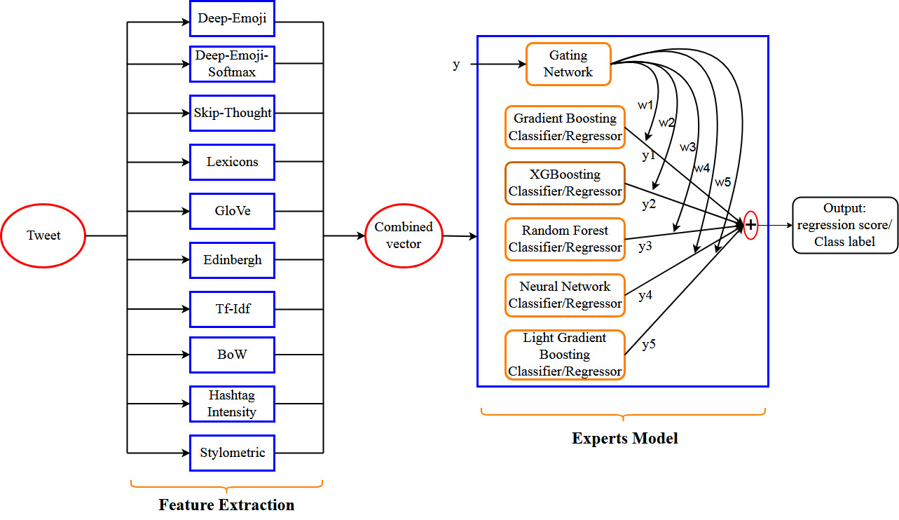
Figure 1: Proposed Experts model

4.2 Our Proposed Approach

We used the similar architecture, however with some modifications, to measure the intensity of an emotion in a tweet (regression) or predict an emotional intensity (classification). In our proposed approach, we pre-train each expert, to get parameters $\theta_{e}$, on the training samples, unlike traditional MoE model. Each expert, in itself, can be a separate Regression/Classification model like Multi-level Perceptron (MLP) model or Long Short-Term Memory (LSTM) model or any other model that best suits the data and task at hand. Once each expert is trained separately, we train only the gating network based on Gradient Descent Approach. The Detailed description of the model is depicted in Figure 1 and explained below.

We build different models - Neural Network Classifier/Regressor, Gradient Boosting Classifier/Regressor, XGBoost Classifier/Regressor, Random Forest Classifier/Regressor, Lasso Regressor and Light Gradient Boosting Classifier/Regressor and train each of them with the extracted feature vector of each tweet. We obtain this feature vector by concatenating all of the features discussed in Section 5. We assign parameters $\theta_{g}$, weights and bias, for each Classifier/Regressor at the gating network. Later, we train the gating network to fit the predicted $\hat{y}$ of each expert $i$ with actual $y$ and learn the best $\theta_{g}$.

Let $w[i]$ denote weight of each expert $i$ at the gating network. Let $b[i]$ denote the bias term for each expert $i$ at the gating network. Let $I$ be the number of experts. We define the Error function ($E$) as

$$E=\sum_{i=1}^{I}\frac{1}{2}prob[i]\Big{(}\mathbf{y}[i]-\hat{\mathbf{y}}[i]+b[i]\Big{)}^{2}$$

where $prob[i]$ is softmax probability of weight $w[i]$, $\mathbf{y}[i]$ is the actual $\mathbf{y}$ of $i^{th}$ expert for some sample $\mathbf{x}$. Similarly, $\hat{\mathbf{y}}[i]$ is the predicted $\mathbf{y}$ of $i^{th}$ expert for same sample $\mathbf{x}$. It is to be noted that $\forall i\hskip 3.0pt\mathbf{y}[i]=\mathbf{y}$.

For each sample $\mathbf{x}$ and $\mathbf{y}$, we train the gating network using the update equations of gradients as follows:

$$\frac{\partial E}{\partial w[i]} =\frac{1}{2}prob[i]\Big{(}1-prob[i]\Big{)}\Big{(}\mathbf{y}[i]-\hat{\mathbf{y}}[i]+b[i]\Big{)}^{2}$$

$$\frac{\partial E}{\partial b[i]} =prob[i]\Big{(}\mathbf{y}[i]-\hat{\mathbf{y}}[i]+b[i]\Big{)}$$

and

$$w[i] =w[i]-\eta*\frac{\partial E}{\partial w[i]}$$

$$b[i] =b[i]-\eta*\frac{\partial E}{\partial b[i]}$$

where $\eta$ is the learning rate.

5 Preprocessing & Feature Extraction

To preprocess each tweet, first we break all the contractions (like “can’t” to “cannot”, “I’m” to “I am” etc,.) followed by spelling corrections, decoding special words and acronyms (like “e g” to “eg”, “fb” to “facebook” etc,.) and symbol replacements (like “$” to “dollar”, “=” to “is equal to” etc). Later, we tokenized each tweet using NLTK tweet tokenizer .

The basic idea of using different experts and eclectic features is from the intuition that each expert learn from different aspects of the concatenated features. Hence, we explored and extracted a variety of features; and used only the features which best performs among all the explored ones are explained in the following subsections.

5.1 Deep-Emoji Features

Deep-Emoji [Felbo et al., 2017] performs prediction using the model trained on a dataset of 1246 million tweets and achieves state-of-the-art performance within sentiment, emotion and sarcasm detection. We can use the architecture of Deep-Emoji and train the model using millions of tweets from social media to get a better representation of new data. Using the pre-trained Deep-Emoji model, we extracted two different set of features - one, 64-dimensional vector from the softmax layer and the other, 2304-dimensional vector from attention layer.

5.2 Word-Embedding Features

In this paper, we tried four different pre-trained word-embedding approaches such as Word2Vec [Mikolov et al., 2013], GloVe [Pennington et al., 2014], Edinburgh Twitter Corpus [Petrović et al., 2010] and FastText [Bojanowski et al., 2017] for generating word vectors. We used the GloVe model of 300 dimensions.

5.3 Skip-Thought Features

Skip-Thoughts vectors [Kiros et al., 2015] model is in the framework of encoder-decoder models. Here, an encoder maps words to sentence vector and a decoder is used to generate the surrounding sentences. The main advantage of Skip-Thought vectors is that it can produce highly generic sentence representations from an encoder that share both semantic and syntactic properties of surrounding sentences. Here, we used Skip-Thought vector encoder model to produce a 4800 dimension vector representation of each tweet.

5.4 Lexicon Features

We also chose various lexicon features for the model. The lexicon features include AFINN Lexicon [Nielsen, 2011] (calculates positive and negative sentiment scores from the lexicon), MPQA Lexicon [Wilson et al., 2005] (calculates the number of positive and negative words from the lexicon), Bing Liu Lexicon [Bauman et al., 2017] (calculates the number of positive and negative words from the lexicon), NRC Affect Intensities, NRC-Word-Affect Emotion Lexicon, NRC Hash-tag Sentiment Lexicon, Sentiment140 Lexicon [Go et al., 2009] (calculates positive and negative sentiment score provided by the lexicon in which tweets are annotated by lexicons), and SentiWordNet [Baccianella et al., 2010] (calculates positive, negative, and neutral sentiment score). The final feature vector is the concatenation of all the individual features.

5.5 Hash-tag Intensity Features

The work by [Mohammad and Bravo-Marquez, 2017a] describes that removal of the emotion word hashtags causes the emotional intensity of the tweet to drop. This indicates that emotion word hashtags are not redundant with the rest of the tweet in terms of the overall intensity. Here, we used Depeche mood dictionary [Staiano and Guerini, 2014] to get the intensities of hashtag words. We average the intensities of all hashtags of a single tweet to get the total intensity score.

5.6 Stylometric Features

Tweets and other electronic messages (e-mails, posts, etc.) are written far shorter, way more informal and much richer in terms of expressive elements like emoticons and aspects at both syntax and structure level, etc. Common techniques use stylometric features [Anchiêta et al., 2015] which are categorized into 5 different types: lexical, syntactic, structural, content specific, and idiosyncratic. In this paper, we used 7 stylometric features such as “number of emoticons”, “number of nouns”, “number of adverbs”, “number of adjectives”, “number of punctuations”, “number of words”, and “average word length”.

5.7 Unsupervised Sentiment Neuron Features

Unsupervised sentiment neuron model [Radford et al., 2017] provides an excellent learning representation of sentiment, despite being trained only on the text of Amazon reviews. A linear model using this representation results in good accuracy. This model represents a 4096 feature vector for any given input tweet or text.

6 Experimental Setup & Results

To train our proposed approach, we consider a total of five learning models, one for each expert: Gradient Boosting, XGBoost, Light Gradient Boosting, Random Forest, and Neural Network(NN) for subtasks EI-reg and V-reg. While for the subtasks EI-oc and V-oc, we consider all the models except NN model. For subtask E-c, we consider all the models except Light Gradient Boosting model.

Model	Parameters
	n_estimators: 3000,
Gradient Boosting	Learning rate: 0.05
	Max_depth: 4
	n_estimators: 100
XGBoosting	learning_rate: 0.1
	max_depth: 3
	Optimizer: adam
Neural Network	Activation : relu
	n_estimators: 250
Random Forest	max_depth: 4
	n_estimators: 720
Light Gradient Boosting	learning_rate: 0.05
	num_leaves: 5

Table 2: Model-Parameters

	EI-reg (Pearson (all instances))					EI-reg (Pearson (gold in 0.5-1))
Team	macro-avg	anger	fear	joy	sadness	macro-avg	anger	fear	joy	sadness
SeerNet	0.799(1)	0.827	0.779	0.792	0.798	0.638(1)	0.708	0.608	0.708	0.608
NTUA-SLP	0.776(2)	0.782	0.758	0.771	0.792	0.610(2)	0.636	0.595	0.636	0.595
PlusEmo2Vec	0.766(3)	0.811	0.728	0.773	0.753	0.579(5)	0.663	0.497	0.663	0.497
psyML	0.765(4)	0.788	0.748	0.761	0.761	0.593(4)	0.657	0.541	0.657	0.541
Experts Model	0.753(5)	0.789	0.742	0.748	0.733	0.598(3)	0.656	0.582	0.546	0.608
Median Team	0.653(23)	0.654	0.672	0.648	0.635	0.490(23)	0.526	0.497	0.420	0.517
Baseline	0.520(37)	0.526	0.525	0.575	0.453	0.396(37)	0.455	0.302	0.476	0.350
Note : The numbers inside parenthesis in both macro-avg columns represent the rank

Table 3: Comparison of Regression results of various models with our Experts Model

	EI-oc (Pearson (all classes))					EI-oc (Pearson (some emotion))
Team	macro-avg	anger	fear	joy	sadness	macro-avg	anger	fear	joy	sadness
SeerNet	0.695(1)	0.706	0.637	0.720	0.717	0.547(1)	0.559	0.458	0.610	0.560
PlusEmo2Vec	0.659(2)	0.704	0.528	0.720	0.683	0.501(4)	0.548	0.320	0.604	0.533
psyML	0.653(3)	0.670	0.588	0.686	0.667	0.505(3)	0.517	0.468	0.570	0.463
Amobee	0.646(4)	0.667	0.536	0.705	0.673	0.480(5)	0.458	0.367	0.603	0.493
Experts Model	0.636(5)	0.658	0.576	0.666	0.644	0.520(2)	0.493	0.502	0.579	0.509
Median Team	0.530(17)	0.530	0.470	0.552	0.567	0.415(17)	0.408	0.310	0.494	0.448
Baseline	0.394(26)	0.382	0.355	0.469	0.370	0.296(26)	0.315	0.183	0.396	0.289
Note : The numbers inside parenthesis in both macro-avg columns represent the rank

Table 4: Comparison of Classification results of various models with our Experts Model

6.1 Training Strategy

At the input layer, we used a concatenation vector of all features: Deep-Emoji, Skip-Thought, Lexicons, Stylometric, BoW, Tf-IDF, Glove, Word2Vec, Edinburgh, and HashTagIntensity which is same for each expert. We combined both training and dev data and used them for training our model. The training model is validated by stratified K-fold approach in which the model is repeatedly trained on K-1 folds and the remaining one fold is used for validation.

In order to tune the hyper-parameters of our experts model, we adopt a grid search cross-validation for each learning model. Using grid search cross-validation, we set the various types of parameters based on the learning model. Table 2 shows the parameter settings for all experts.

6.2 Results

	V-reg (Pearson)
Team	(all instances)	(gold in 0.5-1)
SeerNet	0.873	0.697
TCS Research	0.861	0.680
PlusEmo2Vec	0.860	0.691
NTUA-SLP	0.851	0.688
Amobee	0.843	0.644
Experts Model	0.830	0.670
Median Team	0.784	0.509
Baseline	0.585	0.449

Table 5: Comparison of Valence-reg results of various models with our Experts Model

	V-oc (Pearson)
Team	(all instances)	(gold in 0.5-1)
SeerNet	0.836	0.884
PlusEmo2Vec	0.833	0.878
Amobee	0.813	0.865
psyML	0.802	0.869
EiTAKA	0.796	0.838
Experts Model	0.738	0.773
Median Team	0.682	0.754
Baseline	0.509	0.560

Table 6: Comparison of Valence-oc results of various models with our Experts Model

	E-c
Team	(acc.)	(micro F1)	(macro F1)
NTUA-SLP	0.588(1)	0.701	0.528
TCS Research	0.582(2)	0.693	0.530
PlusEmo2Vec	0.576(4)	0.692	0.497
psyML	0.574(5)	0.697	0.574
Experts Model	0.578(3)	0.691	0.581
Median Team	0.471(17)	0.599	0.464
Baseline	0.442(21)	0.570	0.443
Note : The numbers inside parenthesis in
accuracy column represent the rank

Table 7: Comparison of E-c results of various models with our Experts Model

To evaluate our computational model, we compare our results with SemEval-2018 Task-1 (Affect in Tweets) baseline results, top five performers and Median Team (as per SemEval-2018 results). The results in the EI-reg, EI-oc, V-reg, V-oc, E-c are shown in Tables 3, 4, 6, 6, 7 respectively. The tables illustrate (a) the results obtained by our proposed approach, (b) top five performers in SemEval-2018, (c) the results obtained by a baseline SVM system using unigrams as features and (d) Median Team among all submissions. From the Tables 3 and  4, we observe that our model (considering only macro-average for Pearson Correlation) for EI-reg and EI-oc stands within 5 places among 48 submissions. A quick walk-through of Table 3 for individual emotions shows that anger and fear ranks $3^{rd}$ and $4^{th}$ respectively for EI-reg Pearson(all instances) and for EI-reg Pearson(gold in 0.5-1), fear stands at $3^{rd}$ position and sadness equals score of top performer. Similarly, Table 4 for classification results shows that anger and fear ranks $4^{th}$ and $3^{rd}$ respectively for EI-oc Pearson(all classes) and for EI-oc Pearson(some emotion), anger, fear, joy and sadness stands at positions $4^{th}$, $1^{st}$, $4^{th}$ and $3^{rd}$ respectively. It is to be noted that in both Tables 3 and 4, the numbers inside parenthesis under column “macro-avg” represent the rank according to macro-avg Pearson scores. These values shows that our model stands at $3^{rd}$ and $2^{nd}$ positions in EI-reg Pearson(gold in 0.5-1) and EI-oc Pearson(some emotion) respectively. Tables 6 and 6 illustrate that the results from our model are among the top 10 submissions of subtasks V-reg and V-oc. Table 7 shows the results of multi-label emotion classification (11 classes). Our model is among the top 3 submissions for Jaccard similarity (accuracy) metric, in top 5 for micro F1 metric and topped the submissions for macro F1 metric.

6.3 Metrics

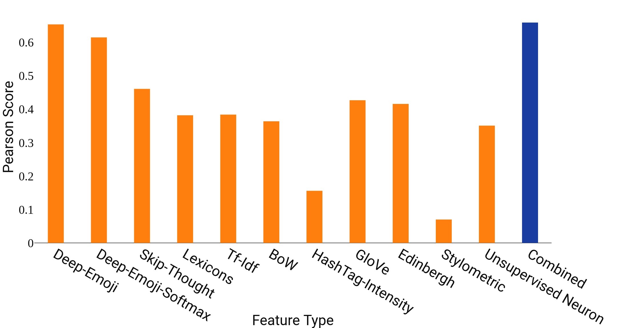
(a) Emotion: Anger

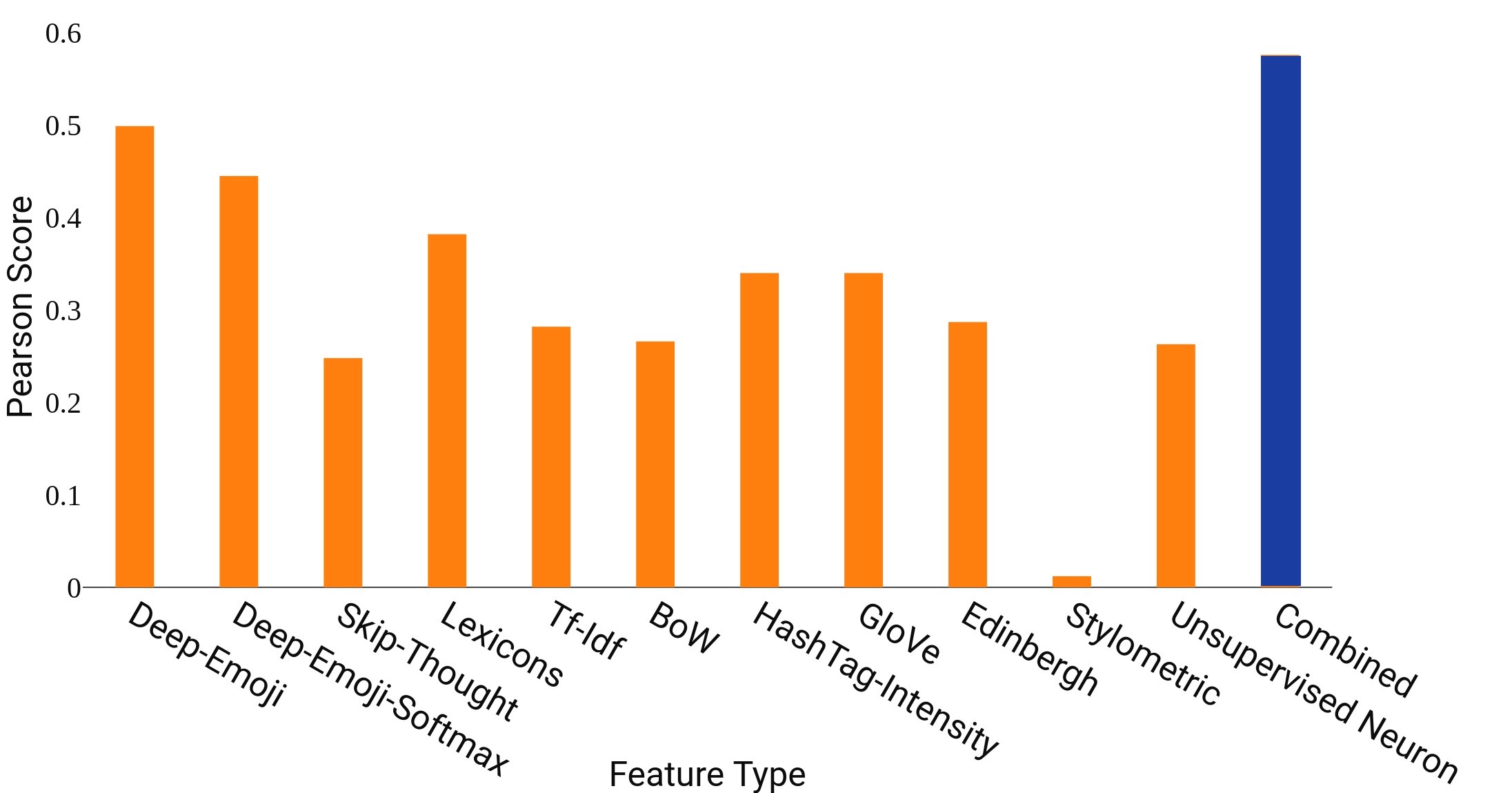
(b) Emotion: Fear

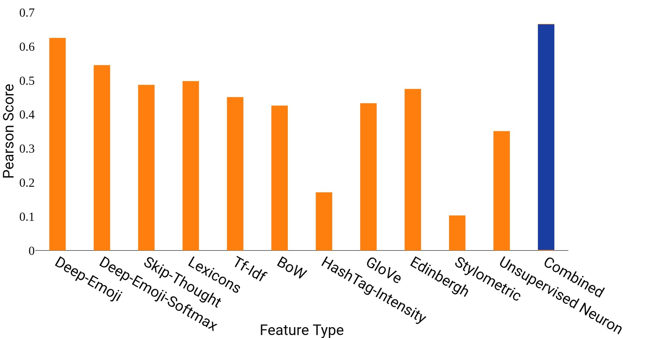
(c) Emotion: Joy

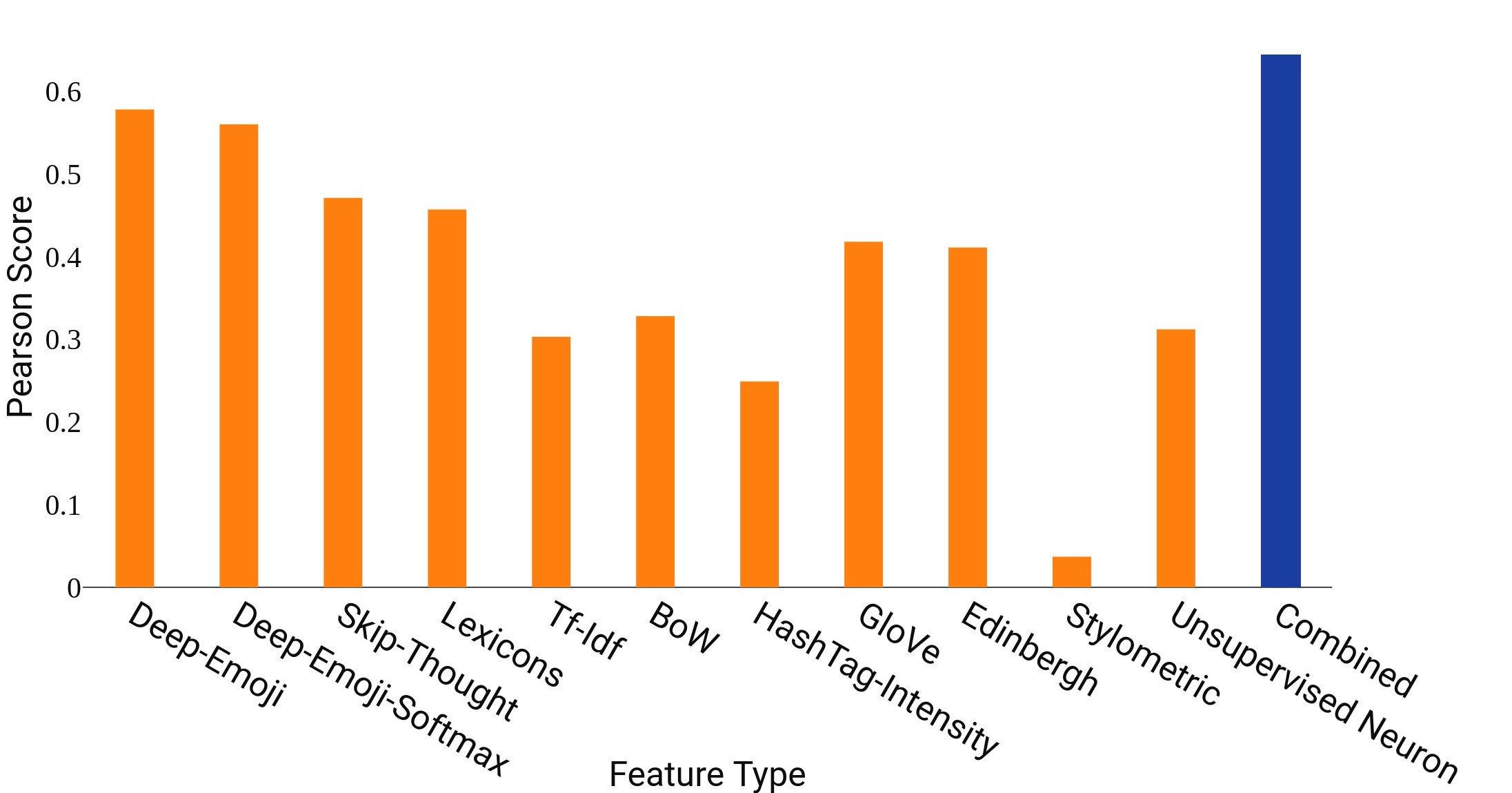
(d) Emotion: Sadness

Figure 2: Feature Importance: Comparison of Pearson Scores for each feature vector & concatenated vector

We use the competition metric, Pearson Correlation Coefficient with the Gold ratings/labels from SemEval-2018 task-1 AIT for EI-reg, EI-oc, V-reg and V-oc. Further, macro-average was calculated by averaging the correlation scores of four emotions: anger, fear, joy, and sadness for the tasks EI-reg and EI-oc. Along with Pearson Correlation Coefficient, we use some additional metrics for each subtask. The additional metric used for EI-reg and V-reg tasks was to calculate the Pearson correlation only for a subset of test samples where the intensity score was greater than or equal to 0.5. For the classification subtasks EI-oc and V-oc, we use the additional metric Pearson correlation calculated only for some emotion like low emotion, moderate emotion, or high emotion. However, for the multi label emotion classification E-c, we used the official evaluation metrics Jaccard Similarity (accuracy), micro average F1 score and macro average F1 score of all the classes.

Figure 2 shows the influence of each feature type on scores for predicting the intensity or emotion. We can observe from Figure 2 that for “Deep-Emoji” and “Deep-Emoji-Softmax” features, Pearson scores are dominating other feature types. Feature types - Skip-Thought, Lexicons, Glove, and Edinburgh features are contributing approximately similar in each of the 4 emotions. However, Stylometric features and features from Unsupervised sentiment neurons are performing worse.

7 Conclusion

In this paper, we have proposed a novel approach inspired from standard Mixture-of-Experts model to predict the intensity of an emotion(Regression) or level of an emotion (Classification) or multi-label emotion classification. Experiment results show that our proposed approach can effectively deal the emotion detection problem and stands at top-5 when compare with SemEval-2018 Task-1 AIT results and baseline results. As most of the Pearson scores are in the range of 0.50 to 0.75, there is a lot of scope for improvement in predicting emotions or quantifying the emotion intensity through various other approaches, which are yet to be unfolded. The source code is publicly available at https://goo.gl/NktJhF so that researchers and developers can work on this exciting problem collectively.

References

- [Anchiêta et al., 2015] Rafael T Anchiêta, Francisco Assis Ricarte Neto, Rogério Figueiredo de Sousa, and Raimundo Santos Moura. 2015. Using stylometric features for sentiment classification. In International Conference on Intelligent Text Processing and Computational Linguistics, pages 189–200. Springer.
- [Asur and Huberman, 2010] Sitaram Asur and Bernardo A Huberman. 2010. Predicting the future with social media. In Proceedings of the 2010 IEEE/WIC/ACM International Conference on Web Intelligence and Intelligent Agent Technology-Volume 01, pages 492–499. IEEE Computer Society.
- [Baccianella et al., 2010] Stefano Baccianella, Andrea Esuli, and Fabrizio Sebastiani. 2010. Sentiwordnet 3.0: an enhanced lexical resource for sentiment analysis and opinion mining. In Lrec, volume 10, pages 2200–2204.
- [Bauman et al., 2017] Konstantin Bauman, Bing Liu, and Alexander Tuzhilin. 2017. Aspect based recommendations: Recommending items with the most valuable aspects based on user reviews. In Proceedings of the 23rd ACM SIGKDD International Conference on Knowledge Discovery and Data Mining, pages 717–725. ACM.
- [Bojanowski et al., 2017] Piotr Bojanowski, Edouard Grave, Armand Joulin, and Tomas Mikolov. 2017. Enriching word vectors with subword information. Transactions of the Association for Computational Linguistics, 5:135–146.
- [dos Santos and Gatti, 2014] Cicero dos Santos and Maira Gatti. 2014. Deep convolutional neural networks for sentiment analysis of short texts. In Proceedings of COLING 2014, the 25th International Conference on Computational Linguistics: Technical Papers, pages 69–78.
- [Duppada and Hiray, 2017] Venkatesh Duppada and Sushant Hiray. 2017. Seernet at emoint-2017: Tweet emotion intensity estimator. arXiv preprint arXiv:1708.06185.
- [Duppada et al., 2018] Venkatesh Duppada, Royal Jain, and Sushant Hiray. 2018. Seernet at semeval-2018 task 1: Domain adaptation for affect in tweets. In Proceedings of The 12th International Workshop on Semantic Evaluation, SemEval@NAACL-HLT, New Orleans, Louisiana, June 5-6, 2018, pages 18–23.
- [Felbo et al., 2017] Bjarke Felbo, Alan Mislove, Anders Søgaard, Iyad Rahwan, and Sune Lehmann. 2017. Using millions of emoji occurrences to learn any-domain representations for detecting sentiment, emotion and sarcasm. In Proceedings of the 2017 Conference on Empirical Methods in Natural Language Processing, pages 1615–1625.
- [Go et al., 2009] Alec Go, Richa Bhayani, and Lei Huang. 2009. Twitter sentiment classification using distant supervision. CS224N Project Report, Stanford, 1(12).
- [Goel et al., 2017] Pranav Goel, Devang Kulshreshtha, Prayas Jain, and Kaushal Kumar Shukla. 2017. Prayas at emoint 2017: An ensemble of deep neural architectures for emotion intensity prediction in tweets. In Proceedings of the 8th Workshop on Computational Approaches to Subjectivity, Sentiment and Social Media Analysis, pages 58–65.
- [Jacobs et al., 1991] Robert A Jacobs, Michael I Jordan, Steven J Nowlan, and Geoffrey E Hinton. 1991. Adaptive mixtures of local experts. Neural Computation, 3(1):79–87.
- [Jin et al., 2007] Xin Jin, Ying Li, Teresa Mah, and Jie Tong. 2007. Sensitive webpage classification for content advertising. In Proceedings of the 1st International Workshop on Data Mining and Audience Intelligence for Advertising, pages 28–33. ACM.
- [Jordan and Jacobs, 1994] Michael I Jordan and Robert A Jacobs. 1994. Hierarchical mixtures of experts and the em algorithm. Neural Computation, 6(2):181–214.
- [Jordan and Xu, 1995] Michael I Jordan and Lei Xu. 1995. Convergence results for the em approach to mixtures of experts architectures. Neural Networks, 8(9):1409–1431.
- [Kiros et al., 2015] Ryan Kiros, Yukun Zhu, Ruslan R Salakhutdinov, Richard Zemel, Raquel Urtasun, Antonio Torralba, and Sanja Fidler. 2015. Skip-thought vectors. In Advances in Neural Information Processing Systems, pages 3294–3302.
- [Köper et al., 2017] Maximilian Köper, Evgeny Kim, and Roman Klinger. 2017. Ims at emoint-2017: emotion intensity prediction with affective norms, automatically extended resources and deep learning. In Proceedings of the 8th Workshop on Computational Approaches to Subjectivity, Sentiment and Social Media Analysis, pages 50–57.
- [Liu and Zhang, 2012] Bing Liu and Lei Zhang. 2012. A survey of opinion mining and sentiment analysis. In Mining Text Data, pages 415–463. Springer.
- [Marsella et al., 2010] Stacy Marsella, Jonathan Gratch, Paolo Petta, et al. 2010. Computational models of emotion. A Blueprint for Affective Computing-A Sourcebook and Manual, 11(1):21–46.
- [Mikolov et al., 2013] Tomas Mikolov, Ilya Sutskever, Kai Chen, Greg S Corrado, and Jeff Dean. 2013. Distributed representations of words and phrases and their compositionality. In Advances in Neural Information Processing Systems, pages 3111–3119.
- [Mohammad and Bravo-Marquez, 2017a] Saif Mohammad and Felipe Bravo-Marquez. 2017a. Emotion intensities in tweets. In Proceedings of the 6th Joint Conference on Lexical and Computational Semantics (* SEM 2017), pages 65–77.
- [Mohammad and Bravo-Marquez, 2017b] Saif Mohammad and Felipe Bravo-Marquez. 2017b. Wassa-2017 shared task on emotion intensity. In Proceedings of the 8th Workshop on Computational Approaches to Subjectivity, Sentiment and Social Media Analysis, pages 34–49. Association for Computational Linguistics.
- [Mohammad and Kiritchenko, 2015] Saif M Mohammad and Svetlana Kiritchenko. 2015. Using hashtags to capture fine emotion categories from tweets. Computational Intelligence, 31(2):301–326.
- [Mohammad et al., 2018] Saif M. Mohammad, Felipe Bravo-Marquez, Mohammad Salameh, and Svetlana Kiritchenko. 2018. Semeval-2018 Task 1: Affect in tweets. In Proceedings of International Workshop on Semantic Evaluation (SemEval-2018), New Orleans, LA, USA.
- [Mohammad, 2016] Saif M Mohammad. 2016. Sentiment analysis: Detecting valence, emotions, and other affectual states from text. In Emotion Measurement, pages 201–237. Elsevier.
- [Nielsen, 2011] Finn Årup Nielsen. 2011. A new anew: Evaluation of a word list for sentiment analysis in microblogs. arXiv preprint arXiv:1103.2903.
- [Nowlan and Hinton, 1991] Steven J Nowlan and Geoffrey E Hinton. 1991. Evaluation of adaptive mixtures of competing experts. In Advances in Neural Information Processing Systems, pages 774–780.
- [Paltoglou et al., 2010] Georgios Paltoglou, Mike Thelwall, and Kevan Buckley. 2010. Online textual communications annotated with grades of emotion strength. In Proceedings of the 3rd International Workshop of Emotion: Corpora for research on Emotion and Affect, pages 25–31.
- [Pang et al., 2008] Bo Pang, Lillian Lee, et al. 2008. Opinion mining and sentiment analysis. Foundations and Trends® in Information Retrieval, 2(1–2):1–135.
- [Pennington et al., 2014] Jeffrey Pennington, Richard Socher, and Christopher D. Manning. 2014. Glove: Global vectors for word representation. In Empirical Methods in Natural Language Processing (EMNLP), pages 1532–1543.
- [Petrović et al., 2010] Saša Petrović, Miles Osborne, and Victor Lavrenko. 2010. The edinburgh twitter corpus. In Proceedings of the NAACL HLT 2010 Workshop on Computational Linguistics in a World of Social Media, pages 25–26.
- [Qiu et al., 2010] Guang Qiu, Xiaofei He, Feng Zhang, Yuan Shi, Jiajun Bu, and Chun Chen. 2010. Dasa: dissatisfaction-oriented advertising based on sentiment analysis. Expert Systems with Applications, 37(9):6182–6191.
- [Radford et al., 2017] Alec Radford, Rafal Jozefowicz, and Ilya Sutskever. 2017. Learning to generate reviews and discovering sentiment. arXiv preprint arXiv:1704.01444.
- [Somasundaran et al., 2007] Swapna Somasundaran, Theresa Wilson, and Janyce Wiebe. 2007. Qa with attitude: Exploiting opinion type analysis for improving question answering in on-line discussions and the news. In ICWSM.
- [Staiano and Guerini, 2014] Jacopo Staiano and Marco Guerini. 2014. Depeche mood: a lexicon for emotion analysis from crowd annotated news. In Proceedings of the 52nd Annual Meeting of the Association for Computational Linguistics (Volume 2: Short Papers), volume 2, pages 427–433.
- [Stelmack and Stalikas, 1991] Robert M Stelmack and Anastasios Stalikas. 1991. Galen and the humour theory of temperament. Personality and Individual Differences, 12(3):255–263.
- [Stoyanov et al., 2005] Veselin Stoyanov, Claire Cardie, and Janyce Wiebe. 2005. Multi-perspective question answering using the opqa corpus. In Proceedings of the Conference on Human Language Technology and Empirical Methods in Natural Language Processing, pages 923–930. Association for Computational Linguistics.
- [Warriner et al., 2013] Amy Beth Warriner, Victor Kuperman, and Marc Brysbaert. 2013. Norms of valence, arousal, and dominance for 13,915 english lemmas. Behavior Research Methods, 45(4):1191–1207.
- [Wilson et al., 2004] Theresa Wilson, Janyce Wiebe, and Rebecca Hwa. 2004. Just how mad are you? finding strong and weak opinion clauses. In Proceedings of the 19th National Conference on Artifical intelligence, pages 761–767.
- [Wilson et al., 2005] Theresa Wilson, Janyce Wiebe, and Paul Hoffmann. 2005. Recognizing contextual polarity in phrase-level sentiment analysis. In Proceedings of the Conference on Human Language Technology and Empirical Methods in Natural Language Processing, pages 347–354. Association for Computational Linguistics.
- [Yuksel et al., 2012] Seniha Esen Yuksel, Joseph N Wilson, and Paul D Gader. 2012. Twenty years of mixture of experts. IEEE Transactions on Neural Networks and Learning Systems, 23(8):1177–1193.