Leading exponential finite size corrections for non-diagonal form factors

Abstract

We derive the leading exponential finite volume corrections in two dimensional integrable models for non-diagonal form factors in diagonally scattering theories. These formulas are expressed in terms of the infinite volume form factors and scattering matrices. If the particles are bound states then the leading exponential finite-size corrections ($\mu$-terms) are related to virtual processes in which the particles disintegrate into their constituents. For non-bound state particles the leading exponential finite-size corrections (F-terms) come from virtual particles traveling around the finite world. In these F-terms a specifically regulated infinite volume form factor is integrated for the momenta of the virtual particles. The F-term is also present for bound states and the $\mu$-term can be obtained by taking an appropriate residue of the F-term integral. We check our results numerically in the Lee-Yang and sinh-Gordon models based on newly developed Hamiltonian truncations.

1 Introduction

Two dimensional integrable quantum field theories are hoped to be exactly soluble. Theoretically, solvability allows us to find exact values for all physical observables including the energy spectrum and correlation functions at any finite size. However, even in integrable theories this very progressive task has not been completed yet. Integrability has only offered us a systematic way to attack these problems so far.

The first step of this systematic solution is to solve the theory in infinite volume by completing the S-matrix and form factor (FF) bootstraps [1, 2, 3, 4]. In infinite volume the powerful crossing symmetry can be used to derive restrictive functional relations for the scattering matrix and for the matrix elements of local operators, i.e. for form factors. Having solved these functional relations the resulting S-matrix and FFs can be used to describe all the finite size corrections systematically as follows.

At finite size, the leading corrections are polynomial in the inverse of the volume and originate from finite volume momentum quantization [5, 6]. Periodicity of the wave function requires that the scattering phase cancels the translational phase when a particle is moved around the cylinder and scattered through all other particles. The leading exponential corrections for bound states (called $\mu$-terms) are related to the fact that in a finite volume bound states can virtually decay into their constituents. The next exponential corrections (F-terms) are caused by the polarization of the non-trivial finite volume vacuum [7]. Pairs of virtual particles can appear from the vacuum. These travel around the world and scatter on the physical particles, then annihilate each other or get absorbed by the operators, such that this amplitude is described by the infinite volume form factor. There could be any number of virtual particles, which can also scatter on themselves. Thus, for an exact description all these virtual processes have to be quantified and summed up.

For the finite volume energy levels the momentum quantization is given by the so-called Bethe-Yang equations [5, 6], which provide the polynomial corrections. Leading exponential corrections for standing one-particle states were identified in [7] and were later extended for a single moving particle in [8, 9]. The contribution of a single pair of virtual particles was extended for multiparticle states in [10], while the similar contribution with two pairs of virtual particles was analyzed for the vacuum in [11], and for multiparticle states in [12]. Finally, all virtual processes are summed up by the Thermodynamic Bethe Ansatz (TBA) equation, which was derived in the simplest case in [6]. This provides the exact finite volume ground state energy. Excited states can be obtained by careful analytic continuations [13, 14].

For finite volume form factors our understanding is much more restricted. As far as polynomial corrections are concerned one merely has to take into account momentum quantization and the corresponding change in the normalization of states, which was proved for non-diagonal form factors in [15]. For diagonal form factors extra disconnected terms appear [16], which can be derived by carefully evaluating the diagonal limit of a non-diagonal form factor [17]. The finite volume one-point functions can be expressed in terms of the infinite volume connected form factors and the TBA pseudo energies [18, 19] in a way summing up the contributions of virtual processes. This result has been extended by analytic continuation for diagonal matrix elements in diagonally scattering theories [20, 21, 22]. The expansion of these formulae provides the leading exponential corrections for diagonal form factors. For non-diagonal form factors, however, even these leading exponential corrections are not known in general. For the simplest non-diagonal form factor (vacuum-one-particle state) the leading exponential $\mu$-term corrections were obtained in [23], while the $F$-term correction in [24]. The aim of the present paper is to extend these analyses for generic non-diagonal matrix elements in diagonally scattering theories. Although the $F$-term calculation was based on the form factor expansion of the torus two-point function [24], this method is very difficult to generalize even considering the interesting developments in [25, 26]. We thus focus on a formal and direct derivation of the cylinder one-point function in the crossed channel. We test the conjectured results by comparing them to the $\mu$-term corrections and to numerical data obtained from the combination of the Truncated Conformal Space Approach (TCSA) and mini-superspace approaches newly developed for the sinh-Gordon theory and from TCSA in the Lee-Yang model.

Our results provide the leading exponential corrections for form factors, which contribute to the leading exponential correction to correlation functions, too. These results can be relevant for various branches of physics including finite temperature and finite volume correlation functions in statistical and solid state systems as well as in lattice gauge theories, where the size of the system is inherently finite and finite size effects are unavoidable. Our results can be useful in the AdS/CFT correspondence, too, where the calculation of correlation functions boils down to the calculation of finite volume form factors of nonlocal operators [27] or, alternatively, it can be obtained by gluing hexagon [28] and octagon [29] amplitudes. This gluing procedure is analogous to the calculation of finite size effects of form factors and requires a regularization procedure [30]. Thus, our systematic method which gives rise to a regulated form factor could be implemented there as well.

The paper is organized as follows: In Section 2 we review the exact results for the finite size corrections of the energy spectrum. We start this by describing the existing excited state TBA equations for the sinh-Gordon and Lee-Yang models and expanding them iteratively to second order. We extract the $\mu$- and $F$-term corrections and demonstrate how the $\mu$- terms can be obtained from the $F$-terms by calculating appropriate residues. Section 3 deals with the finite size corrections of non-diagonal form factors. We first review the asymptotic results for polynomial corrections. Assuming the particles are bound states the asymptotic results provide the $\mu$-term corrections, which we derive in a compact form. Afterwards, we provide a formal derivation of the F-term corrections, relating them to the $\mu$-terms subsequently. In Section 4 we check numerically our formulas in the sinh-Gordon and Lee-Yang models and conclude in Section 5. Technical details are relegated to the Appendices.

2 Finite volume energy spectrum

In this section we recall how the TBA equations provide an exact description of the energy spectrum. We focus on theories with diagonal scatterings.

In the simplest case the theory has a single particle with mass $m$. Multiparticle scatterings factorize into the product of two-particle scatterings, with S-matrix $S(\theta)$, which satisfies unitarity and crossing symmetry

$$S(-\theta)=S^{-1}(\theta)\quad;\qquad S(i\pi-\theta)=S(\theta)$$ (2.1)

Here $\theta$ is the rapidity difference of the particles $\theta=\theta_{1}-\theta_{2}$. The simplest non-trivial scattering matrix is

$$S(\theta)=\frac{\sinh\theta-i\sin p\pi}{\sinh\theta+i\sin p\pi}$$ (2.2)

For $p>0$ there is no singularity in the physical strip $\Im m(\theta)\in[0,\pi]$ and the scattering matrix corresponds to the sinh-Gordon theory. However, if $p<0$ bound states have to be introduced to explain the appearing poles. For $p=-\frac{2}{3}$ the scattering matrix

$$S(\theta)=\frac{\sinh\theta+i\sin\frac{\pi}{3}}{\sinh\theta-i\sin\frac{\pi}{3}}$$ (2.3)

satisfies the relation

$$S(\theta+iu)S(\theta-iu)=S(\theta)\quad;\qquad u=\frac{\pi}{3}$$ (2.4)

which, together with the bound state energy relation

$$m\cosh\theta=m\cosh(\theta+iu)+m\cosh(\theta-iu)$$ (2.5)

implies that the bound state is the original particle itself. This theory is a consistent scattering theory [31], called the scaling Lee-Yang model.

2.1 Sinh-Gordon finite size spectrum

The exact finite volume energy spectrum can be obtained by calculating the continuum limit of an integrable lattice regularization [32]. A finite volume multiparticle state can be described by the pseudo energy $\epsilon(\theta|\{\theta_{j}\})$ and parameters $\{\bar{\theta}_{j}\}_{j=1,\dots,N}$ satisfying the non-linear integral equation

$$\epsilon(\theta|\{\theta\})=mL\cosh\theta+\sum_{j}\log S(\theta-\theta_{j}-\frac{i\pi}{2})-\int_{-\infty}^{\infty}\frac{dv}{2\pi}\phi(\theta-v)\log(1+e^{-\epsilon(v|\{\theta\})})$$ (2.6)

where $\phi(\theta)=-i\partial_{\theta}\log S(\theta)$ and the particles’ rapidities satisfy the quantization condition

$$Q_{k}(\{\bar{\theta}\})=2\pi n_{k}\qquad;\qquad Q_{k}(\{\theta\})=-i\epsilon(\theta_{k}+\frac{i\pi}{2}|\{\theta\})-\pi\quad;\qquad k=1,\dots,N$$ (2.7)

Here and from now on we abbreviate the set of rapidities $\{\theta_{j}\}_{j=1,\dots,N}$ as $\{\theta\}$. Given quantization numbers $n_{k}$, the rapidities $\{\bar{\theta}\}$ and the pseudo energy $\epsilon(\theta|\{\bar{\theta}\})$ can be determined, which provide the finite volume energy of the multiparticle state via

$$E_{\{n\}}(L)=m\sum_{j}\cosh\bar{\theta}_{j}-m\int_{-\infty}^{\infty}\frac{dv}{2\pi}\,\cosh v\,\log(1+e^{-\epsilon(v|\{\bar{\theta}\})})$$ (2.8)

We note that both in(2.6) and (2.8) the terms with the sum can be absorbed into the integral term by choosing a contour which goes around the singularities of the integrands at $v=\bar{\theta}_{j}+i\frac{\pi}{2}$. These zero of logarithm singularities are actually encoded in the quantization conditions (2.7).

2.1.1 Polynomial energy corrections

The TBA equations admit a systematic large volume expansion. At leading order, indicated by a superscript $(0)$, we drop the exponentially small integral terms and arrive at

$$\epsilon^{(0)}(\theta|\{\theta\})=mL\cosh\theta+\sum_{j}\log S(\theta-\theta_{j}-\frac{i\pi}{2})$$ (2.9)

Asymptotic rapidities satisfy the Bethe-Yang equations

$$Q_{k}^{(0)}(\{\bar{\theta}^{(0)}\})=2\pi n_{k}\quad;\qquad Q_{k}^{(0)}(\{\theta\})=mL\sinh\theta_{k}-i\sum_{j:j\neq k}\log S(\theta_{k,j})$$ (2.10)

where $\theta_{k,j}=\theta_{k}-\theta_{j}$. This equation has a very transparent meaning. Periodicity of the multiparticle wavefunction requires that, when moving particle $k$ around the circle, the acquired phase – consisting of the translational and the scattering phases – has to be a multiple of $2\pi$.

The energy at leading order is simply the sum of the one-particle energies

$$E_{\{n\}}^{(0)}(L)=m\sum_{j}\cosh\bar{\theta}_{j}^{(0)}$$ (2.11)

incorporating all finite volume corrections, which are polynomial in the inverse of the volume.

2.1.2 Leading exponential volume corrections

The leading exponential volume correction can be obtained by iterating the exact equations once. At this order, denoted by superscript $(1)$, we have

$$\epsilon^{(1)}(\theta|\{\theta\})=mL\cosh\theta+\sum_{i}\log S(\theta-\theta_{i}-\frac{i\pi}{2})-\int_{-\infty}^{\infty}\frac{dv}{2\pi}\phi(\theta-v)e^{-\epsilon^{(0)}(v|\{\theta\})}$$ (2.12)

and the quantization conditions get modified as

$$Q_{k}^{(1)}(\{\bar{\theta}^{(1)}\})=2\pi n_{k}\quad;\qquad Q_{k}^{(1)}(\{\theta\})=Q_{k}^{(0)}(\{\theta\})+\partial_{k}\Phi(\{\theta\})$$ (2.13)

where $\partial_{i}\equiv\partial_{\theta_{i}}\equiv\frac{\partial}{\partial\theta_{i}}$ and

$$\Phi(\{\theta\})=\int_{-\infty}^{\infty}\frac{dv}{2\pi}\prod_{j}S(v+i\frac{\pi}{2}-\theta_{j})e^{-mL\cosh v}$$ (2.14)

The exponentially corrected energy is

$$E_{\{n\}}^{(1)}(L)=m\sum_{i}\cosh\bar{\theta}_{i}^{(1)}-m\int_{-\infty}^{\infty}\frac{dv}{2\pi}\,\cosh v\,\prod_{j}S(v+i\frac{\pi}{2}-\bar{\theta}_{j}^{(0)})e^{-mL\cosh v}$$ (2.15)

which can be expressed also in terms of $\bar{\theta}_{i}^{(0)}$ as in [10]. The integral terms in all formulae above are called the $F$-term corrections.

2.2 Scaling Lee-Yang finite size spectrum

The ground state TBA equation was derived in [6], and careful analytical continuation in the volume lead to the TBA equations of excited states [13]. The same TBA equations can be derived from a continuum limit of a lattice model as well [33]. The TBA equations are formally the same as in the sinh-Gordon theory except that each particle with rapidity $\bar{\theta}_{j}$ is represented as a bound state of two ’elementary’ particles of rapidities $\bar{\theta}_{j\pm}=\bar{\theta}_{j}\pm i\bar{u}_{j}$. Thus, the pseudo energy equations are

$$\epsilon(\theta|\{\theta_{\pm}\})=mL\cosh\theta+\sum_{j,s=\pm}\log S(\theta-\theta_{js}-\frac{i\pi}{2})-\int_{-\infty}^{\infty}\frac{dv}{2\pi}\phi(\theta-v)\log(1+e^{-\epsilon(v|\{\theta_{\pm}\})})$$ (2.16)

where $\{\theta_{\pm}\}$ is the shorthand for $\{\theta_{j\pm}\}$ and the quantization conditions are

$$Q_{k\pm}(\{\bar{\theta}_{\pm}\})=2\pi n_{k\pm}\quad;\qquad Q_{k\pm}(\{\theta_{\pm}\})=-i\epsilon(\theta_{k\pm}+\frac{i\pi}{2}|\{\theta_{\pm}\})-\pi\quad;\qquad k=1,\dots,N$$ (2.17)

It is advantageous to introduce the symmetric and antisymmetric combinations of these equations

$$Q_{k}(\{\theta_{\pm}\})=Q_{k+}(\{\theta_{\pm}\})+Q_{k-}(\{\theta_{\pm}\})\quad;\qquad\bar{Q}_{k}(\{\theta_{\pm}\})=Q_{k+}(\{\theta_{\pm}\})-Q_{k-}(\{\theta_{\pm}\})$$ (2.18)

The energy formula is also analogous to the sinh-Gordon theory:

$$E_{\{n_{\pm}\}}(L)=m\sum_{js}\cosh\bar{\theta}_{js}-m\int_{-\infty}^{\infty}\frac{dv}{2\pi}\,\cosh v\,\log(1+e^{-\epsilon(v|\{\bar{\theta}_{\pm}\})})$$ (2.19)

2.2.1 Polynomial and $\mu$-term energy corrections

Let us expand the equations as before by dropping the integral terms. We indicate this order by a superscript $(\mu)$ on $\bar{\theta}_{j\pm}^{(\mu)}=\bar{\theta}_{j}^{(\mu)}\pm i\bar{u}_{j}^{(\mu)}$ as it contains both polynomially and exponentially small volume corrections. Similarly to the sinh-Gordon case we assign the superscript $(0)$ for polynomial corrections only. The pseudo energy at this order is:

$$\epsilon^{(0)}(\theta|\{\theta_{\pm}\})=mL\cosh\theta+\sum_{js}\log S(\theta-\theta_{js}-\frac{i\pi}{2})$$ (2.20)

while the BY equations read as $Q_{k\pm}^{(0)}(\{\bar{\theta}_{\pm}^{(\mu)}\})=2\pi n_{k\pm}$ with

$$Q_{k\pm}^{(0)}(\{\theta_{\pm}\})=mL\sinh(\theta_{k\pm})-i\log S(\theta_{k\pm,k\mp})-i\sum_{j:j\neq k,s}\log S(\theta_{k\pm,js})$$ (2.21)

Focusing on the imaginary part of the equations we see that in the $L\to\infty$ limit the term $imL\cosh\bar{\theta}_{j}^{(\mu)}\sin\bar{u}_{j}^{(\mu)}$ goes to $i\infty$. This can be compensated only by the bound state pole of the scattering matrix

$$S(\theta)=i\frac{\Gamma^{2}}{\theta-2iu}+S_{0}+O(\theta-2iu),\quad\Gamma^{2}=-2\sqrt{3}$$ (2.22)

which forces $\bar{u}_{j}$ to approach $u$ in the large volume limit. Let us parametrize $\bar{u}_{j}^{(\mu)}$ as

$$\bar{u}_{j}^{(\mu)}=u+\delta\bar{u}_{j}$$ (2.23)

The relation $S(2i\bar{u}_{j}^{(\mu)})=\frac{\Gamma^{2}}{2\delta\bar{u}_{j}}+\dots$ together with (2.21) imply that $\delta\bar{u}_{j}$ is actually exponentially small in the volume. We can then expand the equations for large volume in $\delta\bar{u}_{j}$.

At leading order we set $\delta\bar{u}_{j}$ to be zero, i.e. we keep only the polynomial corrections and take $\bar{\theta}_{j\pm}^{(0)}=\bar{\theta}_{j}^{(0)}\pm iu$. Using the fusion property of the scattering matrix one can see that $Q_{k}^{(0)}(\{\bar{\theta}_{\pm}^{(0)}\})=Q_{k}^{(0)}(\{\bar{\theta}^{(0)}\})$. The resulting formulas are exactly the same as the sinh-Gordon equations (2.9-2.11) with quantization numbers $n_{j}=n_{j+}+n_{j-}$.

At the leading non-vanishing order in $\delta\bar{u}_{k}$ the equation for $\bar{Q}_{k}^{(0)}(\{\bar{\theta}\})$ determines $\delta\bar{u}_{k}$ as

$$\delta\bar{u}_{k}=(-1)^{n_{k}}\frac{\Gamma^{2}}{2}e^{-mL\sin u\cosh\bar{\theta}_{k}^{(0)}}\prod_{j:j\neq k}\sqrt{\frac{S(\bar{\theta}_{k,j}^{(0)}+iu)}{S(\bar{\theta}_{k,j}^{(0)}-iu)}}$$ (2.24)

Clearly this expression is at least as small as $e^{-\mu L}$ with $\mu=m\sin u$ and that is why we only kept the polynomial corrections in the $\theta$s, using $\bar{\theta}_{j}^{(0)}$ here. Alternatively, we could determine $\delta\bar{u}_{k}$ from the expansion of the two equations for $Q_{k\pm}^{(0)}(\{\theta_{\pm}\})$. By introducing

$$\delta u_{k\pm}(\{\theta\})=\frac{\Gamma^{2}}{2}e^{\pm im_{a}L\sinh(\theta_{k}\pm iu)}\prod_{j:j\neq k}S(\theta_{k,j}\pm iu)^{\pm 1}$$ (2.25)

the solutions of the Bethe-Yang equations will be

$$\delta\bar{u}_{k}=\delta u_{k+}(\{\bar{\theta}^{(0)}\})=\delta u_{k-}(\{\bar{\theta}^{(0)}\})$$ (2.26)

Using these quantities the Bethe-Yang equations for $\bar{\theta}_{j}$ at first order in $\delta\bar{u}_{j}$, i.e. at order $(\mu)$, takes the form

$$Q_{j}^{(\mu)}(\{\bar{\theta}^{(\mu)}\})=2\pi n_{j}\quad;\qquad Q_{j}^{(\mu)}(\{\theta\})=Q_{j}^{(0)}(\{\theta\})+\partial_{j}\sum_{k}(\delta u_{k+}(\{\theta\})+\delta u_{k-}(\{\theta\}))$$ (2.27)

where we used that $\partial_{j}\delta u_{k\pm}(\{\theta\})=\pm i\delta u_{j\pm}(\{\theta\})\partial_{j}Q_{k\pm}^{(0)}(\{\theta\pm iu\})$ (and the bound state relations (2.4-2.5)).

Thus, dropping the integral terms in the TBA equations not only gives the polynomial corrections, but also provides the leading exponential $\mu$-term corrections. This can be seen in the energy formula as well, which at leading order reads as

$$E_{\{n\}}^{(\mu)}(L)=m\sum_{j,s}\cosh\bar{\theta}_{js}^{(\mu)}=m\sum_{j}\cosh\bar{\theta}_{j}^{(\mu)}-2m\sin u\sum_{j}\cosh\bar{\theta}_{j}^{(0)}\delta\bar{u}_{j}$$ (2.28)

We note that here $\bar{\theta}_{j}^{(\mu)}$ also contains exponentially small corrections coming form the quantization condition (2.27), which involves $\mu$-terms.

2.2.2 F-term energy correction

To iterate the integral equations once we use the leading order term in the integrand. These formulas are completely equivalent to (2.12-2.15) except that each rapidity comes in pairs, $\theta_{j\pm}$. These equations contain both the $O(e^{-mL})$ and $O(e^{-(\mu+m)L})$ corrections. In the following we are only interested in the $O(e^{-\mu L})$ and $O(e^{-mL})$ corrections thus we put $\delta u_{j}=0$ in the integrands. At this order, denoted by superscript $(1)$, we have

$$\epsilon^{(1)}(\theta|\{\theta\}) = mL\cosh\theta+\sum_{j}\log S(\theta-\theta_{j}-\frac{i\pi}{2})+\sum_{j}\phi(\theta-iu-\frac{i\pi}{2}-\theta_{j})\delta u_{j-}(\{\theta\})$$

$$-\sum_{j}\phi(\theta+iu-\frac{i\pi}{2}-\theta_{j})\delta u_{j+}(\{\theta\})-\int_{-\infty}^{\infty}\frac{dv}{2\pi}\phi(\theta-v)\prod_{j}S(v+i\frac{\pi}{2}-\theta_{j})e^{-mL\cosh(v)}$$

Since the quantization condition $\bar{Q}_{k}$ modifies $\delta u_{k}$ only at order $O(e^{-(m+\mu)L})$ we focus on $Q_{k}$. In addition to (2.27) we also get an integral term

$$Q_{k}^{(1)}(\{\bar{\theta}\})=2\pi n_{k\pm}\quad;\qquad Q_{k}^{(1)}(\{\theta\})=Q_{k}^{(0)}(\{\theta\})+\partial_{k}\sum_{j}(\delta u_{j+}(\{\theta\})+\delta u_{j-}(\{\theta\}))+\partial_{k}\Phi(\{\theta\})$$ (2.30)

where $\Phi(\{\theta\})$ is the same as (2.14). The exponentially corrected energy also gets the integral term

$$E_{\{n\}}^{(1)}(L)=m\sum_{j}\cosh\bar{\theta}_{j}^{(1)}-2m\sin u\sum_{j}\cosh\bar{\theta}_{j}^{(0)}\delta u_{j}-m\int_{-\infty}^{\infty}\frac{d\theta}{2\pi}\,\cosh\theta\,\prod_{j}S(\theta+i\frac{\pi}{2}-\bar{\theta}_{j}^{(0)})e^{-mL\cosh\theta}$$ (2.31)

In all the formulas (2.2.2,2.30,2.31) terms containing $\delta u_{j}$ are the $\mu$-terms, while the integral terms are the $F$-terms. Note that the $F$-terms are universal in the sense that they are the same for both theories once the corresponding S-matrix is used. It is also very important for our further study to point out that in the Lee-Yang theory the two corrections are not independent: the $\mu$ terms can be obtained as appropriate residues of the $F$-terms. Indeed, the scattering matrix not only has a pole at $\theta=2iu=i\frac{2\pi}{3}$ but also at $\theta=i\pi-2iu=i\frac{\pi}{3}$ with opposite residue. This implies that $e^{-\epsilon^{(0)}(\theta|\{\theta\})}$ has poles at $\theta=\theta_{j}\pm i\frac{\pi}{6}$ with residues

$$\text{Res}_{\theta=\theta_{j}\pm i\frac{\pi}{6}}e^{-\epsilon^{(0)}(\theta|\{\theta\})}=\pm 2i\delta u_{j\mp}(\{\theta\})$$ (2.32)

We can think of taking the real contour and deforming half of it onto the upper half-plane and the other half to the lower half-plane. Then we can subtract the two residues, which appear with opposite orientations. As a result we can recover the $\mu$-terms from the $F$-terms in all the formulas (2.2.2-2.31). Alternatively, we can choose the contours of integration as shown in Figure 1 and keep only the $F$-term integral, which is universal and is the same for both theories.

Figure 1: Integration contour, which contains both the $F$- and the $\mu$-terms.The integrand is half the $F$-term integrand both on the upper and on the lower contour.

3 Finite volume form factors

In this section we summarize the results for finite volume form factors. We start by reviewing the definition of these quantities together with the available results for the polynomial finite size corrections. We then derive the leading exponential $\mu$- and $F$-term corrections for general nondiagonal finite volume form factors. Technical details are presented in Appendices A and B. In Appendix C we also show how the $\mu$-term correction can be obtained from the $F$-term corrections.

Finite volume form factors are the matrix elements of local operators ${\cal O}(x,t)$ between finite volume energy eigenstates, which can be labeled either by the quantization numbers $\{n_{i}\}$ or by the corresponding rapidities $\{\bar{\theta}_{i}\}$:

$$|\bar{\theta}_{1},\dots,\bar{\theta}_{N}\rangle_{L}=|\{\bar{\theta}\}\rangle_{L}\equiv|n_{1},\dots,n_{N}\rangle_{L}=|\{n\}\rangle_{L}$$ (3.1)

These rapidities satisfy the exact quantization conditions (2.7) or the related equations for the Lee-Yang theory (2.17).

Our aim is to express the finite volume form factors in terms of the scattering matrix and the infinite volume elementary form factors defined by

$$\langle 0|{\cal O}(0,0)|\theta_{1},\dots,\theta_{N}\rangle=F_{N}^{{\cal O}}(\theta_{1},\dots,\theta_{N})$$ (3.2)

These infinite volume form factors satisfy the monodromy axioms:

$$F_{N}(\theta_{1},\dots,\theta_{N})=F_{N}(\theta_{2},\dots,\theta_{N},\theta_{1}-2i\pi)=S(\theta_{i,i+1})F_{N}(\theta_{1},\dots,\theta_{i+1},\theta_{i},\dots,\theta_{N})$$ (3.3)

which together with their known analytic properties allows one to find the relevant physical solutions.

Form factors have pole singularities, with either kinematical or dynamical origin. The kinematical pole is related to disconnected diagrams and appear whenever an outgoing particle coincides with an incoming one. At the level of the elementary form factor this implies that

$$F_{N+2}(\theta+i\pi+\frac{\epsilon}{2},\theta-\frac{\epsilon}{2},\{\theta\})=\frac{i}{\epsilon}(1-\prod_{j}S(\theta-\theta_{j}))F_{N}(\{\theta\})+F_{N+2}^{r}(\theta+i\pi,\theta,\{\theta\})+O(\epsilon)$$ (3.4)

where we introduced a specific symmetric evaluation, since the $O(1)$ piece defined this way, that we call the regulated form factor, will be relevant in the further discussions. The notation $\{\theta\}$ abbreviates the ordered set $\{\theta_{1},\dots,\theta_{N}\}$.

Dynamical pole singularities are only present for theories in which the scattering matrix has a bound state pole. They relate the form factors of elementary particles to those of bound states. For the Lee-Yang model they read as

$$F_{N+2}(\theta+iu+\frac{\epsilon}{2},\theta-iu-\frac{\epsilon}{2},\{\theta\})=\frac{i\Gamma}{\epsilon}F_{N+1}(\theta,\{\theta\})+F_{N+1}^{b}(\theta,\{\theta\})+O(\epsilon)$$ (3.5)

where the symmetrically evaluated $O(1)$ piece will be used later on. In particular, we will need the expansion

$$F_{2N}(\theta_{1}+iu+\frac{\epsilon_{1}}{2},\theta_{1}-iu-\frac{\epsilon_{1}}{2},\dots,\theta_{N}+iu+\frac{\epsilon_{N}}{2},\theta_{N}-iu-\frac{\epsilon_{N}}{2})=\,\,\,\,\,\,\,\,\,\,\,\,\,\,\,\,\,\,\,\,\,\,\,$$ (3.6)

$$\,\,\,\,\,\,\,\,\,\,\,\,\,\,\,\,\,\prod_{j}\left(\frac{i\Gamma}{\epsilon_{j}}\right)\left\{F_{N}(\{\theta\})-i\Gamma^{-1}\sum_{k}\epsilon_{k}F_{N,k}^{b}(\{\theta\})+O(\epsilon^{2})\right\}$$

In diagonally scattering theories with a single species the form factors take the form

$$F_{N}^{{\cal O}}(\theta_{1},\dots,\theta_{N})=H_{N}^{{\cal O}}\prod_{i<j}\frac{f(\theta_{i,j})}{x_{i}+x_{j}}P_{N}^{{\cal O}}(x_{1},\dots,x_{N})\quad;\qquad x_{i}=e^{\theta_{i}}$$ (3.7)

where $f(\theta)$ is the minimal two particle form factor, which satisfies $f(\theta)=S(\theta)f(-\theta)=f(2i\pi-\theta)$ and has the right dynamical pole. In the sinh-Gordon theory it does not have any singularity in the physical strip:

$$f(\theta)=\exp\left\{-4\int_{0}^{\infty}\frac{dx}{x}\frac{\sinh(\frac{xp}{2})\sinh(\frac{x}{2}(1-p))\sinh(\frac{x}{2})}{\sinh^{2}(x)}\cos\left(\frac{x}{\pi}(i\pi-\theta)\right)\right\}$$ (3.8)

while in the Lee-Yang theory it can be obtained by an analytic continuation of this:

$$f(\theta)=\frac{\cosh\theta-1}{\cosh\theta+\frac{1}{2}}\exp\left\{4\int_{0}^{\infty}\frac{dx}{x}\frac{\sinh(\frac{x}{2})\sinh(\frac{x}{3})\sinh(\frac{x}{6})}{\sinh^{2}(x)}\cos\left(\frac{x}{\pi}(i\pi-\theta)\right)\right\}$$ (3.9)

3.1 Polynomial finite volume corrections

Let us analyze the following finite volume form factor

$$\langle\bar{\vartheta}_{1},\dots,\bar{\vartheta}_{M}|\mathcal{O}|\bar{\theta}_{1},\dots,\bar{\theta}_{N}\rangle_{L}\equiv\langle\{\bar{\vartheta}\}|\mathcal{O}|\{\bar{\theta}\}\rangle_{L}$$ (3.10)

As far as polynomial corrections are concerned the rapidities $\{\bar{\theta}_{i}\}$ satisfy the Bethe-Yang equations (2.10) and there are analogous equations for $\vartheta$s with quantization numbers $m_{k}$. As it was shown in [15] the polynomial finite volume corrections of form factors solely come from the normalization change of the finite volume states. These states are normalized to Kronecker delta functions, while infinite volume states are normalized to Dirac delta functions. Additionally, the phase of finite volume states is usually chosen such that it is symmetric for the exchanges of rapidities, as opposed to the phase of infinite volume states, which pick up the scattering matrix whenever two neighboring particles are exchanged (3.3). Thus, the finite volume form factor at order $(0)$ is

$$\langle\{m\}|\mathcal{O}|\{n\}\rangle_{L}=\frac{F_{N+M}(\{\bar{\vartheta}^{(0)}+i\pi\},\{\bar{\theta}^{(0)}\})}{\sqrt{\prod_{i<j}S(\bar{\vartheta}_{j,i}^{(0)})\rho_{M}^{(0)}(\{\bar{\vartheta}^{(0)}\})\prod_{i<j}S(\bar{\theta}_{i,j}^{(0)})\rho_{N}^{(0)}(\{\bar{\theta}^{(0)}\})}}$$ (3.11)

where the density of states $\rho_{N}^{(0)}(\{\bar{\theta}^{(0)}\})$ is defined as the determinant of the matrix $\partial_{i}Q_{j}^{(0)}(\{\theta\})$:

$$\rho_{N}^{(0)}(\{\theta\})=\det\left|\partial_{j}Q_{i}^{(0)}(\{\theta\})\right|$$ (3.12)

which is the Jacobian for changing the variables from $\{n\}$ to $\{\bar{\theta}^{(0)}\}$ via $Q_{k}^{(0)}(\bar{\theta}_{j}^{(0)})=2\pi n_{k}$. This form for the polynomial finite size corrections is correct only if the matrix element is non-diagonal, i.e. if the quantum numbers $\{n\}$ and $\{m\}$ are not exactly the same. For diagonal form factors a more complicated formula is valid including disconnected terms [16], which can be obtained from the non-diagonal form factor by taking an appropriate limit [17]. Expression (3.11) contains all polynomial corrections in the inverse of the volume and is valid for any theory with a single particle type, in particular, for both the sinh-Gordon and the scaling Lee-Yang models.

3.2 Leading exponential corrections: the $\mu$-term

In this subsection we calculate the $\mu$-terms for finite volume form factors in the scaling Lee-Yang model. This is analogous to the order $(\mu)$ calculation of the energy in subsubsection 2.2.1. As we have shown there the results at this order can be obtained by taking the order $(0)$ correction with the additional requirement that each particle is a bound state represented by its constituents. Expanding the bound states’ equations to the leading exponential order provided the $\mu$-terms for the energy. Based on this observation Pozsgay suggested in [23] that the $\mu$-terms for form factors can be calculated by taking the form (3.11) with the additional assumption that each particle with rapidity $\bar{\theta}_{j}$ is represented as a bound state of particles with rapidities $\bar{\theta}_{j\pm}$. He also carried out this calculation for the simplest one-particle form factor $\langle 0|\mathcal{O}|\theta\rangle_{L}$ and checked the results numerically with the TCSA method. In the following we calculate the $\mu$-term correction for a generic $N$-particle state based on this idea.

We start with the order $\left(0\right)$ form factor in which only incoming particles are present, composed from the constituents $\theta_{j\pm}$:

$$\langle 0|\mathcal{O}|\{\theta_{\pm}\}\rangle_{L}=\frac{F_{2N}(\theta_{1+},\theta_{1-},\ldots\theta_{N+},\theta_{N-})}{\sqrt{\prod\limits_{k}S(\theta_{k+,k-})\rho_{2N}(\{\theta_{\pm}\})\prod\limits_{i<j,r,s}S(\theta_{ir,js})}}$$ (3.13)

We evaluate this expression at $\theta_{j\pm}=\bar{\theta}_{j\pm}^{(\mu)}=\bar{\theta}_{j}^{(\mu)}\pm i(u+\delta\bar{u}_{j})$ and expand to leading order in $\delta\bar{u}_{j}$. Since at the leading order both the numerator and the denominator is proportional to $\prod_{k}\delta\bar{u}_{k}^{-1}$ we multiply them with the factor $\left(\prod_{k}\frac{2\delta\bar{u}_{k}}{\Gamma}\right)$. This ensures that the numerator has the expansion starting with the form factor $F_{N}(\{\bar{\theta}^{(\mu)}\})$:

$$\prod_{k}\left(\frac{2\delta\bar{u}_{k}}{\Gamma}\right)F_{2N}(\{\bar{\theta}_{\pm}^{(\mu)}\})=F_{N}(\{\bar{\theta}^{(\mu)}\})+\sum_{k}\left(\frac{2\delta\bar{u}_{k}}{\Gamma}\right)F_{N,k}^{b}(\{\bar{\theta}^{(0)}\})+O(\delta\bar{u}^{2})$$ (3.14)

where we used the quantity introduced in (3.6). The calculation of the denominator can be done in two steeps. The detailed derivation is relegated to Appendix A and we provide an outline here. In the first step we derive that

$$\prod_{k}\left(\frac{2\delta\bar{u}_{k}}{\Gamma}\right)^{2}S(2i(u+\delta\bar{u}_{k}))\rho_{2N}(\{\bar{\theta}_{\pm}^{(\mu)}\})=\rho_{N}^{\left(\mu\right)}(\{\bar{\theta}^{(\mu)}\})\left(1+\sum_{k}\partial_{k}Q_{k}^{(0)}(\{\bar{\theta}^{(0)}\})\delta\bar{u}_{k}\right)$$ (3.15)

where we introduced the density of states $\rho_{N}^{(\mu)}(\{\theta\})$ corresponding to the quantization $Q_{k}^{(\mu)}(\{\bar{\theta}^{(\mu)}\})=2\pi n_{j}$ as

$$\rho_{N}^{(\mu)}(\{\theta\})=\text{det}\left[\partial_{i}Q_{j}^{(\mu)}(\{\theta\})\right]=\text{det}\left[\partial_{i}Q_{j}^{(0)}(\{\theta\})+\partial_{i}\partial_{j}\sum_{k}(\delta u_{k+}(\{\theta\})+\delta u_{k-}(\{\theta\}))\right]$$ (3.16)

In the second step one uses that

$$\prod_{i<j}S(\theta_{i+,j+})S(\theta_{i+,j-})S(\theta_{i-,j+})S(\theta_{i-,j-})=\prod_{i<j}S(\bar{\theta}_{i,j}^{(\mu)})\left(1+\bar{\partial}_{i}Q_{j}^{(0)}(\{\theta_{\pm}\})\delta\bar{u}_{i}-\partial_{i}\bar{Q}_{j}^{\left(0\right)}(\{\theta_{\pm}\})\delta\bar{u}_{j}\right)$$ (3.17)

where $\bar{\partial}_{j}=\partial_{j+}-\partial_{j-}$. By collecting all factors the finite volume form factor including the $\mu$-term order can be found and it takes the form

$$\langle 0|\mathcal{O}|\{n\}\rangle_{L}=\frac{F_{N}(\{\bar{\theta}^{(\mu)}\})+\delta^{(\mu)}F_{N}(\{\bar{\theta}^{(0)}\})}{\sqrt{\prod\limits_{k<j}S(\bar{\theta}_{k,j}^{(\mu)})\rho_{N}^{(\mu)}(\{\bar{\theta}^{(\mu)}\})}}$$ (3.18)

where

$$\delta^{(\mu)}F_{N}(\{\bar{\theta}^{(\mu)}\}) =\sum_{k}\left\{\frac{2}{\Gamma}F_{N,k}^{b}(\{\bar{\theta}^{(0)}\})-\frac{1}{2}\partial_{k}Q_{k}^{(0)}(\{\bar{\theta}^{(0)}\})F_{N}(\{\bar{\theta}^{(0)}\})\right\}\delta\bar{u}_{k}$$ (3.19)

$$\,\,\,\,\,\,\,\,+\frac{1}{2}\sum_{j<k}\left[\phi_{-}(\bar{\theta}_{j,k}^{(0)})\left(\delta\bar{u}_{j}+\delta\bar{u}_{k}\right)\right]F_{N}(\{\bar{\theta}^{(0)}\})$$

with the notation$\phi_{-}(\theta)=\phi(\theta+2iu)-\phi(\theta-2iu)$ used.

In case of both incoming and outgoing particles the form factor takes the form

$$\langle\{m\}|\mathcal{O}|\{n\}\rangle_{L}=\hskip 341.43306pt$$ (3.20)

$$\frac{F_{N+M}(\{\bar{\vartheta}^{(\mu)}+i\pi\},\{\bar{\theta}^{(\mu)}\})+\delta_{u}^{(\mu)}F_{N+M}(\{\bar{\vartheta}^{(0)}+i\pi\},\{\bar{\theta}^{(0)}\})+\delta_{v}^{(\mu)*}F_{N+M}(\{\bar{\vartheta}^{(0)}+i\pi\},\{\bar{\theta}^{(0)}\})}{\sqrt{\prod\limits_{k<j}S(\bar{\vartheta}_{j,k}^{(\mu)})\rho_{M}^{(\mu)}(\{\bar{\vartheta}^{(\mu)}\})\prod\limits_{k<j}S(\bar{\theta}_{k,j}^{(\mu)})\rho_{N}^{(\mu)}(\{\bar{\theta}^{(\mu)}\})}}$$

where $\bar{\vartheta}_{j\pm}=\bar{\vartheta}_{j}\pm i\bar{v}_{j}$. The quantity $\delta_{u}^{(\mu)}F_{N+M}(\{\bar{\vartheta}^{(0)}+i\pi\},\{\bar{\theta}^{(0)}\})$ can be obtained from $\delta^{(\mu)}F_{N}(\{\bar{\theta}^{(0)}\})$ by replacing $F_{N}(\{\bar{\theta}^{(0)}\})$ with $F_{N+M}(\{\bar{\vartheta}^{(0)}+i\pi\},\{\bar{\theta}^{(0)}\})$ and $\delta_{v}^{(\mu)}F_{N+M}(\{\bar{\vartheta}^{(0)}+i\pi\},\{\bar{\theta}^{(0)}\})$ from $\delta_{u}^{(\mu)}F_{N+M}(\{\bar{\vartheta}^{(0)}+i\pi\},\{\bar{\theta}^{(0)}\})$ by replacing $u$ with $v$, respectively. The quantity $\delta^{(\mu)*}F_{N}(\{\bar{\theta}^{(\mu)}\})$ can be obtained from $\delta^{(\mu)}F_{N}(\{\bar{\theta}^{(\mu)}\})$ by changing the sign of the second line in (3.19), which for real form factors means complex conjugation.

3.3 F-term correction for form factors

In Appendix B we give a formal derivation for the $F$-term of the form factors’ finite size correction. Here we just summarize our method. In the sinh-Gordon theory this is the leading exponential correction and in the Lee-Yang theory it is intimately related to the previously calculated $\mu$-term correction. We parametrize the form factor as

$$\langle\{m\}|\mathcal{O}|\{n\}\rangle_{L}=\frac{F_{N+M}(\{\bar{\vartheta}^{(1)}+i\pi\},\{\bar{\theta}^{(1)}\})+\delta^{(F)}F_{N+M}(\{\bar{\vartheta}^{(0)}+i\pi\},\{\bar{\theta}^{(0)}\})}{\sqrt{\prod_{i<j}S(\bar{\vartheta}_{j,i}^{(1)})\rho_{M}^{(1)}(\{\bar{\vartheta}^{(1)}\})\prod_{i<j}S(\bar{\theta}_{i,j}^{(1)})\rho_{N}^{(1)}(\{\bar{\theta}^{(1)}\})}}$$ (3.21)

The denominator is simply related to the normalization of states originating from the Bethe-Yang equation (2.13). The numerator is represented graphically on the left part of Figure 2.

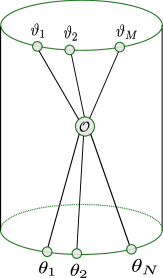
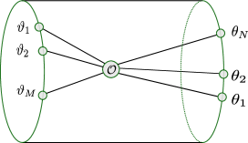
Figure 2: On the left: graphical representation of a finite volume form factor with incoming state $|\theta_{1},\dots,\theta_{N}\rangle$ and outgoing state $|\vartheta_{1},\dots,\vartheta_{M}\rangle$. Particles’ trajectories are schematically drawn as solid lines and the operator ${\cal O}$ is represented as a circle. On the right: the same form factor is represented after double Wick rotation in the thermal channel, i.e. when the Euclidean time is finite and space is infinite.

Exchanging the role of Euclidean space and time leads to the picture on the right of Figure 2, where we have to calculate a normalized trace:

$$\frac{\mbox{Tr}(e^{-LH}\mathcal{O}_{N,M})}{\sqrt{\mbox{Tr}_{N}(e^{-LH})\mbox{Tr}_{M}(e^{-LH})}}$$ (3.22)

In this channel $\mathcal{O}_{N,M}$ is not a local operator as moving a particle with rapidity $v$ around it picks up the phase $\prod_{j}S(v-\theta_{j}-\frac{i\pi}{2})\prod_{k}S(\vartheta_{k}+i\frac{\pi}{2}-v)$. This is the reason why we cannot apply a finite volume regularization as the system cannot be made periodic: the past/future or the left/right asymptotics are different. Particularly, in case of diagonal form factors, there is no monodromy and we could impose a periodic boundary condition in a finite volume. Clearly the normalization in this case would be the excited state partition function: $Z_{N}=\mbox{Tr}_{N}(e^{-LH})$. A particle with rapidity $\theta$ act in this channel as a defect operator with transmission factor $T(v)=S(\frac{i\pi}{2}+\theta-v)$.

In evaluating the trace we insert two complete systems of states

$$\mbox{Tr}(e^{-LH}\mathcal{O}_{N,M})=\sum_{\nu,\mu}\langle\nu|O_{N,M}|\mu\rangle\langle\mu|\nu\rangle e^{-E_{\nu}L}$$ (3.23)

and keep only the vacuum and one-particle states for $\mu$ and $\nu$ with rapidities $u$ and $v$. Infinite volume states are normalized as $\langle u|v\rangle=2\pi\delta(u-v)$ and the matrix element of the defect operator ${\cal O}_{N,M}$ can be expressed in terms of the infinite volume form factor as

$$\langle v|O_{N,M}|u\rangle = F_{N+M+2}(v+i\pi-i\epsilon,\{\vartheta+\frac{i\pi}{2}\},u,\{\theta-\frac{i\pi}{2}\})+$$

$$2\pi\delta(v-u)\prod_{j}S(\frac{i\pi}{2}+\vartheta_{j}-u)F_{N+M}(\{\vartheta+\frac{i\pi}{2}\},\{\theta-\frac{i\pi}{2}\})$$

Therefore, we are faced with the square of the $\delta$-function. Using our experience from evaluating the finite temperature 2-point function [24] we regulate the $\delta$-function as

$$2\pi\delta(u-v)=\frac{i}{u-v+i\epsilon}-\frac{i}{u-v-i\epsilon}$$ (3.25)

For the 2-point function this regularization was equivalent to finite volume regularizations [24]. Then, we shift the $v$ contour from the real line to above $i\epsilon$. Taking the $\epsilon\to 0$ limit, in the shifted integral no contribution will survive thus we merely pick up the residue term at $v=u+i\epsilon$. For the excited state partition function this results in

$$\mbox{Tr}_{N}(e^{-LH})=1+\int\frac{du}{2\pi}\frac{1}{\epsilon}\prod_{j}S(\frac{i\pi}{2}+\theta_{j}-u)e^{-mL\cosh u}+O(\epsilon)$$ (3.26)

Note that there is no $O(1)$ term. This is consistent with the usual evaluation of the partition function: if we calculated the contribution via finite volume regularization we would get $mR\cosh u$ instead of $\frac{1}{\epsilon}$. By repeating the same steps for the numerator we can check that the singular $\frac{1}{\epsilon}$ terms cancel with the square rooted product of the excited state partition functions and we find that the $O(1)$ piece is:

$$\delta^{(F)}F_{N+M}(\{\vartheta+i\pi\},\{\theta\})=\int\frac{du}{2\pi}F_{N+M+2}^{r}(u+i\pi,\{\vartheta+\frac{i\pi}{2}\},u,\{\theta-\frac{i\pi}{2}\})e^{-mL\cosh u}$$ (3.27)

where the previously introduced regulated form factor appears. In Appendix C we show that taking an appropriate residue of this $F$-term, the $\mu$-term (3.19) can be obtained.

4 Numerical comparison

In this section we check our results numerically by using the TCSA method in the sinh-Gordon and scaling Lee-Yang models. The TCSA method was first implemented for the Lee-Yang model by Yurov and Zamolodchikov [34]. Recently there has been a renewed interest in implementing it for the relevant perturbations of the noncompact free boson, see e.g. [35], [36] and [37].

Both in the sinh-Gordon and scaling Lee-Yang models we compare the analytical and TCSA results for the finite size energy spectrum then extract the finite volume matrix elements. After having checked the polynomial corrections we check the $F$-term corrections in the sinh-Gordon model and the $\mu$- and $F$- term corrections in the scaling Lee-Yang model.

4.1 Sinh-Gordon theory

The sinh-Gordon theory can be defined as

$$S=\int dt\int_{0}^{L}dx\,\left\{\frac{g}{2}(\partial_{\mu}\varphi)^{2}-2\mu\cosh(b\varphi)\right\}$$ (4.1)

When quantizing the theory we need to choose a scheme, which separates the free part and the perturbation. The free part can be either the free massless or massive boson and then the perturbing operator should be normal ordered wrt. the chosen free theory.

4.1.1 Conformal scheme

In the conformal scheme the free part is simply the kinetic term and the field has the following mode expansion

$$\varphi(x,t)=\varphi_{0}+\frac{\pi_{0}}{gL}t+\frac{i}{\sqrt{4\pi g}}\sum_{n\neq 0}\frac{1}{n}(a_{n}e^{ik_{n}(x-t)}+\bar{a}_{n}e^{-ik_{n}(x+t)});\quad k_{n}=\frac{2\pi n}{L}$$ (4.2)

where the nonzero commutators for the oscillators are $[a_{n},a_{m}]=n\delta_{n+m}$ and $[\bar{a}_{n},\bar{a}_{m}]=n\delta_{n+m}$. The zero mode is the free motion on the line with $[\varphi_{0},\pi_{0}]=i$. The Hilbert space is the superposition of the quantum mechanical zero mode with a continuous spectrum and the Fock space of left- and right-moving particles:

$$\mathcal{H}=\{a_{-n_{1}}\dots a_{-n_{k}}\bar{a}_{-m_{1}}\dots\bar{a}_{-m_{j}}|0\rangle\otimes\Psi(\varphi_{0})\}$$ (4.3)

The free Hamiltonian is then

$$H_{0}=\frac{2\pi}{L}(L_{0}+\bar{L}_{0}-\frac{1}{12})+\frac{\pi_{0}^{2}}{2gL}\quad;\qquad L_{0}=\sum_{n>0}a_{-n}a_{n}$$ (4.4)

This theory has conformal invariance. When the perturbing operators $:e^{\pm b\varphi}:$ are normal ordered wrt. this theory, they are primary fields of dimension $h=\bar{h}=-b^{2}\left(8\pi g\right)^{-1}$. The mass-gap relation [38]

$$-\frac{\pi\mu\Gamma\left(1+\frac{b^{2}}{8\pi g}\right)}{\Gamma\left(-\frac{b^{2}}{8\pi g}\right)}=\left[\frac{m}{4\sqrt{\pi}}\Gamma\left(\frac{1-p}{2}\right)\Gamma\left(1+\frac{p}{2}\right)\right]^{\frac{2}{1-p}}=(m\kappa)^{\frac{2}{1-p}}$$ (4.5)

connects the perturbation parameter of the Lagrangian $\mu$ to the mass, $m$, of the sinh-Gordon scattering particle, while the scattering parameter $p$ is related to $b$ as $p=\frac{b^{2}}{8\pi g+b^{2}}$.

In order to use the TCSA method, a discrete spectrum needs to be truncated at a given energy cut such that the full Hamiltonian can be diagonalized on the truncated space. To ensure this we separate the zero mode into a mini-Hilbert space with Hamiltonian

$$H_{\textrm{mini}}=\frac{1}{4\pi g}\pi_{0}^{2}+\mu\biggl{(}\frac{L}{2\pi}\biggr{)}^{2+\frac{b^{2}}{4\pi g}}2\pi(e^{b\varphi_{0}}+e^{-b\varphi_{0}})$$

where the volume-dependent coefficient comes from the conformal mapping of the Hamiltonian between the cylinder and the plane

$$H=\frac{2\pi}{L}\left(L_{0}+\bar{L}_{0}-\frac{1}{12}+H_{\mathrm{mini}}+\mu\biggl{(}\frac{L}{2\pi}\biggr{)}^{2+\frac{b^{2}}{4\pi g}}2\pi\delta_{P}\left\{e^{b\varphi_{0}}(:e^{b\hat{\varphi}}:-1)+e^{-b\varphi_{0}}(:e^{-b\hat{\varphi}}:-1)\right\}\right)$$ (4.6)

Here $\delta_{P}$ projects to matrix elements which do not change the momentum $P=\frac{2\pi}{L}(L_{0}-\bar{L}_{0})$ and $\hat{\varphi}=\varphi(0,0)-\varphi_{0}$. Technically, we solve numerically the mini-Hilbert space problem first. This can be done either in the basis of plane waves in a box or using the eigenvectors of the harmonic oscillator. For small volumes even the Liouville reflection factor can be used to get an approximation of the spectrum [38, 39]. We found that using 100 unperturbed vectors we got a reliable spectrum up to 5 digits in the range we were interested in. We kept 6-8 vectors from this zero mode space and calculated the matrix elements of $e^{\pm b\varphi_{0}}$. By taking the tensor product with the Fock spaces and truncating in the energy with only the zero mode perturbation added we obtained a finite Hilbert space. We then diagonalized the full Hamiltonian and calculated the eigenvalues and eigenvectors. These provided the finite size spectrum and finite volume form factors.

4.1.2 Massive boson scheme

Alternatively, one can start by perturbing the free boson of mass $M$. The free massive boson on the cylinder can be considered as a perturbation of the massless one, i.e.

$$H_{0}^{\left(M\right)}=H_{0}+g\frac{M^{2}}{2}\intop_{0}^{L}:\varphi\left(x,0\right)^{2}:dx$$ (4.7)

This operator can be diagonalized by solving the zero mode harmonic oscillator and applying a Bogoliubov transformation to the finite momentum oscillators. Technical details are relegated to Appendix D. As a result the field operator (4.2) is expressed in terms of the new massive creation operators $d_{n}$ as

$$\varphi\left(x,0\right)=\varphi_{0}+\sum_{n\neq 0}\frac{1}{\sqrt{2L\omega_{n}g}}\left(d_{n}e^{ik_{n}x}+d_{n}^{\dagger}e^{-ik_{n}x}\right)\quad;\qquad\omega_{n}=\sqrt{M^{2}+k_{n}^{2}}$$ (4.8)

while the Hamiltonian (4.7) becomes

$$H_{0}^{\left(M\right)}=\sum_{m\in\mathbb{Z}}\omega_{m}d_{m}^{\dagger}d_{m}+\tilde{E}_{0}^{\prime}$$ (4.9)

These operators satisfy $[d_{m}^{\dagger},d_{n}]=\delta_{n,m}$ and the vacuum energy contribution $\tilde{E}_{0}^{\prime}$ appears due to the difference between the normal ordering with respect to the mode operators $a_{n}$ or $d_{n}$.

When considering the sinh-Gordon model as a perturbation of the massive boson (e.g. to make a Feynman graph expansion), one may first define the Hamiltonian in infinite volume

$$H^{\left(L\rightarrow\infty\right)} =H_{0}^{\left(M,L\rightarrow\infty\right)}+\frac{gM^{2}}{b^{2}}\intop_{-\infty}^{\infty}:\cosh\left(b\varphi\left(x\right)\right):_{M,\infty}dx-\frac{gM^{2}}{2}\intop_{-\infty}^{\infty}:\varphi^{2}\left(x\right):_{M,\infty}dx$$

$$H_{0}^{\left(M,L\rightarrow\infty\right)}=\intop_{-\infty}^{\infty}\sqrt{M^{2}+k^{2}}d_{k}^{\dagger}d_{k}dk$$ (4.10)

Here $::_{M,\infty}$ means normal ordering with respect to the modes $d_{k}$ in infinite volume. We first connect the bare parameter $M$ to the bare coupling $\mu$ in the conformal plus zero mode scheme. As a first step, $H^{\left(L\rightarrow\infty\right)}$ is connected to the Hamiltonian on the cylinder. This is achieved by requiring that the perturbation has the same behavior in the UV, i.e. the Hamiltonian density expressed in terms of bare fields takes the same form for all volumes:

$$H=H_{0}^{\left(M\right)}+\frac{gM^{2}}{b^{2}}\intop_{0}^{L}:\cosh\left(b\varphi\left(x\right)\right):_{M,\infty}dx-\frac{gM^{2}}{2}\intop_{0}^{L}:\varphi^{2}\left(x\right):_{M,\infty}dx+\tilde{E}_{0}$$ (4.11)

By introducing a UV momentum cutoff in Appendix D we show that

$$:e^{b\varphi\left(0,0\right)}:_{M,\infty}=e^{\frac{b^{2}}{2g}\rho\left(ML\right)}:e^{b\varphi\left(0,0\right)}:_{M,L}\quad;\qquad\rho\left(x\right)=\intop_{-\infty}^{\infty}\frac{du}{2\pi}\frac{1}{e^{x\cosh u}-1}$$ (4.12)

Note that, similarly to Landau-Ginsburg theories, and as opposed to the sine-Gordon theory, the coefficient diverges in the limit $L\rightarrow 0$. Now, we bring the zero mode exponentials out of normal ordering and obtain the relation

$$\mu=\frac{gM^{2+\frac{b^{2}}{4\pi g}}}{2b^{2}}\left(\frac{e^{\gamma_{E}}}{2}\right)^{\frac{b^{2}}{4\pi g}}$$ (4.13)

together with the vacuum energy contribution

$$\tilde{E}_{0}=-\frac{M}{4}+\intop_{0}^{1}du\left(\frac{u}{\tanh\left(\frac{MLu}{2}\right)}-\frac{1}{2\left(1+u\right)^{2}\tanh\left(\frac{ML}{2\sqrt{1-u^{2}}}\right)}\right)$$ (4.14)

Following the same line of thought, the normalization of vertex operators can be related in the massive and massless schemes as well, as:

$$\left\langle e^{a\varphi}\right\rangle \equiv\left(\frac{L}{2\pi}\right)^{\frac{a^{2}}{4\pi g}}\left\langle\mathbf{0}\left|:e^{a\varphi\left(z=1,\bar{z}=1\right)}:_{0}\right|\mathbf{0}\right\rangle=e^{-\frac{a^{2}\gamma_{E}}{4g\pi}}\left(\frac{2}{M}\right)^{\frac{a^{2}}{4g\pi}}\left\langle\mathbf{0}\left|:e^{a\varphi\left(0\right)}:_{M,\infty}\right|\mathbf{0}\right\rangle$$ (4.15)

where $\left|\mathbf{0}\right\rangle$ denotes the interacting ground state.

We applied Hamiltonian truncation in this scheme, too. The zero mode problem is again treated separately, similarly to [40] and [41]. Comparing the results obtained from the massive scheme to the results in the massless scheme provided a tool to estimate the numerical error of our approach. Results are presented in the next subsection.

4.1.3 Numerical checks

For the numerical checks, we fixed $g=1$, such that $b_{\text{self-dual}}=\sqrt{8\pi}$. The UV coupling was fixed to $\mu=0.2$. The mini Hilbert space was chosen to be diagonalized on the particle in a rigid box basis with $800$ states per parity sector. It was sufficient to keep only the $6$ states of lowest energy out of these [40, 41]. In the Fock subspace, a conformal cutoff at chiral levels up to $9$ (in the finite momentum sector, $9$ and $10$) was used. The dominant cutoff dependence of the results came from this chiral cutoff. This means that the actual computations involved matrices of up to about $12000$ dimensions. Since the overall momentum is conserved as well as there is a parity $\mathbb{Z}_{2}$ symmetry present, it suffices to search the lowest lying eigenpairs of the appropriate sub-Hamiltonians restricted to the different symmetry sectors. The above cutoff should be understood separately in each subsector.

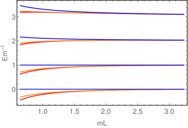
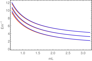
Figure 3: Theoretical low-lying energy spectrum of sinh-Gordon model at $b=1$. The vacuum energy density is subtracted. Left: states in the sector of overall momentum $0$ (from the bottom up: $\left|\mathrm{vac}\right\rangle$, $\left|0\right\rangle,$ $\left|00\right\rangle$ and $\left|000\right\rangle$). Right: states of overall momentum $1\cdot 2\pi L^{-1}$ (from the bottom up: $\left|1\right\rangle$, $\left|01\right\rangle$ and $\left|001\right\rangle$). Note that we label the states by the corresponding bosonic Bethe Ansatz quantization numbers. Bethe-Yang lines are drawn with blue curves. The leading Lüscher correction is depicted by orange curves. The exact TBA result is shown with red curves.

The strategy of the computations was to diagonalize the Hamiltonian (4.6) or (4.10) for a number of volumes, and then plot the volume dependence of the results. A typical spectrum can be seen on Figure 3.

Finite volume energies

In order to compare the TCSA energies to those obtained by solving the integral equation (2.6)-(2.8), it is important to keep in mind that the latter is renormalized fixing both the infinite volume energy and energy density to $0$. This scheme can be connected to the numerics obtained by TCSA by subtracting the (exactly known) vacuum energy density of the sinh-Gordon model

$$\mathcal{E}_{0}=\frac{m^{2}}{8\sin\pi p}\quad,\quad\quad p=\frac{b^{2}}{b^{2}+8\pi g}$$ (4.16)

We note that the TCSA numerics produce reliable results at $b=1$ for both the energy levels and the finite volume form factors. For stronger couplings, e.g. $b=2$, the truncation errors become more significant, see fig. 4. Experience suggests the general rule of thumb, using the massive oscillator basis (keeping the same excitation content of the basis) is equivalent to increasing the chiral cutoff of the massless TCSA basis by one. Therefore, for the present work, we mostly consider the case $b=1$.

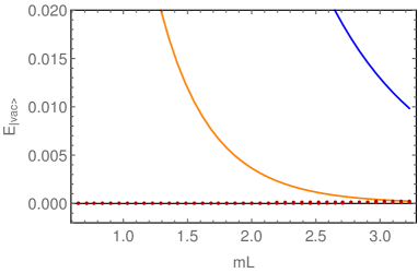
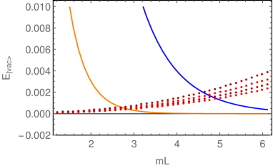
Figure 4: Volume dependence of the ground state energy: comparison of TCSA data with BY, Lüscher and TBA predictions for $b=1$ (left) and $b=2$ (right). On these plots, the TBA predictions are subtracted from each data set. TCSA measurement points are shown with red and brown dots, corresponding to different chiral cutoffs (from bottom up: $9,8,7$ and $6$). The difference between the BY lines and TBA (blue) and between BY+leading Lüscher and TBA (orange) are also indicated. For $b=1$, TCSA results agree with TBA data to a remarkable precision (the difference is negligible, as well as the cutoff dependence thereof). For $b=2$ truncation errors become more significant.

To make the results more transparent, we chose to depict the difference of the quantities of interest from some reference data. In Figs. 4-5, the results obtained by numerically solving the TBA system (2.6)-(2.8) are subtracted from each other data sets (in the case of the TCSA points, the energy density (4.16) is also taken into account). Note that we label the states by the corresponding Bethe Ansatz quantization numbers. The Bethe-Yang lines are calculated via (2.9)-(2.11), while the exponential corrections follow from (2.12)-(2.15).

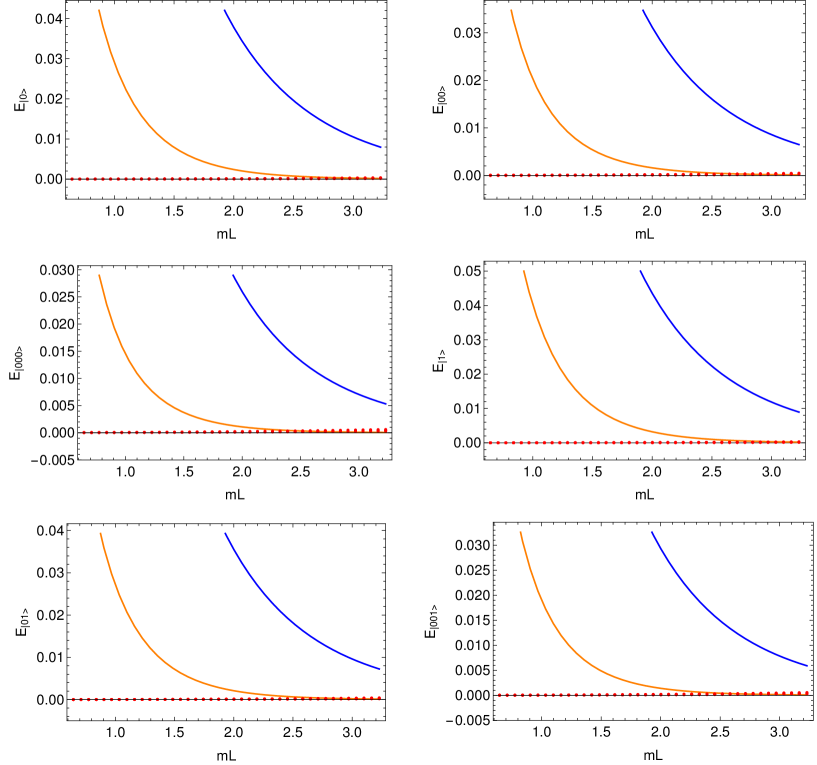
Figure 5: Volume dependence of the energy of some relevant low-lying states at $b=1$. Again, TBA data are subtracted from each data set. TCSA data is shown by red dots. The difference between the BY lines and TBA (blue) and between BY+leading Lüscher and TBA (orange) are also indicated. Once again, we see reassuring agreement between the TBA and TCSA data (the difference being close to $0$, as shown.)

From these plots it is clear that in the volume range 1-3 the numerical results can be trusted and that adding the leading exponential correction to the Bethe-Yang results considerably improved the precision. We expect similar behaviors for finite volume form factors.

Finite volume form factors

In order to check our results in subsection (3.3) we analyze the finite size form factors of the elementary field and the exponential operators $\mathcal{O}_{k}=:e^{kb\varphi}:$. For both cases the infinite volume form factors have the form (3.7) with

$$P_{n}^{\mathcal{O}_{k}}=\det_{i,j}|[i-j+k]\sigma_{2i-j}|\quad;\qquad[k]=\frac{\sin k\pi p}{\sin\pi p}$$ (4.17)

where we used the basis of symmetric polynomials defined by

$$\prod_{i=1}^{n}(z+x_{i})=\sum_{k=0}^{n}\sigma_{k}z^{n-k}$$ (4.18)

The normalization for the elementary field is given by $H_{2n+1}^{\varphi}=\sqrt{\frac{Z\left(b\right)}{2}}\left(\frac{4\sin\pi p}{f(i\pi)}\right)^{n}$, where $Z\left(b\right)$ is the wavefunction renormalization constant [42]

$$Z\left(b\right)=\frac{8\pi^{2}p^{2}g}{b^{2}\sin\left(\pi p\right)f\left(i\pi\right)}$$ (4.19)

In the plots regarding the finite volume form factors (Figures 6 and 7), the numerical TCSA data is subtracted. Then the “error” of the polynomial (3.11) approximation (more precisely, its difference from TCSA numerics), as calculated from (3.7) and (3.11), is shown by dashed lines. Solid curves depict the results of the present paper ((3.21), (3.27)).

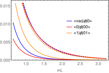
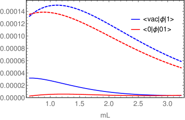
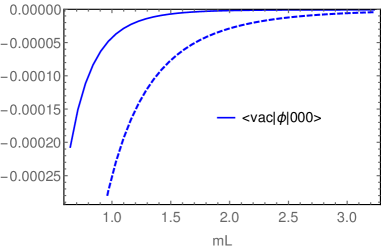
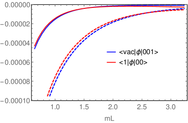
Figure 6: Theoretical predictions for various finite volume form factors of the field $\phi$, as compared to numerical TCSA data (the latter is subtracted from each data set) at $b=1$. Polynomial (Pozsgay-Takács) results are depicted by dashed curves, while the results containing the first exponential corrections, conjectured by the present article, are shown by continuous curves.

The normalization for the exponentials is given by $H_{n}^{k}=\left\langle\mathcal{O}_{k}\right\rangle\left(\frac{4\sin\pi p}{f(i\pi)}\right)^{\frac{n}{2}}$, where $\left\langle\mathcal{O}_{k}\right\rangle$ is given by the Lukyanov-Zamolodchikov formula [43]:

$$\left\langle\mathcal{O}_{k}\right\rangle =m^{-\frac{k^{2}b^{2}}{4\pi g}}\left[\frac{\Gamma\left(\frac{1-p}{2}\right)\Gamma\left(1+\frac{p}{2}\right)}{4\sqrt{\pi}}\right]^{-\frac{k^{2}b^{2}}{4\pi g}}$$ (4.20)

$$\exp\intop_{0}^{\infty}\frac{dt}{t}\left[-\frac{\sinh^{2}\left(\frac{kb^{2}t}{4\pi g}\right)}{2\sinh\left(\frac{b^{2}t}{8\pi g}\right)\sinh t\cosh\left[\left(1+\frac{b^{2}}{8\pi g}\right)t\right]}+\frac{k^{2}b^{2}}{4\pi g}e^{-2t}\right]$$

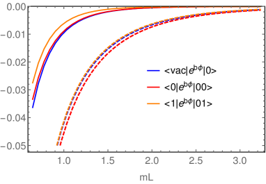
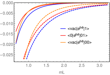
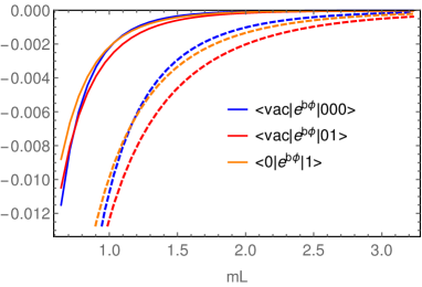
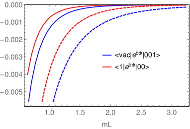
Figure 7: Theoretical predictions for various finite volume form factors of the primary operator $e^{b\varphi}$, as compared to numerical TCSA data (the latter is subtracted from each data set) at $b=1$. Polynomial (Pozsgay-Takács) results are depicted by dashed curves, while the results containing the first exponential corrections, conjectured by the present article, are shown by continuous curves.

On figure 8 we also present some additional checks for the operators $e^{1.5b\varphi}$ and $e^{2b\varphi}$.

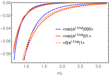
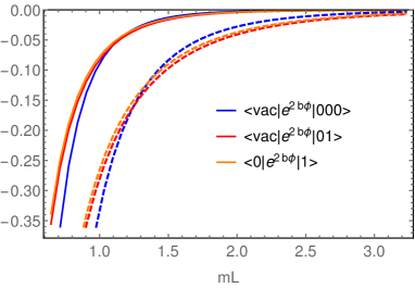
Figure 8: Additional checks to some form factors of $e^{1.5b\varphi}$ and $e^{2b\varphi}$. Polynomial (Pozsgay-Takács) results are depicted by dashed curves, while the results containing the first exponential corrections, conjectured by the present article, are shown by continuous curves. Again, the TCSA results are subtracted from each data set.

As shown on all of the plots including the theoretically predicted leading exponential correction improved the data the same way as the similar corrections improved the energy spectrum. This is a very strong support for our conjectured $F$-term formulae. Let us see the analogous results for the scaling Lee-Yang theory.

4.2 Scaling Lee-Yang theory

The scaling Lee-Yang theory is the only relevant perturbation of the conformal Lee-Yang model:

$$S=S_{LY}+\lambda\int d^{2}z\,\Phi(z,\bar{z})$$ (4.21)

The conformal Lee-Yang model is the simplest non-unitary minimal model with central charge $c=-\frac{22}{5}$. There are two highest weight representations: one corresponds to the identity operator and the other one to the perturbing field $\Phi(z,\bar{z})$ with dimension $(-\frac{1}{5},-\frac{1}{5})$. The Hamiltonian can be written on the plane as

$$H=\frac{2\pi}{L}(L_{0}+\bar{L}_{0}-\frac{c}{12})+\lambda\biggl{(}\frac{L}{2\pi}\biggr{)}^{2+2/5}2\pi\delta_{P}\Phi(0,0)$$ (4.22)

The parameter $\lambda$ is related to the mass of the scattering particles as

$$m=\frac{2^{\frac{19}{5}}\sqrt{\pi}(\Gamma(\frac{3}{5})\Gamma(\frac{4}{5})\lambda)^{\frac{5}{12}}}{5^{\frac{5}{16}}\Gamma(\frac{2}{3})\Gamma(\frac{5}{6})}$$ (4.23)

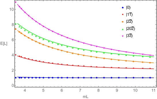
Figure 9: Low lying finite size energy spectrum of the scaling Lee-Yang model obtained from TCSA with the ground state energy density subtracted. Continuous lines are the results of the Bethe-Yang equations with the various quantization numbers, while discrete data originates from TCSA.

The conformal Hilbert space is generated by acting with the negative Virasoro modes on the highest weight states. On this space $L_{0}$ and $\bar{L}_{0}$ act diagonally and the matrix elements of $\Phi(0,0)$ can be calculated exactly. Similarly to the analysis of the sinh-Gordon model, we truncate the Hilbert space and diagonalize $H$ on this space to obtain the energy spectrum and the form factors of the perturbing operator. The ground state energy density in the TCSA and the TBA formulation are different. To relate the TCSA to the TBA results the ground state energy density

$$\epsilon=-\frac{m^{2}}{4\sqrt{3}}\text{ }$$ (4.24)

has to be subtracted. The finite size spectrum obtained by the TCSA method after the subtraction looks like in Figure 9.

In order to visualize the various finite size corrections we subtract the numerical TCSA data from the theoretical curves as shown on Figure 10. In the domain investigated we compared the TCSA data to the exact TBA result and found that it’s precision was $10^{-5}$. Thus there is no visual difference in subtracting TCSA compared to the exact results. For the form factors we do not know the exact results, therefore we can only subtract the TCSA data and this is the reason why we followed this approach here. The Bethe-Yang correction (2.10) contains the polynomial volume corrections. The $F_{1}$ term is the leading $F$-term correction (2.15), while $\mu_{1}$ is the leading $\mu$-term correction (2.28). The $\mu$ correction sums up all the $\mu$-terms by solving (2.21) for the constituents. Then we combine these $\mu$-terms corrections with the leading $F$-term corrections.

Figure 10: Exponential finite size energy correction for the state labeled by the quantum numbers $\{2,0,-2\}$. “$F_{1}$” is the F-term correction, while “$\mu_{1}$” is the leading $\mu$-term correction. “$\mu$” contains all the $\mu$-term corrections summed up, while “$\mu+F_{1}$” adds the $F$-term correction to this.

Neither the $F$-term nor the $\mu$-term correction gives a good approximation for volumes $7-13$, however their sum is very close to result of the numerics. The best approximation arises from combining the summed up $\mu$-term correction with the leading $F$-term correction.

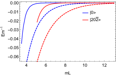
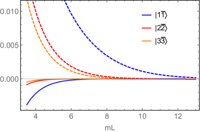
Figure 11: Demonstration of the polynomial and exponential volume corrections for the energy. Dashed lines are the difference between the Bethe-Yang energies and TCSA data and solid lines are the difference of the best $\mu+F$ approximation and the TCSA data. The energy cut is $16$.

The best results are demonstrated on figure (11). These suggest that we understand the finite size correction of the energy levels very well, thus we now turn to the investigation of finite volume form factors.

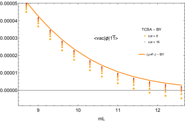
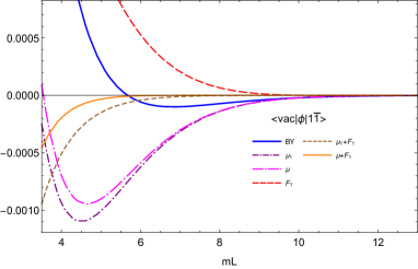
Figure 12: Left: Cut dependence of the TCSA data. The difference of the TCSA and the BY data at different cuts is marked by dots with various colours and the difference between the $\mu+F_{1}$ and BY data is represented with a solid line. Right: Volume corrections of the form factor $\langle\mathrm{vac}|\Phi|\{1,-1\}\rangle$. Every line shows the absolute value of the difference between the given theoretical curve and the TCSA data.

The infinite volume form factors of the perturbing operators are given by (3.7) with

$$\langle\Phi\rangle=\frac{3^{\frac{9}{10}}\Gamma(\frac{1}{3})^{\frac{36}{5}}}{(2\pi)^{\frac{14}{5}}5^{\frac{1}{4}}\Gamma(\frac{1}{5})\Gamma(\frac{2}{5})}\quad;\qquad H_{n}=\left(\frac{\Gamma}{\sqrt{f(i\pi)}}\right)^{n}$$ (4.25)

and with $P_{1}=1$, $P_{2}=\sigma_{1}$ and for $n>2$

$$P_{n}(x_{1},\dots,x_{n})=\sigma_{1}\sigma_{n-1}\det_{ij}\left|\sigma_{3i-2j+1}\right|$$ (4.26)

where we used the basis of symmetric polynomials.

Similarly to the energy spectrum we subtract the TCSA data from the various theoretical curves. Such a result is displayed on Figure 12. The BY curves are the result of (3.11), the leading $\mu$-term correction denoted as $\mu_{1}$ is given by (3.20) and the leading $F$-term correction, $F_{1},$ by (3.27). Plugging the solution of (2.21) into the asymptotic formula (3.13) the form factor $\mu$-terms can be summed up. This correction is denoted by $\mu$. Finally, adding the leading $F$-term to the $\mu$-terms leads to the best approximations.

On figure (13) we demonstrate the BY and the best $\mu+F_{1}$ corrections for various states.

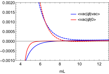
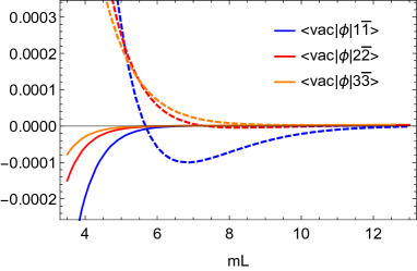
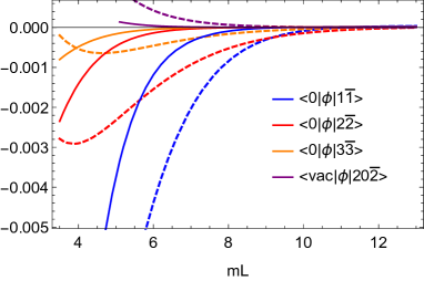
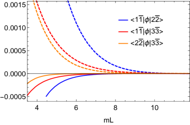
Figure 13: Representative figures for the polynomial and exponential corrections. Dashed lines are the absolute values of the difference between the BY and TCSA data, while solid lines are the same for the best available exponential corrections. For the $\langle\mathrm{vac}|\Phi|\mathrm{vac}\rangle$ diagonal matrix element we show the F-term only. For $\langle\mathrm{vac}|\Phi|\{0\}\rangle,\langle\mathrm{vac}|\Phi|\{n,-n\}\rangle$ the best available correction is “$\mu+F_{1}$”, while for $\langle\{0\}|\Phi|\{n,-n\}\rangle,\langle\mathrm{vac}|\Phi|\{2,0,-2\}\rangle,\langle\{m,-m\}|\Phi|\{n,-n\}\rangle;\;n,m=1,2,3$: best available correction is “$\mu_{1}+F_{1}$”

In summary, the data presented gives a strong evidence for the correctness of our exponential finite size corrections.

5 Conclusion

In this paper we presented the leading exponentially small volume corrections for non-diagonal form factors in diagonally scattering theories. In theories with bound states the leading correction is the $\mu$-term, which we derived using the asymptotic finite volume form factor and the assumption that particles are composed of their constituents. The $F$-term is universal in the sense that it is present in theories both with and without bound states, providing the next and leading exponential correction, respectively. We derived the $F$-term formally and tested the results in various ways.

We showed that by taking appropriate residues of the integral for the rapidities of the virtual particles we can completely recover the $\mu$-term correction. We checked that taking the diagonal limit of the form factors, by sending one rapidity to infinity based on [17] reproduced the diagonal result of [22]. By developing numerical methods to “measure” the finite volume form factors we tested the finite size corrections in the sinh-Gordon and Lee-Yang models, where we found convincing confirmation of our formulae.

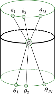
Figure 14: Graphical representation of the form factor $F$-term Lüscher correction. A virtual particle pair appears from the vacuum and after travelling around the world is absorbed by the operator.

Figure 14 visualizes the physical picture behind the $F$-term: First a virtual particle-anti-particle pair appears from the finite volume vacuum, then one of them travels around the world and finally both are absorbed by the operator. Since the infinite volume form factor with a particle-anti-particle pair is singular we had to regulate the appearing amplitude. Our complicated derivation and checks resulted in the proper definition of this regulated form factor. We found that we had to subtract the kinematical singularity of the form factor in a symmetric way (B.14). This regulated form factor has very nice properties. Its phase is the same as the original form factor’s for which we are calculating the correction. Its singularities on the upper and lower half planes are related to each other, in such a way that the $\mu$-term corrections are correctly reproduced when the residues are taken . In the simplest non-trivial (vacuum-one-particle) form factor it is real and reproduces our previous results [24], which we derived using a finite volume analogue of the LSZ reduction formula of the two-point function.

We approached the problem of calculating the partition function and evaluating the asymptotic form factor for bound states through systematic large volume expansions. Clearly this method can be used at higher orders and the resulting finite size form factors give the building blocks of the finite size or finite temperature correlation functions. These can be used in statistical physical or solid state systems as well as in the AdS/CFT duality. Although the expansion can be useful for practical applications, for obtaining exact results the series has to be summed up. In this respect the integral equation derived recently for diagonal form factors in the sinh-Gordon theory can be useful [44].

Acknowledgments

We would like to thank Aron Bodor for the collaboration at an early stage of this work. Furthermore, Janos Balog, Arpad Hegedus, Fedor Smirnov and Gabor Takacs for the useful discussions. M.L. thanks to Robert Konik and Giuseppe Mussardo for the useful discussions regarding the TCSA method employed (see also footnote 5). This research was supported by the NKFIH research Grant K116505, the NKFIH Summer Student Internship Program and the Lendulet Program of the Hungarian Academy of Sciences.

Appendix A Derivation of the form factors’ $\mu$-term correction

In this Appendix we calculate the $\mu$-term correction for form factors in the scaling Lee-Yang model. We start with the order $\left(0\right)$ form factor

$$\langle 0|\mathcal{O}|\{\theta_{\pm}\}\rangle_{L}=\frac{F_{2N}(\theta_{1+},\theta_{1-},\ldots\theta_{N+},\theta_{N-})}{\sqrt{\prod\limits_{k}S(\theta_{k+,k-})\rho_{2N}(\{\theta_{\pm}\})\prod\limits_{i<j,s,k}S(\theta_{is,jk})}}$$ (A.1)

evaluated at $\theta_{j\pm}=\bar{\theta}_{j\pm}^{(\mu)}=\bar{\theta}_{j}^{(\mu)}\pm i(u+\delta\bar{u}_{j})$. Our aim is to expand this expression at leading order in $\delta\bar{u}_{j}$. We first multiply both the numerator and the denominator by $\left(\prod_{k}\frac{2\delta\bar{u}_{k}}{\Gamma}\right)$ in order to ensure that the expansion of the numerator starts with the form factor $F_{N}(\{\bar{\theta}^{(\mu)}\})$:

$$\prod_{k}\left(\frac{2\delta\bar{u}_{k}}{\Gamma}\right)F_{2N}(\{\bar{\theta}_{\pm}^{(\mu)}\})=F_{N}(\{\bar{\theta}^{(\mu)}\})+\sum_{k}\left(\frac{2\delta\bar{u}_{k}}{\Gamma}\right)F_{N,k}^{b}(\{\bar{\theta}^{(0)}\})+\dots$$ (A.2)

In evaluating the denominator we first combine the rows and columns of $\rho_{2N}$ to obtain the derivatives of $Q$ and $\bar{Q}$ with respect to $\partial$ and $\bar{\partial}$ as:

$$\rho_{2N}(\{\theta_{\pm}\}) =\det\left\{\frac{\partial\left(Q_{1+},Q_{1-},\ldots,Q_{N+},Q_{N-}\right)}{\partial\left(\theta_{1+},\theta_{1-},\ldots,\theta_{N+},\theta_{N-}\right)}\right\}=\frac{1}{4^{N}}\begin{vmatrix}\left[\bar{\partial}\bar{Q}\right]&\left[\bar{\partial}Q\right]\\ \left[\partial\bar{Q}\right]&\left[\partial Q\right]\end{vmatrix}$$

$$=\frac{1}{4^{N}}\det\left[\bar{\partial}\bar{Q}\right]\det\left\{\left[\partial Q\right]-\left[\partial\bar{Q}\right]\left[\bar{\partial}\bar{Q}\right]^{-1}\left[\bar{\partial}Q\right]\right\}$$ (A.3)

where $\left[\bar{\partial}\bar{Q}\right]_{ij}=\left[\bar{\partial}\bar{Q}\right]_{ji}=\bar{\partial}_{i}\bar{Q}_{j}^{(0)}(\{\theta_{\pm}\})$ with $\bar{\partial}_{i}=\partial_{i+}-\partial_{i-}$. Similarly $\left[\bar{\partial}Q\right]_{ij}=\left[\partial\bar{Q}\right]_{ji}=\bar{\partial}_{i}Q_{j}^{(0)}(\{\theta_{\pm}\})$ and $\left[\partial Q\right]_{ij}=\left[\partial Q\right]_{ji}=\partial_{i}Q_{j}^{(0)}(\{\theta_{\pm}\})$. Up to the next-to-leading order we can use that

$$\left(\frac{2\delta\bar{u}_{k}}{\Gamma}\right)^{2}S(\theta_{k+,k-})=\phi(2i(u+\delta\bar{u}_{k}))^{-1}+O((\delta\bar{u})^{3})=2\delta\bar{u}_{k}+\left(\frac{2\delta\bar{u}_{k}}{\Gamma}\right)^{2}S_{0}+O((\delta\bar{u})^{3})$$ (A.4)

thus there are poles of type $\delta\bar{u}_{k}^{-1}$ in the diagonal elements of $[\bar{\partial}\bar{Q}]$ originating from

$$\bar{\partial}_{j}\bar{Q}_{j}^{(0)}(\{\theta_{\pm}\})=4\phi(2i(u+\delta\bar{u}_{j}))+\partial_{j}Q_{j}^{(0)}(\{\theta_{\pm}\})$$ (A.5)

Expanding up to next-to-leading order gives

$$\left(\prod_{k}\frac{1}{4\phi(2i(u+\delta\bar{u}_{k}))}\right)\det\left\{\text{diag}[\{4\phi(2i(u+\delta\bar{u}_{k}))\}]+[\partial Q]\right\}\det\left\{\left[\partial Q\right]-\left[\partial\bar{Q}\right]\left[\bar{\partial}\bar{Q}\right]^{-1}\left[\bar{\partial}Q\right]\right\} =$$

$$\left(1+\sum_{k}\frac{1}{2}\partial_{k}Q_{k}^{(0)}(\{\theta\})\delta\bar{u}_{k}\right)\det\left\{\partial_{i}Q_{j}^{\left(0\right)}(\{\theta_{\pm}\})-\sum_{k}\frac{1}{2}\left[\partial\bar{Q}\right]_{ik}\left[\bar{\partial}Q\right]_{kj}\delta\bar{u}_{k}\right\}$$ (A.6)

where we used that at leading order $\left[\bar{\partial}\bar{Q}\right]^{-1}=\mathrm{diag}\left(\frac{\delta\bar{u}_{1}}{2},\ldots,\frac{\delta\bar{u}_{n}}{2}\right)$. It is natural to introduce the density of states corresponding to the quantization of order $(\mu$): $\rho_{N}^{\left(\mu\right)}(\{\theta\})$ as in (3.16). Evaluating now expression (A.6) at the solutions one can show that

$$\prod_{k}\left(\frac{2\delta\bar{u}_{k}}{\Gamma}\right)^{2}S(2i(u+\delta\bar{u}_{k}))\rho_{2N}(\{\bar{\theta}_{\pm}^{(0)}\})=\rho_{N}^{\left(\mu\right)}(\{\bar{\theta}^{(\mu)}\})\left(1+\sum_{k}\partial_{k}Q_{k}^{(0)}(\{\bar{\theta}^{(0)}\})\delta\bar{u}_{k}\right)$$ (A.7)

where we also used that

$$\det\left[\partial Q\right]\left\{1-\frac{1}{2}\sum_{k}\partial_{k}Q_{k}^{\left(0\right)}(\{\theta\})\delta\bar{u}_{k}\right\}=\det\left\{\left[\partial Q\right]_{ij}-\frac{1}{2}\sum_{k}\left[\partial Q\right]_{ik}\left[\partial Q\right]_{kj}\delta\bar{u}_{k}\right\}$$ (A.8)

Finally, we expand the product of scattering matrices as

$$S(\theta_{i+,j+})S(\theta_{i+,j-})S(\theta_{i-,j+})S(\theta_{i-,j-})=S(\theta_{i,j})\left(1+\bar{\partial}_{i}Q_{j}^{(0)}(\{\theta_{\pm}\})\delta u_{i}(\{\theta\})-\partial_{i}\bar{Q}_{j}^{\left(0\right)}(\{\theta_{\pm}\})\delta u_{j}(\{\theta\})\right)$$ (A.9)

Collecting all factors the $\mu$-term of the finite volume form factor can be parametrized as

$$\langle 0|\mathcal{O}|\{n\}\rangle_{L}=\frac{F_{N}(\{\bar{\theta}^{(\mu)}\})+\delta^{(\mu)}F_{N}(\{\bar{\theta}^{(\mu)}\})}{\sqrt{\prod\limits_{k<j}S(\bar{\theta}_{k,j}^{(\mu)})\rho_{N}^{(\mu)}(\{\bar{\theta}^{(\mu)}\})}}$$ (A.10)

where the $\mu$-term correction takes the form

$$\delta^{(\mu)}F_{N}(\{\bar{\theta}^{(\mu)}\}) =\sum_{k}\left\{\frac{2}{\Gamma}F_{N,k}^{b}(\{\bar{\theta}^{(0)}\})-\frac{1}{2}\partial_{k}Q_{k}^{(0)}(\{\bar{\theta}^{(0)}\})F_{N}(\{\bar{\theta}^{(0)}\})\right\}\delta\bar{u}_{k}$$

$$+\frac{1}{2}\sum_{k}\sum_{j<k}\left[\phi_{-}(\bar{\theta}_{j,k}^{(0)})\left(\delta\bar{u}_{j}+\delta\bar{u}_{k}\right)\right]F_{N}(\{\bar{\theta}^{(0)}\})$$ (A.11)

where we introduced $\phi_{-}(\theta)=\phi(\theta+2iu)-\phi(\theta-2iu)$.

Appendix B Formal derivation of the form factors’ $F$-term correction

In this Appendix we give a formal derivation of the leading exponential correction of the non-diagonal form factor. We work in a theory without bound states and focus on the F-term correction only. As we explained in the main text we have to evaluate the following expression

$$\frac{\mbox{Tr}(e^{-LH}\mathcal{O}_{N,M})}{\sqrt{\mbox{Tr}_{N}(e^{-LH})\mbox{Tr}_{M}(e^{-LH})}}$$ (B.1)

where the normalization is related to the excited state partition function

$$Z_{N}=\mbox{Tr}_{N}(e^{-LH})$$ (B.2)

which can be represented graphically as shown on Figure 15.

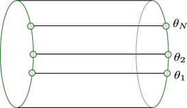
Figure 15: Graphical representation of the excited state partition function. A physical particle with rapidity $\theta_{j}$ serves as a defect operator with transmission factor $T(u)=S(\frac{i\pi}{2}+\theta_{j}-u)$.

In the general non-diagonal case, i.e. in formula (B.1) on the left half space we have the defect operator of the outgoing state and on the right half that of the incoming excited state. These half spaces are taken into account by the square roots in the normalization. This normalization factor is also understood as the removal of the operator in the trace, with keeping the incoming and outgoing particle lines.

In the analysis of thermal two-point function we showed for small particle numbers that infinite and finite volume normalizations can be equivalent if the $\delta$-function is regularized properly [24]. By following the same steps we introduce two complete systems of states to evaluate the trace:

$$\mbox{Tr}(e^{-LH}\mathcal{O}_{N,M})=\sum_{\nu,\mu}\langle\nu|O_{N,M}|\mu\rangle\langle\mu|\nu\rangle e^{-E_{\nu}L}$$ (B.3)

In the following we evaluate the leading 1-particle contribution. For the numerator we have

$$\mbox{Tr}(e^{-LH}O_{N,M})=F_{N+M}+\int\frac{du}{2\pi}\int\frac{dv}{2\pi}\langle v|O_{N,M}|u\rangle\langle u|v\rangle e^{-mL\cosh v}$$ (B.4)

while for the normalization factor we obtain

$$\mbox{Tr}_{N}(e^{-LH})=1+\int\frac{du}{2\pi}\int\frac{dv}{2\pi}\langle u|v\rangle\prod_{j}S(\frac{i\pi}{2}+\theta_{j}-v)\langle v|u\rangle e^{-mL\cosh v}$$ (B.5)

Since infinite volume states are normalized to Dirac delta functions $\langle u|v\rangle=2\pi\delta(u-v)$ we have to calculate the square of the $\delta$-function. This is an ambiguous quantity, but based on experience from the evaluation of the 2-point function we regulate the $\delta$-function as

$$2\pi\delta(u-v)=\frac{i}{u-v+i\epsilon}-\frac{i}{u-v-i\epsilon}$$ (B.6)

Then we shift the $v$ contour from the real line above $i\epsilon$. On the shifted integral the $\epsilon\to 0$ limit can be taken, such that due to the previous $\delta$-function no contribution will survive. Thus we only need the residue term at $v=u+i\epsilon$. Calculating the residue for the partition function we obtain:

$$\mbox{Tr}_{N}(e^{-LH})=1+\int\frac{du}{2\pi}\frac{1}{\epsilon}\prod_{j}S(\frac{i\pi}{2}+\theta_{j}-u)e^{-mL\cosh u}+O(\epsilon)$$ (B.7)

in which there is no $O(1)$ term. This is consistent with the usual evaluation of the partition function based on finite volume regularization where $mR\cosh u$ appears, instead of $\frac{1}{\epsilon}$ .

Let us focus on the form factor contribution. The matrix element $\langle v|O_{n,m}|u\rangle$ can be represented graphically as on Figure 16.

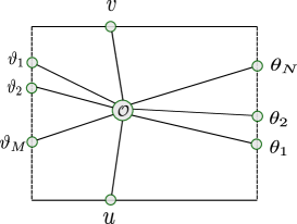
Figure 16: Graphical representation of the matrix element $\langle v|O_{n,m}|u\rangle$, which is the matrix element of the non-local operator ${\cal O}_{n,m}$.

Using the crossing properties of the form factors $\langle v|O_{N,M}|u\rangle$ can be written as

$$\langle v|O_{N,M}|u\rangle = F_{N+M+2}(v+i\pi-i\epsilon,\{\vartheta+\frac{i\pi}{2}\},u,\{\theta-\frac{i\pi}{2}\})+$$

$$2\pi\delta(v-u)\prod_{j}S(\frac{i\pi}{2}+\vartheta_{j}-u)F_{N+M}(\{\vartheta+\frac{i\pi}{2}\},\{\theta-\frac{i\pi}{2}\})$$

Alternatively, using the permutation property of the infinite volume form factors we can write

$$\langle v|O_{N,M}|u\rangle = \prod_{j}S(\frac{i\pi}{2}+\vartheta_{j}-u)F_{N+M+2}(v+i\pi-i\epsilon,u,\{\vartheta+\frac{i\pi}{2}\},\{\theta-\frac{i\pi}{2}\})+$$ (B.9)

$$2\pi\delta(v-u)\prod_{j}S(\frac{i\pi}{2}+\vartheta_{j}-u)F_{N+M}(\{\vartheta+\frac{i\pi}{2}\},\{\theta-\frac{i\pi}{2}\})$$

Separating the singular part of the form factor as

$$F_{N+M+2}(v+i\pi,u,\{\vartheta+\frac{i\pi}{2}\},\{\theta-\frac{i\pi}{2}\}) =\frac{i}{v-u}\biggl{(}1-\frac{\prod_{k}S(\frac{i\pi}{2}+\theta_{k}-u)}{\prod_{j}S(\frac{i\pi}{2}+\vartheta_{j}-u)}\biggr{)}F_{N+M}(\{\vartheta+\frac{i\pi}{2}\},\{\theta-\frac{i\pi}{2}\})$$

$$+F_{N+M+2}^{c}(v+i\pi,u,\{\vartheta+\frac{i\pi}{2}\},\{\theta-\frac{i\pi}{2}\})$$ (B.10)

and introducing the connected part of the form factor, such that combining this with the $\delta$-term we obtain:

$$\langle v|O_{N,M}|u\rangle = \prod_{j}S(\frac{i\pi}{2}+\vartheta_{j}-u)F_{N+M+2}^{c}(v+i\pi,u,\{\vartheta+\frac{i\pi}{2}\},\{\theta-\frac{i\pi}{2}\})+$$

$$\left(\frac{i\prod_{j}S(\frac{i\pi}{2}+\vartheta_{j}-u)}{v-u+i\epsilon}-\frac{i\prod_{k}S(\frac{i\pi}{2}+\theta_{k}-u)}{v-u-i\epsilon}\right)F_{N+M}(\{\vartheta+\frac{i\pi}{2}\},\{\theta-\frac{i\pi}{2}\})$$

Plugging this expression back to eq. (B.4) and evaluating the $v$ integral the same way we did for the partition functions we obtain the singular term

$$\frac{F_{N+M}(\{\vartheta+\frac{i\pi}{2}\},\{\theta-\frac{i\pi}{2}\})}{2\epsilon}\int\frac{du}{2\pi}\left\{\prod_{j}S(\frac{i\pi}{2}+\vartheta_{j}-u)+\prod_{k}S(\frac{i\pi}{2}+\theta_{k}-u)\right\}e^{-mL\cosh u}$$ (B.12)

This only cancels the singular term coming from the $\sqrt{Z_{N}Z_{M}}$ normalizations. The O(1) term gives the finite size correction

$$\int\frac{du}{2\pi}\left\{\prod_{j}S(\frac{i\pi}{2}+\vartheta_{j}-u)F_{N+M+2}^{c}(u+i\pi,u,\{\vartheta+\frac{i\pi}{2}\},\{\theta-\frac{i\pi}{2}\})-\hskip 113.81102pt\right.$$ (B.13)

$$\left.\frac{F_{N+M}(\{\vartheta+\frac{i\pi}{2}\},\{\theta-\frac{i\pi}{2}\})}{2}imL\sinh u\left(\prod_{j}S(\frac{i\pi}{2}+\vartheta_{j}-u)-\prod_{k}S(\frac{i\pi}{2}+\theta_{k}-u)\right)\right\}e^{-mL\cosh u}$$

which after integration by parts gives the regulated expression

$$F_{N+M+2}^{r}(u+i\pi,\{\vartheta+\frac{i\pi}{2}\},u,\{\theta-\frac{i\pi}{2}\})=\lim_{\epsilon\to 0}\biggl{\{}F_{N+M+2}(u+i\pi+\frac{\epsilon}{2},\{\vartheta+\frac{i\pi}{2}\},u-\frac{\epsilon}{2},\{\theta-\frac{i\pi}{2}\})\hskip 56.9055pt$$

$$-\frac{i}{\epsilon}\bigl{(}\prod_{j}S(\vartheta_{j}+\frac{i\pi}{2}-u)-\prod_{j}S(\theta_{k}+\frac{i\pi}{2}-u)\bigr{)}F_{N+M}(\{\vartheta+\frac{i\pi}{2}\},\{\theta-\frac{i\pi}{2}\})\biggr{\}}\hskip 56.9055pt$$ (B.14)

equivalent to(3.27).

Appendix C Relation between $\mu$- and $F$-terms

In this Appendix we show that, similarly to the Bethe-Yang equations and energy formulas, the $\mu$-term form factor corrections can be obtained by taking appropriate residues of the $F$-terms corrections. Due to the additive structure of the correction (3.20) we analyze the form factor only containing incoming particles. We start with the $F$-term formula

$$\langle 0|\mathcal{O}|\{n_{j}\}\rangle_{L} =\frac{F_{N}(\{\bar{\theta}^{(1)}\})+\delta^{(F)}F_{N}(\{\bar{\theta}^{\left(1\right)}\})}{\sqrt{\prod_{i<j}S(\bar{\theta}_{i,j}^{(1)})\rho_{N}^{(1)}(\{\bar{\theta}^{(1)}\})}}+\dots$$ (C.1)

where the $F$-term correction contains the regulated form factor

$$\delta^{(F)}F_{N}(\{\theta\})=\int duF_{N+2}^{r}(v+i\pi,v,\{\theta-\frac{i\pi}{2}\})e^{-mL\cosh v}$$ (C.2)

As we already observed in the case of the energy correction, by summing half the residues at $v=\theta_{k}+iu-\frac{i\pi}{2}$ and subtracting half the residues at the complex conjugate points $v=\theta_{k}-iu+\frac{i\pi}{2}$ in each $F$-term integral, the $\mu$-term expressions can be obtained. In the particular case of the Bethe-Yang equation, $Q_{k}^{(\mu)}(\{\theta\})$ can be obtained from $Q_{k}^{(1)}(\{\theta\})$ using this method. This implies that at order $(\mu)$ the solutions $\bar{\theta}_{j}^{(1)}$ will be replaced by the solutions $\bar{\theta}_{j}^{(\mu)}$ and $\rho_{N}^{(1)}(\{\bar{\theta}^{(1)}\})$ by $\rho_{N}^{(\mu)}(\{\bar{\theta}^{(\mu)}\})$, respectively. Thus, we only need to show that the residue of $\delta^{(F)}F_{N}(\{\bar{\theta}^{(1)}\})$ will reproduce $\delta^{(\mu)}F_{N}(\{\bar{\theta}^{(\mu)}\})$.

Instead of the symmetric definition (B.14) of the regulated form factor we can use alternative formulations depending on how we take the limit. We introduce two connected form factors $(F^{c},F^{\bar{c}}$) as:

$$F_{N+2}^{r}(v+i\pi,v,\{\theta\})=F_{N+2}^{c/\bar{c}}(v+i\pi,v,\{\theta\})\pm\frac{i}{2}\partial_{v}\left(\prod_{j}S(v-\theta_{j})\right)F(\{\theta\})$$ (C.3)

The definition

$$F_{N+2}^{\alpha}(v+i\pi,v,\{\theta\}) \equiv\lim_{\epsilon\to 0}\{F_{N+2}(v+i\pi+\epsilon\left(\frac{1+\alpha}{2}\right),v-\epsilon\left(\frac{1-\alpha}{2}\right),\{\theta\})-$$

$$-\frac{i}{\epsilon}\left(1-\prod_{j}S(v-\theta_{j})\right)F_{N}(\{\theta\})\}$$ (C.4)

summarizes the various subtracted form factors, which can be obtained as: $c\leftrightarrow\alpha=1,\ r\leftrightarrow\alpha=0,\ \bar{c}\leftrightarrow\alpha=-1$. These alternative choices are simpler to deal with, since $F_{N+2}^{\bar{c}}$ contains only a simple pole at $v=\theta_{k}+iu-\frac{i\pi}{2}$ (the same is true for $F_{N+2}^{c}$ at $v=\theta_{k}-iu+\frac{i\pi}{2}$), while the derivative term in (C.3) gives always a second order pole. The distribution of the poles in the direct evaluation of $F_{N+2}^{r}$ from eq. (B.14) is less clear. We focus on the residue at $v=\theta_{k}+iu-\frac{i\pi}{2}$ as the other one is related to this by complex conjugation and investigate the singularity structure of $F_{N+2}(v+i\pi,v-\epsilon,\{\theta-\frac{i\pi}{2}\})$ near the pole $v=\theta_{k}+iu-\frac{i\pi}{2}+i\delta$, i.e. in $\delta$. Using the monodromy axioms we can move the virtual particles to sandwich $\theta_{k}-\frac{i\pi}{2}$ :

$$F_{N+2}(v+i\pi,v-\epsilon,\{\theta-\frac{i\pi}{2}\})=\hskip 241.84842pt$$

$$\prod_{j:j<k}S(\frac{i\pi}{2}+v-\theta_{j}-\epsilon)\prod_{j:j>k}S(\frac{i\pi}{2}+v-\theta_{j})F_{N+2}(\ldots,v-\epsilon,\theta_{k}-\frac{i\pi}{2},v-i\pi,\ldots)$$ (C.5)

Let us define $\hat{\theta}_{k\pm}\equiv\theta_{k}\pm iu+i\delta$. These arguments, having shifted by $i\frac{\pi}{2}$, take the form $(\dots,\hat{\theta}_{k+}-\epsilon,\theta_{k},\hat{\theta}_{k+}-i\pi,\dots)$. For scalar operators an overall $-i\frac{\pi}{2}$ shift in the arguments of the form factors has no effect. Then we use the dynamical pole axiom in the second and third of these arguments; after that we repeat the same in $\hat{\theta}_{k+}-\epsilon,\hat{\theta}_{k-}$, too:

$$F_{N+2}(...,\hat{\theta}_{k+}-\epsilon,\theta_{k},\hat{\theta}_{k+}-i\pi,...) =\frac{i\Gamma}{-i\delta}F_{N+1}(...,\hat{\theta}_{k+}-\epsilon,\hat{\theta}_{k-},...)+\mathcal{O}(\delta^{0})=$$

$$=\frac{i\Gamma}{-i\delta}\left[\frac{i\Gamma}{-\epsilon}F_{N}(\ldots,\theta_{k},\ldots)+\hat{F}_{N,k+}^{b}(\ldots,\theta_{k},\ldots)+\mathcal{O}(\epsilon)\right]+\mathcal{O}(\delta^{0}).$$ (C.6)

Since we explicitly subtracted the $\epsilon^{-1}$ singularity in the first and third arguments (due to the definition of $F_{N+2}^{\bar{c}}$) the term proportional to $(\epsilon\delta)^{-1}$ disappears in the $\epsilon\to 0$ limit. So the remaining singularity is a simple $\delta^{-1}$ pole proportional to $\hat{F}_{N,k+}^{b}(\{\theta\})$, where $\hat{F}_{N,k\pm}^{b}$ and $F_{N,k}^{b}$ (see (3.6)) are analogous to $F^{c/\bar{c}}$ and $F^{r}$ regarding the type of subtraction of the dynamical singularity. Notice that the prefactor in (C.5) contains $\mathcal{O}(\epsilon)$ terms, and their product with $(\epsilon\delta)^{-1}$ contributes to the residue of $\delta^{-1}$ in $F_{N+2}^{\bar{c}}$ as well. The second, derivative term in (C.3) gives a $\delta^{-2}$ pole. The sum of these (after reordering, up to $\mathcal{O}(\delta^{0})$) can be expressed in terms of S-matrices as ($\hat{\theta}_{k+,j}\equiv\hat{\theta}_{k+}-\theta_{j}$)

$$F_{N+2}^{r}(v+i\pi,v,\{\theta-\frac{i\pi}{2}\})|_{v=\hat{\theta}_{k+}-\frac{i\pi}{2}}=-\frac{i}{2}S^{\prime}(\hat{\theta}_{k+,k})\prod_{j\neq k}S(\hat{\theta}_{k+,j})F_{N}(\{\theta\})+\prod_{j}S(\hat{\theta}_{k+,j})\Gamma^{-1}\hat{F}_{N,k+}^{b}(\{\theta\})$$

$$+\frac{i}{2}\left(\left[\prod_{j:j<k}S(\hat{\theta}_{k+,j})\right]^{{}^{\prime}}\prod_{j:j\geq k}S(\hat{\theta}_{k+,j})-\prod_{j:j\leq k}S(\hat{\theta}_{k+,j})\left[\prod_{j:j>k}S(\hat{\theta}_{k+,j})\right]^{{}^{\prime}}\right)F_{N}(\{\theta\})$$ (C.7)

where, by taking the residues, the first term gives $\frac{i}{2}\partial_{k}\delta u_{k+}$, the second $\delta u_{k+}$, and in the second line we get $-\frac{1}{2}\sum_{j<k}i\partial_{j}\delta u_{k+}+\frac{1}{2}\sum_{j>k}i\partial_{j}\delta u_{k+}$. We can repeat the same steps for the complex conjugate pole at $v=\theta_{k}-iu+\frac{i\pi}{2}$, starting from $F_{N+2}^{c}.$ In the end we can take half the difference of the two contributions (see Figure 1):

$$\delta^{(\mu)}F_{N}(\{\theta\}) =\frac{1}{2}\sum_{k,\pm}\pm i\text{Res}_{v\to\theta_{k}\mp(\frac{i\pi}{2}-iu)}\left\{F_{N+2}^{r}(v+i\pi,v,\{\theta_{j}-\frac{i\pi}{2}\})e^{-mL\cosh v}\right\}=$$

$$=\sum_{k,\pm}\bigl{\{}\Gamma^{-1}\hat{F}_{N,k\pm}^{b}(\{\theta\})\delta u_{k\pm}\mp\frac{i}{2}F_{N}(\{\theta\})(-\partial_{k}+\sum_{j:j<k}\partial_{j}-\sum_{j:j>k}\partial_{j})\delta u_{k\pm}\bigr{\}}$$ (C.8)

Using that $\partial_{j}u_{k\pm}=\pm i\partial_{j}Q_{k\pm}^{(0)}(\{\theta_{\pm}\})\delta u_{j\pm}$ we evaluate the expression at the leading order solution $\theta_{j}=\bar{\theta}_{j}^{(0)}$ to obtain

$$\delta^{(\mu)}F_{N}(\{\bar{\theta}^{(0)}\}) =\sum_{k}\left\{\frac{2}{\Gamma}F_{N,k}^{b}(\{\bar{\theta}^{(0)}\})-\frac{1}{2}\partial_{k}Q_{k}^{(0)}(\{\bar{\theta}^{(0)}\})F_{N}(\{\bar{\theta}^{(0)}\})\right\}\delta\bar{u}_{k}$$

$$+\frac{1}{2}\sum_{j<k}\left[\phi_{-}(\bar{\theta}_{j,k}^{(0)})\left(\delta\bar{u}_{j}+\delta\bar{u}_{k}\right)\right]F_{N}(\{\bar{\theta}^{(0)}\})$$ (C.9)

where we exploited that $\hat{F}_{N,k+}^{b}(\{\theta\})+\hat{F}_{N,k-}^{b}(\{\theta\})=2F_{N,k}^{b}(\{\theta\})$. This is exactly the same form as what we obtained earlier (3.19).

Appendix D Relating the massive boson scheme to the massless one

In this Appendix we relate the two alternative descriptions of the sinh-Gordon theory based on the perturbation of the massless and the massive free boson theories. First we consider the free massive boson on the cylinder as a perturbation of the massless one as in eq. (4.6). Let us introduce a new set of creation operators $\alpha_{n}$ as

$$a_{n}=\begin{cases}-i\sqrt{n}\alpha_{n}&\quad n>0\\ i\sqrt{\left|n\right|}\alpha_{\left|n\right|}^{\dagger}&\quad n<0\end{cases};\quad\bar{a}_{n}=\begin{cases}-i\sqrt{n}\alpha_{-n}&\quad n>0\\ i\sqrt{\left|n\right|}\alpha_{-\left|n\right|}^{\dagger}&\quad n<0\end{cases}$$ (D.1)

We perform a Bogoliubov transformation, which acts on the massless Fock states with a unitary operator

$$U=\exp\left\{-\sum_{m>0}\chi_{m}\left(\alpha_{m}\alpha_{-m}-\alpha_{m}^{\dagger}\alpha_{-m}^{\dagger}\right)\right\}\quad;\qquad e^{2\chi_{n}}=\frac{\left|k_{n}\right|}{\omega_{n}}$$ (D.2)

The creation operators transform according to

$$U\alpha_{n}^{\dagger}U^{\dagger}=d_{n}^{\dagger};\quad\alpha_{n}=\cosh\chi_{n}d_{n}+\sinh\chi_{n}d_{-n}^{\dagger}$$ (D.3)

We would like to emphasize that obtaining the massive vacuum by acting $U$ on the massless ground state indicates that the massive basis is significantly different from the massless one (from the truncated space point of view). The field operator (4.2) is expressed in terms of the new massive creation operators $d_{n}$ as in eq. (4.8). Finally, introducing $\varphi_{0}=\left(2MLg\right)^{-1/2}\left(d_{0}+d_{0}^{\dagger}\right)$, the Hamiltonian (4.7) becomes the free massive boson Hamiltonian (4.9). The vacuum energy contribution $\tilde{E}_{0}^{\prime}$ appears due to the difference between normal ordering with respect to the mode operators $\alpha_{n}$ and $d_{n}$.

Considering the sinh-Gordon model as a perturbation of the massive boson the normal ordering is chosen at infinite volume (4.10), i.e. $::_{M,\infty}$ means normal ordering with respect to the modes $d_{k}$ in infinite volume. Our goal is to connect the bare parameter $M$ to the bare coupling $\mu$ in the conformal plus zero mode scheme. As a first step, $H^{\left(L\rightarrow\infty\right)}$ needs to be connected to the Hamiltonian on the cylinder. This is achieved by requiring that the perturbation has the same behavior in the UV for both, i.e. the Hamiltonian density expressed in terms of bare fields takes the same form for all volumes (4.11). Let us assume that we have temporarily introduced an UV momentum cutoff $\Lambda$. We use the BCH formula

$$e^{X+Y}=e^{-\frac{1}{2}\left[X,Y\right]}e^{X}e^{Y},\quad\text{if}\quad\left[X,\left[X,Y\right]\right]=\left[Y,\left[X,Y\right]\right]=0$$ (D.4)

to relate

$$e^{b\varphi\left(0,0\right)}=e^{\frac{b^{2}}{2}\left[\varphi_{+},\varphi_{-}\right]_{M,L}^{\left(\Lambda\right)}}:e^{b\varphi\left(0,0\right)}:_{M,L}=e^{\frac{b^{2}}{2}\left[\varphi_{+},\varphi_{-}\right]_{M,\infty}^{\left(\Lambda\right)}}:e^{b\varphi\left(0,0\right)}:_{M,\infty}$$ (D.5)

In the relation between the two normal ordered quantities the limit $\Lambda\rightarrow\infty$ can be taken leading to (4.12). Note that the coefficient diverges in the limit $L\rightarrow 0$. Then, we bring the zero mode exponentials out of normal ordering

$$:e^{b\varphi_{0}}:_{M,L}=e^{-\frac{b^{2}}{4gLM}}e^{b\varphi_{0}}$$

and (keeping in mind an UV cutoff again) we can obtain ($\tilde{\varphi}=\varphi-\varphi_{0}$)

$$:e^{b\tilde{\varphi}\left(x\right)}:_{M,L}=e^{\frac{b^{2}}{4gL}\sum_{q\neq 0}\left(\frac{1}{\left|k_{q}\right|}-\frac{1}{\omega_{q}}\right)}:e^{b\tilde{\varphi}\left(x\right)}:_{0,L}$$ (D.6)

where the sum in the exponent has an integral representation

$$\frac{1}{L}\sum_{q\neq 0}\left(\frac{1}{\left|k_{q}\right|}-\frac{1}{\omega_{q}}\right)=\frac{1}{ML}+\frac{1}{\pi}\ln\frac{ML}{4\pi}-2\rho\left(ML\right)+\frac{\gamma_{E}}{\pi}$$ (D.7)

Comparing (4.11) with (4.6) we arrive at the relations (4.13) and (4.14).

References

- [1] A. B. Zamolodchikov, A. B. Zamolodchikov, Factorized s Matrices in Two-Dimensions as the Exact Solutions of Certain Relativistic Quantum Field Models, Annals Phys. 120 (1979) 253–291 (1979). doi:10.1016/0003-4916(79)90391-9.
- [2] H. Babujian, M. Karowski, Towards the construction of Wightman functions of integrable quantum field theories, Int. J. Mod. Phys. A19S2 (2004) 34–49 (2004). arXiv:hep-th/0301088, doi:10.1142/S0217751X04020294.
- [3] P. Dorey, Exact S matrices (1996) 85–125 (1996). arXiv:hep-th/9810026.
- [4] F. Smirnov, Form-factors in completely integrable models of quantum field theory, Adv.Ser.Math.Phys. 14 (1992) 1–208 (1992).
- [5] M. Luscher, Volume Dependence of the Energy Spectrum in Massive Quantum Field Theories. 2. Scattering States, Commun. Math. Phys. 105 (1986) 153–188 (1986). doi:10.1007/BF01211097.
- [6] A. B. Zamolodchikov, Thermodynamic Bethe Ansatz in Relativistic Models. Scaling Three State Potts and Lee-yang Models, Nucl. Phys. B342 (1990) 695–720 (1990). doi:10.1016/0550-3213(90)90333-9.
- [7] M. Luscher, Volume Dependence of the Energy Spectrum in Massive Quantum Field Theories. 1. Stable Particle States, Commun. Math. Phys. 104 (1986) 177 (1986). doi:10.1007/BF01211589.
- [8] T. R. Klassen, E. Melzer, On the relation between scattering amplitudes and finite size mass corrections in QFT, Nucl. Phys. B362 (1991) 329–388 (1991). doi:10.1016/0550-3213(91)90566-G.
- [9] R. A. Janik, T. Lukowski, Wrapping interactions at strong coupling: The Giant magnon, Phys. Rev. D76 (2007) 126008 (2007). arXiv:0708.2208, doi:10.1103/PhysRevD.76.126008.
- [10] Z. Bajnok, R. A. Janik, Four-loop perturbative Konishi from strings and finite size effects for multiparticle states, Nucl. Phys. B807 (2009) 625–650 (2009). arXiv:0807.0399, doi:10.1016/j.nuclphysb.2008.08.020.
- [11] C. Ahn, Z. Bajnok, D. Bombardelli, R. I. Nepomechie, TBA, NLO Luscher correction, and double wrapping in twisted AdS/CFT, JHEP 12 (2011) 059 (2011). arXiv:1108.4914, doi:10.1007/JHEP12(2011)059.
- [12] D. Bombardelli, A next-to-leading Luescher formula, JHEP 01 (2014) 037 (2014). arXiv:1309.4083, doi:10.1007/JHEP01(2014)037.
- [13] P. Dorey, R. Tateo, Excited states by analytic continuation of TBA equations, Nucl. Phys. B482 (1996) 639–659 (1996). arXiv:hep-th/9607167, doi:10.1016/S0550-3213(96)00516-0.
- [14] Z. Bajnok, Review of AdS/CFT Integrability, Chapter III.6: Thermodynamic Bethe Ansatz, Lett. Math. Phys. 99 (2012) 299–320 (2012). arXiv:1012.3995, doi:10.1007/s11005-011-0512-y.
- [15] B. Pozsgay, G. Takacs, Form-factors in finite volume I: Form-factor bootstrap and truncated conformal space, Nucl. Phys. B788 (2008) 167–208 (2008). arXiv:0706.1445, doi:10.1016/j.nuclphysb.2007.06.027.
- [16] B. Pozsgay, G. Takacs, Form factors in finite volume. II. Disconnected terms and finite temperature correlators, Nucl. Phys. B788 (2008) 209–251 (2008). arXiv:0706.3605, doi:10.1016/j.nuclphysb.2007.07.008.
- [17] Z. Bajnok, C. Wu, Diagonal form factors from non-diagonal ones (2017). arXiv:1707.08027.
- [18] A. Leclair, G. Mussardo, Finite temperature correlation functions in integrable QFT, Nucl. Phys. B552 (1999) 624–642 (1999). arXiv:hep-th/9902075, doi:10.1016/S0550-3213(99)00280-1.
- [19] H. Saleur, A Comment on finite temperature correlations in integrable QFT, Nucl. Phys. B567 (2000) 602–610 (2000). arXiv:hep-th/9909019, doi:10.1016/S0550-3213(99)00665-3.
- [20] B. Pozsgay, Mean values of local operators in highly excited Bethe states, J. Stat. Mech. 1101 (2011) P01011 (2011). arXiv:1009.4662, doi:10.1088/1742-5468/2011/01/P01011.
- [21] B. Pozsgay, Form factor approach to diagonal finite volume matrix elements in Integrable QFT, JHEP 07 (2013) 157 (2013). arXiv:1305.3373, doi:10.1007/JHEP07(2013)157.
- [22] B. Pozsgay, I. M. Szecsenyi, G. Takacs, Exact finite volume expectation values of local operators in excited states, JHEP 04 (2015) 023 (2015). arXiv:1412.8436, doi:10.1007/JHEP04(2015)023.
- [23] B. Pozsgay, Luscher’s mu-term and finite volume bootstrap principle for scattering states and form factors, Nucl. Phys. B802 (2008) 435–457 (2008). arXiv:0803.4445, doi:10.1016/j.nuclphysb.2008.04.021.
- [24] Z. Bajnok, J. Balog, M. Lajer, C. Wu, Field theoretical derivation of Luscher’s formula and calculation of finite volume form factors, JHEP 07 (2018) 174 (2018). arXiv:1802.04021, doi:10.1007/JHEP07(2018)174.
- [25] B. Pozsgay, I. M. Szecsenyi, LeClair-Mussardo series for two-point functions in Integrable QFT, JHEP 05 (2018) 170 (2018). arXiv:1802.05890, doi:10.1007/JHEP05(2018)170.
- [26] A. Cortes Cubero, M. Panfil, Thermodynamic bootstrap program for integrable QFT’s: Form factors and correlation functions at finite energy density (2018). arXiv:1809.02044.
- [27] Z. Bajnok, R. A. Janik, String field theory vertex from integrability, JHEP 04 (2015) 042 (2015). arXiv:1501.04533, doi:10.1007/JHEP04(2015)042.
- [28] B. Basso, S. Komatsu, P. Vieira, Structure Constants and Integrable Bootstrap in Planar N=4 SYM Theory (2015). arXiv:1505.06745.
- [29] Z. Bajnok, R. A. Janik, From the octagon to the SFT vertex - gluing and multiple wrapping, JHEP 06 (2017) 058 (2017). arXiv:1704.03633, doi:10.1007/JHEP06(2017)058.
- [30] B. Basso, V. Goncalves, S. Komatsu, Structure constants at wrapping order, JHEP 05 (2017) 124 (2017). arXiv:1702.02154, doi:10.1007/JHEP05(2017)124.
- [31] J. L. Cardy, G. Mussardo, S Matrix of the Yang-Lee Edge Singularity in Two-Dimensions, Phys. Lett. B225 (1989) 275–278 (1989). doi:10.1016/0370-2693(89)90818-6.
- [32] J. Teschner, On the spectrum of the Sinh-Gordon model in finite volume, Nucl. Phys. B799 (2008) 403–429 (2008). arXiv:hep-th/0702214, doi:10.1016/j.nuclphysb.2008.01.021.
- [33] Z. Bajnok, O. el Deeb, P. A. Pearce, Finite-Volume Spectra of the Lee-Yang Model, JHEP 04 (2015) 073 (2015). arXiv:1412.8494, doi:10.1007/JHEP04(2015)073.
- [34] V. P. Yurov, A. B. Zamolodchikov, Truncated conformal space approach to the scaling Lee-Yang model, Int. J. Mod. Phys. A5 (1990) 3221–3246 (1990). doi:10.1142/S0217751X9000218X.
- [35] A. Coser, M. Beria, G. P. Brandino, R. M. Konik, G. Mussardo, Truncated conformal space approach for 2D Landau-Ginzburg theories, Journal of Statistical Mechanics: Theory and Experiment 12 (2014) 12010 (Dec. 2014). arXiv:1409.1494, doi:10.1088/1742-5468/2014/12/P12010.
-
[36]
M. Hogervorst, S. Rychkov, B. C. van Rees,
Truncated
conformal space approach in dimensions: A cheap alternative to lattice
field theory?, Phys. Rev. D 91 (2015) 025005 (Jan 2015).
doi:10.1103/PhysRevD.91.025005.
URL https://link.aps.org/doi/10.1103/PhysRevD.91.025005 -
[37]
S. Rychkov, L. G. Vitale,
Hamiltonian
truncation study of the theory in two
dimensions, Phys. Rev. D 91 (2015) 085011 (Apr 2015).
doi:10.1103/PhysRevD.91.085011.
URL https://link.aps.org/doi/10.1103/PhysRevD.91.085011 - [38] A. B. Zamolodchikov, A. B. Zamolodchikov, Structure constants and conformal bootstrap in Liouville field theory, Nucl. Phys. B477 (1996) 577–605 (1996). arXiv:hep-th/9506136, doi:10.1016/0550-3213(96)00351-3.
- [39] A. B. Zamolodchikov, On the thermodynamic Bethe ansatz equation in sinh-Gordon model, J. Phys. A39 (2006) 12863–12887 (2006). arXiv:hep-th/0005181, doi:10.1088/0305-4470/39/41/S09.
- [40] S. Rychkov, L. G. Vitale, Hamiltonian truncation study of the theory in two dimensions. II. The -broken phase and the Chang duality, Phys. Rev. D93 (6) (2016) 065014 (2016). arXiv:1512.00493, doi:10.1103/PhysRevD.93.065014.
- [41] Z. Bajnok, M. Lajer, Truncated Hilbert space approach to the 2d theory, JHEP 10 (2016) 050 (2016). arXiv:1512.06901, doi:10.1007/JHEP10(2016)050.
- [42] M. Karowski, P. Weisz, Exact Form-Factors in (1+1)-Dimensional Field Theoretic Models with Soliton Behavior, Nucl. Phys. B139 (1978) 455–476 (1978). doi:10.1016/0550-3213(78)90362-0.
- [43] S. L. Lukyanov, A. B. Zamolodchikov, Exact expectation values of local fields in quantum sine-Gordon model, Nucl. Phys. B493 (1997) 571–587 (1997). arXiv:hep-th/9611238, doi:10.1016/S0550-3213(97)00123-5.
- [44] Z. Bajnok, F. Smirnov, Diagonal finite volume matrix elements in the sinh-Gordon model (2019). arXiv:1903.06990.