Self-starting nonlinear mode-locking in random lasers

Abstract

In ultra-fast multi-mode lasers, mode-locking is implemented by means of ad hoc devices, like saturable absorbers or modulators, allowing for very short pulses. This comes about because of nonlinear interactions induced among modes at different, well equispaced, frequencies. Theory predicts that the same locking of modes would occur in random lasers but, in absence of any device, its detection is unfeasible so far. Because of the general interest in the phenomenology and understanding of random lasers and, moreover, because it is a first example of self-starting mode-locking we devise and test a way to measure such peculiar non-linear coupling. Through a detailed analysis of multi-mode correlations we provide clear evidence for the occurrence of nonlinear mode-coupling in the cavity-less random laser made of a powder of GaAs crystals and its self-starting mode-locking nature. The behavior of multi-point correlations among intensity peaks is tested against the nonlinear frequency matching condition equivalent to the one underlying phase-locking in ordered ultrafast lasers. Non-trivially large multi-point correlations are clearly observed for spatially overlapping resonances and turn out to sensitively depend on the frequency matching being satisfied, eventually demonstrating the occurrence of non-linear mode-locked mode-coupling.

When light propagates through a random medium, scattering reduces information about whatever lies across the medium, fog and clouds being everyday-life examples. The electromagnetic field is composed by many interfering wave modes, providing a complicated emission pattern as light undergoes multiple scattering. In the so-called random lasers Cao99 ; Cao03r ; Wiersma08 ; Andreasen11 ; Cao98 ; Cao99 ; Cao03r ; Anni04 ; Cao00 ; vanderMolen06 ; vanderMolen07 ; El-Dardiry10 ; Tulek10 ; Augustine15 , this random scattering is used to reach the population inversion activating the lasing action. The random laser device is made of an optically active medium and randomly placed light scatterers. The medium provides the gain for population inversion under external pumping. The scatterers provide the high refraction index and the feedback mechanism of multiple scattering, playing a role analogous to cavity mirrors in standard lasers, and leading to amplification by stimulated emission. The same material can both sustain the gain and the scattering Cao98 ; Cao99 ; Cao03r ; Anni04 , else two apart components with complementary functionality can be combinedCao00 ; vanderMolen06 ; vanderMolen07 ; El-Dardiry10 ; Tulek10 ; Augustine15 ; Viola18 .

Standard multi-mode laser theory has shown that that the dominant mode interaction above threshold is highly non-linearHaus00 , nonlinearity being represented by multi-mode couplings and characterized by mode-locking. In the random laser case, couplings are predicted to be disordered, both from the point of view of the interaction network and for what concerns the coupling values. Therefore, cross-mode interactions understanding is a very debated topic and fundamental questions still need to be answered: how strong are the mode couplings? What is their sign? How many modes are simultaneously involved in each interaction?

Clearly, modes must spatially overlap to manifest mode locking Antenucci15a ; Antenucci15b ; Antenucci16 . This has been observed in experiments on specifically designed random lasers, where pairwise (therefore, linear) interaction manifests as the consequence of a two modes competition for sharing their mutual mode intensities within the same optical volume Leonetti11 . Spatial overlap is not, however, a sufficient condition for interaction, nor it provides any information about the coupling values. At the same time, the exact structure of the spatial distribution of the modes in commonly used random lasers is hard to be determined, which makes a quantitative analysis of the interacting parameters hard to be obtained. Therefore, we have developed a theoretical analysis - making use of statistical mechanics - of random systems of interacting light modes providing information about the mode-coupling constants.

Thanks to this statistical physics analysis on the emission spectra of a GaAs powder-based random laser, we not only experimentally demonstrate the non-linear coupling of spatially overlapping modes, but we also provide evidence of its mode-locking nature.

Results

Mode-locking in ordered and random lasers

Despite the mode-locking phenomenon is known to be nonlinear and light modes are expected to be coupled, the mechanism and nature of this nonlinear coupling in random lasers has never been experimentally tested. On the other hand, the theory for stationary regimes in an active random medium under external pumping leads to a description in terms of an effective stochastic non-linear potential dynamics for the mode slow amplitudes $a(t)$ (more information in Sec. A of Supplementary information) whose Hamiltonian reads

$${\mathcal{H}} = -\sum_{\mathbf{k}_{2}\mid\text{FMC}(\mathbf{k})}g_{k_{1}k_{2}}^{(2)}\,a_{k_{1}}a_{k_{2}}^{*}-\frac{1}{2}\sum_{\mathbf{k}_{4}\mid\text{FMC}(\mathbf{k})}g_{k_{1}k_{2}k_{3}k_{4}}^{(4)}\,a_{k_{1}}a_{k_{2}}^{*}a_{k_{3}}a_{k_{4}}^{*}+\mbox{c. c.}$$ (1)

where the acronym FMC on sums stays for the nonlinear Frequency Matching Condition

$$|\omega_{k_{1}}-\omega_{k_{2}}+\omega_{k_{3}}-\omega_{k_{4}}|<\gamma\quad;\qquad\gamma\equiv\sum_{j=1}^{4}\gamma_{k_{j}}$$ (2)

where $\gamma$’s are the linewidths of the resonances angular frequency domain. Besides this requirement, further complexity of the mode interaction is hidden inside the $g$ coupling coefficients,

$$g_{k_{1}k_{2}k_{3}k_{4}}^{(4)}\propto\int_{V}d\bm{r}~{}\hat{\chi}^{(3)}(\bm{r};\omega_{k_{1}},\omega_{k_{2}},\omega_{k_{3}},\omega_{k_{4}})\cdot\bm{E}_{k_{1}}(\bm{r})\bm{E}_{k_{2}}(\bm{r})\bm{E}_{k_{3}}(\bm{r})\bm{E}_{k_{4}}(\bm{r})$$ (3)

where $\hat{\chi}^{(3)}$ is the nonlinear susceptibility tensor of the medium and $\bm{E}_{k}(\bm{r})$ the slow amplitude mode of frequency $\omega_{k}$.

In standard lasers, when the system is pumped above threshold, the FMC induces phase-locking Marruzzo15 ; Antenucci15c . This is responsible for the onset of ultra-short pulses in standard multimode lasers Haus00 ; Gordon02 ; Gat04 , in which the resonating cavities are designed in such a way that mode frequencies of the gain medium have a comb-like distribution Udem02 ; Baltuska03 ; Schliesser06 . To reach mode-locking, nonlinear devices are employed, such as saturable absorbers, for passive mode-locking, or modulators synchronized with the resonator round trip, for active mode-lockingHaus00 . In random lasers no evidence has been obtained so far about the occurrence of mode-locking in connection with mode-coupling. Indeed in the random case no ad hoc device is present in the resonator and even the definition of resonator is far from straightforwardLethokov68 . Consequently, mode-locking would be, in case, a self-starting phenomenon due to the randomness of scatterers’ position and the optical etherogeneity of the random medium.

In principle, the direct way to identify a possible mode-locking in random lasers would be to look for a temporal pulse, composed by modes at different frequencies, with a non-trivially locked phase. However, such a putative pulse might realistically be longer than typical pulses in standard mode-locking lasers and modes at different frequencies would contribute differently and in an uncontrolled way Soukoulis02 . Moreover, pulses do not form unless mode frequencies are regularly separated and mode couplings $g^{(4)}$ take (mostly) positive values. Indeed, it can be theoretically proved that even when FMC, cf. Eq. (2), is satisfied, continuously distributed frequencies Marruzzo15 or a non-negligible fraction of the random mode interactions given in Eq. (3) Gradenigo19 , prevent the onset of laser pulses.

Since the direct observation of mode-locking via optical pulses is neither practical nor conclusive, in this work we demonstrate a different approach to detect mode-locking in random lasers, based on multi-point cross-correlation measurements.

Using this method we prove that in a random laser modes at different wavelenghts interact nonlinearly. Moreover, their interaction is mode-locked, i. e., their frequencies satisfy the matching condition reported in Eq. (2).

Data analysis

Our random laser is composed by a thin deposition of GaAs powder, cf. Methods. A Gaussian laser beam (780 nm excitation wavelength) illuminates the sample propagating perpendicular to the deposition plane (x,y). The detection line is along the $z$ direction in transmission configuration (i.e., at the opposite side of the sample with respect to the excitation line). The sample thickness is irregular in the $z$ direction, though always thinner than $100$ $\mu$m.

The emission intensity in random lasers is typically far too low to allow a good resolution in all three dimensions ($x,y,\omega$) within a single shot. In our experiments we have emission spectra from a given slice of the sample ($10$ $\mu$m wide) resolved in the $x$ coordinate ($x,\omega$) for $100$, $1000$ and $10000$ shots, corresponding to $10$, $100$, $1000$ ms integration time. This acquisition times allowed us to obtain a high enough spectral resolution to adequately probe the presence of nonlinear interaction and the role played by the FMC on the random laser emission by means of statistical information criteria.

Our analysis of the experimental spectra consists in: (i) identifying all resonances in all acquired spectra at all available positions $x$; (ii) selecting strongly correlated resonance sets out of the distribution of correlations among all possible mode sets; (iii) verifying that strongly correlated sets satisfy FMC.

Resonances identification

Peaks in the spectra are identified by performing multiple fitting with linear combinations of a variable number of Gaussians (details are reported in Supplementary information). To avoid overfitting, the optimal set of curves is chosen according to the Akaike Information Criterion Akaike74 . An instance of the outcome of our fitting procedure is reported in Fig. 1, right panel, where we plot raw data compared to multi-Gaussian interpolating functions. Eventually, we build a complete list of all resonances for each spectrum produced in each one of the different data acquisitions $t=1,\ldots,N_{{\rm spectra}}=1000$ in the series of measurements. Each intensity peak $k$ of the spectrum $t$ is determined by its frequency $\omega_{k}$, its linewidth $\gamma_{k}$, its position $x_{k}$ and the FWHM $\Delta x_{k}$ in its position coordinate: $I_{k}^{(t)}\equiv I^{(t)}(x_{k},\Delta x_{k};\omega_{k},\gamma_{k})$.

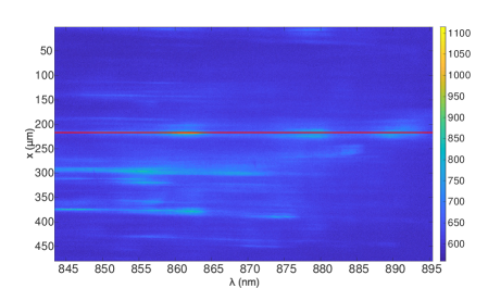
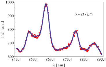
Figure 1: (a) Instance of an intensity spectrum vs position and wavelength. (b) Instance of multi-Gaussian interpolation of the intensity spectrum of GaAs crystal powder in a single $10$ms data acquisition time ($100$ shots) at coordinate $x=217~{}\mu$m, corresponding to the red section in (a). The minimal number $N_{G}$ of Gaussian curves used is determined by the interpolating set yielding the least Akaike parameter. Depending on the $x$ coordinate, $N_{G}$ turns out to vary between $5$ and $10$ [see Supplementary information].

Strong correlation discrimination

Of each set of intensity peaks we compute the normalized fourth order cumulants of their intensities $c_{4}(\omega_{j},\omega_{k},\omega_{l},\omega_{m})$, cf. Methods. Since there are many spurious effects that may contribute to a correlation among modes, in order to identify anomalously large correlations we need a reference for the background correlation.

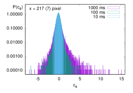
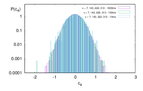
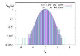
Figure 2: Normalized distribution of $c_{4}$ for acquisition times $10$, $100$, $1000$ ms. (a) $c_{4}$ taken at the same shot, same $x=210~{}\mu$m. (b) $c_{4}$ taken at the same shot, but different positions $x$. (c) $c_{4}$ taken at the different shots, same $x$.

One can observe that the largest correlation values (in the tails of the distributions) turn out to be attained always on those sets whose resonances taken at the same time overlap in the $x$ position (SOIR), with respect to NOIR and background correlations. Moreover, comparing the distributions in Fig. 2 as the number of acquired emissions increases, the dominion of possible values for the SOIR correlations extends its extremes in the low probability tails. This is not the case, on the contrary, for NOIR and background $c_{4}$, insensitive to the change in acquisition time. We, thus, compute three kinds of multi-point correlations:

• SOIR, the correlations of all quadruplets composed by possibly spatially self overlapping intensity resonances, i.e., occurring at the same planar position $x$;

• NOIR, the correlations quadruplets composed by non overlapping intensity resonances, i.e., occurring at well distinct $x$ positions in the same spectral data acquisition;

• BG, the background correlations among resonances pertaining to different spectra, i.e., acquired after different pump shots.

In Fig. 2 (a) we display the probability distributions of the SOIR four-point correlation functions $c_{4}$ for $100$, $1000$ and $10000$ shots. Sets of SOIR are candidate to be nonlinearly interacting. In the center panel of Fig. 2 we display the NOIR $c_{4}$. The latter set might still be composed by interacting modes in an extended mode scenario Fallert09 . Finally, in the right panel of Fig. 2 the BG $c_{4}$ are plotted.

With high confidence, we, finally, operatively identify nonlinearly interacting sets of modes as those whose multi-mode correlation is larger - in absolute value - than the $3\sigma$ of the background correlation distribution. In Fig. 3 we superimpose instances of the normalized distributions for the background, the NOIR and the SOIR correlations for an acquisition time of $100$ ms, clearly showing that the tails of the SOIR extend well beyond the $3\,\sigma$ of the other two.

The presence of these interacting sets of modes is our first result: spatially overlapping modes interact nonlinearly in the random lasing regime.

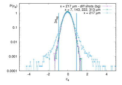
Figure 3: Normalized distributions of $c_{4}$ at acquisition time $100$ ms for background correlations, non-overlapping resonance correlations and spatial overlapping resonance correlations. The vertical lines correspond to $\pm 3\sigma$ of the background correlation distribution.

Frequency matching role in strongly correlated modes

Eventually, we are interested in testing whether the frequencies of interacting modes satisfy FMC. This is indeed, a signature for self-starting mode-locking in the GaAs random laser. To make FMC quantitative, cf. Eq. (2), we introduce a “FMC parameter” against which we can straightforward test multi-mode correlations. In the case of the $4$-mode correlation, taking for illustrative purpose modes $1,2,3$ and $4$, this is

$$\Delta_{4}\equiv\frac{|\omega_{1}-\omega_{2}+\omega_{3}-\omega_{4}|}{\gamma_{1}+\gamma_{2}+\gamma_{3}+\gamma_{4}}$$ (4)

In Fig. 4 the mean square displacement $\sigma_{c_{4}}$ of the correlations among modes within a given $\Delta_{4}$ interval are displayed. For correlations computed from a series of $1000$ spectra, each one acquired in $100$ ms, we plot $\sigma_{c_{4}}$ the distributions of the SOIR, of the NOIR and of the background correlations. It can be observed that no dependence on $\Delta_{4}$ is shown for BG and NOIR correlations. On the contrary, the $\sigma_{c_{4}}$’s of SOIR correlation distributions depend on $\Delta_{4}$. In particular, non-trivially strong correlations only occur among the SOIR, and only for small $\Delta_{4}$, signaling that in those sets of modes - those most probably coupled - their interaction strength depends on how well FMC is satisfied.

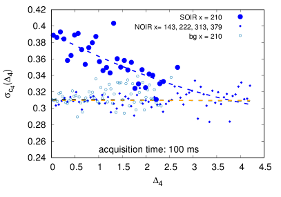
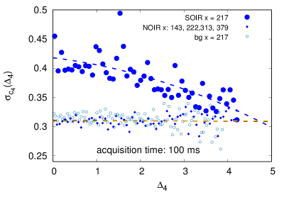
Figure 4: Mean square displacement of the four-point correlation $c_{4}$ values vs. $\Delta_{4}$ at $100$ ms acquisition time for background correlation (bg), non-overlapping resonances and space-overlapping resonances. Left: at pixel $x=210(7)~{}\mu$m. Right: $x=217(7)~{}\mu$m.

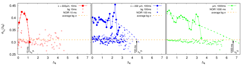
Figure 5: Mean square displacements $\sigma_{c_{4}}$ of the distributions of four-resonance correlation values $c_{4}$ at fixed $\Delta_{4}$ intervals. For SOIR quadruplets at $x=222~{}\mu$m we use large full points, for instances of background (non-iteracting) quadruplets we use small empty points and for the instances of NOIR quadruplets small full points. The $\sigma_{c_{4}}$’s are plotted versus the FMC parameter $\Delta_{4}$ for acquisition times $10$, $100$ and $1000$ ms, corresponding to a spectral integration over, respectively, $100$ (red), $1000$ (blue) and $10000$ (green) pumping shots. Dashed lines are parabolic interpolations of SOIR $\sigma(\Delta)$ behaviors. Background and NOIR correlations do not show any dependence on FMC, whereas SOIR correlation distributions, with large tails at $\Delta_{4}\simeq 0$ corresponding to interacting sets, tend to shrink as the FMC is progressively relaxed. The boundary value $\Delta_{4}^{{\rm ML}}$ at which SOIR $\sigma$’s decreases to values of the order of background $\sigma$’s depends on the acquisition time. In particular, $\Delta_{4}^{{\rm ML}}$ decreases with the number of shots, towards the expected limit of $\Delta_{4}^{{\rm ML}}\lesssim 1$ for a single shot.

This behavior occurs at all acquisition times used in experiments, as it can be observed in Fig. 5. In particular, one can observe that, decreasing the acquisition time, i.e., decreasing the number of recorded photon emissions after each pumping laser shot, the threshold value of $\Delta^{\rm ML}_{4}$ below which surely interacting modes can be neatly discriminated from background correlation decreases.

Ideally, to analyse mode-locking, for every single shot one would like to have the intensity of emission measured as a function of space $(x,y)$ in the sample plane, to control the spatial overlap, and contemporarily resolved in angular frequency $\omega$, to check the FMC, Eq. (2).

Although the integration over many shots (the emission intensity is too low to allow the resolution of the energy-space emission map of a single shot experiment), we can clearly observe the shrinking of $\Delta^{\rm ML}_{4}$ with decreasing number of shots, consistently with the upper theoretical limit of $\Delta^{\rm th}_{4}=1$ for single shot experiments.

The evidence that only SOIR show $\Delta$-dependent correlations is a clear indication of the onset of nonlinear mode-locking in random lasers and our main result: sets of modes satisfying FMC are much strongly correlated than sets of modes not satisfying FMC. The former non-trivially large correlations is to be accounted for by the interaction of the modes. The latter cannot be distinguished from $\Delta$-independent background correlations.

Discussion

In the present work we considered multi-mode correlations among spatially overlapping intensity resonances (SOIR), spatially non-overlapping intensity resonances (NOIR) and background correlations among resonances in independent spectra (BG). Firstly, by compared analysis of sets of background correlations and correlations among NOIR we cannot appreciate any difference in the behavior of their distributions, as reported in Figs. 2 and 3. Since correlations among NOIR are not any larger than background correlations we cannot discriminate possible long-range non-linear mode-coupling with respect to noise.

This is not the case for SOIR multi-point correlations. Calibrating $P_{{\rm SOIR}}(c_{4})$ by means of the background correlation distributions, we identify interacting quadruplets as those composed by modes whose intensity fluctuations correlation lies in the tails of their distribution, actually extending beyond $3~{}\sigma_{{\rm BG}}$ of the Gaussian interpolation of the $c_{4}$ BG distribution, as shown in Fig. 3.

The same behavior is found also if we change the pumping power, as far as the random laser is above threshold and clear resonances can be distinguished in the space-energy spectrum (Supplementary information).

As observed in Section Results, cf. Figs. 4, 5, the frequency matching condition, Eq. (2), appears to play a determinant role in the distribution of the $c_{4}$ values of interacting set of modes. Moreover, we observe that the shorter the acquisition time, the smaller the range of values of $\Delta_{4}$ at which large correlation occurs. According to Eq. (2), interaction between modes would be allowed only to modes whose energies satisfy the FMC relationship. In terms of data reported in Figs. 5 this would imply that interacting mode sets should appear for $\Delta\lesssim O(1)$. Given the statistical nature of (i) the modes identification and (ii) the interaction recognition from anomalously large multi-point correlations, the outcome is strongly compatible with such a requirement.

This observation is a strong evidence in favour of the occurrence of mode-locking in random lasers, that is, the same mechanisms behind the nonlinear mode coupling in standard, ordered, multimode lasers, though without any ad hoc device like a saturable absorber or a modulator. It is a self-starting mechanism induced by randomness.

As a last remark we recall that in the ordered case mode-locking is responsible for ultra-fast pulses. On the contrary in random lasers, no train of pulses is present, because the distribution of frequencies is random, rather than comb-like Udem02 , preventing the rise of a pulse even in presence of frequency matching and phase-locking. Indeed, the Fourier transform in time does not produce a modulated signal with a short envelope Marruzzo15 . Actually, also in presence of almost equispaced resonances it would be extremely difficult to identify a pulse shorter than the pumping laser pulse and, in the subclass of optically random media displaying glassy random lasers, this might not be feasible at all Gradenigo19 . To unveil the self-starting mechanism beyond the just demonstrated locking of modes in random lasers mandatorily requires the identification of mode phases. We believe that the presented results might be a significant step to stimulate and lead the theoretical understanding and the experimental procedures necessary to provide a protocol to determine mode phases in random lasers.

Materials and Methods

Samples

The sample is made by grinding a piece of GaAs wafer - bathed in methanol - in a pestle and mortar, in order to obtain a paste with grain typically smaller than $10~{}\mu$m. The resulting paste is then highly diluted in methanol and deposited by drop casting on a glass substrate. During the deposition, the glass substrate is placed on a heater to have a fast evaporation of the solvent. The packing density and sample thickness is increased by repeating $50$ times the drop casting process. Obviously, the sample is highly inhomogeneous. However, the thickness never exceeds $100~{}\mu$m. A second glass slide covers the sample, which is finally sealed with parafilm on the sides.

Experimental setup and measurements

The laser source is a $30$ fs pulsed laser at $780$ nm with repetition rate $10$ KHz. The excitation line is orthogonal to the sample surface, while the detection line is along the opposite side of the sample (i. e., transmission configuration). Adjusting the spot size and excitation power, we can roughly control the number of active random lasers loops. The Gaussian spot size is tuned to about $300~{}\mu$m (FWHM); this spot size guarantees a total number of emitters that are easily distinguishable when the real space emission map is projected on the CCD camera. The detection line consists of two plano convex lenses projecting the sample plane at the spectrometer entrance (so in focus on the CCD camera). The spectrometer slits aperture allows the selection of a vertical slice of the emission space map and the energy resolution of the emission spectrum. The experiments have been performed with a slit aperture corresponding to $10~{}\mu$m horizontal selection on the sample surface, in order to have the selection of a single emitter along the horizontal axis. The overall numerical aperture of the detection line is $0.64$.

Multi-point correlation definition

The fourth order connected correlation function of intensity peaks $I_{j}(\omega_{j})$ reads:

$$C_{4}(\omega_{j},\omega_{k},\omega_{l},\omega_{m}) = \langle I_{j}I_{k}I_{l}I_{m}\rangle-\langle I_{j}I_{k}I_{l}\rangle\langle I_{m}\rangle-\langle I_{j}I_{k}I_{m}\rangle\langle I_{l}\rangle-\langle I_{j}I_{m}I_{l}\rangle\langle I_{k}\rangle-\langle I_{m}I_{k}I_{l}\rangle\langle I_{j}\rangle$$

$$-\langle I_{j}I_{k}\rangle\langle I_{l}I_{m}\rangle-\langle I_{j}I_{l}\rangle\langle I_{k}I_{m}\rangle-\langle I_{j}I_{m}\rangle\langle I_{k}I_{l}\rangle+2\langle I_{j}I_{k}\rangle\langle I_{l}\rangle\langle I_{m}\rangle+2\langle I_{j}I_{l}\rangle\langle I_{k}\rangle\langle I_{m}\rangle$$

$$+2\langle I_{j}I_{m}\rangle\langle I_{k}\rangle\langle I_{l}\rangle+2\langle I_{k}I_{l}\rangle\langle I_{j}\rangle\langle I_{m}\rangle+2\langle I_{k}I_{m}\rangle\langle I_{j}\rangle\langle I_{l}\rangle+2\langle I_{l}I_{m}\rangle\langle I_{j}\rangle\langle I_{k}\rangle-6\langle I_{j}\rangle\langle I_{k}\rangle\langle I_{l}\rangle\langle I_{m}\rangle$$

where the average is taken over the statistical sample of all the combinations of the same set of modes displayed in experiments at fixed external condition and stable pumping. We, further, normalize $C_{4}$ to the mean square displacements of the intensities of the modes, i.e.,

$$c_{4}(\omega_{j},\omega_{k},\omega_{l},\omega_{m}) \equiv \frac{C_{4}(\omega_{j},\omega_{k},\omega_{l},\omega_{m})}{\sigma_{j}(\omega_{j})\sigma_{k}(\omega_{k})\sigma_{l}(\omega_{l})\sigma_{m}(\omega_{m})}$$

$$\sigma_{j}(\omega_{j}) = \sqrt{\langle\left(I_{j}-\langle I_{j}\rangle\right)^{2}\rangle}$$

Supplementary materials

.1 Theoretical modeling

The dynamics of the electromagnetic field is suitably expressed in the slow mode decomposition

$$\bm{E}(\bm{r},t)=\sum_{k}a_{k}(t)e^{\imath\omega t}\bm{E}_{k}(\bm{r})+\mbox{c.c.}$$ (5)

where the modes $\bm{E}_{k}(\bm{r})$ of angular frequency $\omega_{k}$ are such that their complex amplitudes $a(t)$ evolve slowly with respect to $\omega^{-1}$ and follow a nonlinear stochastic dynamics. In standard mode-locked lasers with passive mode-locking induced by a saturable absorber, e. g., the phasors dynamics is given by the so-called Haus master equation Haus00 , that, in the angular frequency domain Gordon02 , reads:

$$\dot{a}_{k_{1}}(t)=(g_{k_{1}}-\ell_{k_{1}}+\imath D_{k_{1}})a_{k_{1}}(t)+(\gamma+i\delta)\sum_{k_{2}k_{3}k_{4}}^{{\rm FMC}}a_{k_{2}}(t)a_{k_{3}}^{*}(t)a_{k_{4}}(t)+\eta_{k_{1}}(t)$$ (6)

where $g_{k}$, $\ell_{k}$ and $D_{k}$ are, respectively, the frequency-dependent components of the gain, the loss and the dispersion velocity. In the case of passive mode-locking, the real part of the non-linear coefficient $\gamma$ represents the self-amplitude modulation coefficient of the saturable absorber and the imaginary part $\delta$ represents the coefficient of the self-phase-modulation caused by the Kerr-effect. The acronym FMC on sums stays for Frequency Matching Condition, cf. Tab. 1 and Eq. (2)${}_{\text{MT}}$ in the main text, arising in the approach leading to the master equation (6), after averaging out single mode’s fast oscillations $\sim e^{\imath\omega_{n}t}$ Haus00 ; Gordon02 ; Gat04 ; Katz06 ; Antenucci15c ; Antenucci15d ; Antenucci15b . The white noise $\eta_{n}(t)$ is a stochastic variable representing the contribution of spontaneous emission, linked to the thermal kinetic energy of the atoms through its covariance

$$\langle\eta_{k}(t)\eta_{n}(t^{\prime})\rangle\propto T\delta_{kn}\delta(t-t^{\prime})$$ (7)

where $T$ is the temperature. For arbitrary spatial distribution of modes $\bm{E}(\bm{r})$ and heterogeneous susceptibility, i.e., when the system is intrinsically random, starting from quantum dynamical Jaynes-Cumming equations, downgrading from quantum creation-annihilation operators to classical complex-valued amplitudes, taking into account spontaneous emission and gain saturation, a generalized phasor dynamic equation is recovered for random lasers Antenucci16 :

$$\dot{a}_{k_{1}}(t)=\sum_{k_{2}}^{{\rm FMC}}g_{k_{1}k_{2}}^{(2)}a_{k_{2}}(t)+\sum_{k_{2}k_{3}k_{4}}^{{\rm FMC}}g_{k_{1}k_{2}k_{3}k_{4}}^{(4)}~{}a_{k_{2}}(t)a_{k_{3}}^{*}(t)a_{k_{4}}(t)+\eta_{k_{1}}(t)$$ (8)

where we have considered only the first nonlinear term satisfying time reversal symmetry in the electromagnetic phasor’s dynamics. Further terms would only perturbatively modify the leading behavior of the fourth order term. Odd terms like those related to the $\chi^{(2)}$ optical susceptibility, occurring in non-centrometric potentials, can also be included theoretically but practically will play no role because of the usually limited wavelength dominion in the intensity spectra of the random lasers . The complexity of the mode interaction is hidden inside the $g$ coefficients in Eq. (3)${}_{\text{MT}}$ of the main text. Finally, recognizing in Eq. (8) a potential Langevin equation, the effective phasor Hamiltonian of Eq. (1)${}_{\text{MT}}$ in the main text is derived.

$\#$ $\omega$’s	indices	FMC
$2$	$\mathbf{k}_{2}\equiv{k_{1},k_{2}}$	$|\omega_{k_{1}}-\omega_{k_{2}}|<\gamma_{k_{1}}+\gamma_{k_{2}}$
$3$	$\mathbf{k}_{3}={k_{1},k_{2},k_{3}}$	$|2\omega_{k_{1}}-\omega_{k_{2}}-\omega_{k_{3}}|<2\gamma_{k_{1}}+\gamma_{k_{2}}+\gamma_{k_{3}}$
$4$	$\mathbf{k}_{4}={k_{1},k_{2},k_{3},k_{4}}$	$\left.\begin{array}[]{c}|\omega_{k_{1}}-\omega_{k_{2}}+\omega_{k_{3}}-\omega_{k_{4}}|\\ |\omega_{k_{2}}-\omega_{k_{1}}+\omega_{k_{3}}-\omega_{k_{4}}|\\ |\omega_{k_{1}}-\omega_{k_{3}}+\omega_{k_{2}}-\omega_{k_{4}}|\end{array}\right\}<\gamma_{k_{1}}+\gamma_{k_{2}}+\gamma_{k_{3}}+\gamma_{k_{4}}$

Table 1: Summary of all possible FMC’s for modes interacting via Eq. (1). Pairwise, three- and four-body terms are reported.

.2 Observable definitions and data analysis

Identification of the intensity peaks of the modes by multi Gaussian interpolation

We herewith describe the fitting procedure composing the resonances identification step in Section Results in the main text. In a first series of measurements, because of a large refinement in energy with respect to the behavior of emission spectra, we have first coarse-grained the position-energy grid binning four pixels in the $\lambda$ direction. This corresponds to a resolution of $0.15$ nm in the wavelength (and $1.2\mu$m in position). We have $335$ pixels in the wavelength direction, with the lowest extreme being $\lambda=843.4116$ nm and the total spectral width amounting to $52.0075$ nm. Considering an approximately constant spacing $\Delta\lambda$, this means that

$$\lambda[\mbox{nm}]=52.0075/334*(\mbox{pixel}-1)+843.4116\quad;\qquad\mbox{pixel}\in[1:335]$$ (9)

In the second series of experiments the wavelength pixels are only $672$, with resolution already of $0.149$ nm (and $0.9$ $\mu$m in position) and there was no need for binning.

We, then performed multi-Gaussian interpolations of spectra $I(x;\lambda)$ at fixed position $x=1,\ldots,N_{x}$. We denote the number of Gaussians employed by $N_{G}$ and we estimate two parameters for each Gaussian $n=1,\ldots,N_{G}$, mean $\bar{\lambda}_{n}$ and variance $\sigma_{n}^{2}$, as well as a relative weight $w_{n}$, for a total number of parameters $K=3N_{G}$. At each position $x$, and for each $N_{G}$, we compute the log-likelihood

$$\ln\mathcal{L}\left(\lambda|\{w_{n}\},\{\bar{\lambda}_{n}\},\{\sigma_{n}\}\right)=\ln\sum_{n=1}^{N_{G}}w_{n}\exp\left[-\frac{\left(\lambda-\bar{\lambda}_{n}\right)^{2}}{2\sigma_{n}^{2}}\right]$$ (10)

The best fit at each $x$ is the one whose parameter estimators for $\{w_{n},\bar{\lambda}_{n},\sigma_{n}\}$ maximize the log-likelihood $\ln{\cal L}$ or, equivalently, minimize the so-called the Akaike parameter

$$A=2K-2\ln{\cal L}$$

built with the least number of Gaussians. i.e., the least $K$. This is the Akaike Information Criterion to avoid overfitting and underfitting.

To each experiment $t$ of the series, a grid of mode intensities is associated: $I^{(t)}(x,\Delta x;\lambda;\Delta\lambda)$, where $\Delta x$ and $\Delta\lambda$ are the Full Width Half Maximum of the interpolated distributions around, respectively, $x$ and $\lambda$ ($\Delta\lambda_{n}=2\sqrt{2\ln 2}\sigma_{n}$).

We consider the same single mode $n$ as present in the spectra of two different experiments $t_{A}$ and $t_{B}$ of the series if

$$x_{n}^{\{t_{A}\}}=x_{n}^{\{t_{B}\}}$$

$$|\lambda_{n}^{\{t_{A}\}}-\lambda_{n}^{\{t_{B}\}}|<\delta\lambda$$

$$2\frac{\Delta\lambda_{n}^{A}-\Delta\lambda_{n}^{B}}{\Delta\lambda_{n}^{A}+\Delta\lambda_{n}^{B}}<\bar{\delta}\lambda$$

where the absolute and relative uncertainties $\delta\lambda$ and $\bar{\delta}\lambda$ are chosen depending on the resolution required. $\Delta x$ is not considered in the analysis but it is of the order of 6 pixels. I. e., 7 ${\mu}$m in the first series of experiments and $4$ $\mu$m in the second one.

In both series of experiments we used $\delta\lambda=1.5$ nm and $\bar{\delta}\lambda=0.1$. For spectra of lower resolution and less intense peaks we also considered a rougher coarse graining, where two parameters in the mode identification are $\delta\lambda=4.5$ nm and $\bar{\delta}\lambda=0.3$. We resorted to this less precise approximation exclusively when the modes’ statistics is too low to provide clear behaviors of the distributions of $c_{4}$ values. This is the case, e.g., in some of the data with acquisition time of $10$ ms and low pumping energy in the second series of experiments (see Sec. .4).

Localization of resonances in the monochromator vertical direction $y$

Having nearby $x$ coordinates for the modes is a necessary condition to have spatial overlap of the intensity peaks. Indeed, mode’s extensions should also overlap in the $y$ direction, the horizontal direction of the slit, and in the $z$ direction, the thickness of the sample. Knowing the total range in $y$ and $z$, we can estimate the probability that if four modes have the same $x$ they will be effectively mutually overlapping also in $y$ and $z$. Let us call $L_{y}$ the total $y$-range, equal to the slit opening ($L_{y}\simeq 10~{}\mu$m) and $\Delta\equiv\Delta y\simeq\Delta x=7~{}\mu$m the typical extension of the most peaked resonances that we analyzed. Let us, then, take as indicative average depth of the sample $L_{z}\simeq 50~{}\mu$m, the total $z$-range. The probability that four modes of roughly the same extension $\Delta$ at the same $x$ share a non-zero spatial intersection along the $y$ (or $z$) coordinate, in a total range $L_{y}$ (or $L_{z}$) (enough larger than $\Delta$), can be estimated as

$$p_{4}^{(y,z)}(\Delta_{w},L_{w}) = 8\frac{\Delta_{w}^{3}}{L_{w}^{3}};\qquad\qquad w=y,z$$ (11)

This is independent from the coordinates of the modes. For the setup and the sample we used the probability of having a four mode overlap at given $x$ position is, thus,

$$p_{4}^{(x)}=p_{4}^{(y)}(7,10)\times p_{4}(7,50)\simeq 0.060$$ (12)

This means that once we know that four resonances at different wavelength of the acquired spectra are at the same point $x$, they will be actually overlapping in 3D space only a fraction $p_{4}^{(x)}$ of the times. In the results shown in this paper, we always have at least $\sim 100$ quadruplets of resonant modes at given $x$ coordinate, so that we can expect with high probability that in all cases there are at least few spatially overlapping sets for all the cases shown. At the same time, the fact that the probability of overlapping is relatively low ($\lesssim 10\%$) explains the presence of many low-interacting sets even in the SOIR setup and makes our analysis of the background correlations essential to extract the signal coming from the few spatially overlapping sets.

.3 Multi-set mode correlation vs. statistics

We further considered how finite sample size may affect the results shown in paper. In particular, note that typically the number of possible quadruplets decreases rapidly as a function of $\Delta_{4}$. We therefore performed a further test to verify whether a high (low) correlation $c_{4}$ at a given $\Delta_{4}$ value might be related to the presence of a large (small) number $N_{q}$ of sets of modes for the same frequency combination $\Delta_{4}$. In Fig. 6 the rescaled histograms of $N_{q}$ as function of $\Delta_{4}$ are plotted together with the average value of the modulus of the correlation $|c_{4}|$ at the same $\Delta_{4}$: no special correlation can be observed.

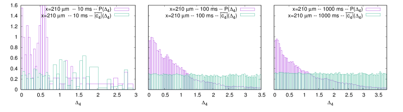
Figure 6: Normalized histogram $P_{q}(\Delta_{4})$ of the number of SOIR quadruplets (at position $x=210~{}\mu$m) whose frequencies yield a given $\Delta_{4}$ compared to a average value of the modulus of the correlation $c_{4}$.

To be quantitative, we, further, computed the Pearson correlation coefficient $r$ between $\overline{|c_{4}(\Delta_{4})|}$ and $N_{q}(\Delta_{4})$ for both the SOIR and NOIR cases, as reported in Fig. 7. We stress that the NOIR correlations are typically evaluated on a much larger number of quadruplets than the SOIR ones, as in the former case one considers all possible quadruplets among modes in four different positions while in the latter only among modes at one fixed position. The BG correlations are instead always evaluated with the same statistics as the SOIR ones at the same position, for an easier comparison. We observe that the value of $r$ is (i) always relatively small $\lesssim 0.3$, (ii) without a definite value over different experiments and (iii) of the same order of magnitude in the two cases SOIR and NOIR. This observation reinforces the conclusions of the previous sections, showing that our result of a dependency of $c_{4}$ from $\Delta_{4}$ cannot be explained as a small sample size effect.

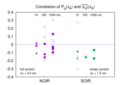
Figure 7: Pearson correlation between the average $\overline{|c_{4}(\Delta_{4})|}$ of the four-point correlation values and the number of quadruplets $P_{q}(\Delta_{4})$ over which the correlations are computed. Values obtained using data from NOIR and SOIR quadruplets are compared. Outcome from experimental series at well different acquisition times ($10,100,1000$ ms) are reported. We repeated the analysis in two different cases for the identification of the single peaks (see Methods): with $\Delta\lambda=4.5$ nm and one with $\Delta\lambda=1.5$ nm.

.4 Mode-locking dependence on pumping power

Eventually we have carried out our analysis on the same sample for different powers of the pump laser and explored if and how non-linear mode-coupling depends on pumping. In Fig. 8 we compare the probability distributions of the background 4-peak correlations and the SOIR correlations at given resonance locations at two different pumping powers, $25$ and $60$ mW. The same effect of long tails and non Gaussianity is observed at all powers for which clear intensity resonances can be resolved in space and wavelength and, once the mode resonances are there, no further dependence on the external power is observed.

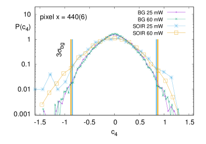
Figure 8: Comparison between $P(c_{4})$ of SOIR and BG correlations at different pumping power $P=25$ mW and $60$ mW at the same resonance at the same point $x=400(5)~{}\mu$m for acquisition time $100$ ms (1000 shots). At both powers the SOIR distributions have wider tails than the background ones. Both distributions do not appear to change with the pumping power.

References

Ackowledgements

The authors thank D. Ancora, G. Gradenigo, M. Leonetti, A. Marruzzo for useful discussions. The research leading to these results has received funding from the Italian Ministry of Education, University and Research under the PRIN2015 program, grant code 2015K7KK8L-005 and the European Research Council (ERC) under the European Union’s Horizon 2020 research and innovation program, project ElecOpteR Grant Agreement No. 780757 and project LoTGlasSy, Grant Agreement No. 694925.

Author contributions G.L. and B.S.F. performed the measurements on the random lasers; G.L. prepared the samples; G.L. and D.S. designed the experimental setup; D.S. coordinated the experimental work; F.A. and L.L. proposed the theoretical framework and performed the data analysis; L.L.. prepared the manuscript with input from F.A., D.S. and G.L. All authors contributed to the discussion of the data and to the final draft of the manuscript.

Competing financial interests

The authors declare no competing financial interests.

References

- (1) Cao, H. et al. Random laser action in semiconductor powder. Phys. Rev. Lett. 82, 2278 (1999).
- (2) Cao, H. Lasing in random media. Waves in Random Media and Complex Media 13, R1–R39 (2003).
- (3) Wiersma, D. S. The physics and applications of random lasers. Nature Physics 4, 359 (2008).
- (4) Andreasen, J. et al. Modes of random lasers. Adv. Optics and Photonics 3, 88–127 (2011).
- (5) Cao, H. et al. Ultraviolet lasing in resonators formed by scattering in semiconductor polycrystalline films. Appl. Phys. Lett. 73, 3656 (1998).
- (6) Anni, M. et al. Modes interaction and light transport in bidimensional organic random lasers in the weak scattering limit. Phys. Rev. B 70, 195216 (2004).
- (7) Cao, H., Xu, J. Y., Chang, S. H. & Ho, S. T. Transition from amplified spontaneous emission to laser action in strongly scattering media. Phys. Rev. E 61, 1985 (2000).
- (8) van der Molen, K. L., Mosk, A. P. & Lagendijk, A. Intrinsic intensity fluctuations in random lasers. Phys. Rev. A 74, 053808 (2006).
- (9) van der Molen, K. L., Tjerkstra, R. W., Mosk, A. P. & Lagendijk, A. Spatial extent of random laser modes. Phys. Rev. Lett. 98, 143901 (2007).
- (10) El-Dardiry, R. G. S., Mosk, A. P., Muskens, O. L. & Lagendijk, A. Experimental studies on the mode structure of random lasers. Phys. Rev. A 81, 043830 (2010).
- (11) Tulek, A., Polson, R. C. & Vardeny, Z. V. Naturally occurring resonators in random lasing of -conjugated polymer films. Nature Phys. 6, 303 – 310 (2010).
- (12) Anju, K. A., Radhakrishnan, P., Nampoori, V. P. N. & Kailasnath, M. Enhanced random lasing from a colloidal cdse quantum dot-rh6g system. Laser Phys. Lett. 12, 025006 (2015).
- (13) Viola, I., Leuzzi, L., Conti, C. & Ghofraniha, N. Organic Lasers, chap. Basic Physics and Recent Developments of Organic Random Lasers (Pan Stanford, 2018).
- (14) Haus, H. A. Mode-locking of lasers. IEEE J. Quantum Electron. 6, 1173–1185 (2000).
- (15) Antenucci, F., Conti, C., Crisanti, A. & Leuzzi, L. General phase diagram of multimodal ordered and disordered lasers in closed and open cavities. Phys. Rev. Lett. 114, 043901 (2015).
- (16) Antenucci, F., Crisanti, A. & Leuzzi, L. Complex spherical 2+4 spin glass: A model for nonlinear optics in random media. Phys. Rev. A 91, 053816 (2015).
- (17) Antenucci, F. Statistical physics of wave interactions (Springer, 2016).
- (18) Leonetti, M., Conti, C. & Lopez, C. The mode-locking transition of random lasers. Nat. Photon. 5, 615 (2015).
- (19) Marruzzo, A. & Leuzzi, L. Nonlinear xy and p-clock models on sparse random graphs: Mode-locking transition of localized waves. Phys. Rev. B 91, 054201 (2015).
- (20) Antenucci, F., Ibáñez Berganza, M. & Leuzzi, L. Statistical physical theory of mode-locking laser generation with a frequency comb. Phys. Rev. A 91, 043811 (2015).
- (21) Gordon, A. & Fischer, B. Phase transition theory of many-mode ordering and pulse formation in lasers. Phys. Rev. Lett. 89, 103901 (2002).
- (22) Gat, O., Gordon, A. & Fischer, B. Solution of a statistical mechanics model for pulse formation in lasers. Phys. Rev. E 70, 046108 (2004).
- (23) Udem, T., Holzwarth, R. & Hansch, T. Optical frequency metrology. Nature 416, 233 (2002).
- (24) Baltus̃ka, A. et al. Attosecond control of electronic processes by intense light fields. Nature 421, 611 (2003).
- (25) Schliesser, A., Gohle, C., Udem, T. & Hänsch, T. W. Complete characterization of a broadband high-finesse cavity using an optical frequency comb. Optics Express 14, 5975 (2006).
- (26) Lethokov, V. S. Generation of light by a scattering medium with negative resonance absorption. Sov. Phys. JETP 26, 835 (1968).
- (27) Soukoulis, C. M., Jiang, X., Xu, J. X. & Cao, H. Dynamic response and relaxation oscillations in random lasers. Phys. Rev. B 65, 041103R (2002).
- (28) Gradenigo, G., Antenucci, F. & Leuzzi, L. Glass transition and lack of equipartition in a statistical mechanics model for random lasers (2019). eprint arXiv:1902.00111v1.
- (29) Antenucci, F., Crisanti, A. & Leuzzi, L. The glassy random laser: replica symmetry breaking in the intensity fluctuations of emission spectra. Scientific Reports 5, 16792 (2015).
- (30) Marruzzo, A. & Leuzzi, L. Multi-body quenched disordered and -clock models on random graphs. Phys. Rev. B 93, 094206 (2016).
- (31) Akaike, H. A new look at the statistical model identification. IEEE Transactions on Automatic Control 19, 716?723 (1974).
- (32) Fallert, J. et al. Co-existence of strongly and weakly localized random laser modes. Nat. Photon. 3, 279–282 (2009).
- (33) Katz, M., Gordon, A., Gat, O. & Fischer, B. Statistical theory of passive mode locking with general dispersion and kerr effect. Phys. Rev. Lett. 97, 113902 (2006).
- (34) Antenucci, F., Ibañez Berganza, M. & Leuzzi, L. Statistical physics of nonlinear wave interaction. Phys. Rev. B 92, 014204 (2015).