Certifying polynomial non-negativity
via hyperbolic optimization

Abstract

We describe a new approach to certifying the global nonnegativity of multivariate polynomials by solving hyperbolic optimization problems—a class of convex optimization problems that generalize semidefinite programs. We show how to produce families of nonnegative polynomials (which we call hyperbolic certificates of nonnegativity) from any hyperbolic polynomial. We investigate the pairs $(n,d)$ for which there is a hyperbolic polynomial of degree $d$ in $n$ variables such that an associated hyperbolic certificate of nonnegativity is not a sum of squares. If $d\geq 4$ we show that this occurs whenever $n\geq 4$. In the degree three case, we find an explicit hyperbolic cubic in $43$ variables that gives hyperbolic certificates that are not sums of squares. As a corollary, we obtain the first known hyperbolic cubic no power of which has a definite determinantal representation. Our approach also allows us to show that, given a cubic $p$, and a direction $e$, the decision problem “Is $p$ hyperbolic with respect to $e$?” is co-NP hard.

1 Introduction

The problem of deciding nonnegativity of a multivariate polynomial is central to solving optimization and feasibility problems expressed in terms of polynomials. These, in turn, arise naturally in a wide range of applications including control systems and robotics, combinatorial optimization, game theory, and quantum information (see Section 1.2 for further discussion, and the edited volume [BPT12] for an introduction to these ideas).

One of the benefits of a polynomial formulation of an optimization problem is that one can then construct a hierarchy of more tractable ‘relaxations’ of the problem, based on the fact that being a sum of squares of polynomials is a sufficient condition for a polynomial to be nonnegative. Deciding whether a polynomial is a sum of squares can be formulated as a semidefinite programming feasibility problem [Sho87, Nes00, Par03, Las01]. While such semidefinite programming-based relaxations of semialgebraic problems have proven very useful for a range of problems, there has been notable recent progress (both qualitative [Sch18] and quantitative [LRS15]) demonstrating the limitations of this approach.

Hyperbolic optimization problems (or hyperbolic programs) are a family of convex optimization problems that generalize semidefinite optimization problems [Gül97]. These involve maximizing a linear functional over the intersection of an affine subspace and a hyperbolicity cone (a convex cone constructed from a hyperbolic polynomial, which is a multivariate polynomial with certain real-rootedness properties that we define precisely in Section 2). Hyperbolic programs enjoy many of the good algorithmic properties of semidefinite programs [Gül97]. Despite this, algorithms for hyperbolic programming are less mature than those for semidefinite programming. Indeed, much of the recent research on hyperbolic programming has focused on trying to reformulate various classes of hyperbolic programs as semidefinite programs, or on related geometric questions associated with the ‘generalized Lax conjecture’ and its variants [Ami19, Brä14, KPV15, SP15, Sau18]. This lack of algorithmic development may be the result of not having generic ways to produce hyperbolic programming-based formulations and/or relaxations of polynomial optimization problems, beyond those already captured by sums of squares.

This paper introduces ways to construct families of nonnegative polynomials that can be searched over via hyperbolic optimization. We call these hyperbolic certificates of nonnegativity. By appropriately choosing the data that specify such a family of nonnegative polynomials, we can recover sums of squares certificates of nonnegativity. As such, using the ideas in this paper, we could construct hyperbolic programming-based relaxations of polynomial feasibility and optimization problems by replacing sums of squares relaxations with relaxations based on hyperbolic certificates of nonnegativity. One significant challenge, not addressed in this paper, is that many choices need to be made to specify a family of hyperbolic certificates of nonnegativity. Given a specific structured class of polynomial optimization problems, it is currently unclear which choices might be appropriate to obtain strong hyperbolic programming-based relaxations using the framework presented in this paper.

A main focus of the paper is the construction of hyperbolic polynomials for which the associated hyperbolic certificates of nonnegativity are not sums of squares. These are of interest because they have the potential to form the basis of hyperbolic programming-based relaxations of polynomial optimization problems that are stronger than semidefinite programming-based relaxations of comparable complexity.

1.1 Contributions

We now discuss the contributions of the paper in more technical detail, and indicate where the main results appear in the paper.

Hyperbolic certificates of nonnegativity

Given a hyperbolic polynomial $p$ of degree $d$ in $n$ variables and a direction of hyperbolicity $e\in\mathbb{R}^{n}$ (see Section 2.2 for the definition of these terms), we construct a polynomial map

$$(x,y)\mapsto\phi_{p,e}(x,y)[\cdot]$$

from $\mathbb{R}^{n}\times\mathbb{R}^{d}$ to linear functionals on $\mathbb{R}^{n}$ such that $\phi_{p,e}(x,y)[u]\geq 0$ for all $x,y$ if, and only if, $u$ is in the hyperbolicity cone associated with $p$ and $e$ (Theorem 3.7). This slightly extends a related construction due to Kummer, Plaumann, and Vinzant [KPV15].

If $f$ and $g$ are polynomial maps, then $\phi_{p,e}(f(z),g(z))[u]$ is a nonnegative polynomial in $z$ whenever $u$ is in the hyperbolicity cone associated with $p$ and $e$. If a polynomial can be written this way for a choice of hyperbolic polynomial $p$, direction of hyperbolicity $e$, and polynomial maps $f$ and $g$, we say it has a hyperbolic certificate of nonnegativity (see Definition 3.12). We can search for such a description of a polynomial (for fixed $p$, $e$, $f$, and $g$) by solving a hyperbolic optimization problem. Moreover, by appropriately specifying these data, we can recover sums of squares certificates of nonnegativity (Proposition 3.13).

Hyperbolic and SOS-hyperbolic polynomials

If all nonnegative polynomials of the form $\phi_{p,e}(x,y)[u]$ are sums of squares, we say that $p$ is SOS-hyperbolic with respect to $e$ (see Definition 4.2). From the point of view of this paper, we are most interested in hyperbolic polynomials that are not SOS-hyperbolic, since these give rise to tractable families of nonnegative polynomials that go beyond sums of squares.

In Sections 4 and 5 we investigate the degrees $d$, and numbers of variables $n$, for which there is a hyperbolic polynomial that is not SOS-hyperbolic. In Section 4 we characterize when this happens for $d\geq 4$ by showing that the specialized Vámos polynomial,

$$p(x_{1},x_{2},x_{3},x_{4})=x_{3}^{2}x_{4}^{2}+4(x_{1}x_{2}x_{3}+x_{1}x_{2}x_{4}+x_{1}x_{3}x_{4}+x_{2}x_{3}x_{4})(x_{1}+x_{2}+x_{3}+x_{4}),$$

is hyperbolic but not SOS-hyperbolic (Proposition 4.9), and showing how to take a hyperbolic but not SOS-hyperbolic polynomial and increase its number of variables, or its degree, and maintain this property (Propositions 4.10 and 4.13). Variations of the specialized Vámos polynomial have been studied by Brändén [Brä11], Kummer [Kum16], Kummer, Plaumann, and Vinzant [KPV15], Burton, Vinzant, and Youm [BVY14], and Amini and Brändén [AB18]. Notably, [KPV15, Example 5.11] shows that a closely related quartic in five variables is hyperbolic but not SOS-hyperbolic.

In Section 5 we study the case $d=3$, and obtain a partial classification of when hyperbolicity and SOS-hyperbolicity coincide. We show how to construct, from a simple graph, a one-parameter family of cubic polynomials that are hyperbolic if, and only if, the parameter is bounded by the clique number of the graph. This allows us to establish co-NP-hardness of deciding hyperbolicity of cubic polynomials (Theorem 5.4). By choosing $\mathcal{G}=(\mathcal{V},\mathcal{E})$ to be the icosahedral graph, (with $12$ vertices and $30$ edges), we obtain a hyperbolic cubic

$$p(x_{0},x,y)=x_{0}^{3}-3x_{0}\left(\sum_{i\in\mathcal{V}}x_{i}^{2}+\sum_{\{i,j\}\in\mathcal{E}}y_{ij}^{2}\right)+9\sum_{\{i,j\}\in\mathcal{E}}x_{i}x_{j}y_{ij},$$ (1)

in $43=1+12+30$ variables that we show is not SOS-hyperbolic.

The known cases where all hyperbolic polynomials are SOS-hyperbolic occur because, if a power of a polynomial has a definite determinantal representation, then it is SOS-hyperbolic (Proposition 4.7). This is a common generalization of results due to Kummer, Plaumann, and Vinzant [KPV15], and Netzer, Plaumann, and Thom [NPT13]. As such, any hyperbolic polynomial that is not SOS-hyperbolic is a hyperbolic polynomial for which no power has a definite determinantal representation. In particular, the cubic polynomial (1) associated with the icosahedral graph, appears to be the first reported hyperbolic cubic with this property.

Parameterizing the dual cone

The dual cones of hyperbolicity cones are, in general, not well understood. In Section 7 we show that the polynomial map $(x,y)\mapsto\phi_{p,e}(x,y)[\cdot]$ almost (i.e., up to closure) parameterizes the dual of the associated hyperbolicity cone (Theorem 7.2). We then discuss specific situations in which the map exactly parameterizes the closed dual cone, giving new ‘hidden convexity’ results, where the image of a polynomial map is convex.

1.2 Applications via polynomial optimization

We now discuss, in a little more detail, the connection between certifying nonnegativity of polynomials and polynomial optimization, and touch on some of the myriad applications of polynomial optimization.

Polynomial optimization problems involve the minimization of a multivariate polynomial over a set defined by polynomial inequality and equality constraints. By introducing additional variables, one can reduce to the case of minimization over the real points of an algebraic variety $\mathcal{V}$ defined by polynomial equations, i.e.,

$$\textup{minimize}_{z}\;\;q_{0}(z)\;\;\textup{subject to}\;\;z\in\mathcal{V}\cap\mathbb{R}^{n}.$$ (2)

For instance, if $q_{0}(z)=\|\mathcal{A}(z)-y\|^{2}$, for a linear map $\mathcal{A}$, then (2) includes the problem of computing the nearest point to a given variety [DHO⁺16], or more generally, the distance from an affine space to a variety. Such problems can often be interpreted as structured linear inverse problems, in which we seek to estimate a structured object $z_{*}\in\mathcal{V}\cap\mathbb{R}^{n}$ (such as a rank one tensor) from noisy linear measurements, represented by $y$. Problems as diverse as noisy low-rank tensor completion [BM16] and simultaneous localization and mapping (SLAM) in robotics [RDL15] can be expressed in this form. Other cases of (2), in which $\mathcal{V}\cap\mathbb{R}\subseteq\{-1,1\}^{n}$, capture combinatorial optimization problems. For instance, in error correction coding, the problem of decoding binary linear codes can be formulated as the optimization of a linear functional $q_{0}$ over the real variety defined by the codewords [FWK05, GLPT12].

The polynomial optimization problem (2) can be reformulated as the maximization of a lower bound on $q_{0}$ over the real points of the variety, i.e.,

$$\textup{maximize}_{\gamma}\;\;\gamma\;\;\textup{subject to}\;\;q_{0}(z)-\gamma\geq 0\;\;\textup{for all $z\in\mathcal{V}\cap\mathbb{R}^{n}$}.$$

This leads us to the connection with certificates of nonnegativity. If we can find a globally nonnegative polynomial $q$ such that $q_{0}(z)-\gamma$ agrees with $q$ on $\mathcal{V}\cap\mathbb{R}^{n}$, it follows that $\gamma$ is a lower bound on the objective value of (2). We can make this computationally tractable by searching over families of nonnegative polynomials $q$ with tractable certificates of nonnegativity, such as sums of squares of degree at most $2d$. This approach gives rise to semidefinite programming relaxations of polynomial optimization problems.

Hyperbolic certificates of nonnegativity, introduced in this paper, expand the scope of tractable relaxations possible for polynomial optimization problems. If we fix a hyperbolic polynomial $p$, a direction of hyperbolicity $e$, and polynomial maps $f$ and $g$, we can obtain a hyperbolic programming relaxation of (2) as

$$\textup{maximize}_{\gamma,u}\;\;\gamma\;\;\textup{subject to}\;\;\begin{cases}q_{0}(z)-\gamma=\phi_{p,e}(f(z),g(z))[u]\;\;\textup{for all $z\in\mathcal{V}$}\\ u\in\textup{hyperbolicity cone associated with $p$ and $e$}.\end{cases}$$ (3)

Depending how how $\mathcal{V}$ is represented, there are different approaches to making the equality constraints, which are linear in $\gamma$ and $u$, explicit. If it is straightforward to sample from the irreducible components of $\mathcal{V}$, the sampling-based approach of Cifuentes and Parrilo [CP17] could be used. Otherwise one can use methods based on Gröbner bases [PP12]. We show, in Proposition 3.13, that there are ways to choose $p$, $e$, $f$, and $g$ so that (3) recovers a sum-of-squares relaxation. However, it may be possible to make other choices that are more tailored to the structure of the original polynomial optimization problem of interest. Such targeted choices may have advantages, such as giving relaxations that can be solved more efficiently than a semidefinite programming-based relaxation, and yet give comparable bounds on the optimal value.

2 Preliminaries

2.1 Basic notation

Let $\mathbb{R}[x_{1},x_{2},\ldots,x_{n}]_{d}$ denote polynomials with real coefficients, homogeneous of degree $d$ in the indeterminates $x_{1},x_{2},\ldots,x_{n}$. Let $\mathcal{S}^{m}$ denote real symmetric $m\times m$ matrices and let $\mathcal{S}[x_{1},x_{2},\ldots,x_{n}]^{m}_{d}$ denote symmetric matrices with entries in $\mathbb{R}[x_{1},x_{2},\ldots,x_{n}]_{d}$. If $p\in\mathbb{R}[x_{1},\ldots,x_{n}]_{d}$ and $u\in\mathbb{R}^{n}$, then $D_{u}p(x)=\left.\frac{d}{dt}p(x+tu)\right|_{t=0}$ is the directional derivative of $p$ in the direction $u$. For brevity we write $D^{2}_{uv}p(x):=D_{u}D_{v}p(x)$.

If $A\in\mathcal{S}^{m}$ is a symmetric matrix, we write $A\succeq 0$ to mean that $A$ is positive semidefinite. We use $\mathbb{R}^{n}$ to denote the $n$-dimensional real vector space and $(\mathbb{R}^{n})^{*}$ to denote the dual space of linear functionals on $\mathbb{R}^{n}$. If $\xi\in(\mathbb{R}^{n})^{*}$ and $u\in\mathbb{R}^{n}$, we use the notation $\xi[u]$ for the image of $u$ under $\xi$. Throughout, we let $e_{1},e_{2},\ldots,e_{n}\in\mathbb{R}^{n}$ denote the standard basis vectors, so that $e_{i}$ is zero except for the $i$th entry, which is one. Occasionally it is convenient to use $e_{0},e_{1},\ldots,e_{n}$ as the standard basis for $\mathbb{R}^{n+1}$. If $x\in\mathbb{R}^{n}$, we use $\|x\|:=\sqrt{x_{1}^{2}+\cdots+x_{n}^{2}}$ to denote the Euclidean norm.

2.2 Hyperbolic polynomials, hyperbolic eigenvalues, and hyperbolicity cones

A homogeneous polynomial $p\in\mathbb{R}[x_{1},\ldots,x_{n}]_{d}$ is hyperbolic with respect to $e\in\mathbb{R}^{n}$ if $p(e)>0$ and, for all $x\in\mathbb{R}^{n}$, the univariate polynomial $p_{x}(t):=p(x+te)$ has only real zeros. Throughout we let $\mathcal{H}_{n,d}(e)$ denote the set of polynomials homogeneous in $n$ variables of degree $d$ that are hyperbolic with respect to $e\in\mathbb{R}^{n}$. If $p\in\mathcal{H}_{n,d}(e)$ and $x\in\mathbb{R}^{n}$, we denote by $\lambda_{1}(x)\geq\lambda_{2}(x)\geq\cdots\geq\lambda_{d}(x)$ the zeros of $t\mapsto p(te-x)$, and often refer to these as the hyperbolic eigenvalues of $x$. These depend on the choice of $e$, but we will usually suppress this in our notation. Associated with a hyperbolic polynomial is the closed hyperbolicity cone

$$\Lambda_{+}(p,e)=\{x\in\mathbb{R}^{n}\;:\;\lambda_{i}(x)\geq 0\;\;\textup{for all $i=1,2,\ldots,d$}\}.$$

This is a convex cone, a result due to Gårding [Går59]. A hyperbolic polynomial $p\in\mathcal{H}_{n,d}(e)$ is complete if $\{x:\lambda_{1}(x)=\cdots=\lambda_{d}(x)=0\}=\{0\}$. The hyperbolicity cones of complete hyperbolic polynomials are pointed, in the sense that $\Lambda_{+}(p,e)\cap(-\Lambda_{+}(p,e))=\{0\}$.

The following result describes how the eigenvalue functions change, and appears in a number of slightly different formulations in the literature [Gül97, HLJ13, ABG70]. Note that the functions $t_{i}(s;x,u)$ appearing below are just a particular choice of ordering of the eigenvalues of $x+su$.

Theorem 2.1 ([ABG70, Lemma 3.27]).

If $p\in\mathcal{H}_{n,d}(e)$ and $x,u\in\mathbb{R}^{n}$, then

$$p(x+te+su)=p(e)\prod_{i=1}^{d}(t+t_{i}(s;x,u))$$

where the functions $s\mapsto t_{i}(s;x,u)$ are real analytic functions of $s$ with the property that if $u\in\Lambda_{+}(p,e)$, then $t_{i}^{\prime}(s;x,u)\geq 0$ for all $s$.

The fact that $t_{i}^{\prime}(s;x,u)\geq 0$ whenever $u$ is in the hyperbolicity cone is the key property from which essentially all nonnegativity statements in this paper can be derived.

2.3 Hyperbolic programming

If $p$ is hyperbolic with respect to $e$, and $\xi$ is a linear functional, a convex optimization problem of the form

$$\textup{minimize}_{x}\;\xi[x]\quad\textup{subject to}\quad\begin{cases}Ax=b&\\ x\in\Lambda_{+}(p,e)&\end{cases}$$

is known as a hyperbolic optimization problem. Güler [Gül97] showed that $-\log_{e}p(x)$ is a self-concordant barrier function for the cone $\Lambda_{+}(p,e)$. As such, hyperbolic optimization problems can be solved using interior point methods as long as the polynomial $p$ can be evaluated efficiently. More recently, other algorithmic approaches to solving hyperbolic optimization problems have been developed, including primal-dual interior point methods [MT14], affine scaling methods [RS14], first-order methods based on applying a subgradient method to a transformation of the problem [Ren16] and accelerated modifications tailored for hyperbolic programs [Ren19].

2.4 Definite determinantal representations

If $A_{1},\ldots,A_{n}$ are $d\times d$ symmetric matrices and $e\in\mathbb{R}^{n}$ satisfies $\sum_{i=1}^{n}A_{i}e_{i}\succ 0$, then the polynomial

$$\textstyle{p(x)=\det\left(\sum_{i=1}^{n}A_{i}x_{i}\right)}$$ (4)

is homogeneous of degree $d$ and is hyperbolic with respect to $e$. We say that a polynomial $p\in\mathcal{H}_{n,d}(e)$ has a definite determinantal representation if it can be expressed in the form (4) for some $d\times d$ symmetric matrices $A_{1},A_{2},\ldots,A_{n}$ such that $\sum_{i=1}^{n}A_{i}e_{i}\succ 0$. In this case its hyperbolicity cone is a spectrahedron, and has the form $\Lambda_{+}(p,e)=\left\{x\in\mathbb{R}^{n}\;:\;\sum_{i=1}^{n}A_{i}x_{i}\succeq 0\right\}$.

2.5 Bézoutians and Hankel matrices

The nonnegative polynomials we construct from hyperbolic polynomials will come from the positive semidefiniteness of Bézoutians of certain pairs of polynomials, or of Hankel matrices associated with certain rational functions. In this section we summarize some basic facts about these objects and the relationships between them. These can be found, for instance, in [BMO⁺11] or [KN81, Section 2.1]. We give proofs of some of these results in Appendix A to make the paper more self-contained.

If $a(t)$ and $b(t)$ are univariate polynomials with $\textup{deg}(b)<\textup{deg}(a)$, define the $m\times m$ Hankel matrix

$$H_{m}\!\left(\frac{b}{a}\right)=[h_{i+j-1}]_{i,j=1}^{m}\quad\textup{where}\quad\frac{b(t)}{a(t)}=\sum_{k=1}^{\infty}h_{k}t^{-k}.$$

If $a(t)$ and $b(t)$ are univariate polynomials with $\textup{deg}(b)<\textup{deg}(a)\leq m$, the Bézoutian $B_{m}(a,b)$ is the $m\times m$ matrix defined via the identity

$$\frac{a(t)b(s)-b(t)a(s)}{t-s}=\sum_{i,j=1}^{m}[B_{m}(a,b)]_{ij}t^{i-1}s^{j-1}.$$ (5)

If $m>d=\textup{deg}(a)$, then the $m\times m$ Bézoutian is zero except in the upper left $d\times d$ block.

Under appropriate assumptions on $a$ and $b$, the Bézoutian and the Hankel matrix are related by a unimodular congruence transformation.

Proposition 2.2.

Suppose $a$ is a monic polynomial of degree $d$ and $b$ is a polynomial of degree at most $d-1$. If $m\geq d$, there exists an $m\times m$ unimodular matrix $M_{m}$ with entries that are linear in the coefficients of $a$, such that $B_{m}(a,b)=M_{m}(a)H_{m}\!\left(\frac{b}{a}\right)M_{m}(a)^{T}$.

Proof.

See Appendix A. ∎

Certain linear transformations on polynomials give rise to particularly nice congruence transformations on Bézoutians.

Lemma 2.3.

Let $a$ and $b$ be univariate polynomials of degree at most $d\leq m$. Let $(t_{0}\cdot a)(t)=a(t+t_{0})$ and $(t_{0}\cdot b)(t)=b(t+t_{0})$ be shifted versions of those polynomials. Then

$$B_{m}(t_{0}\cdot a,t_{0}\cdot b)=K(t_{0})B_{m}(a,b)K(t_{0})^{T}\quad\textup{where}\quad[K(t_{0})]_{jk}=\binom{k-1}{j-1}t_{0}^{k-j}$$

with the convention that $\binom{k}{j}=0$ if $k<j$.

Proof.

Combine Theorem 2.7 of [BMO⁺11] with the discussion on page 34 of [BMO⁺11]. ∎

3 Hyperbolicity cones as sections of nonnegative polynomials

In this section we show how to construct, from a hyperbolic polynomial $p\in\mathcal{H}_{n,d}(e)$, a subspace of polynomials for which the cone of nonnegative polynomials in the subspace is linearly isomorphic to the hyperbolicity cone $\Lambda_{+}(p,e)$. Consequently, we can optimize over nonnegative polynomials from this subspace by solving hyperbolic optimization problems.

Our approach is closely related to the following result of Kummer, Plaumann, and Vinzant.

Theorem 3.1 (Kummer, Plaumann, Vinzant [KPV15]).

If $p\in\mathcal{H}_{n,d}(e)$ is square-free, then $u\in\Lambda_{+}(p,e)$ if, and only if, $D_{u}p(x)D_{e}p(x)-p(x)D_{ue}p(x)\geq 0$ for all $x$.

This shows that the hyperbolicity cone $\Lambda_{+}(p,e)$ is linearly isomorphic to the intersection of the cone of nonnegative polynomials in $n$ variables of degree $2d-2$ with the subspace spanned by the polynomials $D_{e_{i}}p(x)D_{e}p(x)-p(x)D_{e_{i}e}p(x)$ for $i=1,2,\ldots,n$.

Our variation on Theorem 3.1 is expressed in terms of the Bézoutian, or alternatively the corresponding Hankel matrix, associated with a polynomial and its directional derivative.

Definition 3.2.

If $p\in\mathbb{R}[x_{1},\ldots,x_{n}]$ and $u\in\mathbb{R}^{n}$, let $p_{x}(t)=p(x+te)$ and let $D_{u}p_{x}(t)=D_{u}p(x+te)$. The parameterized Bézoutian is the $d\times d$ symmetric matrix with polynomial entries given by

$$B_{p,e}(x)[u]=B_{d}(p_{x},D_{u}p_{x}).$$

The parameterized Hermite matrix is the $d\times d$ symmetric Hankel matrix with polynomial entries given by

$$H_{p,e}(x)[u]=H_{d}\!\left(\frac{D_{u}p_{x}}{p_{x}}\right).$$

Note that $B_{p,e}(x)[u]$ and $H_{p,e}(x)[u]$ are both linear in $u$. Moreover,

$$\frac{D_{e}p_{x}(t)}{p_{x}(t)}=\sum_{k=1}^{d}\frac{1}{t+\lambda_{k}(x)}\quad\textup{and so}\quad[H_{p,e}(x)[e]]_{ij}=\sum_{k=1}^{d}(-\lambda_{k}(x))^{i+j-2}.$$

This is (up to a choice of sign) exactly the parameterized Hermite matrix from [NPT13].

Example 3.3 (Parameterized Hermite matrix for the determinant).

If $p(X)=\det(X)$ is the determinant restricted to symmetric matrices, $e=I$, and $U$ is a symmetric matrix, then

$$H_{p,e}(X)[U]_{ij}=[\textup{tr}(UX^{i+j-2})]_{ij}.$$

This follows from the fact that

$$\frac{D_{U}\det(X+tI)}{\det(X+tI)}=D_{U}\log\det(X+tI)=\textup{tr}(U(X+tI)^{-1})=\sum_{k=1}^{\infty}\textup{tr}(U(-X)^{k-1})t^{-k}.$$

The following relationship between the parameterized Bézoutian and Hermite matrices allows positivity statements about parameterized Bézoutians to be transferred to corresponding positivity statements about parameterized Hermite matrices, and vice versa.

Proposition 3.4.

If $p\in\mathbb{R}[x_{1},\ldots,x_{n}]_{d}$ and $u\in\mathbb{R}^{n}$, then there are matrices $M_{p,e}(x)$ and $M_{p,e}(x)^{-1}$, both with polynomial entries, such that $B_{p,e}(x)[u]=M_{p,e}(x)H_{p,e}(x)[u]M_{p,e}(x)^{T}$.

Proof.

First assume that $p(e)=1$ so that $p_{x}(t)$ is monic. The result then follows from Proposition 2.2 and the fact that the coefficients of $p_{x}(t)$ are polynomials in $x$. Moreover, in this case $M_{p,e}(x)$ has determinant one. For the general case, write $p(x)=p(e)\tilde{p}(x)$ where $\tilde{p}_{x}(t)$ is monic. Then $B_{p,e}(x)[u]=p(e)^{2}B_{\tilde{p},e}(x)[u]$ and $H_{p,e}(x)[u]=H_{\tilde{p},e}(x)[u]$ so we have $M_{p,e}(x)=p(e)M_{\tilde{p},e}(x)$ from which we see that $M_{p,e}(x)^{-1}=p(e)^{-1}M_{\tilde{p},e}(x)^{-1}$ which has polynomial entries. ∎

The following result (the essence of which goes back to Hermite), gives a characterization of hyperbolic polynomials in terms of the parameterized Hermite matrix. A statement in this form can be found, for instance, in [NPT13].

Theorem 3.5.

Given $p\in\mathbb{R}[x_{1},\ldots,x_{n}]_{d}$ and $e\in\mathbb{R}^{n}$, we have that $p\in\mathcal{H}_{n,d}(e)$ if, and only if, $H_{p,e}(x)[e]\succeq 0$ for all $x\in\mathbb{R}^{n}$.

By using Proposition 3.4, this characterization of hyperbolicity can also be expressed in terms of the parameterized Bézoutian.

Corollary 3.6.

Given $p\in\mathbb{R}[x_{1},\ldots,x_{n}]_{d}$ and $e\in\mathbb{R}^{n}$, we have that $p\in\mathcal{H}_{n,d}(e)$ if, and only if, $B_{p,e}(x)[e]\succeq 0$ for all $x\in\mathbb{R}^{n}$.

Our main result for this section shows that these tests for hyperbolicity can be extended to give a description of the full hyperbolicity cone. We defer the proof until Section 6.

Theorem 3.7.

If $p\in\mathcal{H}_{n,d}(e)$, then

$$\Lambda_{+}(p,e) =\{u\in\mathbb{R}^{n}\;:\;H_{p,e}(x)[u]\succeq 0,\;\;\textup{for all $x\in\mathbb{R}^{n}$}\}$$

$$=\{u\in\mathbb{R}^{n}\;:\;B_{p,e}(x)[u]\succeq 0,\;\;\textup{for all $x\in\mathbb{R}^{n}$}\}.$$

Remark 3.8.

The $(1,1)$ entry of $B_{p,e}(x)[u]$ is $D_{u}p(x)D_{e}p(x)-p(x)D_{ue}p(x)$. It follows from Theorem 3.7 that, if $p\in\mathcal{H}_{n,d}(e)$, and $u\in\Lambda_{+}(p,e)$, then $[B_{p,e}(x)[u]]_{11}\geq 0$. This is one direction of Kummer, Plaumann, and Vinzant’s result (Theorem 3.1).

In what follows, it is sometimes convenient to use the following variations on Theorems 3.5 and 3.7, respectively. In some arguments they allow us to reduce the number of variables in certain polynomials by one.

Corollary 3.9.

Let $p\in\mathbb{R}[x_{1},\ldots,x_{n}]_{d}$, $e\in\mathbb{R}^{n}$, and let $W\subseteq\mathbb{R}^{n}$ be a codimension one subspace such that $e\notin W$. Then $p\in\mathcal{H}_{n,d}(e)$ if, and only if, $B_{p,e}(x)[e]\succeq 0$ for all $x\in W$, which holds if, and only if, $H_{p,e}(x)[e]\succeq 0$ for all $x\in W$.

Corollary 3.10.

If $p\in\mathcal{H}_{n,d}(e)$ and $W\subseteq\mathbb{R}^{n}$ is a subspace such that $\textup{codim}(W)=1$ and $e\notin W$, then

$$\Lambda_{+}(p,e) =\{u\in\mathbb{R}^{n}\;:\;H_{p,e}(x)[u]\succeq 0,\;\;\textup{for all $x\in W$}\}$$

$$=\{u\in\mathbb{R}^{n}\;:\;B_{p,e}(x)[u]\succeq 0,\;\;\textup{for all $x\in W$}\}.$$

Corollaries 3.9 and 3.10 follow from the following observation about parameterized Bézoutians.

Proposition 3.11.

Suppose that $p\in\mathbb{R}[x_{1},\ldots,x_{n}]_{d}$ and $u\in\mathbb{R}^{n}$. Then there exists a unimodular polynomial matrix $K(t_{0})$ such that $B_{p,e}(x+t_{0}e)[u]=K(t_{0})B_{p,e}(x)[u]K(t_{0})^{T}$ for all $x\in\mathbb{R}^{n}$ and all $t_{0}\in\mathbb{R}$.

Proof.

This follows directly from Lemma 2.3 since

$$B_{p,e}(x+t_{0}e)[u]=B_{d}(t_{0}\cdot p_{x},t_{0}\cdot D_{u}p_{x})=K(t_{0})B_{d}(p_{x},D_{u}p_{x})K(t_{0})^{T}$$

for all $x\in\mathbb{R}^{n}$ and all $t_{0}\in\mathbb{R}$. Furthermore, one can directly check from Lemma 2.3 that $K(t_{0})$ is upper triangular and $\det(K(t_{0}))=1$. ∎

It follows immediately that $B_{p,e}(x)[u]\succeq 0$ for all $x\in\mathbb{R}^{n}$ if, and only if, $B_{p,e}(x)[u]\succeq 0$ for all $x\in W$ whenever $W$ is a codimension one subspace of $\mathbb{R}^{n}$ and $e\notin W$. Corollary 3.9 then follows from Theorem 3.5 and Corollary 3.6. Similarly Corollary 3.10 then follows from Theorem 3.7.

3.1 Hyperbolic certificates of nonnegativity

One consequence of Theorem 3.7 is that if $p\in\mathcal{H}_{n,d}(e)$ and $u\in\Lambda_{+}(p,e)$, then both of the following polynomials

$$\phi_{p,e}^{B}(x,y)[u] :=y^{T}B_{p,e}(x)[u]y\quad\textup{and}$$ (6)

$$\phi_{p,e}^{H}(x,y)[u] :=y^{T}H_{p,e}(x)[u]y,$$ (7)

are globally nonnegative in $x$ and $y$. By composing the polynomials $\phi_{p,e}^{B}(x,y)[u]$ or $\phi_{p,e}^{H}(x,y)[u]$ with other polynomial maps we obtain further nonnegative polynomials.

Definition 3.12.

We say that a polynomial $q$ in $m$ variables has a hyperbolic certificate of nonnegativity with respect to $(p,e)$ if there exists $u\in\Lambda_{+}(p,e)$ and polynomial maps $f:\mathbb{R}^{m}\rightarrow\mathbb{R}^{n}$ and $g:\mathbb{R}^{m}\rightarrow\mathbb{R}^{d}$ such that

$$q(z)=\phi_{p,e}^{H}(f(z),g(z))[u]\quad\textup{for all $z\in\mathbb{R}^{m}$}.$$ (8)

Since the parameterized Bézoutian and Hermite matrix are the same up to a unimodular congruence transformation (see Proposition 3.4), there is no difference between using $\phi_{p,e}^{B}$ or $\phi_{p,e}^{H}$ in Definition 3.12. We can transform from one representation to another by changing $g$ appropriately. From now on, we will often write $\phi_{p,e}$ instead of $\phi_{p,e}^{H}$ unless we specifically want to work with the Bézoutian formulation.

Any polynomial that has a hyperbolic certificate of nonnegativity is nonnegative due to Theorem 3.7. Moreover, given a polynomial $q\in\mathbb{R}[x_{1},\ldots,x_{m}]_{2d}$, the problem of searching for a hyperbolic certificate of nonnegativity of $q$ can be cast as a hyperbolic feasibility problem:

$$\textup{find}\;\;u\in\Lambda_{+}(p,e)\;\;\textup{such that}\;\;q(z)=\phi_{p,e}(f(z),g(z))[u]\quad\textup{for all $z\in\mathbb{R}^{m}$}$$

which aims to find a point in the intersection of the hyperbolicity cone and the affine subspace defined by, for instance, equating coefficients in the polynomial identity (8).

Recovering sums of squares certificates

A homogeneous polynomial $q\in\mathbb{R}[x_{1},\ldots,x_{m}]_{2d}$ is a sum of squares if there is a positive integer $k$ and homogeneous polynomials $p_{1},\ldots,p_{k}\in\mathbb{R}[x_{1},\ldots,x_{m}]_{d}$ such that $q(x)=\sum_{i=1}^{k}p_{i}(x)^{2}$ for all $x\in\mathbb{R}^{m}$. Clearly any sum of squares is nonnegative. Furthermore, it is well known that if $m_{d}(x)$ is the vector of all monomials that are homogeneous of degree $d$ in $m$ variables then $q$ is a sum of squares if, and only if,

$$\textup{there exists}\quad Q\in\mathcal{S}_{+}^{\binom{m+d-1}{d}}\quad\textup{such that}\quad q(x)=m_{d}(x)^{T}Qm_{d}(x).$$

This allows one to search for a sum of squares certificate of the nonnegativity of $q$ via solving a semidefinite feasibility problem.

If $q$ is a sum of squares, we can choose the data ($p$, $e$, $f$, and $g$) in Definition 3.12 to give a hyperbolic certificate of nonnegativity for $q$. This shows that our notion of hyperbolic certificates of nonnegativity captures sums of squares as a special case.

Proposition 3.13.

Let $q\in\mathbb{R}[x_{1},\ldots,x_{m}]_{2d}$ be a sum of squares, and let $Q\in\mathcal{S}^{\binom{m+d-1}{d}}_{+}$ be such that $q(x)=m_{d}(x)^{T}Qm_{d}(x)$. Then $q$ has a hyperbolic certificate of nonnegativity as

$$q(x)=\phi_{p,e}(F(x),g(x))[U]$$

where

$$p(X)=\det(X),\quad e=I,\quad U=\begin{bmatrix}0&0\\ 0&Q\end{bmatrix},\;\;F(x)=\begin{bmatrix}0&m_{d}(x)^{T}\\ m_{d}(x)&0\end{bmatrix}\quad\textup{and}\quad g(x)=e_{2}.$$

Proof.

From our choice of $p$ and $g$, we see that $\phi_{p,e}(F(x),g(x))[U]=e_{2}^{T}H_{\det,I}(F(x))[U]e_{2}$. From (3.3),

$$e_{2}^{T}H_{\det,I}(F(x))[U]e_{2}=\textup{tr}(UF(x)^{2}) =\textup{tr}\left(\begin{bmatrix}0&0\\ 0&Q\end{bmatrix}\begin{bmatrix}m_{d}(x)^{T}m_{d}(x)&0\\ 0&m_{d}(x)m_{d}(x)^{T}\end{bmatrix}\right)$$

$$=m_{d}(x)^{T}Qm_{d}(x)=q(x).$$

∎

We have now seen that every sum of squares has a hyperbolic certificate of nonnegativity. In Section 4 we will show that there are polynomials that have hyperbolic certificates of nonnegativity, but that are not sums of squares.

4 Hyperbolic certificates and sums of squares

In this section we study conditions under which polynomials with hyperbolic certificates of nonnegativity are, or are not, sums of squares. We will often phrase this in terms of sums of squares certificates of the positive semidefiniteness of the parameterized Bézoutian (and Hermite matrix), which are matrices with polynomial entries.

Definition 4.1.

A $d\times d$ symmetric matrix $P\in\mathcal{S}[x_{1},\ldots,x_{n}]^{d}$ with polynomial entries is a matrix sum of squares if there exists a positive integer $\ell$ and a $d\times\ell$ matrix $Q$ with polynomial entries such that $P(x)=Q(x)Q(x)^{T}$.

It is well known that $P(x)$ is a matrix sum of squares if and only if the polynomial $y^{T}P(x)y$ is a sum of squares in $x$ and $y$. We will freely pass between these two equivalent definitions.

The following is the central definition of this section and Section 5. It specifies a class of hyperbolic polynomials for which we have not just a sum of squares certificate of their hyperbolicity, but also a sum of squares description of the hyperbolicity cone.

Definition 4.2.

If $p\in\mathcal{H}_{n,d}(e)$, we say that $p$ is SOS-hyperbolic with respect to $e$ if $B_{p,e}(x)[u]$ is a matrix sum of squares for all $u\in\Lambda_{+}(p,e)$.

We use the shorthand notation $\mathcal{H}^{\textup{SOS}}_{n,d}(e)\subseteq\mathcal{H}_{n,d}(e)$ for the collection of polynomials that are homogeneous of degree $d$ in $n$ variables and SOS-hyperbolic with respect to $e$. If $p\in\mathcal{H}^{\textup{SOS}}_{n,d}(e)$, and $q$ has a hyperbolic certificate of nonnegativity via an identity of the form $q(z)=\phi_{p,e}(f(z),g(z))$, then $q$ is a sum of squares. As such, we are most interested in hyperbolic polynomials that are not SOS-hyperbolic, since these give new certificates of nonnegativity.

Table 1 describes our understanding of the values of $n$ and $d$ for which the sets $\mathcal{H}^{\textup{SOS}}_{n,d}(e)$ and $\mathcal{H}_{n,d}(e)$ coincide. In this section we develop some preparatory results, establish the equality cases of the table, and the remainder of the first and third columns of the table (corresponding to $d=2$ and $d\geq 4$). In Section 5 we focus on the $d=3$ case.

Table 1: The $(n,d)$ entry of the table is $=$ if $\mathcal{H}_{n,d}(e)=\mathcal{H}^{\textup{SOS}}_{n,d}(e)$ for all $e\in\mathbb{R}^{n}$. The $(n,d)$ entry of the table is $\neq$ if $\mathcal{H}_{n,d}(e)\neq\mathcal{H}^{\textup{SOS}}_{n,d}(e)$ for some $e$. The entry is ‘?’ in the cases that are yet to be resolved. The entries in bold are new results (with the exception of $d=4$ and $5\leq n\leq 8$ which follow from [KPV15, Example 5.11]).

$n\setminus d$	$d=2$	$d=3$	$d\geq 4$
$n=3$	$=$	$=$	$=$
$n=4$	$=$	$=$	$\bm{\neq}$
$5\leq n\leq 42$	$=$	?	$\bm{\neq}$
$n\geq 43$	$=$	$\bm{\neq}$	$\bm{\neq}$

Before giving proofs establishing the entries of the table, we give a number of equivalent characterizations for polynomials that are SOS-hyperbolic with respect to some direction $e$.

Proposition 4.3.

Suppose that $p\in\mathcal{H}^{\textup{SOS}}_{n,d}(e)$ and let $p_{x}(t):=p(x+te)$ and $D_{u}p_{x}(t)=D_{u}p(x+te)$. Let $W$ be an $n\times(n-1)$ matrix such that the $n\times n$ matrix $\begin{bmatrix}W&e\end{bmatrix}$ has full rank. Then the following are equivalent

1. $u\in\Lambda_{+}(p,e)$

2. $B_{p,e}(x)[u]\in\mathcal{S}[x_{1},\ldots,x_{n}]^{d}$ is a matrix sum of squares

3. $B_{p,e}(Wz)[u]\in\mathcal{S}[z_{1},\ldots,z_{n-1}]^{d}$ is a matrix sum of squares

4. $H_{p,e}(x)[u]\in\mathcal{S}[x_{1},\ldots,x_{n}]^{d}$ is a matrix sum of squares

5. $H_{p,e}(Wz)[u]\in\mathcal{S}[z_{1},\ldots,z_{n-1}]^{d}$ is a matrix sum of squares

Proof.

The equivalence of 1 and 2 is just the definition of $p$ being SOS-hyperbolic with respect to $e$. The equivalence of 2 and 4 and of 3 and 5 both follow from Proposition 3.4. The equivalence of 2 and 3 follows from Proposition 3.11. ∎

Remark 4.4.

If $p\in\mathcal{H}^{\textup{SOS}}_{n,d}(e)$, then $\Lambda_{+}(p,e)$ can be expressed as the projection of a spectrahedron, i.e., the image of a spectrahedron under a linear map. This is because the cone of matrix sums of squares in $\mathcal{S}[x_{1},\ldots,x_{n}]^{d}$ is a linear image of the positive semidefinite cone.

To discuss the relationship between our work and that of Kummer, Plaumann, and Vinzant [KPV15], we introduce a slight variation on Definition 4.2.

Definition 4.5.

If $p\in\mathcal{H}_{n,d}(e)$, we say that $p$ is weakly SOS-hyperbolic with respect to $e$ if $D_{e}p(x)D_{u}p(x)-p(x)D^{2}_{ue}p(x)=[B_{p,e}(x)[u]]_{1,1}$ is a sum of squares for all $u\in\Lambda_{+}(p,e)$.

Question 4.6.

Clearly, if $p$ is SOS-hyperbolic with respect to $e$, then it is weakly SOS-hyperbolic with respect to $e$. Under what additional assumptions on $p$ (if any) are these two notions actually equivalent?

In Proposition 4.7, to follow, we show that if a power of $p$ has a definite determinantal representation, then $p$ is SOS-hyperbolic. This is (at least formally) a slight strengthening of a result of Kummer, Plaumann, and Vinzant [KPV15, Corollary 4.3], which can be rephrased as saying that if a power of $p$ has a definite determinantal representation, then $p$ is weakly SOS-hyperbolic. Proposition 4.7 also generalizes result of Netzer, Plaumann, and Thom [NPT13, Theorem 1.6], which can be rephrased as saying that if a power of $p$ has a definite determinantal representation, then $H_{p,e}(x)[e]$ is a matrix sum of squares. The proof presented here generalizes the argument of Netzer, Plaumann, and Thom.

Proposition 4.7.

If $p\in\mathcal{H}_{n,d}(e)$ and there is a positive integer $\ell$ such that $p^{\ell}$ has a definite determinantal representation, then $p\in\mathcal{H}^{\textup{SOS}}_{n,d}(e)$.

Proof.

We will show that $H_{p,e}(x)[u]$ is a matrix sum of squares whenever $u\in\Lambda_{+}(p,e)$. It then follows from Proposition 4.3 that $B_{p,e}(x)[u]$ is a matrix sum of squares whenever $u\in\Lambda_{+}(p,e)$. Let $\tilde{p}(x)=p(x)^{\ell}$, and note that

$$\frac{D_{u}\tilde{p}(x+te)}{\tilde{p}(x+te)}=\ell\frac{D_{u}p(x+te)p(x+te)^{\ell-1}}{p(x+te)^{\ell}}=\ell\frac{D_{u}p(x+te)}{p(x+te)}.$$

In particular, $\ell H_{m}(p_{x},D_{u}p_{x})=H_{m}(\tilde{p}_{x},D_{u}\tilde{p}_{x})$ for all $m\geq d\ell$. As such, it suffices to show that $H_{\tilde{p},e}(x)[u]$ is a matrix sum of squares.

Since $\tilde{p}(x)$ has a definite determinantal representation, we can write

$$\tilde{p}(x)=\det(\mathcal{A}(x))\quad\textup{where}\quad\mathcal{A}(x)=\sum_{i=1}^{n}A_{i}x_{i}$$

for real symmetric matrices $A_{1},\ldots,A_{n}$ such that $\mathcal{A}(e)=I$. If $u\in\Lambda_{+}(p,e)=\Lambda_{+}(\tilde{p},e)$, then $\mathcal{A}(u)\succeq 0$ and so has a positive semidefinite square root $\mathcal{A}(u)^{1/2}$. In Example 3.3 we explicitly computed the matrix $H_{\tilde{p},e}(x)[u]$ and obtained

$$H_{\tilde{p},e}(x)[u]_{ij}=\textup{tr}\left[\mathcal{A}(x)^{i-1}\mathcal{A}(u)\mathcal{A}(x)^{j-1}\right]=\langle\mathcal{A}(u)^{1/2}\mathcal{A}(x)^{i-1},\mathcal{A}(u)^{1/2}\mathcal{A}(x)^{j-1}\rangle.$$

Here the inner product is $\langle X,Y\rangle=\textup{tr}(X^{T}Y)$. This is clearly a Gram matrix with factors that are polynomials in $x$, and so $H_{\tilde{p},e}(x)[u]$ is a matrix sum of squares whenever $u\in\Lambda_{+}(p,e)$. ∎

All of the equality signs in Table 1 follow directly from known results about when powers of hyperbolic polynomials have definite determinantal representations. In what follows, for the cases $d=2$ and $n=3$ we give direct proofs, avoiding arguments about determinantal representations. It would be interesting to find a similar direct argument if $(n,d)=(4,3)$.

Proposition 4.8.

If $d=2$ or $n=3$ or $(n,d)=(4,3)$, then $\mathcal{H}_{n,d}(e)=\mathcal{H}^{\textup{SOS}}_{n,d}(e)$.

Proof.

The case $(n,d)=(4,3)$ follows from a result of Buckley and Košir [BK07, Theorem 6.4], which says that the square of any smooth hyperbolic cubic form in $4$ variables has a definite determinantal representation. Combining this with the fact that smooth hyperbolic polynomials are dense in all hyperbolic polynomials, it follows that the square of any hyperbolic cubic in four variables has a definite determinantal representation by a limiting argument [PV13, Proof of Corollary 4.10].

The case $n=3$ follows from the celebrated Helton-Vinnikov theorem [HV07] that (in its homogeneous form [LPR05]) says that $p$ has a definite determinantal representation. Here we give an alternative direct argument. If we choose a basis $e,e^{\prime},e^{\prime\prime}$ for $\mathbb{R}^{3}$, then, by Proposition 3.11,

$$B_{p,e}(x_{0}e+x_{1}e^{\prime}+x_{2}e^{\prime\prime})[u]=K(x_{0})B_{p,e}(x_{1}e^{\prime}+x_{2}e^{\prime\prime})[u]K(x_{0})^{T}$$

for some polynomial matrix $K(x_{0})$. As such, it suffices to show that if $u\in\Lambda_{+}(p,e)$, then $B_{p,e}(x_{1}e^{\prime}+x_{2}e^{\prime\prime})[u]$ is a matrix sum of squares. This is a positive semidefinite matrix-valued polynomial for which each entry is a homogeneous form in $x_{1},x_{2}$. From [BSV16, Remark 5.10] it is known that all such polynomial matrices are matrix sums of squares.

In the case $d=2$, we again give a direct argument. First note that if $u\in\Lambda_{+}(p,e)$, then $H_{p,x}(x)[u]\succeq 0$ for all $x$. Moreover, since $d=2$ there is a positive constant $c_{0}$, and polynomials $c_{1}(x)$ and $c_{2}(x)$ homogeneous of degree one and two respectively, such that

$$H_{p,e}(x)[u]=\begin{bmatrix}c_{0}&c_{1}(x)\\ c_{1}(x)&c_{2}(x)\end{bmatrix}=\begin{bmatrix}1&0\\ c_{1}(x)/c_{0}&1\end{bmatrix}\begin{bmatrix}c_{0}&0\\ 0&c_{2}(x)-c_{1}(x)^{2}/c_{0}\end{bmatrix}\begin{bmatrix}1&c_{1}(x)/c_{0}\\ 0&1\end{bmatrix}.$$

As such, $H_{p,e}(x)[u]$ is a matrix sum of squares if, and only if, the nonnegative quadratic form $c_{2}(x)-c_{1}(x)^{2}/c_{0}$ is a sum of squares. Since any nonnegative quadratic form is a sum of squares, we are done. ∎

4.1 Hyperbolic certificates that are not sums of squares: $(n,d)=(4,4)$

In this section we give an explicit example of a polynomial $p$ of degree four in four variables that is hyperbolic, but not SOS-hyperbolic, with respect to $e$. The example is the specialized Vámos polynomial

$$p_{G_{4}}(x_{1},x_{2},x_{3},x_{4})=x_{3}^{2}x_{4}^{2}+4(x_{1}x_{2}x_{3}+x_{1}x_{2}x_{4}+x_{1}x_{3}x_{4}+x_{2}x_{3}x_{4})(x_{1}+x_{2}+x_{3}+x_{4}),$$ (9)

which is hyperbolic with respect to $(1,1,1,1)$ and has hyperbolicity cone that contains the nonnegative orthant. This is one of a much larger class of hyperbolic polynomials constructed from $k$-uniform hypergraphs by Amini and Brändén [AB18, Theorem 9.4]. The name arises because the basis generating polynomial of the Vámos matroid is

$$p_{V_{8}}(z_{1},z_{2},\ldots,z_{8})=\sum_{B\in\mathcal{B}}\prod_{i\in B}z_{i}$$

where $\mathcal{B}=\binom{[8]}{4}\setminus\{\{1,2,3,4\},\{1,2,5,6\},\{1,2,7,8\},\{3,4,5,6\},\{5,6,7,8\}\}$. The specialized Vámos polynomial is the restriction $p_{G_{4}}(x_{1},x_{2},x_{3},x_{4})=p_{V_{8}}(x_{1},x_{1},x_{2},x_{2},x_{3},x_{3},x_{4},x_{4})$ of $p_{V_{8}}$ to a four-dimensional subspace. It is known that no power of $p_{V_{8}}$ has a definite determinantal representation [Brä11] and that the same holds for $p_{G_{4}}$ [Kum16].

Kummer, Plaumann, and Vinzant [KPV15, Example 5.11] showed that the hyperbolic polynomial of degree four in five variables obtained by restricting $p_{V_{8}}$ to the subspace $z_{1}=z_{2},z_{3}=z_{4},z_{5}=z_{6}$ is not SOS-hyperbolic (in our language). The following result shows that the polynomial is still not SOS-hyperbolic when further restricted to $p_{G_{4}}$.

Proposition 4.9.

Let $p_{G_{4}}$ be the polynomial defined in (9). Then $p_{G_{4}}$ is hyperbolic with respect to $e\in(0,0,1,1)$, and $u=(0,0,0,1)\in\Lambda_{+}(p_{G_{4}},e)$, and yet $B_{p_{G_{4}},e}(x)[u]$ is not a matrix sum of squares.

Proof.

From [AB18, Theorem 9.4] we know that $p_{G_{4}}$ is hyperbolic with respect to any point in the nonnegative orthant, so $u\in\Lambda_{+}(p_{G_{4}},e)$. Since $p_{G_{4}}(e)>0$ it follows that $e$ is a direction of hyperbolicity for $p_{G_{4}}$. We will show that $[B_{p_{G_{4}},e}(x)[u]]_{11}$ is not a sum of squares when restricted to the subspace $x_{1}+x_{2}+x_{3}+x_{4}=0$. Explicitly, consider the ternary sextic form

$$q(x_{1},x_{2},x_{3}) =e_{1}^{T}B_{p_{G_{4}},e}(x_{1},x_{2},x_{3},-x_{1}-x_{2}-x_{3})[u]e_{1}$$

$$=32x_{1}^{4}x_{2}^{2}+56x_{1}^{4}x_{2}x_{3}+28x_{1}^{4}x_{3}^{2}+64x_{1}^{3}x_{2}^{3}+168x_{1}^{3}x_{2}^{2}x_{3}+168x_{1}^{3}x_{2}x_{3}^{2}+$$

$$\quad 64x_{1}^{3}x_{3}^{3}+32x_{1}^{2}x_{2}^{4}+168x_{1}^{2}x_{2}^{3}x_{3}+280x_{1}^{2}x_{2}^{2}x_{3}^{2}+176x_{1}^{2}x_{2}x_{3}^{3}+46x_{1}^{2}x_{3}^{4}+$$

$$\quad 56x_{1}x_{2}^{4}x_{3}+168x_{1}x_{2}^{3}x_{3}^{2}+176x_{1}x_{2}^{2}x_{3}^{3}+76x_{1}x_{2}x_{3}^{4}+12x_{1}x_{3}^{5}+28x_{2}^{4}x_{3}^{2}+$$

$$\quad 64x_{2}^{3}x_{3}^{3}+46x_{2}^{2}x_{3}^{4}+12x_{2}x_{3}^{5}+2x_{3}^{6}.$$

We will show that $q$ is not a sum of squares by constructing a separating hyperplane with rational coefficients. Ordering the monomials of $q$ as above, we write $q=\sum_{i=1}^{22}c_{i}x^{\alpha_{i}}$ where

$$c=(32,56,28,64,168,168,64,32,168,280,176,46,56,168,176,76,12,28,64,46,12,2).$$

If $\mathcal{N}$ is the Newton polytope of $q$ (the convex hull of the $22$ exponent vectors $\alpha_{i}$), then the extreme points of $\mathcal{N}$ are the integer points $(4,2,0),(2,4,0),(4,0,2),(0,4,2),(0,0,6)$. As such, if $q=\sum_{i}q_{i}^{2}$ is a sum of squares, then the $q_{i}$ are in the subspace spanned by the monomials with exponent vectors in $\frac{1}{2}\mathcal{N}$, i.e., $\{x_{1}^{2}x_{2},x_{1}x_{2}^{2},x_{1}^{2}x_{3},x_{1}x_{3}^{2},x_{1}x_{2}x_{3},x_{1}x_{3}^{2},x_{2}x_{3}^{2},x_{3}^{3}\}$. Furthermore, since $q(1,-1,0)=q(1,0,-1)=q(0,1,-1)=0$ it follows that each $q_{i}$ must also vanish at these three points. As such, if $q=\sum_{i}q_{i}^{2}$, then the $q_{i}$ must be in the $5$-dimensional subspace spanned by the entries

$$m(x)=\begin{bmatrix}x_{1}x_{2}x_{3}&(x_{1}+x_{2})x_{1}x_{2}&(x_{1}+x_{3})x_{1}x_{3}&(x_{2}+x_{3})x_{2}x_{3}&(x_{1}+x_{2}+x_{3})x_{3}^{2}\end{bmatrix}^{T}$$

and so, if $q$ were a sum of squares, then there would be $G\succeq 0$ such that

$$\sum_{i=1}^{22}c_{i}x^{\alpha_{i}}=\textup{tr}(Gm(x)m(x)^{T}).$$ (10)

To show that this is impossible, define a linear functional $\ell$ on the span of the $x^{\alpha_{i}}$ by

$$(\ell(x^{\alpha_{i}}))_{i=1,\ldots,22}=(81,-249,323,40,24,-186,32,81,24,233,-89,15,-249,\\ -186,-89,322,-412,323,32,15,-412,1186).$$

The linear functional $\ell$ was obtained by solving a semidefinite feasibility problem numerically and rounding the solution. It satisfies $\sum_{i=1}^{22}c_{i}\ell(x^{\alpha_{i}})=-144$. If we apply $\ell$ to the entries of $m(x)m(x)^{T}$, we obtain

$$\ell(m(x)m(x)^{T})=\begin{bmatrix}233&48&-275&-275&144\\ 48&242&-178&-178&-84\\ -275&-178&402&377&-117\\ -275&-178&377&402&-117\\ 144&-84&-117&-117&212\end{bmatrix}\succeq 0.$$

Applying $\ell$ to both sides of (10) would give, $-144=\sum_{i=1}^{22}c_{i}\ell(x^{\alpha_{i}})=\textup{tr}(G\ell(m(x)m(x)^{T}))\geq 0$, a contradiction. ∎

4.2 Increasing the degree and number of variables

We now describe a particular way to take any hyperbolic polynomial $p$ that is not SOS-hyperbolic and construct from it a hyperbolic polynomial that has larger degree and/or more variables, that is not SOS-hyperbolic. We begin by showing how to increase the degree alone.

Proposition 4.10.

Suppose that $p\in\mathcal{H}_{n,d}(e)$ $u\in\Lambda_{+}(p,e)$ is such that $B_{p,e}(x)[u]$ is not a matrix sum of squares, and $\ell(x)$ is a linear form such that $\ell(e)>0$ and $\ell(u)=0$. Let $\tilde{p}(x)=\ell(x)^{k}p(x)$. Then $\tilde{p}\in\mathcal{H}_{n,d+k}(e)$, $u\in\Lambda_{+}(\tilde{p},e)$, and $B_{\tilde{p},e}(x)[u]$ is not a matrix sum of squares.

Proof.

Since $\ell(x)$ is linear and $\ell(e)>0$ it follows that $\ell$ is hyperbolic with respect to $e$ and $u\in\Lambda_{+}(\ell,e)$. Now $\Lambda_{+}(\tilde{p},e)=\Lambda_{+}(\ell,e)\cap\Lambda_{+}(p,e)$ so $u\in\Lambda_{+}(\tilde{p},e)$. Furthermore, since $D_{u}\ell(x+te)=0$,

$$\tilde{p}_{x}(t)=\ell(x+te)^{k}p(x+te)\quad\textup{and}\quad D_{u}\tilde{p}_{x}=\ell(x+te)^{k}D_{u}p(x+te).$$

Then $\frac{D_{u}\tilde{p}_{x}}{\tilde{p_{x}}}=\frac{D_{u}p_{x}}{p_{x}}$. As such, $H_{\tilde{p},e}(x)[u]$ contains $H_{p,e}(x)[u]$ as the upper-left $d\times d$ submatrix. It follows that if $B_{p,e}(x)[u]$ is not a matrix sum of squares, then $H_{p,e}(x)[u]$, and consequently $H_{\tilde{p},e}(x)[u]$ and $B_{\tilde{p},e}(x)[u]$, are not matrix sums of squares. ∎

Next we discuss one way to take a hyperbolic polynomial that is not SOS-hyperbolic and construct a new hyperbolic polynomial of the same degree in more variables that is not SOS-hyperbolic. We begin with a simple preliminary result.

Proposition 4.11.

If $p\in\mathcal{H}^{\textup{SOS}}_{n,d}(e)$ and $L$ is a subspace of $\mathbb{R}^{n}$ such that $e\in L$, then $\left.p\right|_{L}$ (the restriction of $p$ to $L$) is SOS-hyperbolic with respect to $e$.

Proof.

If $u\in L$, then it is straightforward to check that $B_{\left.p\right|_{L},e}(x)[u]$ is the restriction of $B_{p,e}(x)[u]$ to $L$. As such, if $B_{p,e}(x)[u]$ is a matrix sum of squares for all $u\in\Lambda_{+}(p,e)$, it follows that $B_{\left.p\right|_{L},e}(x)[u]$ is a matrix sum of squares for all $u\in\Lambda_{+}(\left.p\right|_{L},e)=\Lambda_{+}(p,e)\cap L$. ∎

The following simple construction of hyperbolic polynomials is a special case of, e.g., the additive convolution (or finite free convolution) of hyperbolic polynomials [MSS15]. It involves two disjoint sets of $n$ and $n^{\prime}$ variables, respectively denoted by $x$ and $x^{\prime}$.

Lemma 4.12.

If $p\in\mathcal{H}_{n,d}(e)$ and $q\in\mathcal{H}_{n^{\prime},1}(e^{\prime})$, then

$$\tilde{p}(x,x^{\prime})=q(e^{\prime})p(x)+q(x^{\prime})D_{e}p(x)\in\mathcal{H}_{n+n^{\prime},d}((e,e^{\prime}))$$

and $\Lambda_{+}(\tilde{p},(e,e^{\prime}))\supseteq\{(x,x^{\prime}):x\in\Lambda_{+}(p,e),\;x^{\prime}\in\Lambda_{+}(q,e^{\prime})\}$.

Proof.

If $w(x,x^{\prime})=p(x)q(x^{\prime})$ then $w$ is hyperbolic with respect to $(e,e^{\prime})$ and its hyperbolicy cone is the Cartesian product of $\Lambda_{+}(p,e)$ and $\Lambda_{+}(q,e^{\prime})$. Furthermore

$$\tilde{p}(x,x^{\prime})=D_{(e,e^{\prime})}w(x,x^{\prime})$$

and so $\Lambda_{+}(\tilde{p},(e,e^{\prime}))\supseteq\Lambda_{+}(w,(e,e^{\prime}))$ [Ren06]. ∎

Proposition 4.13.

If $p\in\mathcal{H}_{n,d}(e)$ is not SOS-hyperbolic with respect to $e$ and $q\in\mathcal{H}_{n^{\prime},1}(e^{\prime})$, then $\tilde{p}(x,x^{\prime})=q(e^{\prime})p(x)+q(x^{\prime})D_{e}p(x)\in\mathcal{H}_{n+n^{\prime},d}((e,0))$ is not SOS-hyperbolic with respect to $(e,0)$.

Proof.

First we note that $(e,0)\in\Lambda_{++}(\tilde{p},(e,e^{\prime}))$ because $\tilde{p}(e,0)=q(e^{\prime})p(e)>0$ and $(e,0)\in\Lambda_{+}(\tilde{p},(e,e^{\prime}))$. If $L\subseteq\mathbb{R}^{n+n^{\prime}}$ is the subspace spanned by the first $n$ coordinate directions, then $\left.\tilde{p}\right|_{L}=p$ and $(e,0)\in L$. Hence, if $p\notin\mathcal{H}^{\textup{SOS}}_{n,d}(e)$, it follows that $\tilde{p}\notin\mathcal{H}^{\textup{SOS}}_{n+n^{\prime},d}((e,0))$. ∎

We now construct, when $n\geq 4$ and $d\geq 4$, an explicit hyperbolic polynomial and direction of hyperbolicity that is not SOS-hyperbolic with respect to that direction.

Theorem 4.14.

If $n\geq 4$ and $d\geq 4$ and $\tilde{e}=(0,0,1,1,0,\ldots,0)$, there exists a polynomial $p\in\mathcal{H}_{n,d}(\tilde{e})$ that is not SOS-hyperbolic with respect to $\tilde{e}$.

Proof.

From Proposition 4.9, we know that if $e=(0,0,1,1)$ and $u=(0,0,0,1)$, then the specialized Vámos polynomial $p_{G_{4}}$ is hyperbolic, but not SOS-hyperbolic, with respect to $e$. Let $\tilde{e}=(0,0,1,1,0,\ldots,0)$ and $\tilde{u}=(0,0,0,1,0,\ldots,0)$.

We can then use Propositions 4.13 and 4.10 to construct $p$. Explicitly, we let $q(x^{\prime})=x_{5}+\cdots+x_{n}$ and $e^{\prime}=(1,1,\ldots,1)/(n-4)$ in Proposition 4.13, and let $\ell(x)=x_{3}$ in Proposition 4.10 (which satisfies $\ell(\tilde{e})=1$ and $\ell(\tilde{u})=0$) to obtain

$$p(x_{1},\ldots,x_{n})=x_{3}^{d-4}(p_{G_{4}}(x_{1},x_{2},x_{3},x_{4})+(x_{5}+\cdots+x_{n})D_{e}p_{G_{4}}(x_{1},x_{2},x_{3},x_{4})).$$

This is hyperbolic with respect to $\tilde{e}$ but is not SOS-hyperbolic with respect to $\tilde{e}$ because $B_{p,\tilde{e}}(x)[\tilde{u}]$ is not a matrix sum of squares. ∎

We conclude the section with a natural question raised by one of the referees. We know that if $p$ is hyperbolic with respect to $e$, then it is hyperbolic with respect to any $e^{\prime}$ in the associated open hyperbolicity cone.

Question 4.15.

Is there a polynomial $p$, together with directions $e$ and $e^{\prime}$, such that $p$ is SOS-hyperbolic with respect to $e$ and $e^{\prime}$ is in the associated open hyperbolicity cone, and yet $p$ is not SOS-hyperbolic with respect to $e^{\prime}$?

If such a polynomial were to exist, it would also be an example of an SOS-hyperbolic polynomial for which no power has a definite determinantal representation.

5 Cubic hyperbolic polynomials

In this section, we focus on hyperbolic cubics. The simple structure of the discriminant of a univariate cubic means that there is an explicit connection between hyperbolicity of cubic forms and the maximum value of general cubic forms on the unit sphere. Using this connection, in Section 5.2 we show that, given a cubic form $p$ and a direction $e$, both with rational coefficients, it is co-NP hard to decide whether $p$ is hyperbolic with respect to $e$. In Section 5.3 we construct an explicit cubic form in $43$ variables and a direction of hyperbolicity $e$, so that $p$ is not SOS-hyperbolic with respect to $e$. This gives a hyperbolic cubic for which no power has a definite determinantal representation.

5.1 Hyperbolicity and extreme values of cubics on the sphere

In this section we focus on cubic polynomials of the form

$$p(x_{0},x)=x_{0}^{3}-3x_{0}(x_{1}^{2}+\cdots+x_{n}^{2})+2q(x)$$ (11)

for some $q\in\mathbb{R}[x_{1},\ldots,x_{n}]_{3}$, and fix the candidate direction of hyperbolicity to be $e_{0}$.

The next result gives a characterization of when a cubic polynomial in the form (11) is hyperbolic with respect to $e_{0}$, and a necessary condition for it to be SOS-hyperbolic with respect to $e_{0}$.

Proposition 5.1.

If $p(x_{0},x)=x_{0}^{3}-3x_{0}\|x\|^{2}+2q(x)$, where $q\in\mathbb{R}[x_{1},\ldots,x_{n}]_{3}$, then

$$p\in\mathcal{H}_{n+1,3}(e_{0})\;\; \iff\;\;\max_{\|x\|^{2}=1}|q(x)|\leq 1$$ (12)

$$\iff\;\;\|x\|^{4}-2zq(x)+z^{2}\|x\|^{2}\geq 0\;\;\textup{for all $(x,z)\in\mathbb{R}^{n}\times\mathbb{R}$}.$$ (13)

Moreover, if $p\in\mathcal{H}^{\textup{SOS}}_{n+1,3}(e_{0})$, then $\|x\|^{4}-2zq(x)+z^{2}\|x\|^{2}$ is a sum of squares.

Proof.

Let $W=\{x\in\mathbb{R}^{n+1}:x_{0}=0\}$ and note that $e_{0}\notin W$. By Corollary 3.9, $p$ is hyperbolic with respect to $e_{0}$ if, and only if, $B_{p,e_{0}}(0,x)[e_{0}]\succeq 0$ for all $x\in\mathbb{R}^{n}$. An explicit computation shows that

$$B_{p,e_{0}}(0,x)[e_{0}]=\begin{bmatrix}9\|x\|^{4}&-6q(x)&-3\|x\|^{2}\\ -6q(x)&6\|x\|^{2}&0\\ -3\|x\|^{2}&0&3\end{bmatrix}.$$

By taking a Schur complement and dividing by $6$,

$$B_{p,e_{0}}(0,x)[e_{0}]\succeq 0\;\;\iff\;\;\begin{bmatrix}\|x\|^{4}&-q(x)\\ -q(x)&\|x\|^{2}\end{bmatrix}\succeq 0\;\;\iff\;\;\max_{\|x\|^{2}=1}|q(x)|\leq 1.$$ (14)

Similarly (14) holds for all $x\in\mathbb{R}^{n}$ if, and only if,

$$\begin{matrix}\begin{bmatrix}1&z\end{bmatrix}\\ \phantom{\begin{bmatrix}1&z\end{bmatrix}}\end{matrix}\begin{bmatrix}\|x\|^{4}&-q(x)\\ -q(x)&\|x\|^{2}\end{bmatrix}\begin{bmatrix}1\\ z\end{bmatrix}=\|x\|^{4}-2zq(x)+z^{2}\|x\|^{2}\geq 0$$

for all $(x,z)\in\mathbb{R}^{n}\times\mathbb{R}$. If $p\in\mathcal{H}^{\textup{SOS}}_{n+1,3}(e_{0})$, then $B_{p,e_{0}}(0,x)[e_{0}]$ is a matrix sum of squares, and

$$\begin{matrix}\begin{bmatrix}1&z&\|x\|^{2}\end{bmatrix}\\ \phantom{\begin{bmatrix}1&z&\|x\|^{2}\end{bmatrix}}\\ \phantom{\begin{bmatrix}1&z&\|x\|^{2}\end{bmatrix}}\end{matrix}\begin{bmatrix}9\|x\|^{4}&-6q(x)&-3\|x\|^{2}\\ -6q(x)&6\|x\|^{2}&0\\ -3\|x\|^{2}&0&3\end{bmatrix}\begin{bmatrix}1\\ z\\ \|x\|^{2}\end{bmatrix}=6(\|x\|^{4}-2zq(x)+z^{2}\|x\|^{2})$$

is a sum of squares. ∎

This connection between (SOS-)hyperbolicity and (sum of squares relaxations of) the extreme values of cubic forms on the unit sphere, is central to the remaining discussion in this section.

5.2 Hardness of testing hyperbolicity of cubics

We have seen that for cubics in the form (11), to test hyperbolicity we need to be able to compute the extreme values of a cubic form on the unit sphere. This connection will allow us to establish NP-hardness of deciding hyperbolicity of cubic forms. We begin with a result of Nesterov [Nes03, Theorem 4] stating that we can compute the size of the largest clique in a graph by maximizing an associated cubic form over the unit sphere.

Theorem 5.2 (Nesterov).

Let $\mathcal{G}=(\mathcal{V},\mathcal{E})$ be a simple graph (i.e., without loops and multiple edges) and let $\omega(\mathcal{G})$ be the size of a largest clique in $\mathcal{G}$. Define

$$q_{\mathcal{G}}(x,y)=\sum_{(i,j)\in\mathcal{E}}x_{i}x_{j}y_{ij}.$$ (15)

Then

$$\max_{\|x\|^{2}+\|y\|^{2}=1}q_{\mathcal{G}}(x,y)=\sqrt{\frac{2}{27}}\sqrt{1-\frac{1}{\omega(\mathcal{G})}}.$$

Moreover, if $\mathcal{C}\subset\mathcal{V}$ is a clique with $|\mathcal{C}|=\omega(\mathcal{G})$, then $q_{\mathcal{G}}$ is maximized whenever

$$x_{i}^{2}=\begin{cases}\frac{2}{3\omega(\mathcal{G})}&\textup{if $i\in\mathcal{C}$}\\ 0&\textup{otherwise}\end{cases}\quad\textup{and}\quad y_{ij}^{2}=\begin{cases}\frac{1}{3\binom{\omega(\mathcal{G})}{2}}&\textup{if $i,j\in\mathcal{C}$}\\ 0&\textup{otherwise}\end{cases}$$

and $\textup{sign}(y_{ij})=\textup{sign}(x_{i})\textup{sign}(x_{j})$.

Nesterov obtained this by reformulating Motzkin and Straus’ celebrated formula for the maximum size of a clique in a graph in terms of the maximum value of a certain quadratic form over the unit simplex [MS65]. Combining Nesterov’s result and Proposition 5.1 allows us to construct a family of hyperbolic cubic forms from any simple graph.

Proposition 5.3.

Given a simple graph $\mathcal{G}=(\mathcal{V},\mathcal{E})$ and an integer $k\geq 2$, define a cubic form in $|\mathcal{V}|+|\mathcal{E}|+1$ variables by

$$p_{\mathcal{G},k}(x_{0},x,y)=\frac{2k}{k-1}x_{0}^{3}-x_{0}(\|x\|^{2}+\|y\|^{2})+q_{\mathcal{G}}(x,y).$$

Then $p_{\mathcal{G},k}$ is hyperbolic with respect to $e_{0}$ if, and only if, $\omega(\mathcal{G})\leq k$.

Proof.

We make the change of variables $\tilde{x}_{0}=\sqrt{\frac{6k}{k-1}}x_{0}$ to obtain

$$\tilde{p}_{\mathcal{G},k}(\tilde{x}_{0},x,y)=\frac{1}{\sqrt{27}}\sqrt{\frac{k-1}{2k}}\left[\tilde{x}_{0}^{3}-3\tilde{x}_{0}(\|x\|^{2}+\|y\|^{2})+2\left(\frac{q_{\mathcal{G}}(x,y)}{\sqrt{\frac{2}{27}}\sqrt{1-\frac{1}{k}}}\right)\right]$$

which is hyperbolic with respect to $e_{0}$ if, and only if, $p_{\mathcal{G},k}$ is hyperbolic with respect to $e_{0}$. The result then follows immediately from Proposition 5.1 and Theorem 5.2. ∎

Given a positive integer $k$ and a simple graph $\mathcal{G}=(\mathcal{V},\mathcal{E})$, the problem of deciding whether $\omega(\mathcal{G})\geq k+1$ is NP-hard [Kar72]. This immediately gives the following hardness result.

Theorem 5.4.

Given a homogeneous cubic polynomial $p$ and a direction $e$, both with rational coefficients, the decision problem “Is $p$ hyperbolic with respect to $e$?” is co-NP hard.

This result is strong evidence that hyperbolic cubics that are not SOS-hyperbolic should exist. Indeed, if all hyperbolic cubics were SOS-hyperbolic, we could check hyperbolicity of cubics (and so maximize cubic forms over the unit sphere) by solving semidefinite programs of size polynomial in the input.

5.3 A cubic that is hyperbolic but not SOS-hyperbolic

In this section we construct an explicit hyperbolic cubic that is not SOS-hyperbolic. In light of Proposition 5.1, the basic approach will be to construct a cubic polynomial $q$ for which $\|x\|^{4}-2zq(x)+z^{2}\|x\|^{2}$ is nonnegative but not a sum of squares. Drawing on the results of the previous section, we consider graphs $\mathcal{G}$ with maximum clique of size $\omega(\mathcal{G})$ and polynomials of the form

$$p_{\mathcal{G},\omega(\mathcal{G})}(x_{0},x,y)=x_{0}^{3}-3x_{0}(\|x\|^{2}+\|y\|^{2})+2\left(\frac{q_{\mathcal{G}}(x,y)}{\sqrt{\frac{2}{27}}\sqrt{1-\frac{1}{\omega(\mathcal{G})}}}\right).$$ (16)

By Proposition 5.1, if $p_{\mathcal{G},\omega(\mathcal{G})}$ is SOS-hyperbolic with respect to $e_{0}$, then

$$r_{\mathcal{G}}(x,y,z):=(\|x\|^{2}+\|y\|^{2})^{2}-2\left(\frac{q_{\mathcal{G}}(x,y)}{\sqrt{\frac{2}{27}}\sqrt{1-\frac{1}{\omega(\mathcal{G})}}}\right)+z^{2}(\|x\|^{2}+\|y\|^{2})$$

is a sum of squares.

The following result tells us that, if $r_{\mathcal{G}}$ is a sum of squares, then there exists a $(|\mathcal{V}|+|\mathcal{E}|)\times(|\mathcal{V}|+|\mathcal{E}|)$ correlation matrix (positive semidefinite matrix with unit diagonal) with nullspace containing a set of vectors $(x_{C},y_{C})$ corresponding to each of the maximum cliques of the graph. (A scaled version of one such vector, for a particular graph, is illustrated in Figure 1a.)

Proposition 5.5.

Let $\mathcal{G}=(\mathcal{V},\mathcal{E})$ be a simple graph with maximum clique size $\omega(\mathcal{G})$. For each maximum clique $C$ of $\mathcal{G}$, let

$$\left(x_{C},y_{C}\right)=\left(\sum_{v\in\mathcal{V}(C)}\frac{2}{3\omega(\mathcal{G})}e_{v},\sum_{\{v,w\}\in\mathcal{E}(C)}\frac{1}{3\binom{\omega(\mathcal{G})}{2}}e_{\{v,w\}}\right)\in\mathbb{R}^{\mathcal{V}}\times\mathbb{R}^{\mathcal{E}}.$$

If $r_{\mathcal{G}}$ is a sum of squares, then there exists a $(|\mathcal{V}|+|\mathcal{E}|)\times(|\mathcal{V}|+|\mathcal{E}|)$ positive semidefinite matrix $X$ such that $X_{ii}=1$ for all $i=1,2,\ldots,|\mathcal{V}|+|\mathcal{E}|$ and $\left(x_{C},y_{C}\right)$ is in the nullspace of $X$ for all maximum cliques $C$ of $\mathcal{G}$.

Proof.

Let $m_{0}(x,y)=\begin{bmatrix}(x_{i}^{2})_{i\in\mathcal{V}}&(y^{2}_{ij})_{\{i,j\}\in\mathcal{E}}\end{bmatrix}^{T}$ and

$$m_{1}(x,y,z)=\begin{bmatrix}(zx_{i})_{i\in\mathcal{V}}&(zy_{ij})_{\{i,j\}\in\mathcal{E}}&(x_{i}x_{j})_{i,j\in\mathcal{V}}&(y_{ij}y_{k\ell})_{\{i,j\},\{k,\ell\}\in\mathcal{E}}&(x_{i}y_{jk})_{i\in\mathcal{V},\{j,k\}\in\mathcal{E}}\end{bmatrix}^{T}.$$

If $r_{\mathcal{G}}$ were a sum of squares, then there would exist $G=\left[\begin{smallmatrix}G_{00}&G_{01}\\ G_{01}^{T}&G_{11}\end{smallmatrix}\right]\succeq 0$ such that

$$r_{\mathcal{G}}(x,y,z)=m_{0}(x,y)^{T}G_{00}m_{0}(x,y)+2m_{0}(x,y)^{T}G_{01}m_{1}(x,y,z)+m_{1}(x,y,z)^{T}G_{11}m_{1}(x,y,z).$$

This holds because there is no term of the form $z^{4}$ in $r_{\mathcal{G}}$ and so the monomial $z^{2}$ has zero coefficient in any polynomial appearing in a sum of squares decomposition. By comparing coefficients of $x_{i}^{4}$ and $y_{ij}^{4}$, we see that $[G_{00}]_{ii}=1$ for $i=1,2,\ldots,|\mathcal{V}|+|\mathcal{E}|$.

The group $\mathbb{Z}_{2}^{|\mathcal{V}|+1}$ acts on $\mathbb{R}^{|\mathcal{V}|+|\mathcal{E}|+1}$ by

$$(\epsilon_{0},\epsilon_{1},\ldots,\epsilon_{|\mathcal{V}|})\cdot((x_{i})_{i\in\mathcal{V}},(y_{ij})_{\{i,j\}\in\mathcal{E}},z)=((\epsilon_{i}x_{i})_{i\in\mathcal{V}},(\epsilon_{0}\epsilon_{i}\epsilon_{j}y_{ij})_{\{i,j\}\in\mathcal{E}},\epsilon_{0}z)$$

where $\epsilon_{i}\in\{-1,1\}$ for $i=0,1,\ldots,|\mathcal{V}|$. This induces an action on polynomials which leaves $r_{\mathcal{G}}(x,y,z)$ invariant. Averaging over this action, we can see that if $r_{\mathcal{G}}$ is a sum of squares, then it must have a Gram matrix with $G_{01}=0$. This is because every monomial in $m_{0}$ is fixed by the action, and no monomial in $m_{1}$ is fixed by the action. As such, there must be positive semidefinite matrices $G_{00}$ and $G_{11}$ such that

$$r_{\mathcal{G}}(x,y,z)=m_{0}(x,y)^{T}G_{00}m_{0}(x,y)+m_{1}(x,y,z)^{T}G_{11}m_{1}(x,y,z)$$

and $[G_{00}]_{ii}=1$ for all $i=1,2,\ldots,|\mathcal{V}|+|\mathcal{E}|$. From Nesterov’s result (Theorem 5.2), one can check that if $C$ is a maximum clique, then $r_{\mathcal{G}}(x,y,z)=0$ whenever $z=1$ and $m_{0}(x,y)^{T}=\left[\begin{smallmatrix}x_{C}\\ y_{C}\end{smallmatrix}\right]$. It follows that $\left[\begin{smallmatrix}x_{C}\\ y_{C}\end{smallmatrix}\right]^{T}G_{00}\left[\begin{smallmatrix}x_{C}\\ y_{C}\end{smallmatrix}\right]=0$ for all maximum cliques $C$. Since $G_{00}\succeq 0$ it follows that, in fact, $G_{00}\left[\begin{smallmatrix}x_{C}\\ y_{C}\end{smallmatrix}\right]=0$ for all maximum cliques $C$. Taking $X=G_{00}$ completes the proof. ∎

We now focus on the case in which $\mathcal{G}$ is the icosahedral graph. This graph has $12$ vertices, $30$ edges, and $20$ triangles, all of which are maximum cliques. As such, the polynomial

$$p_{\mathcal{G},3}(x_{0},x,y)=x_{0}^{3}-3x_{0}(\|x\|^{2}+\|y\|^{2})+9q_{\mathcal{G}}(x,y)$$ (17)

has $12+30+1=43$ variables and is hyperbolic with respect to $e_{0}$. In the proof of Theorem 5.6, we call a pair of vertices of the icosahedral graph antipodal if they are at distance three in the graph. The twelve vertices can be partitioned into six pairs of antipodal vertices.

Theorem 5.6.

If $\mathcal{G}=(\mathcal{V},\mathcal{E})$ is the icosahedral graph, then $p_{\mathcal{G},3}$, defined in (17), is hyperbolic, but not SOS-hyperbolic, with respect to $e_{0}$.

Proof.

By Proposition 5.5 it suffices to show that there is no $42\times 42$ correlation matrix with all of the vectors $(x_{C},y_{C})$, ranging over maximum cliques $C$, in its nullspace.

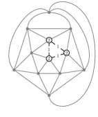
(a)

(b)

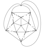
(c)

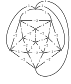
(d)

Figure 1: The diagrams illustrate certain vectors in $\mathbb{R}^{42}=\mathbb{R}^{|\mathcal{V}|}\times\mathbb{R}^{|\mathcal{E}|}$ thought of as vertex and edge labellings of the icosahedral graph. The labels specify the nonzero coordinates. Unlabeled vertices or edges (in gray) correspond to zero coordinates. Figure (a) is $(x_{C},y_{C})$ for a particular maximum clique in the icosahedral graph. Figures (b), (c), and (d) show certain vectors that are orthogonal to $(x_{C},y_{C})$ for all maximum cliques.

The $22$-dimensional orthogonal complement of the $20$-dimensional span of the $(x_{C},y_{C})$ has a basis given by the twelve vectors (one for each vertex) shown in Figure 1b, any five of the six vectors (one for each pair of antipodal vertices), shown in Figure 1c, and any five of the six vectors (one for each pair of antipodal vertices), shown in Figure 1d. Let $V$ be the $42\times 22$ matrix with these vectors as columns. One can check (e.g., by computing a rational LDL decomposition) that

$$V^{T}\begin{bmatrix}-11I_{12\times 12}&0\\ 0&4I_{30\times 30}\end{bmatrix}V\succeq 0.$$

If there were a correlation matrix with all of the $(x_{C},y_{C})$ in its nullspace, then it could be written in the form $VMV^{T}$ where $M\succeq 0$ and $[VMV^{T}]_{ii}=1$ for all $i=1,2,\ldots,42$. But then

$$-12=\textup{tr}\left(\begin{bmatrix}-11I_{12\times 12}&0\\ 0&4I_{30\times 30}\end{bmatrix}VMV^{T}\right)=\textup{tr}\left((V^{T}\begin{bmatrix}-11I_{12\times 12}&0\\ 0&4I_{30\times 30}\end{bmatrix}V)M\right),$$

and so $M$ cannot be positive semidefinite, and no such correlation matrix can exist. ∎

The following is an immediate corollary of Theorem 5.6 and Proposition 4.7. We state it explicitly because this appears to be the first known example of a cubic hyperbolic polynomial such that no power has a definite determinantal representation.

Corollary 5.7.

If $\mathcal{G}$ is the icosahedral graph, then no power of $p_{\mathcal{G},3}$, defined in (16), has a definite determinantal representation.

By using Proposition 4.13 together with our example of a hyperbolic, but not SOS-hyperbolic, cubic in $43$ variables (Theorem 5.6), we can construct such cubics whenever the number of variables is at least $43$.

Corollary 5.8.

If $n\geq 43$ and $e\in\mathbb{R}^{n}$, then $\mathcal{H}^{\textup{SOS}}_{n,3}(e)\subsetneq\mathcal{H}_{n,3}(e)$.

Although we have only been able to construct a hyperbolic cubic in $43$ variables that is not SOS-hyperbolic, it has been conjectured by Mario Kummer (personal communication), and seems likely, that such examples should already exist with five variables.

Conjecture 5.9.

If $n\geq 5$ and $e\in\mathbb{R}^{n}$, then $\mathcal{H}^{\textup{SOS}}_{n,3}(e)\subsetneq\mathcal{H}_{n,3}(e)$.

One way to resolve this conjecture, would be to find an explicit cubic form $q$ in four variables such that $\|x\|_{2}^{4}-2zq(x)+z^{2}\|x\|_{2}^{2}$ is nonnegative but is not a sum of squares. Then $p(x_{0},x)=x_{0}^{3}-3x_{0}\|x\|^{2}+2q(x)$ would be hyperbolic, but not SOS-hyperbolic, with respect to $e_{0}$.

6 Canonical linear functionals and the proof of Theorem 3.7

This section is devoted to developing tools used in the proof of Theorem 3.7 (and in Section 7 to follow), and then presenting the proof of Theorem 3.7 itself. We begin by showing how a hyperbolic polynomial $p\in\mathcal{H}_{n,d}(e)$, and a point $x\in\mathbb{R}^{n}$, define a set of linear functionals that generalize the orthogonal projectors onto the eigenspaces of a symmetric matrix. This construction may be of independent interest.

6.1 Canonical linear functionals

Given $p\in\mathcal{H}_{n,d}(e)$ and a fixed $x\in\mathbb{R}^{n}$, we define a collection of linear functionals associated with the eigenvalues of $x$. These are a generalization of the orthogonal projectors onto the eigenspaces of a symmetric matrix, as we shall see in Example 6.3. If $x$ has simple eigenvalues, these canonical linear functionals are the directional derivatives of the eigenvalues. If $u\in\mathbb{R}^{n}$, recall that

$$p(x+te+su)=p(e)\prod_{i=1}^{d}(t+t_{i}(s;x,u))$$

where the $t_{i}(s;x,u)$ are defined in Theorem 2.1. Let $x$ have eigenvalues $\lambda_{1}(x)>\ldots>\lambda_{k}(x)$ with multiplicities $m_{1},\ldots,m_{k}$. Let $I_{1},\ldots,I_{k}$ be a partition of $\{1,2,\ldots,d\}$ such that $|I_{i}|=m_{i}$ and $t_{j}(0;x,u)=\lambda_{i}(x)$ for all $j\in I_{i}$. Define the canonical linear functionals to be

$$\lambda_{i}^{\prime}(x)[u]:=\sum_{j\in I_{i}}t_{j}^{\prime}(0;x,u)\quad\textup{for $i=1,2,\ldots,k$}.$$

The following result summarizes the main properties of the $\lambda_{i}^{\prime}(x)[u]$ that we will need.

Lemma 6.1.

If $p\in\mathcal{H}_{n,d}(e)$ and $x\in\mathbb{R}^{n}$, then the maps $\mathbb{R}^{n}\ni u\mapsto\lambda_{i}^{\prime}(x)[u]$ satisfy:

1. $\displaystyle{\frac{D_{u}p_{x}(t)}{p_{x}(t)}=\sum_{i=1}^{k}\frac{\lambda_{i}^{\prime}(x)[u]}{\lambda_{i}(x)+t}}$;

2. $u\mapsto\lambda_{i}^{\prime}(x)[u]$ is linear;

3. $\lambda_{i}^{\prime}(x)[e]=m_{i}$, the multiplicity of the $i$th eigenvalue of $x$;

4. $\lambda_{i}^{\prime}(x)[x]=m_{i}\lambda_{i}(x)$;

5. $u\in\Lambda_{+}(p,e)$ if, and only if, $\lambda_{i}^{\prime}(x)[u]\geq 0$ for all $x\in\mathbb{R}^{n}$ and all $i$.

Proof.

The first statement follows from the following straightforward computation

$$\frac{D_{u}p_{x}(t)}{p_{x}(t)}=\frac{d}{ds}\left.\log(p(x+te+su))\right|_{s=0}=\sum_{j=1}^{d}\frac{t_{j}^{\prime}(0;x,u)}{t_{j}(0;x,u)+t}=\sum_{i=1}^{k}\frac{\lambda^{\prime}_{i}(x)[u]}{\lambda_{i}(x)+t}.$$

For the second statement, note that the numerator of $\frac{D_{u}p_{x}(t)}{p_{x}(t)}$ is linear in $u$, so the numerators, $\lambda_{i}^{\prime}(x)[u]$, of the partial fraction expansion in the first statement are also linear in $u$.

The third statement follows from the fact that $t_{j}(s;x,e)=\lambda_{i}(x)+s$ for all $i\in I_{i}$ so that $\lambda_{i}^{\prime}(x)[e]=|I_{i}|=m_{i}$. The fourth statement follows from the fact that $t_{j}(s;x,x)=\lambda_{i}(x)(1+s)$ for all $i\in I_{i}$ so that $\lambda^{\prime}_{i}(x)[x]=|I_{i}|\lambda_{i}(x)=m_{i}\lambda_{i}(x)$.

For the final statement, on the one hand, if $u\in\Lambda_{+}(p,e)$, then $t_{j}^{\prime}(0;x,u)\geq 0$ (by Theorem 2.1), and so $\lambda_{i}^{\prime}(x)[u]\geq 0$. On the other hand, if $\lambda^{\prime}_{i}(x)[u]\geq 0$ for all $x\in\mathbb{R}^{n}$ and all $i$, then $\frac{1}{m_{i}}\lambda^{\prime}_{i}(u)[u]=\lambda_{i}(u)\geq 0$ for all $i$, and so $u\in\Lambda_{+}(p,e)$. ∎

Remark 6.2.

We could have defined $\lambda_{i}^{\prime}(x)[u]$ via the first property in Lemma 6.1, as the residue of $D_{u}p_{x}(t)/p_{x}(t)$ corresponding to the simple pole at $-\lambda_{i}(x)$. Then we would need to show, directly, that these are nonnegative if, and only if, $u\in\Lambda_{+}(p,e)$, rather than relying on Theorem 2.1.

Example 6.3 (Canonical linear functionals for the determinant).

Let $p(X)=\det(X)$ where $X$ is a symmetric matrix and $e=I$. Suppose $X$ has $k$ distinct eigenvalues $\lambda_{1}(X),\ldots,\lambda_{k}(X)$ with corresponding multiplicities $m_{1},\ldots,m_{k}$. Then $X=\sum_{i=1}^{k}\lambda_{i}(X)P_{i}(X)$ where $P_{i}(X)$ is the orthogonal projector onto the eigenspace of $X$ corresponding to $\lambda_{i}(X)$. The associated canonical linear functionals are the maps $U\mapsto\textup{tr}(P_{i}(X)U)$. To see why, note that

$$\frac{D_{U}\det(X+tI)}{\det(X+tI)}=\textup{tr}(U(X+tI)^{-1})=\sum_{i=1}^{k}\frac{\textup{tr}(UP_{i}(X))}{t+\lambda_{i}(X)}.$$

These satisfy $\textup{tr}(P_{i}(X)I)=m_{i}$ and $\textup{tr}(P_{i}(X)X)=m_{i}\lambda_{i}(X)$ and $\textup{tr}(P_{i}(X)U)\geq 0$ for all $i$ and all $X$ if, and only if, $U\succeq 0$.

6.2 Proof of Theorem 3.7

By Proposition 3.4, it is enough to show that $u\in\Lambda_{+}(p,e)$ if, and only if, $H_{p,e}(x)[u]\succeq 0$ for all $x$. To achieve this, our main task is to express the parameterized Hermite matrix in terms of the canonical linear functionals.

Lemma 6.4.

Let $p\in\mathcal{H}_{n,d}(e)$ and $u\in\mathbb{R}^{n}$. With $y\in\mathbb{R}^{d}$ define a univariate polynomial $q_{y}(t)=y_{1}+y_{2}t+\cdots+y_{d}t^{d-1}$. Then, using the notation of Section 6.1, we have that

$$y^{T}H_{p,e}(x)[u]y=\sum_{i=1}^{k}[q_{y}(-\lambda_{i}(x))]^{2}\lambda_{i}^{\prime}(x)[u].$$

Proof.

We expand the rational function $t\mapsto\frac{D_{u}p_{x}(t)}{p_{x}(t)}$ as a Laurent series via

$$\frac{D_{u}p_{x}(t)}{p_{x}(t)}=\sum_{i=1}^{k}\frac{\lambda^{\prime}_{i}(x)[u]}{t+\lambda_{i}(x)}=\sum_{i=1}^{k}\lambda_{i}^{\prime}(x)[u]\sum_{\ell=1}^{\infty}(-\lambda_{i}(x))^{\ell-1}t^{-\ell}.$$

It then follows that $[H_{p,e}(x)[u]]_{j,\ell}=\sum_{i=1}^{k}\lambda_{i}^{\prime}(x)[u](-\lambda_{i}(x))^{j+\ell-2}$. The result follows because, for any $1\leq i\leq k$, $\sum_{j,\ell=1}^{d}y_{j}y_{\ell}(-\lambda_{i}(x))^{j+\ell-2}=[q_{y}(-\lambda_{i}(x))]^{2}$. ∎

Specialized to the determinant, this agrees with the explicit computation from Example 3.3.

Example 6.5 (Hankel matrix for the determinant).

Using the notation of Example 6.3, the quadratic form defined by the Hankel matrix is

$$y^{T}H_{p,e}(X)[U]y =\textstyle{\sum_{i=1}^{k}q_{y}(-\lambda_{i}(X))^{2}\textup{tr}(P_{i}(X)U)}$$

$$=\textstyle{\textup{tr}\left[\left(\sum_{i=1}^{k}q_{y}(-\lambda_{i}(X))^{2}P_{i}(X)\right)U\right]}=\textup{tr}((q_{y}(-X))^{2}U)$$

where $q_{y}(-X)=y_{1}+y_{2}(-X)+y_{3}(-X)^{2}+\cdots+y_{d}(-X)^{d-1}$.

We are now in a position to complete the proof of Theorem 3.7.

Corollary 6.6.

If $p\in\mathcal{H}_{n,d}(e)$, then $u\in\Lambda_{+}(p,e)$ if, and only if, $H_{p,e}(x)[u]\succeq 0$ for all $x$.

Proof.

If $u\in\Lambda_{+}(p,e)$, then $\lambda^{\prime}(x)[u]\geq 0$ for all $i$ and all $x$. From Lemma 6.4 it follows that $y^{T}H_{p,e}(x)[u]y\geq 0$ for all $x$ and all $y$. Conversely, suppose that $\lambda_{i}(u)<0$ for some $i$. Define $y$ so that the polynomial $q_{y}$ satisfies $q_{y}(-\lambda_{j}(x))=0$ if $j\neq i$ and $q_{y}(-\lambda_{j}(x))=1$ if $j=i$. Such a polynomial can be constructed via Lagrange interpolation, for instance. Then

$$y^{T}H_{p,e}(u)[u]y=\lambda_{i}^{\prime}(u)[u]=m_{i}\lambda_{i}(u)<0.$$

∎

7 View from the dual cone

In this section we consider the results obtained so far from the point of view of the dual cone

$$\Lambda_{+}(p,e)^{*}:=\{\xi\in(\mathbb{R}^{n})^{*}\;:\;\xi[x]\geq 0\;\;\textup{for all $x\in\Lambda_{+}(p,e)$}\},$$

the (closed convex) cone of linear functionals that take nonnegative values on $\Lambda_{+}(p,e)$. In particular, we study the image of the polynomial map $\phi_{p,e}=\phi^{H}_{p,e}$, defined in (7). We will see that this image contains the interior of the dual cone and is contained in the dual cone. Moreover, we give examples in which the image of $\phi_{p,e}$ is precisely the dual cone $\Lambda_{+}(p,e)^{*}$.

The image of $\phi_{p,e}$ can be expressed using the canonical linear functionals of Section 6.1.

Proposition 7.1.

If $p\in\mathcal{H}_{n,d}(e)$ and $x\in\mathbb{R}^{n}$ has $k\leq d$ distinct hyperbolic eigenvalues, then

$$\phi_{p,e}(x,\mathbb{R}^{d})=\textup{cone}\{\lambda_{1}^{\prime}(x)[\cdot],\ldots,\lambda_{k}^{\prime}(x)[\cdot]\}.$$

Proof.

From Lemma 6.4 we know that $\phi_{p,e}(x,y)=\sum_{i=1}^{k}(q_{y}(-\lambda_{i}(x)))^{2}\lambda^{\prime}_{i}(x)[\cdot]$ which is clearly a nonnegative combination of the linear functionals $\lambda_{i}^{\prime}(x)[\cdot]$. Conversely, given any nonnegative scalars $\eta_{1},\eta_{2},\ldots,\eta_{k}$, we can choose $y\in\mathbb{R}^{d}$ so that the polynomial $q_{y}$ (of degreee $d-1$) satisfies $q_{y}(-\lambda_{i}(x))=\sqrt{\eta_{i}}$ (by interpolation). This shows that any nonnegative combination of the $\lambda_{i}^{\prime}(x)[\cdot]$ is in the set $\phi_{p,e}(x,\mathbb{R}^{d})$. ∎

7.1 Parameterization of the dual cone up to closure

The following result shows that the map $\phi_{p,e}$ almost parameterizes the dual of the hyperbolicity cone. One inclusion follows directly from Theorem 3.7. The other direction follows, for instance, from the (well-known) fact that the gradient of $\log p(x)$ maps the interior of the hyperbolicity cone onto the relative interior of its dual cone. In the statement of the theorem we use the notation $\textup{int}(S)$ to denote the interior of the set $S$ and $\textup{relint}(S)$ to denote the relative interior.

Theorem 7.2.

If $p\in\mathcal{H}_{n,d}(e)$, then $\textup{relint}(\Lambda_{+}(p,e)^{*})\subseteq\phi_{p,e}(\mathbb{R}^{n},\mathbb{R}^{d})\subseteq\Lambda_{+}(p,e)^{*}$.

Proof.

The right hand inclusion follows from Theorem 3.7. Indeed if $u\in\Lambda_{+}(p,e)$, then

$$\phi_{p,e}(x,y)[u]\geq 0\quad\textup{for all $x\in\mathbb{R}^{n}$ and all $y\in\mathbb{R}^{d}$}$$

which implies that $\phi_{p,e}(\mathbb{R}^{n},\mathbb{R}^{d})\subseteq\Lambda_{+}(p,e)^{*}$. For the left-hand inclusion, let $\xi$ be an arbitrary linear functional in the relative interior of $\Lambda_{+}(p,e)^{*}$. Let $x$ be any optimal point (which exists because $\xi$ is in the relative interior of the dual cone) of the convex optimization problem

$$\min_{x\in\Lambda_{+}(p,e)}-\log p(x)\;\;\textup{subject to}\;\;\xi[x]=d.$$

Then $x\in\textup{int}(\Lambda_{+}(p,e))$ (because the objective function goes to infinity on the boundary) and so $\lambda_{i}(x)>0$ for all $i$. From the optimality conditions

$$\xi[u]=D_{u}\log p(x)=\sum_{i=1}^{k}\frac{\lambda_{i}^{\prime}(x)[u]}{\lambda_{i}(x)}\quad\textup{for all $u\in\mathbb{R}^{n}$.}$$

It follows that $\xi[\cdot]\in\textup{cone}\{\lambda_{1}^{\prime}(x)[\cdot],\ldots,\lambda_{k}^{\prime}(x)[\cdot]\}\subseteq\phi_{p,e}(x,\mathbb{R}^{d})$ (by Proposition 7.1). ∎

Remark 7.3.

If $p$ is a complete hyperbolic polynomial, the gradient of $\log p(x)$ gives a rational bijection between the interior of a hyperbolicity cone and the interior of its dual cone. A key difference between $\phi_{p,e}$ and the gradient of $\log p(x)$ is that the former maps all of $\mathbb{R}^{n}\times\mathbb{R}^{d}$ into the dual cone $\Lambda_{+}(p,e)^{*}$, where as the latter only maps the hyperbolicity cone itself into the dual cone. This difference allows us to construct polynomials that are globally nonnegative, rather than just nonnegative restricted to the open hyperbolicity cone.

We have seen that the image of $\phi_{p,e}$ is sandwiched between the interior of the dual cone and the dual cone itself. The following example shows that the image of $\phi_{p,e}$ may not contain all of the boundary of the dual cone.

Example 7.4 (Singular cubic curve).

Consider the hyperbolic cubic

$$p(x_{1},x_{2},x_{3})=\det\mathcal{A}(x)\quad\textup{where}\quad\mathcal{A}(x)=\begin{bmatrix}x_{3}&0&x_{1}\\ 0&x_{1}+x_{3}&x_{2}\\ x_{1}&x_{2}&x_{3}\end{bmatrix}$$

taken from [Hen10, Section 4.1]. From the definite determinantal representation we can see that $p$ is hyperbolic with respect to $e=(0,0,1)$. Its dual cone can be parameterized by

$$\Lambda_{+}(p,e)^{*}=\{\mathcal{A}^{*}(zz^{T})=(z_{2}^{2}+2z_{1}z_{3},2z_{2}z_{3},z_{1}^{2}+z_{2}^{2}+z_{3}^{2}):z\in\mathbb{R}^{3}\}$$

as discussed in [Hen10]. The intersection of the hyperbolicity cone with the affine hyperplane $\{x:\langle e,x\rangle=1\}$ and the intersection of $\phi_{p,e}(\mathbb{R}^{3},\mathbb{R}^{3})$ with the affine hyperplane $\{z:\langle e,z\rangle=1\}$ are shown in Figure 2.

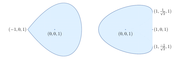
Figure 2: On the left is $\Lambda_{+}(p,e)\cap\{x:\langle e,x\rangle=1\}$, and on the right is $\phi_{p,e}(\mathbb{R}^{3},\mathbb{R}^{3})\cap\{z:\langle z,e\rangle=1\}$, where $p$ is the cubic from Example 7.4.

The intersection of $\Lambda_{+}(p,e)^{*}$ with the same affine hyperplane is the closure of the set shown on the right in Figure 2. The dual cone $\Lambda_{+}(p,e)^{*}$ and the image of $\phi_{p,e}$ differ in one has a two-dimensional face given by the conic hull of $(1,1/\sqrt{2},1)$ and $(1,-1/\sqrt{2},1)$, and in the other this face is replaced by the single ray generated by $(1,0,1)$.

7.2 Exact parameterizations of the dual cone

We now study certain situations in which the image of $\phi_{p,e}$ is precisely the closed dual cone. From Example 7.4, we know that this does not always occur. In this section we show that the image of $\phi_{p,e}$ is the closed dual cone $\Lambda_{+}(p,e)^{*}$ when, for instance, $p$ is strictly hyperbolic (see below for a definition), $p$ is a product of linear forms, or $p$ is the determinant restricted to symmetric matrices.

If $p\in\mathcal{H}_{n,d}(e)$ and $x\in\mathbb{R}^{n}$, we define the multiplicity of $x$ to be the multiplicity of the root $t=0$ of $p_{x}(t)$. If $p_{x}(0)\neq 0$, then we define the multiplicity of $x$ to be zero. A polynomial $p\in\mathcal{H}_{n,d}(e)$ is strictly hyperbolic if every element $x\in\mathbb{R}^{n}$ that is not a multiple of $e$ has $n$ distinct hyperbolic eigenvalues. It follows that if $p$ is strictly hyperbolic and $x$ is nonzero and satisfies $p(x)=0$, then $x$ has multiplicity $1$, the gradient of $p$ at $x$ is non-zero, and $x$ is a smooth point of the boundary of the hyperbolicity cone.

Proposition 7.5.

If $p\in\mathcal{H}_{n,d}(e)$ is strictly hyperbolic, then $\phi_{p,e}(\mathbb{R}^{n},\mathbb{R}^{d})=\Lambda_{+}(p,e)^{*}$.

Proof.

From Theorem 7.2 we know that $\Lambda_{+}(p,e)^{*}\supseteq\phi_{p,e}(\mathbb{R}^{n},\mathbb{R}^{d})\supseteq\textup{int}(\Lambda_{+}(p,e)^{*})$. It suffices to show that for any $\xi\in\partial\Lambda_{+}(p,e)^{*}$ there exists $x\in\mathbb{R}^{n}$ such that $\xi\in\phi_{p,e}(x,\mathbb{R}^{d})$.

Any non-zero $\xi\in\partial\Lambda_{+}(p,e)^{*}$ must vanish at some $x_{\xi}\in\partial\Lambda_{+}(p,e)\setminus\{0\}$ (since otherwise $\xi$ would be in the interior of the dual cone). Since $x_{\xi}$ is a non-zero element of the boundary of the hyperbolicity cone, it is a smooth point. As such, there is a unique supporting hyperplane to the cone at $x_{\xi}$. Since $x$ is in the boundary of the hyperbolicity cone, $\lambda_{\min}(x_{\xi})=0$ and so $\lambda_{\min}^{\prime}(x_{\xi})[x_{\xi}]=0$. Both $\xi$ and $\lambda_{\min}^{\prime}(x_{\xi})$ define supporting hyperplanes at $x_{\xi}$, so one must be a nonnegative multiple of the other. In particular $\xi$ is in the cone over the canonical linear functionals at $x_{\xi}$ and so is an element of the image of $\phi_{p,e}$. ∎

In the case where our hyperbolic polynomial is a product of distinct linear forms, so that the resulting hyperbolicity cone is polyhedral, the image of $\phi_{p,e}$ is the closed dual cone.

Proposition 7.6.

If $p\in\mathcal{H}_{n,d}(e)$ is a product of distinct linear forms, i.e., $p(x)=\prod_{i=1}^{d}a_{i}[x]$ with $a_{i}[e]>0$ for all $i$ and $a_{i}\neq a_{j}$ for all $i,j$, then $\phi_{p,e}(\mathbb{R}^{n},\mathbb{R}^{d})=\Lambda_{+}(p,e)^{*}$.

Proof.

Let $x$ be a generic point in $\mathbb{R}^{n}$, so that $x$ has $d$ distinct eigenvalues which are $\lambda_{i}(x)=a_{i}[x]/a_{i}[e]$ for $i=1,2,\ldots,d$. Since the eigenvalue functions are linear, the canonical linear functions are simply $\lambda_{i}^{\prime}(x)[u]=a_{i}[u]/a_{i}[e]$ for $i=1,2,\ldots,d$. From Proposition 7.1 we know that

$$\phi_{p,e}(x,\mathbb{R}^{d})=\textup{cone}\{\lambda_{1}^{\prime}(x),\ldots,\lambda_{d}^{\prime}(x)\}.$$

This is the cone generated by the linear forms $a_{1},\ldots,a_{d}$, which is just $\Lambda_{+}(p,e)^{*}$. ∎

Another case in which the image of $\phi_{p,e}$ is the dual cone is when $p$ is the determinant restricted to symmetric matrices.

Proposition 7.7.

Let $p(X)=\det(X)$ be the determinant restricted to $d\times d$ real symmetric matrices. Then $\phi_{p,I}(\mathcal{S}^{d},\mathbb{R}^{d})=\Lambda_{+}(p,I)^{*}$.

Proof.

Since the positive semidefinite cone is self-dual it follows that an arbitrary element of $\Lambda_{+}(p,I)^{*}$ has the form $U\mapsto\textup{tr}(ZU)$ where $Z\succeq 0$. Let $y=e_{2}=(0,1,0,\ldots,0)$ so that $q_{y}(t)=t$ in the notation of Example 6.5. Let $X=Z^{1/2}$ be the positive semidefinite square root of $Z$. If $U\in\mathcal{S}^{d}$, from Example 6.5 we have that

$$\phi_{p,I}(X,y)=\textup{tr}((-X)^{2}U)=\textup{tr}(X^{2}U)=\textup{tr}(ZU).$$

Since $Z$ was an arbitrary positive semidefinite matrix, we are done. ∎

8 Connections with interlacers

To conclude, we discuss the connection between our work and interlacing polynomials. If $p\in\mathcal{H}_{n,d}(e)$ and $q\in\mathcal{H}_{n,d-1}(e)$, we say that $q$ interlaces $p$ with respect to $e$ if the hyperbolic eigenvalues of any $x\in\mathbb{R}^{n}$ with respect to $p$ and $q$ satisfy

$$\lambda_{1}^{p}(x)\geq\lambda_{1}^{q}(x)\geq\lambda_{2}^{p}(x)\geq\cdots\geq\lambda_{d-1}^{q}(x)\geq\lambda_{d}^{p}(x).$$

For a fixed hyperbolic polynomial $p\in\mathcal{H}_{n,d}(e)$ the cone $\textup{Int}_{e}(p)$ of polynomials $q$ that interlace $p$ with respect to $e$ is a convex cone. In [KPV15, KNP18] it is shown that the cone of interlacers of $p\in\mathcal{H}_{n,d}(e)$ can be described by

$$\textup{Int}_{e}(p)=\{q\in\mathbb{R}[x]_{d-1}\;:\;B(p_{x},q_{x})\succeq 0\quad\textup{for all $x\in\mathbb{R}^{n}$}\}.$$

Much of the development of Sections 3 and 6 could have been presented from the point of view of interlacers. This is because $D_{u}p(x)\in\textup{Int}_{e}(p)$ if, and only if, $u\in\Lambda_{+}(p,e)$, so the hyperbolicity cone is a section of the cone of interlacers [KPV15].

The argument we used to show that every ternary hyperbolic polynomial is SOS-hyperbolic actually generalizes to give a projected spectrahedral description of the cone of interlacers of any ternary hyperbolic polynomial. This was first observed by Kummer, Naldi, and Plaumann [KNP18] via a seemingly quite different proof.

Proposition 8.1 ([KNP18, Page 17]).

If $p\in\mathcal{H}_{3,d}(e)$, then

$$\textup{Int}_{e}(p)=\{q\in\mathbb{R}[x_{1},x_{2},x_{3}]_{d-1}:B(p_{x},q_{x})\;\;\textup{is a matrix sum of squares}\}.$$

Proof.

Recall that $B(p_{x},q_{x})$ is a matrix sum of squares if, and only if, the restriction to a two-dimensional subspace not containing $e$ is a matrix sum of squares. But, after choosing appropriate coordinates, this is a matrix with entries that are each homogeneous forms in two variables, and so is a matrix sum of squares via [BSV16, Remark 5.10]. ∎

If $p$ is hyperbolic and has degree two, then the cone of interlacers of $p$ with respect to $e$ is simply the set of linear forms that are nonnegative on the cone $\Lambda_{+}(p,e)$. This is the dual cone, $\Lambda_{+}(p,e)^{*}$, which is again a quadratic cone, and so is a spectrahedron. Another case where we might expect the cone of interlacers to have a nice description is the case of hyperbolic polynomials of degree three in four variables.

Question 8.2.

If $p\in\mathcal{H}_{4,3}(e)$, is the cone of interlacers $\textup{Int}_{e}(p)$ a projected spectrahedron?

Acknowledgements

I would like to thank Amir Ali Ahmadi, Petter Brändén, Hamza Fawzi, Mario Kummer, Simone Naldi, Pablo Parrilo, Levent Tunçel, and Cynthia Vinzant for helpful discussions and correspondence related to various aspects of this work, and the anonymous referees for their thoughtful suggestions that have improved the article.

Appendix A Relating Bézoutians and Hankel matrices

In this appendix we prove Proposition 2.2. Before doing so, we establish a slightly simpler statement in which the dimension of the Bézoutian and Hankel matrices is the same as $\textup{deg}(a)$.

Proposition A.1.

If $a(t)=a_{0}+a_{1}t+\cdots+t^{d}$ is a monic polynomial of degree $d$ and $b$ is a polynomial of degree strictly less than $d$, then

$$B_{d}(a,b)=B(a,1)H_{d}\!\left(\frac{b}{a}\right)B(a,1)\quad\textup{where}\quad[B(a,1)]_{ij}=\begin{cases}a_{i+j-1}&\textup{if $1\leq i+j-1\leq d-1$}\\ 1&\textup{if $i+j-1=d$}\\ 0&\textup{otherwise}\end{cases}$$

is the (symmetric and unimodular) Bézoutian of $a$ and the constant polynomial $1$.

Proof.

This result is established in [BMO⁺11, Proposition 7.15]. We reproduce the proof here because there are some confusing typographic errors in [BMO⁺11, page 75]. The argument presented there uses the fact that the Hankel matrix $H_{d}\!\left(\frac{b}{a}\right)$ satisfies the identity

$$\frac{\frac{b(t)}{a(t)}-\frac{b(s)}{a(s)}}{s-t}=\sum_{p,q=1}^{\infty}h_{p+q-1}t^{-p}s^{-q}.$$

Combining this with the defining identity of the Bézoutian (5) we obtain

$$\sum_{i,j=1}^{d}[B(a,b)]_{ij}t^{i-1}s^{j-1}=a(t)\frac{\frac{b(t)}{a(t)}-\frac{b(s)}{a(s)}}{s-t}a(s)=\sum_{m,\ell=0}^{d}\sum_{p,q=1}^{\infty}a_{m}h_{p+q-1}a_{\ell}t^{m-p}s^{\ell-p}.$$

Changing variables via $i=m-p+1$ and $j=\ell-q+1$, and defining $a_{i}=0$ for $i>d$, gives

$$\sum_{i,j=1}^{d}[B(a,b)]_{ij}t^{i-1}s^{j-1}=\sum_{i,j=1}^{d}\left[\sum_{p,q=1}^{\infty}a_{i+p-1}h_{p+q-1}a_{j+q-a}\right]t^{i-1}s^{j-1}$$

from which the matrix identity follows.

The fact that $B(a,1)$ is unimodular follows directly from the fact that, if we reverse the order of the rows of $B(a,1)$ (which either preserves the determinant or changes its sign), we obtain a lower triangular matrix with unit diagonal. ∎

We now consider the case in which the dimension of the Bézoutian and Hankel matrices is possibly larger than the degree of the polynomial $a$.

Proof of Proposition 2.2.

Let $\tilde{a}(t)=t^{m-d}a(t)$ and $\tilde{b}(t)=t^{m-d}b(t)$. First note that

$$B_{m}(\tilde{a},\tilde{b})=\begin{bmatrix}0_{m-d,m-d}&0_{m-d,d}\\ 0_{d,m-d}&B_{d}(a,b)\end{bmatrix} \!=\!\begin{bmatrix}0_{m-d,d}&I_{m-d}\\ I_{d}&0_{d,m-d}\end{bmatrix}\!\!\begin{bmatrix}B_{d}(a,b)&0_{d,m-d}\\ 0_{m-d,d}&0_{m-d,m-d}\end{bmatrix}\!\!\begin{bmatrix}0_{m-d,d}&I_{m-d}\\ I_{d}&0_{d,m-d}\end{bmatrix}^{T}$$

$$\!=\!\begin{bmatrix}0_{m-d,d}&I_{m-d}\\ I_{d}&0_{d,m-d}\end{bmatrix}B_{m}(a,b)\begin{bmatrix}0_{m-d,d}&I_{m-d}\\ I_{d}&0_{d,m-d}\end{bmatrix}^{T}.$$

By Proposition A.1, and the fact that $\frac{\tilde{b}}{\tilde{a}}=\frac{b}{a}$, we see that

$$B(\tilde{a},1)H_{m}\!\left(\frac{\tilde{b}}{\tilde{a}}\right)B(\tilde{a},1) =B(\tilde{a},1)H_{m}\!\left(\frac{b}{a}\right)B(\tilde{a},1)$$

$$=B_{m}(\tilde{a},\tilde{b})=\begin{bmatrix}0_{d,m-d}&I_{d}\\ I_{m-d}&0_{m-d,d}\end{bmatrix}B_{m}(a,b)\begin{bmatrix}0_{d,m-d}&I_{d}\\ I_{m-d}&0_{m-d,d}\end{bmatrix}^{T}.$$

Since $B(\tilde{a},1)$ is symmetric and unimodular and has entries that are linear in the coefficients of $a$, we see that

$$M(a)=\begin{bmatrix}0_{d,m-d}&I_{d}\\ I_{m-d}&0_{m-d,d}\end{bmatrix}^{-1}B(\tilde{a},1)$$

is unimodular and has entries that are linear in the coefficients of $a$, completing the proof. ∎

References

- [AB18] N. Amini and P. Brändén. Non-representable hyperbolic matroids. Adv. Math., 334:417–449, 2018.
- [ABG70] M. F. Atiyah, R. Bott, and L. Gårding. Lacunas for hyperbolic differential operators with constant coefficients I. Acta Math., 124(1):109–189, 1970.
- [Ami19] N. Amini. Spectrahedrality of hyperbolicity cones of multivariate matching polynomials. J. Algebraic Combin., 50(2):165–190, 2019.
- [BK07] A. Buckley and T. Košir. Determinantal representations of smooth cubic surfaces. Geom. Dedicata, 125(1):115–140, 2007.
- [BM16] B. Barak and A. Moitra. Noisy tensor completion via the sum-of-squares hierarchy. In Conference on Learning Theory, pages 417–445, 2016.
- [BMO+11] D. A. Bini, V. Mehrmann, V. Olshevsky, E. Tyrtsyhnikov, and M. van Barel. Numerical Methods for Structured Matrices and Applications: The Georg Heinig Memorial Volume, volume 199. Springer Science & Business Media, 2011.
- [BPT12] G. Blekherman, P. A. Parrilo, and R. R. Thomas. Semidefinite optimization and convex algebraic geometry. SIAM, 2012.
- [Brä11] P. Brändén. Obstructions to determinantal representability. Adv. Math., 226(2):1202–1212, 2011.
- [Brä14] P. Brändén. Hyperbolicity cones of elementary symmetric polynomials are spectrahedral. Optim. Lett., 8(5):1773–1782, 2014.
- [BSV16] G. Blekherman, G. Smith, and M. Velasco. Sums of squares and varieties of minimal degree. J. Amer. Math. Soc., 29(3):893–913, 2016.
- [BVY14] S. Burton, C. Vinzant, and Y. Youm. A real stable extension of the Vámos matroid polynomial. arXiv preprint arXiv:1411.2038, 2014.
- [CP17] D. Cifuentes and P. A. Parrilo. Sampling algebraic varieties for sum of squares programs. SIAM J. Optim., 27(4):2381–2404, 2017.
- [DHO+16] J. Draisma, E. Horobeţ, G. Ottaviani, B. Sturmfels, and R. R. Thomas. The Euclidean distance degree of an algebraic variety. Found. Comput. Math., 16(1):99–149, 2016.
- [FWK05] J. Feldman, M. J. Wainwright, and D. R. Karger. Using linear programming to decode binary linear codes. IEEE Trans. Inform. Theory, 51(3):954–972, 2005.
- [Går59] L. Gårding. An inequality for hyperbolic polynomials. J. Math. Mech., pages 957–965, 1959.
- [GLPT12] J. Gouveia, M. Laurent, P. A. Parrilo, and R. Thomas. A new semidefinite programming hierarchy for cycles in binary matroids and cuts in graphs. Math. Program., 133(1-2):203–225, 2012.
- [Gül97] O. Güler. Hyperbolic polynomials and interior point methods for convex programming. Math. Oper. Res., 22(2):350–377, 1997.
- [Hen10] D. Henrion. Semidefinite geometry of the numerical range. Electron. J. Linear Algebra, 20(1):322–332, 2010.
- [HLJ13] F. R. Harvey and H. B. Lawson Jr. Gårding’s theory of hyperbolic polynomials. Comm. Pure Appl. Math., 66(7):1102–1128, 2013.
- [HV07] J. W. Helton and V. Vinnikov. Linear matrix inequality representation of sets. Comm. Pure Appl. Math., 60(5):654–674, 2007.
- [Kar72] R. M. Karp. Reducibility among combinatorial problems. In R. E. Miller and J. W. Thatcher, editors, Complexity of computer computations, pages 85–103. Springer, 1972.
- [KN81] M. G. Krein and M. A. Naimark. The method of symmetric and Hermitian forms in the theory of the separation of the roots of algebraic equations. Linear Multilinear Algebra, 10(4):265–308, 1981.
- [KNP18] M. Kummer, S. Naldi, and D. Plaumann. Spectrahedral representations of plane hyperbolic curves. arXiv preprint arXiv:1807.10901, 2018.
- [KPV15] M. Kummer, D. Plaumann, and C. Vinzant. Hyperbolic polynomials, interlacers, and sums of squares. Math. Program., 153(1):223–245, 2015.
- [Kum16] M. Kummer. A note on the hyperbolicity cone of the specialized Vámos polynomial. Acta Appl. Math., 144(1):11–15, 2016.
- [Las01] J. B. Lasserre. Global optimization with polynomials and the problem of moments. SIAM J. Optim., 11(3):796–817, 2001.
- [LPR05] A. S. Lewis, P. A. Parrilo, and M. Ramana. The Lax conjecture is true. Proc. Amer. Math. Soc., 133(9):2495–2499, 2005.
- [LRS15] J. R. Lee, P. Raghavendra, and D. Steurer. Lower bounds on the size of semidefinite programming relaxations. In Proc. 47th ACM Symposium on Theory of Computing, pages 567–576. ACM, 2015.
- [MS65] T. S. Motzkin and E. G. Straus. Maxima for graphs and a new proof of a theorem of Turán. Canad. J. Math., 17:533–540, 1965.
- [MSS15] A. Marcus, D. A. Spielman, and N. Srivastava. Finite free convolutions of polynomials. arXiv preprint arXiv:1504.00350, 2015.
- [MT14] T. Myklebust and L. Tunçel. Interior-point algorithms for convex optimization based on primal-dual metrics. arXiv preprint arXiv:1411.2129, 2014.
- [Nes00] Yu. Nesterov. Squared functional systems and optimization problems. In High performance optimization, pages 405–440. Springer, 2000.
- [Nes03] Yu. Nesterov. Random walk in a simplex and quadratic optimization over convex polytopes. Technical report, CORE Discussion Papers 2003/71, 2003.
- [NPT13] T. Netzer, D. Plaumann, and A. Thom. Determinantal representations and the Hermite matrix. Michigan Math. J., 62(2):407–420, 2013.
- [Par03] P. A. Parrilo. Semidefinite programming relaxations for semialgebraic problems. Math. Program., 96(2):293–320, 2003.
- [PP12] F. Permenter and P. A. Parrilo. Selecting a monomial basis for sums of squares programming over a quotient ring. In Proceedings 51st IEEE Conference on Decision and Control (CDC), pages 1871–1876. IEEE, 2012.
- [PV13] D. Plaumann and C. Vinzant. Determinantal representations of hyperbolic plane curves: an elementary approach. J. Symbolic Comput., 57:48–60, 2013.
- [RDL15] D. M. Rosen, C. DuHadway, and J. J. Leonard. A convex relaxation for approximate global optimization in simultaneous localization and mapping. In 2015 IEEE International Conference on Robotics and Automation (ICRA), pages 5822–5829. IEEE, 2015.
- [Ren06] J. Renegar. Hyperbolic programs, and their derivative relaxations. Found. Comput. Math., 6(1):59–79, 2006.
- [Ren16] J. Renegar. “Efficient” subgradient methods for general convex optimization. SIAM J. Optim., 26(4):2649–2676, 2016.
- [Ren19] J. Renegar. Accelerated first-order methods for hyperbolic programming. Math. Program., 173(1–2):1–35, 2019.
- [RS14] J. Renegar and M. Sondjaja. A polynomial-time affine-scaling method for semidefinite and hyperbolic programming. arXiv preprint arXiv:1410.6734, 2014.
- [Sau18] J. Saunderson. A spectrahedral representation of the first derivative relaxation of the positive semidefinite cone. Optim. Lett., 12(7):1475–1486, 2018.
- [Sch18] C. Scheiderer. Spectrahedral shadows. SIAM J. Appl. Algebra Geom., 2(1):26–44, 2018.
- [Sho87] N. Z. Shor. Class of global minimum bounds of polynomial functions. Cybernet. Systems Anal., 23(6):731–734, 1987.
- [SP15] J. Saunderson and P. A. Parrilo. Polynomial-sized semidefinite representations of derivative relaxations of spectrahedral cones. Math. Program., 153(2):309–331, 2015.