UTHEP-734

Diffeomorphisms on Fuzzy Sphere

Goro Ishiki^1),2) and Takaki Matsumoto^2),3)

¹⁾ Tomonaga Center for the History of the Universe, University of Tsukuba,
Tsukuba, Ibaraki 305-8571, Japan

²⁾ Graduate School of Pure and Applied Sciences, University of Tsukuba,
Tsukuba, Ibaraki 305-8571, Japan

³⁾ School of Theoretical Physics, Dublin Institute for Advanced Studies,
10 Burlington Road, Dublin 4, Ireland

Diffeomorphisms can be seen as automorphisms of the algebra of functions. In the matrix regularization, functions on a smooth compact manifold are mapped to finite size matrices. We consider how diffeomorphisms act on the configuration space of the matrices through the matrix regularization. For the case of the fuzzy $S^{2}$, we construct the matrix regularization in terms of the Berezin-Toeplitz quantization. By using this quantization map, we define diffeomorphisms on the space of matrices. We explicitly construct the matrix version of holomorphic diffeomorphisms on $S^{2}$. We also propose three methods of constructing approximate invariants on the fuzzy $S^{2}$. These invariants are exactly invariant under area-preserving diffeomorphisms and only approximately invariant (i.e. invariant in the large-$N$ limit) under the general diffeomorphisms.

Introduction

The matrix regularization [1, 2] gives a regularization of the world volume theory of membranes with the world volume $\mathbf{R}\times\Sigma$ where $\Sigma$ is a compact Riemann surface with a fixed topology. Although the original world volume theory has the world volume diffeomorphism symmetry, it is restricted to area-preserving diffeomorphisms on $\Sigma$ in the light-cone gauge. In this gauge fixing, we have a Poisson bracket defined by a volume form on $\Sigma$, which is invariant under the residual gauge transformations. The matrix regularization is an operation of replacing the Poisson algebra of functions on $\Sigma$ by the Lie algebra of $N\times N$ matrices. After this replacement, the world volume theory in the light-cone gauge becomes a quantum mechanical system with matrix variables. Remarkably enough, the regularized theory coincides with the BFSS matrix model which is conjectured to give a complete formulation of M-theory in the infinite momentum frame [3]. This coincidence suggests that the matrix regularization is not just a regularization of the world volume theory but a fundamental formulation of M-theory. The matrix regularization is also applied to type IIB string theory and provides a matrix model for a nonperturbative formulation of the string theory [4].

The regularized membrane theory has the $U(N)$ gauge symmetry which acts on the matrix variables as unitary similarity transformations. This symmetry should correspond to the are-preserving diffeomorphisms on $\Sigma$. However, we have not completely understood how general diffeomorphisms on $\Sigma$ act on the matrix variables. Since diffeomorphisms should be essential in constructing a covariant formulation of M-theory, it is important to clarify the full diffeomorphisms in the matrix model. The description of general diffeomorphisms in terms of matrices may also enable us to formulate theories of gravity on noncommutative spaces [6, 7, 8, 9] using the matrix regularization.

In this paper, we focus on automorphisms of $C^{\infty}(\Sigma)$ induced by diffeomorphisms on $\Sigma$ rather than diffeomorphisms themselves. This is reasonable since the group of diffeomorphisms on $\Sigma$ is isomorphic to automorphisms of $C^{\infty}(\Sigma)$. Under the matrix regularization, automorphisms of $C^{\infty}(\Sigma)$ are mapped to transformations between matrices. See Fig. 1. From this correspondence, we study how diffeomorphisms act on the space of the matrices.

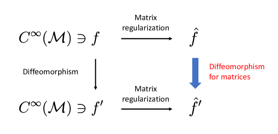
Figure 1: Under a diffeomorphism, a function $f$ is mapped to another function $f^{\prime}$. These functions are then mapped to matrices by the matrix regularization. By comparing the two matrices, we can read off how the diffeomorphism acts on the space of the matrices.

For this purpose, we need to fix the scheme of the matrix regularization. A systematic scheme is given by the Berezin-Toeplitz quantization [10, 11, 12], which is based on the concept of coherent states and has been developed in the context of the geometric and the deformation quantizations. In this paper, we construct the matrix regularization of $S^{2}$ in terms of the Berezin-Toeplitz quantization and investigate how diffeomorphisms on $S^{2}$, which are not necessarily are-preserving, act on the configuration space of the matrices. In particular, for holomorphic diffeomorphisms on $S^{2}$, we explicitly construct one-parameter deformations of the standard fuzzy $S^{2}$. We also propose three kinds of approximate diffeomorphism invariants on the fuzzy $S^{2}$. These are exactly invariant under area-preserving diffeomorphisms (the unitary similarity transformations) and also invariant under general diffeomorphisms in the large-$N$ limit.

The organization of this paper is as follows. In section 2, we introduce the basic terminology and notation concerning diffeomorphisms of a smooth manifold equipped with geometric structures. In section 3, we review the Berezin-Toeplitz quantization. In section 4, we define the action of diffeomorphisms on the space of matrices. In section 5, we construct the matrix regularization of $S^{2}$ based on the Berezin-Toeplitz quantization. Then, we investigate the holomorphic diffeomorphisms for matrices. In section 6, we propose the approximate invariants. In section 7, we summarize our results.

Diffeomorphisms and automorphisms

In this section, we review the notion of diffeomorphisms preserving geometric structures. See e.g. [19] for more details.

Let $M$ be a smooth compact manifold. We denote by $\text{Diff}(M)$ the group of diffeomorphisms from $M$ to itself. Let $\varphi\in\text{Diff}(M)$. For a smooth function $f$ on $M$, $\varphi$ induces a new function on $M$ defined by

$$f^{\prime}:=\varphi^{\ast}f=f\circ\varphi,$$ (2.1)

where $\varphi^{\ast}$ is the pullback by $\varphi$. The map $f\mapsto f^{\prime}$ defines an automorphism of $C^{\infty}(M)$. Inversely, an arbitrary automorphism of $C^{\infty}(M)$ is expressed in the form (2.1) using a diffeomorphism. This means that $\text{Diff}(M)$ is isomorphic to the group of automorphisms of $C^{\infty}(M)$ . More generally, for a tensor field $T$ on $M$, $\varphi$ induces a new tensor field $T^{\prime}$ on $M$ as the pullback or the pushforward. The map $T\mapsto T^{\prime}$ does not change the type of $T$ but generally changes the components of $T$. If $T=T^{\prime}$, then we say that $\varphi$ preserves $T$.

Let $\{\varphi_{t}\}_{t\in\mathbf{R}}$ be a one parameter group of diffeomorphisms, that is, the map from $\mathbf{R}\times M$ to $M$ defined by $(t,p)\mapsto\varphi_{t}(p)$ is smooth, $\varphi_{t}\circ\varphi_{s}=\varphi_{t+s}$ for any $t,s\in\mathbf{R}$ and $\varphi_{0}=\text{id}_{M}$. Since $\{\varphi_{t}\}_{t\in\mathbf{R}}$ gives a smooth curve $t\mapsto\varphi_{t}(p)$ on $M$, we can define the velocity vector field $u$ by

$$(uf)(p)=\evaluated{\frac{d}{dt}f(\varphi_{t}(p))}_{t=0}.$$ (2.2)

The infinitesimal transformation of $T$ induced by $\varphi_{t}$ is

$$\delta T:=\lim_{t\to 0}\frac{1}{t}(T^{\prime}-T)=L_{u}T,$$ (2.3)

where $L_{u}$ is the Lie derivative along $u$. If and only if $L_{u}T=0$, $\varphi_{t}$ preserves $T$ for any $t$.

We suppose that $T$ is a geometric structure on $M$, that is, $T$ has some special properties. For example, a Riemannian structure $g$ is a positive definite symmetric tensor field of type $(0,2)$, a symplectic structure $\omega$ is a non-degenerate, closed antisymmetric tensor field of type $(0,2)$, and a complex structure $J$ is a tensor field of type $(1,1)$ satisfying $J\circ J=-\text{id}_{M}$ and the integrability condition. If $\varphi$ preserves $T$, then $\varphi$ is called an automorphism of $(M,T)$. The subgroup of $\text{Diff}(M)$ consisting of all automorphisms of $(M,T)$ is called the automorphism group of $(M,T)$ and denoted by $\text{Aut}(M,T)$. Similarly, if $\varphi$ preserves several structures $T,T^{\prime},\ldots$, the corresponding automorphism group is denoted by $\text{Aut}(M,T,T^{\prime},\ldots)$.

The automorphism groups $\text{Aut}(M,g)$, $\text{Aut}(M,\omega)$ and $\text{Aut}(M,J)$ are also known as the groups of isometries, symplectomorphisms and holomorphic diffeomorphisms, respectively. Automorphism groups are often isomorphic to a finite dimensional Lie group depending on $T$ although $\text{Diff}(M)$ is an infinite dimensional Lie group. For example, any isometry group is known to be isomorphic to a finite dimensional Lie group.

For symplectic manifolds $(M,\omega)$ with the trivial first cohomology class, any vector field (2.2) generated by a symplectomorphism is a Hamiltonian vector field $u_{\alpha}$, which satisfies $d\alpha=\omega(u_{\alpha},\,\cdot\,)$ with a function $\alpha$ on $M$. Inversely, for any function $\alpha$, there is a unique Hamiltonian vector field $u_{\alpha}$. Hence, the generators of symplectomorphisms are labelled by functions on $M$. The infinitesimal transformation of a function $f$ induced by a symplectomorphism can be written as

$$\delta f=\omega(u_{f},u_{\alpha})=\{f,\alpha\},$$ (2.4)

where $\{\,\cdot\,,\,\cdot\,\}$ is the Poisson bracket. Since Hamiltonian vector fields satisfy $[u_{\alpha},u_{\beta}]=u_{\{\alpha,\beta\}}$, the Lie algebra of $\text{Aut}(M,\omega)$ is isomorphic to the Poisson algebra on $M$, which is an infinite dimensional Lie algebra.

Matrix regularization and Berezin-Toeplitz quantization

In this section, we review the construction of the matrix regularization based on the Berezin-Toeplitz quantization. In the following, we denote by $\{\,\cdot\,,\,\cdot\,\}$ the poisson bracket induced by the symplectic form $\omega$. We assume $(M,\omega)$ to be a $2n$-dimensional closed symplectic manifold.

Let $N_{1},N_{2},\ldots$ be a strictly monotonically increasing sequence of positive integers. The matrix regularization is formally defined by a family of linear maps from functions on $(M,\omega)$ to $N_{p}\times N_{p}$ matrices, $\{T_{p}:C^{\infty}(M)\rightarrow M_{N_{p}}(\mathbf{C})\}_{p\in\mathbf{N}}$, which satisfy

$$\begin{split}&\lim_{p\to\infty}\|T_{p}(f)T_{p}(g)-T_{p}(fg)\|=0,\\ &\lim_{p\to\infty}\|p[T_{p}(f),T_{p}(g)]-\mathrm{i}T_{p}(\{f,g\})\|=0,\end{split}$$ (3.1)

for any $f,g\in C^{\infty}(\Sigma)$ [21]. Here, $\|\cdot\|$ denotes an arbitrary matrix norm. In order to avoid the trivial case with $T_{p}(f)=0$, one may also assume for example that $\lim_{p\to\infty}\Tr T_{p}(f)=\int_{M}\omega^{n}f/n!$.

The conditions (LABEL:MR) and the linearity of $T_{p}$ means that $T_{p}$ is approximately a representation of the Poisson algebra on $\mathbf{C}^{N_{p}}$. Note that the matrix algebra is noncommutative and hence is never homomorphic to the commutative algebra of functions. The matrix regularization gives only an approximate homomorphism and the accuracy of the approximation improves as the matrix size tends to infinity.

The matrix regularization is closely related to the quantization of classical mechanics. Recall that, in the quantization, classical observables ${\cal O}(q,p)$, which are functions on the phase space, are promoted to quantum operators $\hat{\cal O}(\hat{q},\hat{p})$ and the classical Poisson bracket is replaced with the commutator of the operators. This relation is very similar to (LABEL:MR), where the large-$p$ limit in (LABEL:MR) corresponds to the classical limit $\hbar\rightarrow 0$. However, there is a crucial difference. The Hilbert space for quantum mechanics is infinite dimensional, while that of the matrix regularization is finite dimensional. This difference comes from the noncompactness of the classical phase space (i.e. one needs infinitely many wave packets to cover the entire noncompact phase space. This would not be the case if the phase space were compact.). In the matrix regularization, we always assume that the manifold $M$ is compact, so that the associated Hilbert space is finite dimensional. Hence, the matrix regularization is said to be the quantization on a compact phase space.

The quantization of classical mechanics is essentially given by fixing the ordering of the operators. For the anti-normal ordering, the quantization can be elegantly reformulated as the Berezin-Toeplitz quantization, which has been developed in the context of the geometric and the deformation quantizations [10, 11, 12]. See appendix A for the Berezin-Toeplitz quantization for quantum mechanics. The Berezin-Toeplitz quantization has a great advantage that it can be applied not only to the flat space but also to a large class of manifolds with $\text{spin}^{c}$ structures, giving a systematic way of generating the matrix regularizations for compact $\text{spin}^{c}$ manifolds.

Let us review the Berezin-Toeplitz quantization for $(M,\omega)$. Our setup is as follows. We choose a Riemannian metric $g$ and an almost complex structure $J$ such that they are compatible with $\omega$. Then, $M$ has a $\text{spin}^{c}$ structure associated with $J$. For the moment, we assume that this gives a spin structure. The case of general $\text{spin}^{c}$ manifolds will be mentioned in the last part of this section. Let $S$ be a spinor bundle over $M$. The fiber of $S$ is a spinor space $W\cong\mathbf{C}^{2^{n}}$, and spinor fields on $M$ are sections of $S$. Let $P$ be a principle $U(1)$-bundle over $M$ with a gauge connection $A$ and the curvature two-form $F=dA$. We consider the case with $F=2\pi\omega V_{n}^{-1/n}$, where $V_{n}=\int_{M}\omega^{n}/n!$ is the symplectic volume, so that $A$ is proportional to the symplectic potential. Let $L_{p}$ be an associated complex line bundle to $P$ for the irreducible representation $\pi_{p}:U(1)\to GL(1,\mathbf{C})$ defined by $\pi_{p}(e^{\mathrm{i}\theta})=e^{\mathrm{i}p\theta}$ ($\theta\in\mathbf{R}$, $p\in\mathbf{N}$). We consider a twisted spinor bundle $S\otimes L_{p}\simeq S\otimes L^{\otimes p}_{1}$ over $M$, where $L^{\otimes p}_{1}$ stands for the $p$-fold tensor product of $L_{1}$. The sections of this bundle are spinor fields on $M$ which take values in the representation space of $\pi_{p}$. We denote by $\Gamma(S\otimes L_{p})$ the vector space of the spinor fields and define a inner product by

$$(\psi,\phi)=\frac{1}{n!}\int_{M}\omega^{n}\,\psi^{\dagger}\cdot\phi,$$ (3.2)

for $\psi,\phi\in\Gamma(S\otimes L_{p})$, where $\psi^{\dagger}\cdot\phi$ denotes the Hermitian inner product on $W$ (i.e. the contraction of the spinor indices).

Then, we define the Dirac operator on $\Gamma(S\otimes L_{p})$. Let $U\subset M$ be an open subset and $\sigma^{\mu}$ $(\mu=1,2,\ldots,2n)$ local coordinates on $U$. We denote by $e_{a}$ $(a=1,2,\ldots,2n)$ an orthonormal frame on $U$ with respect to $g$ and by $\theta^{a}$ the dual basis of $e_{a}$. In the following, we raise and lower the indices of the orthonormal frame by using the Kronecker delta. Now we define a linear map $\gamma$ from vector fields on $U$ to endomorphisms of $W$ by

$$\gamma(e_{a})=\gamma_{a},$$ (3.3)

where $\gamma_{a}$ are the gamma matrices satisfying $\{\gamma_{a},\gamma_{b}\}=2\delta_{ab}\textbf{1}_{2^{n}}$. Using $\gamma_{a}$, we define the spin connection $\Omega^{ab}\gamma_{a}\gamma_{b}/4$, where $\Omega_{ab}$ is a local one-form determined by

$$\begin{split}&\Omega_{ab}+\Omega_{ba}=0,\\ &\Omega^{a}{}_{b}\wedge\theta^{b}+d\theta^{a}=0.\end{split}$$ (3.4)

Given these data, we define the Dirac operator on $\Gamma(S\otimes L_{p})$ by

$$D=\mathrm{i}\gamma(\partial^{\mu})\biggl{(}\partial_{\mu}+\frac{1}{4}\Omega^{ab}_{\mu}\gamma_{a}\gamma_{b}-\mathrm{i}pA_{\mu}\biggr{)},$$ (3.5)

where $\partial_{\mu}={\partial}/{\partial\sigma^{\mu}}$.

Finally, we construct the quantization map satisfying (LABEL:MR). Let $\psi_{i}$ $(i=1,2,\ldots,N_{p})$, be the orthonormal basis of $\text{Ker}D$ with respect to the inner product (3.2), where $N_{p}=\text{dim}\text{Ker}D$. At least for large $p$, the sequence $N_{p},N_{p+1},\ldots$ is in fact strictly monotonically increasing, as shown in appendix B. We define the so-called Toeplitz operator by

$$\matrixelement*{i}{T_{p}(f)}{j}=(\psi_{j},f\psi_{i}),$$ (3.6)

for $f\in C^{\infty}(M)$, where $\{\ket*{i}\mid i=1,2,\cdots,N_{p}\}$ is an orthonormal basis of $\textbf{C}^{N_{p}}$ corresponding to $\psi_{i}$. This is a generalization of (A.4). In this construction, the map $T_{p}(f)$ indeed satisfies the conditions (LABEL:MR) because of the asymptotic expansion [12],

$$T_{p}(f)T_{p}(g)=T_{p}(C_{0}(f,g))+\frac{1}{p}T_{p}(C_{1}(f,g))+O(p^{-2})$$ (3.7)

for any $f,g\in C^{\infty}(M)$, where $C_{0}(f,g)=fg$ and $C_{1}(f,g)-C_{1}(g,f)=\mathrm{i}\{f,g\}$.

So far, we have assumed that $M$ has a spin structure. However, the similar construction is also available for general $\text{spin}^{c}$ manifolds. In this case, an additional $U(1)$ connection is needed in the definition of the Dirac operator (3.5).

Matrix diffeomorphisms

In this section, we define the action of diffeomorphisms in the configuration space of matrices using the Toeplitz operator.

Let $(M,\omega)$ be a closed symplectic manifold. For $f\in C^{\infty}(M)$, we consider an automorphism $f\mapsto\varphi^{\ast}f$ induced by $\varphi\in\text{Diff}\,(M)$. By following the procedure in Fig. 1, we define a transformation of $N_{p}\times N_{p}$ matrices by

$$T_{p}(f)\mapsto T_{p}(\varphi^{\ast}f).$$ (4.1)

We call this transformation a matrix diffeomorphism corresponding to $\varphi$.

It is well-known that area-preserving diffeomorphisms (2.4) are realized as unitary similarity transformations in the matrix regularization. This can also be seen by comparing the symmetries of the light-cone membrane and the matrix model. The definition (4.1) also realizes this correspondence. From (3.7), one can see that the transformation (2.4) is mapped to the infinitesimal matrix diffeomorphism,

$$\delta T_{p}(f)=T_{p}(\delta f)=-\mathrm{i}p[T_{p}(f),T_{p}(\alpha)]+O(p^{-1}).$$ (4.2)

This is nothing but the infinitesimal form of a unitary similarity transformation.

Conversely, if (4.2) holds, then $\delta f$ is an area-preserving diffeomorphism. This is shown as follows. Suppose that (4.2) holds for a certain $\alpha\in C^{\infty}(M)$. Then, because of (LABEL:MR), we have $T_{p}(\delta f-\{\alpha,f\})=O(p^{-1})$. This is satisfied if and only if $\delta f-\{\alpha,f\}=0$ [21]. Hence, $\delta f$ is area-preserving. These arguments show that for non-area-preserving diffeomorphisms, the corresponding matrix diffeomorphisms cannot be written in the form (4.2).

Recall that diffeomorphisms can be regarded as automorphisms on the space of functions. On the other hand, matrix diffeomorphisms are not necessarily an automorphism of $M_{N_{p}}(\textbf{C})$, which can always be written as a similarity transformation. This is because the Toeplitz operator is not an isomorphism from $C^{\infty}(M)$ to $M_{N_{p}}(\textbf{C})$. In fact, the definition (4.1) contains a much broader class of transformations than the similarity transformations. In the next section, we will explicitly construct some of those transformations for fuzzy $S^{2}$.

Matrix diffeomorphisms on fuzzy sphere

In this section, we consider the Berezin-Toeplitz quantization and matrix diffeomorphisms on the fuzzy $S^{2}$ [24]. We will explicitly construct holomorphic matrix diffeomorphisms on the fuzzy $S^{2}$ and see that most of these transformations can not be written as a similarity transformation.

Berezin-Toeplitz quantization on $S^{2}$

We first construct the Berezin-Toeplitz quantization map for $S^{2}$. See appendix C for our notation and geometric structures on $S^{2}$, which we use below.

In the Berezin-Toeplitz quantization, we need spinors, which are sections of $S\otimes L_{p}$. Here, we take the Wu-Yang monopole configuration (C.10) as a connection of the line bundle $L_{1}$ and $S$ is the bundle of two-component spinors. The Dirac operator (3.5) on $\Gamma(S\otimes L_{p})$ can be decomposed as (B.1). The local form of $D^{\pm}$ on $U_{z}$ are given as

$$\begin{split}D^{+}&=\sqrt{2}\mathrm{i}\left\{(1+|z|^{2})\partial_{\bar{z}}+\frac{p-1}{2}z\right\},\\ D^{-}&=\sqrt{2}\mathrm{i}\left\{(1+|z|^{2})\partial_{z}-\frac{p+1}{2}\bar{z}\right\}.\end{split}$$ (5.1)

Here, we have used the geometric structures shown in appendix C.

In order to construct Toeplitz operators, we need the zero modes of $D^{\pm}$. We can easily solve the eigenvalue equations $D^{\pm}\psi^{\pm}=0$ and obtain $\psi^{+}=(1+|z|^{2})^{-(p-1)/2}h^{+}$ and $\psi^{-}=(1+|z|^{2})^{(p+1)/2}h^{-}$, where $h^{+}$ and $h^{-}$ are arbitrary holomorphic and anti-holomorphic functions on $U_{z}$, respectively. Note that the integral,

$$\int_{S^{2}}\omega\,|\psi^{-}|^{2}=\mathrm{i}\int_{S^{2}}dzd\bar{z}\,(1+|z|^{2})^{(p-1)}|h^{-}|^{2},$$ (5.2)

does not converge for $p\geq 1$, unless $h^{-}=0$. Thus, we find that $\text{Ker}D^{-}=\{0\}$ for $p\geq 1$. The similar integral for $\psi^{+}$ converges when the degree of $h^{+}$ is smaller than $p$. Such $h^{+}$ is a holomorphic polynomial of degree $p-1$, which can be expanded in terms of the basis $1,z,z^{2},\ldots,z^{p-1}$. Therefore, we find that $N_{p}=\text{dim}\text{Ker}D^{+}=p$. The Dirac zero modes can be written as

$$\psi_{i}(z,\bar{z})=\sqrt{\frac{p}{2\pi}}\left(\begin{array}[]{c}\innerproduct*{i}{z}\\ 0\end{array}\right),$$ (5.3)

where $\{\ket*{i}\mid i=1,2,\cdots,p\}$ is an arbitrary orthonormal basis of $\textbf{C}^{p}$, and $\ket{z}$ is the Bloch coherent state with $J=(p-1)/2$ defined by

$$\ket*{z}=\frac{1}{(1+|z|^{2})^{J}}\sum^{J}_{r=-J}z^{J-r}{\binom{2J}{J+r}}^{1/2}\ket*{Jr}.$$ (5.4)

Here, $\{\ket*{Jr}\mid r=-J,-J+1,\ldots,J\}$ is the standard basis of the $(2J+1)$-dimensional irreducible representation space of $SU(2)$. By using the resolution of identity, $p\int_{S^{2}}\omega\outerproduct*{z}{z}/2\pi=\textbf{1}_{p}$, one can check that $\{\psi_{i}\mid i=1,2,\cdots,p\}$ is an orthonormal basis of $\text{Ker}D$.

In the above setup, the Toeplitz operators (3.6) are written as

$$\matrixelement*{i}{T_{p}(f)}{j}=\frac{p}{2\pi}\int_{S^{2}}\omega\innerproduct*{i}{z}f(z,\bar{z})\innerproduct*{z}{i}.$$ (5.5)

Let us focus on the embedding coordinates $x^{A}$ from $S^{2}$ to $\textbf{R}^{3}$, which are smooth real valued functions on $S^{2}$. From (C.1), we have

$$\begin{split}x^{1}&=\frac{z+\bar{z}}{1+|z|^{2}},\\ x^{2}&=\frac{\mathrm{i}(\bar{z}-z)}{1+|z|^{2}},\\ x^{3}&=\frac{1-|z|^{2}}{1+|z|^{2}}.\end{split}$$ (5.6)

It is easy to find that the Toeplitz operators of $x^{A}$ are given by

$$T_{p}(x^{A})=\frac{L^{A}}{J+1},$$ (5.7)

where $L^{A}$ are the $p$-dimensional irreducible representation of the generators of $SU(2)$. This is the well-known configuration of the fuzzy $S^{2}$.

Holomorphic matrix diffeomorphisms

Here, we consider the matrix diffeomorphisms (4.1) for $X^{A}:=T_{p}(x^{A})$. Since there are infinitely many diffeomorphisms even for the simple manifold $S^{2}$, we restrict ourselves to the holomorphic diffeomorphisms $\varphi\in\text{Aut}\,(S^{2},J)$ in the following. See appendix D for a review of some automorphisms on $S^{2}$.

As reviewed in appendix D, any $\varphi\in\text{Aut}\,(S^{2},J)$ is expressed as a M$\ddot{\text{o}}$bius transformation (D.3). We focus on the four special transformations,

$$\begin{split}R_{\theta}(z)&=e^{\mathrm{i}\theta}z,\\ D_{\lambda}(z)&=e^{\lambda}z,\\ T_{\eta}(z)&=z+\eta,\\ S_{\zeta}(z)&=\frac{z}{\zeta z+1},\end{split}$$ (5.8)

where $\theta,\lambda\in\mathbf{R}$ and $\eta,\zeta\in\mathbf{C}$. These are a rotation, a dilatation, a translation and a special conformal transformation, respectively. Note that any M$\ddot{\text{o}}$bius transformation can be constructed as their composition. Note also that $R_{\theta}$ is an automorphism of $(S^{2},\omega,J,g)$ satisfying the condition (D.8), while the other three transformations are not. We consider one-parameter groups, $\{R_{t\theta}\}_{t\in\textbf{R}}$, $\{D_{t\lambda}\}_{t\in\textbf{R}}$, $\{T_{t\eta}\}_{t\in\textbf{R}}$ and $\{S_{t\zeta}\}_{t\in\textbf{R}}$, which generate the vector fields defined by (2.2),

$$\begin{split}u_{R}&=\mathrm{i}\theta(z\partial_{z}-\bar{z}\partial_{\bar{z}}),\\ u_{D}&=\lambda(z\partial_{z}+\bar{z}\partial_{\bar{z}}),\\ u_{T}&=\eta\partial_{z}+\bar{\eta}\partial_{\bar{z}},\\ u_{S}&=-\zeta z^{2}\partial_{z}-\bar{\zeta}\bar{z}^{2}\partial_{\bar{z}},\end{split}$$ (5.9)

respectively.

For a diffeomorphism generated by a vector field $u$, the infinitesimal variation of the embedding function $x^{A}$ is given as the Lie derivative $L_{u}x^{A}$, as reviewed in section 2. Correspondingly, the variation of the matrices are given by $\delta X^{A}=T_{p}(L_{u}x^{A})$. Let $X^{\pm}=T_{p}(x^{\pm})=T_{p}(x^{1}\pm\mathrm{i}x^{2})$. After some calculations, we easily find that the infinitesimal variations of $X^{A}$ for the vector fields (5.9) are given by

$$\begin{split}&\delta_{R}X^{+}=i\theta X^{+},\\ &\delta_{R}X^{-}=-i\theta X^{-},\\ &\delta_{R}X^{3}=0,\\ \end{split}$$ (5.10)

$$\begin{split}&\delta_{D}X^{+}=\lambda X^{3}X^{+}+O(p^{-1}),\\ &\delta_{D}X^{-}=\lambda X^{3}X^{-}+O(p^{-1}),\\ &\delta_{D}X^{3}=-\lambda X^{+}X^{-}+O(p^{-1}),\\ \end{split}$$ (5.11)

$$\begin{split}&\delta_{T}X^{+}=\frac{1}{2}\eta(\textbf{1}_{p}+X^{3})^{2}-\frac{1}{2}\bar{\eta}(X^{+})^{2}+O(p^{-1}),\\ &\delta_{T}X^{-}=\frac{1}{2}\bar{\eta}(\textbf{1}_{p}+X^{3})^{2}-\frac{1}{2}\eta(X^{-})^{2}+O(p^{-1}),\\ &\delta_{T}X^{3}=-\frac{1}{2}(\textbf{1}_{p}+X^{3})(\bar{\eta}X^{+}+\eta X^{-})+O(p^{-1}),\\ \end{split}$$ (5.12)

$$\begin{split}&\delta_{S}X^{+}=\frac{1}{2}\bar{\zeta}(\textbf{1}_{p}-X^{3})^{2}-\frac{1}{2}\zeta(X^{+})^{2}+O(p^{-1}),\\ &\delta_{S}X^{-}=\frac{1}{2}\zeta(\textbf{1}_{p}-X^{3})^{2}-\frac{1}{2}\bar{\zeta}(X^{-})^{2}+O(p^{-1}),\\ &\delta_{S}X^{3}=\frac{1}{2}(\textbf{1}_{p}-X^{3})(\zeta X^{+}+\bar{\zeta}X^{-})+O(p^{-1}).\end{split}$$ (5.13)

The rotation (LABEL:delta_R) can be written as $\delta_{R}X^{A}=-\mathrm{i}p[X^{A},\theta X^{3}/2]+O(p^{-1})$. This is the infinitesimal transformation of a unitary similarity transformation. More generally, we show in appendix E that any matrix diffeomorphism corresponding to $\varphi\in\text{Aut}(S^{2},\omega,J,g)$ is given by a unitary similarity transformation.

We also notice that the other three matrix diffeomorphisms are not unitary similarity transformations. For example, let us check the case of $\delta_{D}X^{A}$. If $\delta_{D}X^{3}$ is a similarity transformation, we have $\delta_{D}X^{3}\propto[U,X^{3}]$ with $U$ a certain matrix. Then, we will have

$$\expectationvalue*{\delta_{D}X^{3}}{Jr}=0,$$ (5.14)

for all $r$. However, $\expectationvalue*{\delta_{D}X^{3}}{Jr}=-\lambda(J+r)(J-r+1)/(J+1)^{2}$ is not zero for $r\neq-J$. Thus, the matrix diffeomorphism corresponding to $D_{t\lambda}$ is not a similarity transformation.

Our definition of the matrix diffeomorphisms also works for finite transformations. As an example, let us consider the dilatation. The finite diffeomorphism transforms of (5.6) are given by

$$\begin{split}D^{\ast}_{t\lambda}x^{1}&=\frac{e^{t\lambda}(z+\bar{z})}{1+e^{2t\lambda}|z|^{2}},\\ D^{\ast}_{t\lambda}x^{2}&=\frac{ie^{t\lambda}(\bar{z}-z)}{1+e^{2t\lambda}|z|^{2}},\\ D^{\ast}_{t\lambda}x^{3}&=\frac{1-e^{2t\lambda}|z|^{2}}{1+e^{2t\lambda}|z|^{2}}.\end{split}$$ (5.15)

In the following, we set $\lambda=1$ and $t\geq 0$ for simplicity. For example, the matrix elements $\matrixelement*{Jr}{T_{p}(D^{\ast}_{t}x^{3})}{Jr^{\prime}}$ reduces to the following integral,

$$\begin{split}I:=\int_{S^{2}}\omega\,\frac{z^{J-r}\bar{z}^{J-r^{\prime}}}{(1+|z|^{2})^{2J}}\frac{1-e^{2t}|z|^{2}}{1+e^{2t}|z|^{2}}.\\ \end{split}$$ (5.16)

After integrating out the argument of $z$ and exchanging the integral variable from $|z|^{2}$ to $y=1/(1+|z|^{2})$, we obtain

$$\begin{split}I&=2\pi\delta_{rr^{\prime}}(1+e^{-2t})\int^{1}_{0}dy\,y^{J+r+1}(1-y)^{J-r}\{1-(1-e^{-2t})y\}^{-1}\\ &\qquad-2\pi\delta_{rr^{\prime}}\int^{1}_{0}dy\,y^{J+r}(1-y)^{J-r}\{1-(1-e^{-2t})y\}^{-1}.\end{split}$$ (5.17)

For a while, we suppose that $t\neq 0$. For $t>0$, we have $|1-e^{-2t}|<1$. Using the integral representation of Gauss’s hyper geometric function $F(\alpha,\beta,\gamma;s)$ for $|s|<1$ and $0<\alpha<\gamma$,

$$F(\alpha,\beta,\gamma;s)=\frac{\Gamma(\gamma)}{\Gamma(\alpha)\Gamma(\gamma-\alpha)}\int^{1}_{0}dy\,y^{\alpha-1}(1-y)^{\gamma-\alpha-1}(1-sy)^{-\beta},$$ (5.18)

we can rewrite (5.17) as

$$\begin{split}I&=2\pi\delta_{rr^{\prime}}(1+e^{-2t})\frac{\Gamma(J+r+2)\Gamma(J-r+1)}{\Gamma(2J+3)}F(J+r+2,1,2J+3;1-e^{-2t})\\ &\qquad-2\pi\delta_{rr^{\prime}}\frac{\Gamma(J+r+1)\Gamma(J-r+1)}{\Gamma(2J+2)}F(J+r+1,1,2J+2;1-e^{-2t}).\end{split}$$ (5.19)

The calculations of the Toeplitz operators for $D^{\ast}_{t}x^{+}$ and $D^{\ast}_{t}x^{-}$ also reduce to similar integral problems. After evaluating the integrals, we find that the matrix elements of $T_{p}(D^{\ast}_{t}x^{A})$ are given as

$$\begin{split}\matrixelement*{Jr}{T_{p}(D^{\ast}_{t}x^{+})}{Jr^{\prime}}&=\delta_{r-1r^{\prime}}\frac{e^{-t}}{J+1}\sqrt{(J-r+1)(J+r)}F(J+r+1,1,2J+3;1-e^{-2t}),\\ \matrixelement*{Jr}{T_{p}(D^{\ast}_{t}x^{-})}{Jr^{\prime}}&=\delta_{r+1r^{\prime}}\frac{e^{-t}}{J+1}\sqrt{(J+r+1)(J-r)}F(J+r+2,1,2J+3;1-e^{-2t}),\\ \matrixelement*{Jr}{T_{p}(D^{\ast}_{t}x^{3})}{Jr^{\prime}}&=\delta_{rr^{\prime}}\frac{1}{2(J+1)}\{(1+e^{-2t})(J+r+1)F(J+r+2,1,2J+3;1-e^{-2t})\\ &\qquad\qquad-2(J+1)F(J+r+1,1,2J+2;1-e^{-2t})\}.\end{split}$$ (5.20)

Since $F(\alpha,\beta,\gamma:0)=1$, we have $T_{p}(D^{\ast}_{0}x^{A})=X^{A}$. Thus, the supposition of $t\neq 0$ can be removed.

Again, we check that $T_{p}(D^{\ast}_{t}x^{A})$ is not related to $X^{A}$ by a unitary similarity transformation. In the left figure of Fig. 2, we can see that the eigenvalue set of $T_{p}(D^{\ast}_{t}x^{3})$ for $t=0.4$ is clearly different from the original eigenvalue set of $X^{3}$. This shows that the map $X^{A}\mapsto T_{p}(D^{\ast}_{t}x^{A})$ is not a unitary similarity transformation.

The Toeplitz operators $X^{A}$ satisfy

$$\sum_{A=1}^{3}X^{A}X^{A}=\textbf{1}_{p}+O(p^{-1}),$$ (5.21)

corresponding to the constraint $\sum_{A}x^{A}x^{A}=1$. Since any diffeomorphism does not break this constraint, the matrix diffeomorphism $X^{A}\mapsto T_{p}(D^{\ast}_{t}x^{A})$ should also keep the equation (5.21). We check this as follows. The matrix $\sum_{A}(T_{p}(D^{\ast}_{t}x^{A}))^{2}$ is diagonal and the eigenvalues are given by

$$\begin{split}&\sum_{A=1}^{3}\expectationvalue*{(T_{p}(D^{\ast}_{t}x^{A}))^{2}}{Jr}\\ &\qquad=\frac{1}{4(J+1)^{2}}\{(1+e^{-2t})(J+r+1)F(J+r+2,1,2J+3;1-e^{-2t})\\ &\qquad\qquad\quad-2(J+1)F(J+r+1,1,2J+2;1-e^{-2t})\}^{2}\\ &\qquad\qquad+\frac{e^{-2t}}{2(J+1)^{2}}\{(J-r+1)(J+r)F(J+r+1,1,2J+3;1-e^{-2t})^{2}\\ &\qquad\qquad\quad+(J+r+1)(J-r)F(J+r+2,1,2J+3;1-e^{-2t})^{2}\}.\end{split}$$ (5.22)

The right figure of Fig. 2 shows the plot of (LABEL:Square_for_dilatation) for $J=100000$ and $t=0.4$. Obviously, all the eigenvalues are equal to $1$. Hence, the relation (5.21) also holds for the diffeomorphism transforms.

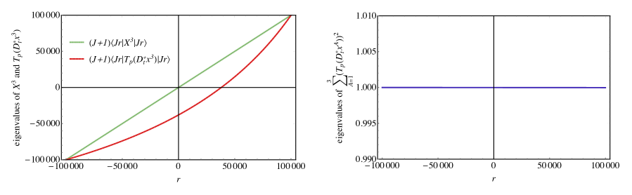
Figure 2: The green dotted line, the red dashed line and the blue solid line show the eigenvalues of $(J+1)X^{3}$, $(J+1)T_{p}(D^{\ast}_{t}x^{3})$ and $\sum_{A}(T_{p}(D^{\ast}_{t}x^{A}))^{2}$ for $J=100000$ and $t=0.4$, respectively.

Approximate diffeomorphism invariants

In this section, we propose three kinds of approximate invariants for the matrix diffeomorphisms on the fuzzy $S^{2}$. These are functions $I(X)$ of the Toeplitz operators $X^{A}=T_{p}(x^{A})$ which satisfy

$$I(X+\delta X)=I(X)+O(p^{-1}),$$ (6.1)

for any infinitesimal matrix diffeomorphism $\delta X$ on the fuzzy $S^{2}$. In particular, if $\delta X$ is an infinitesimal unitary transformation, then they satisfy $I(X+\delta X)=I(X)$.

Invariants from matrix Dirac operator

For $p\times p$ matrices $X^{A}$ $(A=1,2,3)$ and the embedding function $x^{A}$ defined in (5.6), let us define a Dirac type operator,

$$\hat{D}=\sum_{A=1}^{3}\sigma^{A}\otimes(X^{A}-\hat{x}^{A}).$$ (6.2)

Here, we put a hat on $x^{A}$ to emphasize that $\hat{x}^{A}$ are kept fixed when we discuss the variation of approximate invariants, (6.1) ($\hat{x}^{A}$ are equal to $x^{A}$ as functions, $\hat{x}^{A}=x^{A}$.). We also introduce the eigenstates of $\hat{D}$ as

$$\hat{D}\ket*{n}=E_{n}\ket*{n},$$ (6.3)

where the eigenvalues shall be labeled such that $|E_{0}|\leq|E_{1}|\leq|E_{2}|\leq\cdots$. Note that $\hat{D}$, $\ket*{n}$ and $E_{n}$ depend on local coordinates on $S^{2}$ through $\hat{x}^{A}$, although the dependences are not written explicitly. Apart from the fixed embedding function, the operator (6.2) depends only on the matrices $X^{A}$. In this sense, $E_{n}$ and $\ket*{n}$ are functions of $X_{A}$. The eigenvalues $E_{n}$ are not invariant for general transformations of matrices $X^{A}\mapsto X^{{}^{\prime}A}$, but are exactly invariant under the unitary similarity transformations.

In the following, we consider the case in which $X^{A}$ are given by the Toeplitz operators of the embedding function (5.6). By solving the eigenvalue problem for this case [25, 26, 27], one can find that $E_{0}$ and $\ket*{0}$ are given by

$$\begin{split}&E_{0}=\frac{J}{J+1}-1=O(p^{-1}),\\ &|0\rangle=U_{2}\left(\begin{array}[]{c}1\\ 0\\ \end{array}\right)\otimes\ket*{z}.\end{split}$$ (6.4)

Here, $U_{2}=e^{z\sigma^{-}}e^{-\sigma^{3}\text{log}(1+|z|^{2})}e^{-\bar{z}\sigma^{+}}$ is a local rotation matrix and $\ket*{z}$ is the Bloch coherent state (5.4).

The eigenvalue $E_{0}$, which has the smallest absolute value, gives our first example of the approximate invariants. Under an infinitesimal variation $X^{A}\mapsto X^{A}+\delta X^{A}$, $E_{0}$ transforms as

$$\delta E_{0}=\sum^{3}_{A=1}\matrixelement*{0}{\sigma^{A}\otimes\delta X^{A}}{0}.$$ (6.5)

We again emphasize that here $\hat{x}^{A}$ are kept fixed and we consider only the variation of the matrices. Now, suppose that $\delta X^{A}$ is given by a matrix diffeomorphism, which can be written as

$$\delta X^{A}=\frac{p}{2\pi}\int_{S^{2}}\omega\ket*{w}\delta x^{A}(w)\bra*{w},$$ (6.6)

where $\delta x^{A}$ is the variation of $x^{A}$ under a diffeomorphism. Then, (6.5) is evaluated as

$$\delta E_{0}=\sum^{3}_{A=1}x^{A}\delta x^{A}+O(p^{-1}).$$ (6.7)

In deriving (6.7), the following property of the Bloch coherent state is useful:

$$\begin{split}|\innerproduct*{z}{w}|^{2}&=\frac{|1+w\bar{z}|^{4J}}{(1+|z|^{2})^{2J}(1+|w|^{2})^{2J}},\\ &=\exp\left[2J\log\left\{1-\frac{|z-w|^{2}}{(1+|z|^{2})(1+|w|^{2})}\right\}\right],\\ &=\frac{\pi}{2J}(1+|z|^{2})^{2}\delta^{(2)}(z-w)+O(p^{-2}).\end{split}$$ (6.8)

Since $\sum_{A}x^{A}x^{A}=1$, the first term of (6.7) is vanishing. Thus, $E_{0}$ is indeed invariant under the matrix diffeomorphism up to the $1/p$ corrections.

In [28], it was proposed that the matrix Dirac operator can be used to find effective shapes of fuzzy branes. Here, the loci of the zero eigenvalue of the matrix Dirac operator are identified with the effective shape embedded in the flat target space. See also [25, 29]. The same method was also independently proposed in the context of the tachyon condensation in string theory [14, 15, 26].

In [30, 31, 32], to extract the classical shape of noncommutative spaces, another operator $\hat{H}=\sum_{A}(X^{A}-\hat{x}^{A})^{2}/2$ was considered. For matrices which become commuting in the limit of large matrix size, $\hat{H}$ is equivalent to $\hat{D}^{2}$. Thus, the ground state energy of $\hat{H}$ also gives an approximate invariant of the matrix diffeomorphisms.

These invariants have the information of the induced metric for the embedding $\hat{x}^{A}$. As shown in [30], by considering variations of $\hat{x}^{A}$, we can construct from $E_{0}$ the Levi-Civita connection and the Riemann curvature tensor for the induced metric.

Invariants of information metric

In the space of density matrices, one can define the information metric,

$$ds^{2}=\Tr(d\rho G),\quad d\rho=\rho G+G\rho,$$ (6.9)

where $\rho$ is a density matrix and $G$ is determined from $\rho$ by the second equation. One can also restrict oneself to pure states $\{\rho=\outerproduct*{\psi}{\psi}\mid\innerproduct*{\psi}{\psi}=1\}$. In this case, $G=d\rho$ and the metric (6.9) is equivalent to the Fubini-Study metric in the space of all normalized vectors $\{\ket*{\psi}\mid\outerproduct*{\psi}{\psi}=1\}$, which has the structure of the complex projective space.

By using the eigenstate $\ket*{0}$ defined in the previous subsection, let us introduce a density matrix,

$$\rho=\outerproduct*{0}{0}.$$ (6.10)

This gives an embedding of $S^{2}$ into the space of density matrices [27]. Then, the pullback $h$ of the information metric,

$$h_{\mu\nu}d\sigma^{\mu}d\sigma^{\nu}=\Tr d\rho d\rho,$$ (6.11)

gives a metric structure on $S^{2}$.

In our setup, the definition of $h$ depends on the choice of $X^{A}$ and $\hat{x}^{A}$. However, in the setup of [28], $\hat{x}^{A}$ are just thought of as three real parameters and the structure of embedding appears after solving the eigenvalue problem. The underlying space can be defined as the loci of zeros of the matrix Dirac operator. In this sense, the definition of $h$ depends only on the matrices $X^{A}$ and it gives a good geometric object defined in terms of the matrix variables.

Note that $h$ is exactly invariant under unitary similarity transformations $X^{A}\mapsto U^{\dagger}X^{A}U$. Below, we show that the information metric is also approximately covariant under general matrix diffeomorphisms. First, because $E_{0}\rightarrow 0$ $(p\rightarrow\infty)$, we have $\expectationvalue*{\hat{D}^{2}}{0}\rightarrow 0$. This implies that $(X^{A}-\hat{x}^{A})\ket*{0}\rightarrow 0$ for $A=1,2,3$. Let $\delta x^{A}$ be a polynomial of $x^{A}$ with the degree much less than $p$. Then, we also have

$$(\delta X^{A}-\delta x^{A})\ket*{0}\rightarrow 0$$ (6.12)

as $p\rightarrow\infty$, where $\delta X^{A}$ is the Toeplitz operator of $\delta x^{A}$. Let $\delta x^{A}$ be a Lie derivative of $x^{A}$ and $\delta X^{A}$ the corresponding matrix diffeomorphism. Under the matrix diffeomorphism $X^{A}\mapsto X^{A}+\delta X^{A}$, the state $|0\rangle$ transforms as

$$\begin{split}\delta|0\rangle&=\sum_{n\neq 0}\sum^{3}_{A=1}\frac{\outerproduct*{n}{n}\sigma^{A}\otimes\delta X^{A}\ket*{0}}{E_{0}-E_{n}}+\mathrm{i}\delta\lambda\ket*{0},\\ &=\sum_{n\neq 0}\sum^{3}_{A=1}\frac{\outerproduct*{n}{n}\sigma^{A}\ket*{0}\delta x^{A}}{E_{0}-E_{n}}+\mathrm{i}\delta\lambda\ket*{0}+O(p^{-1}),\end{split}$$ (6.13)

where $\delta\lambda$ is a real number and we used (6.12) to obtain the last expression. We again emphasize that we fix $\hat{x}^{A}$ and consider only the variation of $X^{A}$. On the other hand, from the infinitesimal variation of the local coordinates, we obtain

$$\begin{split}\partial_{\mu}|0\rangle=-\sum_{n\neq 0}\sum^{3}_{A=1}\frac{\outerproduct*{n}{n}\sigma^{A}\ket{0}\partial_{\mu}x^{A}}{E_{0}-E_{n}}+\mathrm{i}A_{\mu}\ket*{0},\end{split}$$ (6.14)

where $A=-\mathrm{i}\expectationvalue*{d}{0}$ is the Berry connection. For a diffeomorphism $\delta x^{A}=u^{\mu}\partial_{\mu}x^{A}$, from (6.13) and (6.14), we find

$$\delta\rho=-u^{\mu}\partial_{\mu}\rho+O(p^{-1}).$$ (6.15)

This means that the embedding function $\rho$ transforms as a scalar field under matrix diffeomorphisms. Thus, the induced metric $h$ is also covariant:

$$\delta h_{\mu\nu}=-\nabla_{\mu}u_{\nu}-\nabla_{\nu}u_{\mu}+O(p^{-1}).$$ (6.16)

Diffeomorphism invariants (in the usual sense) defined in terms of $h$ are also approximately invariant under matrix diffeomorphisms. For example, the volume integral $\int_{S^{2}}\sqrt{h}$ or the Einstein-Hilbert action $\int_{S^{2}}\sqrt{h}R$ gives an approximate invariant.

In general, the information metric is different from the induced metric discussed in the previous subsection. For K$\ddot{\text{a}}$hler manifolds, the information metric gives a K$\ddot{\text{a}}$hler metric compatible with the field strength of the Berry connection [31]. Hence, it has intrinsic information on the manifold, which does not depend on the embedding.

Heat kernel on fuzzy sphere

For a $2n$-dimensional closed Riemannian manifold $(M,g)$, the heat kernel,

$$K(t)=\Tr e^{-t\Delta},$$ (6.17)

for the Laplacian, $\Delta=-(1/\sqrt{g})\partial_{\mu}(\sqrt{g}g^{\mu\nu}\partial_{\nu})$, generates diffeomorphism invariants on $M$ as coefficients of the asymptotic expansion in $t\rightarrow+0$:

$$K(t)=\frac{1}{(4\pi t)^{n}}\int_{M}\sqrt{g}+\frac{1}{(4\pi)^{n}t^{n-1}}\int_{M}\sqrt{g}\frac{R}{6}+\cdots.$$ (6.18)

Similarly, we define the heat kernel on the fuzzy $S^{2}$ as

$$\hat{K}(t_{p},p)=\Tr e^{-t_{p}\hat{\Delta}}.$$ (6.19)

Here, $\hat{\Delta}$ is the matrix version of the Laplacian defined by

$$\hat{\Delta}=(J+1)^{2}\sum_{A=1}^{3}[X^{A},[X^{A},\,\cdot\,]]=\sum_{A=1}^{3}[L^{A},[L^{A},\,\cdot\,]],$$ (6.20)

where $X^{A}=T_{p}(x^{A})$ is given in (5.7). See [39, 40] for the properties of $\hat{K}$ for finite size matrices.

It is well-known that the spectrum of $\hat{\Delta}$ coincides with that of the standard Laplacian on $S^{2}$ up to a UV cutoff given by the matrix size. The eigenstates of $\hat{\Delta}$ are given by the fuzzy spherical harmonics $\hat{Y}_{lm}$ [24, 33, 34, 35, 36, 37]. See appendix F for the definition of $\hat{Y}_{lm}$, that we use in the following. For $\hat{Y}_{lm}$, $l$ runs from $0$ to $p-1$ and $m$ runs from $-l$ to $l$. The eigenvalue of $\hat{\Delta}$ is $l(l+1)$ for $\hat{Y}_{lm}$, which coincides with the spectrum of the spherical harmonics on $S^{2}$, except that the angular momentum $l$ has a cutoff $p-1$ for the fuzzy spherical harmonics.

For finite $p$, the spectrum of $\hat{\Delta}$ is finite. Thus, the matrix heat kernel (6.19) has only a regular expansion in $t_{p}\rightarrow+0$ as $\hat{K}=\Tr\textbf{1}_{p^{2}}+O(t_{p})$, which looks trivial and seems not to have any interesting information of the geometry. However, it is obvious that if we first take the large-$p$ limit and then take $t_{p}\rightarrow+0$, $\hat{K}$ should behave similarly to $K$ having a singular expansion. In other words, by putting $t_{p}=p^{-\alpha}$, where $\alpha$ is a small positive number, the heat kernel should have the expansion,

$$\hat{K}(t_{p}=p^{-\alpha},p)=\frac{1}{t_{p}}c_{0}+c_{1}+O(t_{p})$$ (6.21)

in the large-$p$ limit. It follows from the Euler-Maclaurin formula that the coefficients are given by $c_{0}=1$ and $c_{1}=1/3$ for the Laplacian (6.20). See Fig. 3 for the plot of (6.21). The values of $c_{0}$ and $c_{1}$ just coincide with the coefficients of the heat kernel expansion on the continuum $S^{2}$. Thus, in the double scaling limit, the matrix heat kernel possesses geometric information of $S^{2}$.

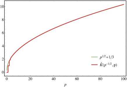
Figure 3: The green dotted line and the red solid line show $p^{1/2}+1/3$ and $\hat{K}$ with $t_{p}=p^{-1/2}$, respectively.

Now, we show that the matrix heat kernel (6.19) is approximately invariant under matrix diffeomorphisms. Let us consider a perturbation $X^{A}\mapsto X^{A}+\delta X^{A}$. Let $\delta X^{A}$ be a general infinitesimal matrix for the moment. (In the end of the calculation, we will restrict $\delta X^{A}$ to be a matrix diffeomorphism.) The eigenvalues of $\hat{\Delta}$ are perturbed by $\delta X^{A}$. Let $\delta_{lm}$ be the deviation of the eigenvalue for the mode $\hat{Y}_{lm}$. From the first order formula of the perturbation theory, one obtains that

$$\delta_{lm}=\frac{(J+1)}{p}\Tr\sum^{3}_{A=1}\left(\hat{Y}^{\dagger}_{lm}[\delta X^{A},[L^{A},\hat{Y}_{lm}]]+\hat{Y}^{\dagger}_{lm}[L^{A},[\delta X^{A},\hat{Y}_{lm}]]\right).$$ (6.22)

The heat kernel (6.19) changes by

$$\delta\hat{K}=-t_{p}\sum_{l=0}^{p-1}\sum_{m=-l}^{l}e^{-t_{p}l(l+1)}\delta_{lm}.$$ (6.23)

The matrix $\delta X^{A}$ can be expanded in terms of the vector fuzzy spherical harmonics as

$$\delta X^{A}=\sum^{p-1}_{l=0}\sum^{l}_{m=-l}\sum^{1}_{\rho=-1}\delta X_{lm\rho}\hat{Y}_{lm\rho}^{A}.$$ (6.24)

Again, see appendix F for the definition of $\hat{Y}_{lm\rho}^{A}$. After an easy calculation, we find that (6.23) is given as

$$\delta\hat{K}=2\mathrm{i}t_{p}\delta X_{00-1}\sqrt{\frac{J+1}{J}}\sum_{l=0}^{p-1}e^{-t_{p}l(l+1)}l(l+1)(2l+1).$$ (6.25)

The important point is that the $\delta\hat{K}$ depends only on $\delta X_{00-1}$. This is exactly the mode proportional to $L^{A}$. This mode changes the radius of $S^{2}$ in the target space, and $\sum_{A}(X^{A}+\delta X^{A})^{2}$ will deviate from the identity matrix even in the large-$p$ limit. Here, recall that, as mentioned in the previous section, any matrix diffeomorphism should keep the relation (5.21). The fluctuation of $\delta X_{00-1}$ violates this constraint, so it is not a matrix diffeomorphism. Therefore, for matrix diffeomorphisms, the matrix heat kernel is invariant. The coefficients in the expansion (6.21) give approximate invariants on fuzzy $S^{2}$.

The matrix Laplacian corresponds to the operator $-\sum_{A}\{x^{A},\{x^{A},\,\cdot\,\}\}$, because of (LABEL:MR). This operator can be written as $-g^{\nu\sigma}\partial_{\nu}\partial_{\sigma}+\cdots$, where $g^{\nu\sigma}=W^{\mu\nu}W^{\rho\sigma}\sum_{A}(\partial_{\mu}x^{A}\partial_{\rho}x^{A})$ and $W^{\mu\nu}$ is the Poisson tensor. The (inverse) metric $g^{\nu\sigma}$ is the open string metric [38] in the strong magnetic flux. Thus, the invariants from the heat kernel are associated with the open string metric.

Summary and Discussion

In this paper, we defined the action of diffeomorphisms on the space of matrices through the matrix regularization. We first constructed the matrix regularization of closed symplectic manifolds based on the Berezin-Toeplitz quantization. We then defined the matrix diffeomorphisms as the matrix regularization of usual diffeomorphisms, as shown in Fig. 1. We finally studied the matrix diffeomorphisms on the fuzzy $S^{2}$ and explicitly constructed holomorphic matrix diffeomorphisms. We also constructed three kinds of approximate invariants of the matrix diffeomorphisms on the fuzzy $S^{2}$. They are associated with three different kinds of metrics, the induced metric, the K$\ddot{\text{a}}$hler metric and the open string metric. In the case of $S^{2}$, they are equivalent up to an overall factor. However, this is not the case for general spaces as shown in [31, 27]. For example, it is easy to see this inequivalence by adding a perturbation to the fuzzy sphere.

The Berezin-Toeplitz quantization gives a systematic construction of the matrix regularization for any compact symplectic manifold. In the construction of Toeplitz operators that we discussed in this paper, $\text{spin}^{c}$ structures play an essential role. We emphasize that the existence of the symplectic structure is not essential in this construction. In fact, Toeplitz operators can also be constructed for $S^{4}$ [27, 41, 42], which is not a symplectic manifold. Here, the well-known configuration of the fuzzy $S^{4}$ [43] is obtained as the Toeplitz operator of the standard embedding function $S^{4}\rightarrow\textbf{R}^{5}$. It is known that any four dimensional oriented smooth manifold is a $\text{spin}^{c}$ manifold. Hence, Toeplitz operators can be constructed for any four-dimensional compact Riemannian manifolds.

In the matrix model formulation of M-theory, the fuzzy $S^{4}$ is interpreted as a longitudinal fivebrane [43]. This example shows that the matrix model contains not only symplectic manifolds but also more general manifolds with $\text{spin}^{c}$ structures. (Note that any D-brane must have a $\text{spin}^{c}$ structure.) For general $\text{spin}^{c}$ manifolds without Poisson structure, the second condition in (LABEL:MR) for the matrix regularization can not be defined. However, the construction of Toeplitz operators is always possible and this may give a more fundamental framework of characterizing the matrix model.

Although we focused only on $S^{2}$ in this paper, our formulation can be straightforwardly extended to other spaces. It will be important to study more general examples, in order to understand the properties of matrix diffeomorphisms. For example, the correspondence between area-preserving diffeomorphisms and unitary similarity transformations may be more nontrivial for general cases. When the first cohomology class is trivial, any area-preserving diffeomorphism can be written in the form (2.4) and this is realized as a unitary similarity transformation in our definition of the matrix diffeomorphisms. However, when the first cohomology class is nontrivial, there exist other area-preserving diffeomorphisms which cannot be written in the form (2.4). It is interesting to study matrix diffeomorphisms corresponding to such general area-preserving diffeomorphisms.

The approximate invariants we proposed in this paper are purely defined in terms of the matrix configuration of the fuzzy $S^{2}$. We consider that the constructions in section 6.1 and 6.2 can be generalized to the case of an arbitrary $\text{spin}^{c}$ manifold. Such generalization may enable us to construct gravitational theories on fuzzy spaces. It is intriguing to pursue this direction.

Appendix A Berezin-Toeplitz quantization for classical mechanics

In this appendix, we consider the Berezin-Toeplitz quantization of a classical mechanical system of a particle on the real line.

We introduce a complex coordinate $z=(q+\mathrm{i}p)/\sqrt{2}$ for the canonical variables $(q,p)\in\textbf{R}^{2}$. We define a symplectic form on $\textbf{R}^{2}$ by $\omega=dq\wedge dp=\mathrm{i}dz\wedge d\bar{z}$. Then, the Poisson bracket defined by $\omega$ satisfies $\{q,p\}=\mathrm{i}\{z,\bar{z}\}=1$.

Classical observables are just smooth functions on the phase space, $\{f(z,\bar{z})\in C^{\infty}(\mathbf{R}^{2})\}$. The problem of the quantization is then to find a map from the classical observables to quantum observables $\{\hat{f}\}$, which is a set of operators on a Hilbert space. It must be required that $\{f,g\}$ is mapped to $[\hat{f},\hat{g}]/\mathrm{i}\hbar$ up to higher order corrections of $\hbar$, where $\hat{f}$ and $\hat{g}$ are the images of $f$ and $g$, respectively. One can find such a map starting from the canonical operators $(\hat{q},\hat{p})$ satisfying $[\hat{q},\hat{p}]=\mathrm{i}\hbar$ and then fix the ordering of $(\hat{q},\hat{p})$ in composite operators.

Each ordering gives a different quantization scheme. Among those, let us consider the anti-normal ordering. From $(\hat{q},\hat{p})$, one can define the creation and annihilation operators $\hat{a},\hat{a}^{\dagger}$ satisfying $[\hat{a},\hat{a}^{\dagger}]=1$. In the anti-normal ordering, $\hat{a}$ and $\hat{a}^{\dagger}$ are put on the left and right sides, respectively. Let $\ket{0}$ be the vacuum state defined by $\hat{a}\ket{0}=0$. Then, the quantization map associated with this ordering can be written as

$$\hat{f}=T_{1/\hbar}(f)=\frac{1}{\pi\hbar}\int_{\mathbf{R}^{2}}\omega\ket*{z}f(z,\bar{z})\bra*{z}$$ (A.1)

for $f\in C^{\infty}(\textbf{R}^{2})$, where $\ket*{z}=e^{-|z|^{2}/2\hbar}e^{z\hat{a}^{\dagger}/\sqrt{\hbar}}\ket*{0}$ is the canonical coherent state. The overall factor $1/\pi\hbar$ is chosen such that $T_{1/\hbar}(1)=1$ holds. It is easy to check that this map satisfies the similar conditions to (LABEL:MR).

There is a very useful reformulation of (A.1) in terms of Dirac zero modes. Let us consider the $U(1)$ gauge potential $A=(qdp-pdq)/2$ for the constant magnetic flux. The covariant Dirac operator is given by

$$D=\mathrm{i}\sigma^{a}\biggl{(}\partial_{a}-\frac{\mathrm{i}}{\hbar}A_{a}\biggr{)},$$ (A.2)

where $\sigma^{a}$ $(a=1,2)$ is the Pauli matrix. The orthonormal basis of the Dirac zero modes is given by

$$\psi_{i}(z,\bar{z})=\frac{1}{\sqrt{\pi\hbar}}\left(\begin{array}[]{c}\innerproduct*{i}{z}\\ 0\end{array}\right),$$ (A.3)

where $\{\ket{i}\mid i=1,2,\cdots\}$ is any orthonormal basis of the Hilbert space. In terms of the zero modes (A.3), we can rewrite (A.1) as

$$\matrixelement{i}{T_{1/\hbar}(f)}{j}=\int_{\textbf{R}^{2}}\omega\,\psi^{\dagger}_{j}(z,\bar{z})f(z,\bar{z})\psi_{i}(z,\bar{z})\,.$$ (A.4)

Note that the coherent states in (A.1) are represented as the covariant spinors in (A.4).

The operator ${T_{1/\hbar}(f)}$ is called the Toeplitz operator of $f$. In the form of (A.4), the Toeplitz operator is given by the restriction of $f$ onto the space of the Dirac zero modes. The zero modes (A.3) are the wave functions in the lowest Landau level of the Hamiltonian for a charged particle moving in a constant magnetic field. Thus, one can also say that the Toeplitz operator is the restriction of functions onto the space of the lowest Landau level.

The basic data required for constructing (A.4) are the Riemannian metric, the $U(1)$ gauge field and the Dirac zero modes. A big advantage for using spinors is that the same construction works also for more general manifolds.

Appendix B Estimation of $\text{dim}\text{Ker}D$

In this appendix, we show that the sequence $N_{p},N_{p+1},\ldots$ defined in section 3 is strictly monotonically increasing for large $p$.

Let us define the chirality operator $\gamma_{2n+1}=(-\mathrm{i})^{n}\gamma_{1}\gamma_{2}\cdots\gamma_{2n}$. Since $\gamma_{2n+1}$ is Hermitian and satisfies $\gamma_{2n+1}^{2}=\textbf{1}_{2^{n}}$, we can decompose $W$ into the direct sum of the eigenspaces $W^{\pm}$ with the eigenvalues $\pm 1$. Correspondingly, we have the decomposition $S\otimes L_{p}=(S^{+}\otimes L_{p})\oplus(S^{-}\otimes L_{p})$ where $S^{\pm}$ are the sub bundles of $S$ with fibers $W^{\pm}$. Since $D\gamma_{2n+1}=-\gamma_{2n+1}D$, we have $D\psi\in\Gamma(S^{\mp}\otimes L_{p})$ for $\psi\in\Gamma(S^{\pm}\otimes L_{p})$. Hence, $D$ has the form

$$D=\left(\begin{array}[]{cc}0&D^{-}\\ D^{+}&0\end{array}\right),$$ (B.1)

where $D^{\pm}$ are the restrictions of $D$ to $\Gamma(S^{\pm}\otimes L_{p})$. We define the subspaces of $\text{Ker}D$ by $\text{Ker}D^{\pm}=\text{Ker}D\cap\Gamma(S^{\pm}\otimes L_{p})$. Since (B.1) implies that $\text{dim}\text{Ker}D=\text{dim}\text{Ker}D^{+}+\text{dim}\text{Ker}D^{-}$, we have

$$\text{dim}\text{Ker}D\geq|\text{ind}D|,$$ (B.2)

where $\text{ind}D=\text{dim}\text{Ker}D^{+}-\text{dim}\text{Ker}D^{-}$ is the index of $D$. The equal sign holds if and only if $\text{dim}\text{Ker}D^{+}=0$ or $\text{dim}\text{Ker}D^{-}=0$. In addition, $\text{Ker}D^{-}=\{0\}$ holds in our setting for large $p$ because of the vanishing theorem [23], so that we have

$$\text{dim}\text{Ker}D=|\text{ind}D|.$$ (B.3)

Moreover, the Atiyah-Singer index theorem gives a relation,

$$\text{ind}D=\int_{M}\hat{A}(M)\wedge\text{ch}(L_{p}),$$ (B.4)

where $\hat{A}(M)$ denotes the $\hat{A}$-genus of $M$ and $\text{ch}(L_{p})$ the Chern character of $L_{p}$. Then, we have the formula,

$$\text{ch}(L_{p})=(\text{ch}(L_{1}))^{p}=\text{exp}\biggl{(}\frac{pF}{2\pi}\biggr{)},$$ (B.5)

where the product of differential forms is defined by the wedge product. From the assumption that $F/2\pi=\omega V_{n}^{-1/n}$, we find

$$\text{ind}D=p^{n}+O(p^{n-2}).$$ (B.6)

From (B.3) and (B.6), we conclude that $\{N_{p}=\text{dim}\text{Ker}D\mid p\gg 1\}$ is indeed a strictly monotonically increasing sequence.

Appendix C Geometric structures on $S^{2}$

In this appendix, we review our notation for the geometry of $S^{2}$ and introduce some geometric structures.

Let $x^{A}$ $(A=1,2,3)$ be the Cartesian coordinates on $\mathbf{R}^{3}$. We consider a two-dimensional unit sphere $S^{2}$ defined by the equation $\sum_{A=1}^{3}x^{A}x^{A}=1$. We identify $S^{2}$ with the Riemann sphere $\hat{\mathbf{C}}=\mathbf{C}\cup\{\infty\}$ by the stereographic projection $S^{2}\to\hat{\mathbf{C}}$ defined by

$$z=\frac{x^{1}+\mathrm{i}x^{2}}{1+x^{3}}$$ (C.1)

for $x^{3}\neq-1$ and $z=\infty$ for $x^{3}=-1$. Under this identification, we can cover $S^{2}$ by two open subsets $U_{z}:=\hat{\mathbf{C}}-\{\infty\}$ and $U_{w}:=\hat{\mathbf{C}}-\{0\}$. Then, the coordinate neighborhood system of $S^{2}$ consists of $(U_{z};z)$ and $(U_{w};w:=1/z)$. The coordinate transformation from $(U_{z};z)$ to $(U_{w};w)$ is given by a holomorphic map $z\mapsto 1/z$.

The sphere $S^{2}$ is a K$\ddot{\text{a}}$hler manifold and we can define a symplectic structure $\omega$, complex structure $J$ and Riemann structure $g$ such that they satisfy the compatible condition. First, we define $\omega$ by a volume form on $S^{2}$,

$$\omega=\mathrm{i}\frac{dz\wedge d\bar{z}}{(1+|z|^{2})^{2}},$$ (C.2)

such that $\int_{S^{2}}\omega=2\pi$. Secondly, we define $J$ by $J(\partial_{z})=\mathrm{i}\partial_{z}$ and $J(\partial_{\bar{z}})=-\mathrm{i}\partial_{\bar{z}}$. The local form is

$$J=\mathrm{i}\partial_{z}\otimes dz-\mathrm{i}\partial_{\bar{z}}\otimes d\bar{z}.$$ (C.3)

Finally, we define $g$ by the compatible condition $g(\,\cdot\,,\,\cdot\,)=\omega(\,\cdot\,,J\,\cdot\,)$ as

$$g=2\frac{dzd\bar{z}}{(1+|z|^{2})^{2}}.$$ (C.4)

We choose an orthonormal frame on $U_{z}$ with respect to the metric (C.4) as

$$\begin{split}e_{1}&=\frac{1}{\sqrt{2}}(1+|z|^{2})(\partial_{z}+\partial_{\bar{z}}),\\ e_{2}&=\frac{\mathrm{i}}{\sqrt{2}}(1+|z|^{2})(\partial_{z}-\partial_{\bar{z}}).\end{split}$$ (C.5)

Then, the dual basis is

$$\begin{split}\theta^{1}&=\frac{1}{\sqrt{2}}\frac{dz+d\bar{z}}{1+|z|^{2}},\\ \theta^{2}&=\frac{1}{\sqrt{2}\mathrm{i}}\frac{dz-d\bar{z}}{1+|z|^{2}}.\end{split}$$ (C.6)

The linear map (3.3) is given by

$$\gamma(e_{a})=\sigma_{a},$$ (C.7)

where $\sigma_{a}$ are Pauli matrices. In this choice, the chirality operator is $\Gamma=-\mathrm{i}\sigma_{1}\sigma_{2}=\sigma_{3}$. The condition (LABEL:spin_connection), which determines the spin connection on $S$, is equivalent to

$$\begin{split}&\Omega^{1}{}_{2}\wedge\theta^{2}-\frac{\mathrm{i}}{\sqrt{2}}(z-\bar{z})\theta^{1}\wedge\theta^{2}=0,\\ &\Omega^{1}{}_{2}\wedge\theta^{1}-\frac{1}{\sqrt{2}}(z+\bar{z})\theta^{2}\wedge\theta^{1}=0.\end{split}$$ (C.8)

By solving these equation, we obtain

$$\Omega^{1}{}_{2}=\frac{\mathrm{i}}{\sqrt{2}}(z-\bar{z})\theta^{1}+\frac{1}{\sqrt{2}}(z+\bar{z})\theta^{2}=-\mathrm{i}\frac{\bar{z}dz-zd\bar{z}}{1+|z|^{2}}.$$ (C.9)

We also need a topologically nontrivial configuration of the $U(1)$ gauge connection on $S^{2}$ to construct Toeplitz operators. We use the Wu-Yang monopole configuration,

$$A^{(z)}=-\frac{\mathrm{i}}{2}\frac{\bar{z}dz-zd\bar{z}}{1+|z|^{2}},$$ (C.10)

for $U_{z}$. On the overlap of two patches, the gauge connection $A^{(w)}$ on $U_{w}$ is related to (C.10) by a $U(1)$ gauge transformation. More specifically, $A^{(w)}=A^{(z)}-d\,\text{arg}(z)$ on $U_{z}\cap U_{w}$. This gauge connection satisfies $F=dA^{(z)}=2\pi\omega V_{1}^{-1}$.

Appendix D Automorphisms on $S^{2}$

In this appendix, we review $\text{Aut}(S^{2},J)$, $\text{Aut}(S^{2},g)$ and $\text{Aut}(S^{2},\omega)$. See appendix C for the definitions of $J$, $g$ and $\omega$.

$\text{Aut}(S^{2},J)$

First, we consider $\text{Aut}(S^{2},J)$. For $\varphi\in\text{Diff}(S^{2})$, let $\hat{z}$ be a point on $S^{2}$ such that $\varphi(\hat{z})=\infty$. Namely, $\hat{z}$ is a pole of $\varphi$. Note that since $\varphi$ needs to be one-to-one, $\hat{z}$ is the unique pole. For simplicity, we first suppose that $\hat{z}=\infty$. In this case, we have $\varphi(U_{z})\subset U_{z}$. The local form of the new tensor field $J^{\prime}$ induced by $\varphi$ is given on $U_{z}$ as

$$J^{\prime}=\mathrm{i}\varphi^{-1}_{\ast}(\partial_{z})\otimes\varphi^{\ast}(dz)-\mathrm{i}\varphi^{-1}_{\ast}(\partial_{\bar{z}})\otimes\varphi^{\ast}(d\bar{z}),$$ (D.1)

where $\varphi_{\ast}$ is the pushforward by $\varphi$. If $J^{\prime}=J$, then we have

$$\begin{split}&\partial_{\varphi}z\,\partial_{z}\varphi-\partial_{\bar{\varphi}}z\,\partial_{z}\bar{\varphi}=1,\\ &\partial_{\varphi}\bar{z}\,\partial_{z}\varphi-\partial_{\bar{\varphi}}\bar{z}\,\partial_{z}\bar{\varphi}=0,\end{split}$$ (D.2)

where $\partial_{\varphi}=\partial/\partial\varphi(z)$. Note that $\varphi(z)$ generally depends on both $z$ and $\bar{z}$. From the chain rule, $1=\partial_{z}z=\partial_{\varphi}z\,\partial_{z}\varphi+\partial_{\bar{\varphi}}z\,\partial_{z}\bar{\varphi}$, and the first equation of (LABEL:condition_for_preserve_J), the relation $\partial_{\bar{\varphi}}z\,\partial_{z}\bar{\varphi}=0$ follows. This shows that $\varphi(z)$ and $\varphi^{-1}(z)$ are holomorphic on $U_{z}$. The second equation of (LABEL:condition_for_preserve_J) automatically holds when $\partial_{z}\bar{\varphi}=\partial_{\bar{\varphi}}z=0$. In the case that $\hat{z}\neq\infty$, a similar argument leads to the conclusion that $\varphi$ has a pole at $\hat{z}$ and is holomorphic at every points except at $\hat{z}$. In summary, $\varphi$ preserving $J$ is a meromorphic function on $S^{2}$ with a pole at a point.

One can express such $\varphi$ as $\varphi=f/h$, where $f$ and $h$ are relatively prime functions on $S^{2}$. If the degree of $f$ or $h$ is second or higher, $\varphi$ cannot be one-to-one. Thus, both of $f$ and $h$ have to be at most linear polynomials and $\varphi\in\text{Aut}(S^{2},J)$ is expressed as

$$\varphi(z)=\frac{az+b}{cz+d},$$ (D.3)

where $a,b,c,d$ are complex numbers such that $ad-bc\neq 0$. We define $\varphi(\infty)=\infty$ for $c=0$ and $\varphi(\infty)=a/c$ for $c\neq 0$. Since multiplying $a,b,c,d$ by a common number does not change the value of (D.3), we can fix $ad-bc=1$. This transformation is the so-called M$\ddot{\text{o}}$bius transformation and the group $\text{Aut}(S^{2},J)$ consists of all M$\ddot{\text{o}}$bius transformations.

Let us consider a homomorphism $\Pi:SL(2,\mathbf{C})\to\text{Aut}(S^{2},J)$ defined by

$$\left(\begin{array}[]{cc}a&b\\ c&d\end{array}\right)\mapsto\varphi.$$ (D.4)

Then, we have $\text{Ker}\Pi=\{\pm\textbf{1}_{2}\}$. From the fundamental theorem on homomorphisms, we find that $\text{Aut}(S^{2},J)$ is isomorphic to $PSL(2,\mathbf{C})=SL(2,\mathbf{C})/\mathbf{Z}_{2}$.

$\text{Aut}(S^{2},g)$

Secondly, we consider $\text{Aut}(S^{2},g)$. We suppose that $\hat{z}=\infty$ again. The local form of the new tensor field $g^{\prime}$ induced by $\varphi$ on $U_{z}$ is given by

$$g^{\prime}=2\frac{\varphi^{\ast}(dz)\varphi^{\ast}(d\bar{z})}{(1+|\varphi(z)|^{2})^{2}}.$$ (D.5)

If $g^{\prime}=g$, then we have

$$\begin{split}&\partial_{\bar{z}}\varphi\,\partial_{\bar{z}}\bar{\varphi}=0,\\ &\partial_{z}\varphi\,\partial_{\bar{z}}\bar{\varphi}+\partial_{\bar{z}}\varphi\,\partial_{z}\bar{\varphi}=\frac{(1+|\varphi(z)|^{2})^{2}}{(1+|z|^{2})^{2}}.\end{split}$$ (D.6)

From the first equation of (LABEL:condition_for_preserve_metric), $\partial_{\bar{z}}\varphi=0$ or $\partial_{\bar{z}}\bar{\varphi}=0$ follows. The former and the later means that $\varphi$ is holomorphic and anti-holomorphic on $U_{z}$, respectively.

In the case that $\varphi$ is holomorphic, the same argument as $\text{Aut}(S^{2},J)$ shows that $\varphi$ is given by the M$\ddot{\text{o}}$bius transformation (D.3). In the case that $\varphi$ is anti-holomorphic, we can set $\varphi=\tilde{\varphi}\circ\theta$, where $\theta\in\text{Diff}(S^{2})$ is defined by $\theta(z)=\bar{z}$ and $\tilde{\varphi}\in\text{Diff}(S^{2})$ is holomorphic on $U_{z}$. Then, $\tilde{\varphi}$ is given by the M$\ddot{\text{o}}$bius transformation (D.3), so that $\varphi$ can be written as

$$\varphi(z)=\frac{a\bar{z}+b}{c\bar{z}+d},$$ (D.7)

where the definition of $\{a,b,c,d\}$ is the same as (D.3). This transformation is called an anti-M$\ddot{\text{o}}$bius transformation. The composition of two anti-M$\ddot{\text{o}}$bius transformations is a M$\ddot{\text{o}}$bius transformation, and the composition of a M$\ddot{\text{o}}$bius transformation and an anti-M$\ddot{\text{o}}$bius transformation is an anti-M$\ddot{\text{o}}$bius transformation. Thus, all M$\ddot{\text{o}}$bius transformations and anti-M$\ddot{\text{o}}$bius transformations form a group, which is called the extended M$\ddot{\text{o}}$bius group and denoted by $\overline{PSL}(2,\mathbf{C})$.

In any case, the second equation of (LABEL:condition_for_preserve_metric) is equivalent to

$$\begin{split}|a|^{2}+|c|^{2}=|b|^{2}+|d|^{2}=1,\quad a\bar{b}+c\bar{d}=0.\end{split}$$ (D.8)

This means that both $\Pi^{-1}(\varphi)$ and $\Pi^{-1}(\tilde{\varphi})$ are elements of $PSU(2,\mathbf{C})=SU(2,\mathbf{C})/{\bf\it Z}_{2}$. We therefore find that $\text{Aut}(S^{2},g)$ is isomorphic to $\overline{PSU}(2,\mathbf{C})$ which is a subgroup of $\overline{PSL}(2,\mathbf{C})$ defined by the condition (D.8). We also find that $\text{Aut}(S^{2},J,g)$ is isomorphic to $PSU(2,\mathbf{C})\cong SO(3)$.

Note that $\text{Aut}(S^{2},J,g)=\text{Aut}(S^{2},\omega,J,g)$, since $J$ and $g$ are compatible with $\omega$.

$\text{Aut}(S^{2},\omega)$

Finally, we consider $\text{Aut}(S^{2},\omega)$. The local form of the new tensor field $\omega^{\prime}$ induced by $\varphi$ on $U_{z}$ is given by

$$\omega^{\prime}=\mathrm{i}\frac{\varphi^{\ast}(dz)\wedge\varphi^{\ast}(d\bar{z})}{(1+|\varphi(z)|^{2})^{2}}.$$ (D.9)

If $\omega^{\prime}=\omega$, then we have

$$\partial_{z}\varphi\,\partial_{\bar{z}}\bar{\varphi}-\partial_{\bar{z}}\varphi\,\partial_{z}\bar{\varphi}=\frac{(1+|\varphi(z)|^{2})^{2}}{(1+|z|^{2})^{2}}.$$ (D.10)

Note that there is not an equation corresponding to the first equation of (LABEL:condition_for_preserve_metric). We therefore cannot conclude that $\varphi$ is holomorphic or anti-holomorphic on $U_{z}$. This suggests that $\text{Aut}(S^{2},\omega)$ is a larger group than $\text{Aut}(S^{2},J)$ and $\text{Aut}(S^{2},g)$. In fact, as reviewed in section 2, the Lie algebra of $\text{Aut}(S^{2},\omega)$ is isomorphic to the Poisson algebra on $S^{2}$, since the first cohomology class on $S^{2}$ is trivial. If $\varphi$ is holomorphic, satisfying (D.10) is equivalent to $\varphi\in\text{Aut}(S^{2},\omega,g,J)$. If $\varphi$ is anti-holomorphic, (D.10) never holds. This corresponds to the fact that the orientation determined by $\omega$ is not kept under the inversions $z\mapsto\bar{z}$.

Appendix E Matrix diffeomorphisms for $\text{Aut}(S^{2},\omega,J,g)$

In this appendix, we show that matrix diffeomorphisms for $\text{Aut}(S^{2},\omega,J,g)$ can be written as unitary similarity transformations.

For any $\varphi\in\text{Aut}(S^{2},\omega,J,g)$, there exists an element $u\in SU(2,\mathbf{C})$ such that $\varphi=\Pi(u)$, where $\Pi$ is defined by (D.4). By using the relation of the stereographic coordinate (C.1), it is easy to check that the following relation holds:

$$\varphi^{\ast}x^{A}=\sum^{3}_{B=1}\Lambda^{AB}x^{B},$$ (E.1)

where $\Lambda\in SO(3)$ is the three dimensional irreducible representation of $u$. There exists a unitary matrix $U$ (given by the $p$-dimensional representation of $u$) such that $\sum_{B}\Lambda^{AB}L^{B}=UL^{A}U^{-1}$. Hence, we find that

$$\matrixelement{i}{T_{p}(\varphi^{\ast}x^{A})}{j}=\sum^{3}_{B=1}\Lambda^{AB}\matrixelement*{i}{X^{B}}{j}=\matrixelement*{i}{UX^{A}U^{-1}}{j}.$$ (E.2)

In conclusion, any matrix diffeomorphism corresponding to $\varphi\in\text{Aut}(S^{2},J,g)$ is a unitary similarity transformation.

Appendix F Fuzzy spherical harmonics

In this appendix, we review the definition of the fuzzy spherical harmonics and the vector fuzzy spherical harmonics. See [36, 37] for more details.

The linear maps $[L^{A},\,\cdot\,]$ on $M_{p}(\mathbf{C})$ define a $p^{2}$-dimensional representation of the generators of $SU(2)$ because they satisfy $[[L^{A},\,\cdot\,],[L^{B},\,\cdot\,]]=\mathrm{i}\sum^{3}_{C=1}\epsilon^{ABC}[L^{C},\,\cdot\,]$. The fuzzy spherical harmonics $\hat{Y}_{lm}$ $(l=0,1,\ldots,p-1,m=-l,-l+1,\ldots,l)$ are defined as the standard basis of this representation space which satisfy

$$\begin{split}&[L^{\pm},\hat{Y}_{lm}]=\sqrt{(l\mp m)(l\pm m+1)}\hat{Y}_{lm\pm 1},\\ &[L^{3},\hat{Y}_{lm}]=m\hat{Y}_{lm},\end{split}$$ (F.1)

and the orthonormality condition $\Tr\hat{Y}^{\dagger}_{lm}\hat{Y}_{l^{\prime}m^{\prime}}/p=\delta_{ll^{\prime}}\delta_{mm^{\prime}}$. They are expressed in terms of the basis $\{\outerproduct*{Jr}{Jr^{\prime}}\mid r,r^{\prime}=-J,-J+1,\ldots,J\}$ as

$$\hat{Y}_{lm}=\sqrt{p}\sum^{J}_{r,r^{\prime}=-J}(-1)^{-J+r^{\prime}}C^{lm}_{JrJ-r^{\prime}}\outerproduct*{Jr}{Jr^{\prime}},$$ (F.2)

where $C^{lm}_{JrJ-r^{\prime}}$ is the Clebsch-Gordan coefficient.

The vector fuzzy spherical harmonics $\hat{Y}^{A}_{lm\rho}$ $(\rho=-1,0,1)$ are defined in terms of the fuzzy spherical harmonics as

$$\hat{Y}^{A}_{lm\rho}=\mathrm{i}^{\rho}\sum_{B=1}^{3}\sum_{n=-\tilde{Q}}^{\tilde{Q}}V^{AB}C^{Qm}_{\tilde{Q}n1B}\hat{Y}_{\tilde{Q}n},$$ (F.3)

where $Q=l+\delta_{\rho 1}$, $\tilde{Q}=l+\delta_{\rho-1}$ and $V$ is a unitary matrix given by

$$V=\left(\begin{array}[]{ccc}-1&0&1\\ -\mathrm{i}&0&-\mathrm{i}\\ 0&\sqrt{2}&0\end{array}\right).$$ (F.4)

They also satisfy the orthonormality condition $\sum^{3}_{A=1}\Tr\hat{Y}^{A\dagger}_{lm\rho}\hat{Y}^{A}_{l^{\prime}m^{\prime}\rho^{\prime}}/p=\delta_{ll^{\prime}}\delta_{mm^{\prime}}\delta_{\rho\rho^{\prime}}$ and transform as the vector representation under $SU(2)$ rotation.

References

- [1] J. Hoppe, "Quantum theory of a relativistic surface and a two-dimensional bound state ploblem," Ph. D. thesis. MIT (1982)
- [2] B. de Wit, J. Hoppe and H. Nicolai, Nucl. Phys. B 305, 545 (1988).
- [3] T. Banks, W. Fischler, S. H. Shenker and L. Susskind, Phys. Rev. D 55, 5112 (1997).
- [4] N. Ishibashi, H. Kawai, Y. Kitazawa and A. Tsuchiya, Nucl. Phys. B 498, 467 (1997).
- [5] M. Hanada, H. Kawai and Y. Kimura, Prog. Theor. Phys. 114, 1295 (2006).
- [6] A. H. Chamseddine and A. Connes, Commun. Math. Phys. 186, 731 (1997).
- [7] P. Aschieri, M. Dimitrijevic, F. Meyer and J. Wess, Class. Quant. Grav. 23, 1883 (2006).
- [8] H. Steinacker, Class. Quant. Grav. 27, 133001 (2010).
- [9] V. P. Nair, Phys. Rev. D 92, no. 10, 104009 (2015).
- [10] S. Klimek and A. Lesniewski, Comm. Math. Phys. 146, no. 1, 103-122 (1992).
- [11] M. Bordemann, E. Meinrenken and M. Schlichenmaier, Commun. Math. Phys. 165, 281 (1994).
- [12] X. Ma and G. Marinescu, J. Geom. Anal. 18, 565-611 (2008).
- [13] T. Asakawa, S. Sugimoto and S. Terashima, JHEP 0203, 034 (2002).
- [14] S. Terashima, JHEP 0510, 043 (2005).
- [15] S. Terashima, JHEP 1807, 008 (2018).
- [16] I. Ellwood, JHEP 0508, 078 (2005).
- [17] K. Hasebe, Int. J. Mod. Phys. A 31, no. 20n21, 1650117 (2016).
- [18] K. Hasebe, Nucl. Phys. B 934, 149 (2018).
- [19] S. Kobayashi, “Transformation Groups in Differential Geometry,” Springer-Verlag, Berlin (1972).
- [20] J. M. Gracia-Bondia, J. C. Vrilly and H. Figueroa, “Elements of Noncommutative Geometry,” Birkhuser, Boston (2001).
- [21] J. Arnlind, J. Hoppe and G. Huisken, J. Diff. Geom. 91, no. 1, 1 (2012).
- [22] N. M. J. Woodhouse, “Geometric Quantization,” Clarendon Press, Oxford (1992).
- [23] X. Ma and G. Marinescu, Math. Z. 240, no. 3, 651-664 (2002).
- [24] J. Madore, Class. Quant. Grav. 9, 69 (1992).
- [25] M. H. de Badyn, J. L. Karczmarek, P. Sabella-Garnier and K. H. C. Yeh, JHEP 1511, 089 (2015).
- [26] T. Asakawa, G. Ishiki, T. Matsumoto, S. Matsuura and H. Muraki, PTEP 2018, no. 6, 063B04 (2018).
- [27] G. Ishiki, T. Matsumoto and H. Muraki, Phys. Rev. D 98, no. 2, 026002 (2018).
- [28] D. Berenstein and E. Dzienkowski, Phys. Rev. D 86, 086001 (2012).
- [29] J. L. Karczmarek and K. H. C. Yeh, JHEP 1511, 146 (2015).
- [30] G. Ishiki, Phys. Rev. D 92, no. 4, 046009 (2015).
- [31] G. Ishiki, T. Matsumoto and H. Muraki, JHEP 1608, 042 (2016).
- [32] L. Schneiderbauer and H. C. Steinacker, J. Phys. A 49, no. 28, 285301 (2016).
- [33] H. Grosse, C. Klimcik and P. Presnajder, Commun. Math. Phys. 178, 507 (1996).
- [34] S. Baez, A. P. Balachandran, B. Ydri and S. Vaidya, Commun. Math. Phys. 208, 787 (2000).
- [35] K. Dasgupta, M. M. Sheikh-Jabbari and M. Van Raamsdonk, JHEP 0205, 056 (2002).
- [36] G. Ishiki, S. Shimasaki, Y. Takayama and A. Tsuchiya, JHEP 0611, 089 (2006).
- [37] T. Ishii, G. Ishiki, S. Shimasaki and A. Tsuchiya, Phys. Rev. D 78, 106001 (2008).
- [38] N. Seiberg and E. Witten, JHEP 9909, 032 (1999).
- [39] N. Sasakura, JHEP 0412, 009 (2004).
- [40] N. Sasakura, JHEP 0503, 015 (2005).
- [41] S. C. Zhang and J. p. Hu, Science 294, 823 (2001).
- [42] K. Hasebe, SIGMA 6, 071 (2010).
- [43] J. Castelino, S. Lee and W. Taylor, Nucl. Phys. B 526, 334 (1998).