The molecular-gas properties in the gravitationally lensed merger HATLAS J142935.3-002836
Abstract
Follow-up observations of (sub-)mm-selected gravitationally-lensed systems have allowed a more detailed study of the dust-enshrouded phase of star-formation up to very early cosmic times. Here, the case of the gravitationally-lensed merger in HATLAS J142935.3-002836 (also known as H; , ) is revisited following recent developments in the literature and new APEX observations targeting two carbon monoxide (CO) rotational transitions Jup=3 and 6. We show that the line-profiles comprise three distinct velocity components, where the fainter high-velocity one is less magnified and more compact. The modelling of the observed spectral line energy distribution of CO Jup=2 to 6 and [CI] assumes a large velocity gradient scenario, where the analysis is based on four statistical approaches. Since the detected gas and dust emission comes exclusively from only one of the two merging components (the one oriented North-South, NS), we are only able to determine upper-limits for the companion. The molecular gas in the NS component in H is found to have a temperature of 70 K, a volume density of , to be expanding at 10 km/s/pc, and amounts to . The CO to H2 conversion factor is estimated to be M⊙/(K km/s pc. The NS galaxy is expected to have a factor of more gas than its companion ( M⊙). Nevertheless, the total amount of molecular gas in the system comprises only up to 15 per cent ( upper-limit) of the total (dynamical) mass.
keywords:
Gravitational lensing: strong – Galaxies: interactions — Submillimeter: galaxies — Submillimeter: ISM – ISM: abundances1 Introduction
Understanding the life cycle of galaxies necessitates an observational multi-wavelength approach, not only due to the many evolution tracks a galaxy may follow (e.g., finishing as an early-type galaxy, or as an “untouched” disc galaxy as NGC 1277, Trujillo et al., 2014), but also the many physical mechanisms at play (e.g., star-formation and its quenching, heavy elements production), and the advantages and disadvantages specific to different methods of analysis.
Specifically, the brightest of the dusty star-forming galaxies (DSFGs; Casey et al., 2014, for a review), also referred to as Sub-Millimetre Galaxies (SMGs; Smail et al., 1997; Hughes et al., 1998), provide a strong case for the early active evolution stages of the most massive galaxies seen in the local Universe (e.g., Simpson et al., 2014; Toft et al., 2014). Despite not being representative of the whole galaxy population, SMGs may enable us to unveil the dusty origins of the local Universe’s massive monsters, as seen in a Universe with less than 25 per cent its current age (). They are highly star-forming and already massive galaxies, quickly exhausting their large gas reservoirs, and with a source density comparable to massive galaxies in the local Universe (Casey et al., 2014). Whether or not the SMG phase is responsible for the build up of the bulk of the stellar populations in massive galaxies today is still a matter of active discussion, but what is clear is that this short lived phase can indeed induce a significant galaxy-growth in relatively small cosmological-time intervals (Myr).
A useful characteristic of DSFGs is that, among the brightest of their kind, there are easily-selected strongly-lensed systems (Negrello et al., 2010; Vieira et al., 2010; Wardlow et al., 2013) that can be exploited to probe this intriguing galaxy population down to fainter fluxes and higher resolution. These chance alignments are nevertheless rare (less than one per deg2 Negrello et al., 2010) and require wide field surveys. These have been possible in recent years with facilities such as the Herschel Space Observatory (Herschel), South Pole Telescope (SPT), or Planck, which enabled deg2 surveys at far-infra-red (FIR) to millimetre (mm) wavelengths. The Herschel Astrophysical Terahertz Large Area Survey (HATLAS; Eales et al., 2010) has covered different patches of the 100–500 m sky amounting to 570 deg2. The Herschel Stripe 82 Survey (HerS; Viero et al., 2014) and the HerMES Large Mode Survey (HeLMS; Oliver et al., 2012) covered, respectively, 280 and 95 deg2 of the sky at 250–500 m. The SPT covered 2500 deg2 of the southern sky at 1–3 mm (Williamson et al., 2011). Finally, the Planck mission covered the whole sky at 0.35–10 mm (Planck Collaboration et al., 2016).
There are now numerous cases of gravitationally-lensed galaxies for exploration of the finer details of galaxy evolution at earlier times. This is done by intensive follow-up campaigns of these systems, for instance, via high-resolution multi-wavelength imaging enabling rest-frame optical to FIR reconstruction of the background source-plane (e.g., Negrello et al., 2010; Calanog et al., 2014; Messias et al., 2014; Timmons et al., 2016), or optical to mm spectroscopy to constrain the distances to lens and lensed galaxies (e.g., Scott et al., 2011; Lupu et al., 2012; Vieira et al., 2013; Strandet et al., 2016; Negrello et al., 2017) and the gas conditions and content of the star-bursting background systems (e.g., Riechers et al., 2011; Harris et al., 2012; Timmons et al., 2015; Bothwell et al., 2017; Strandet et al., 2017; Oteo et al., 2017a; Yang et al., 2017; Cañameras et al., 2018; Motta et al., 2018).
1.1 The HATLAS J142935.3-002836 case
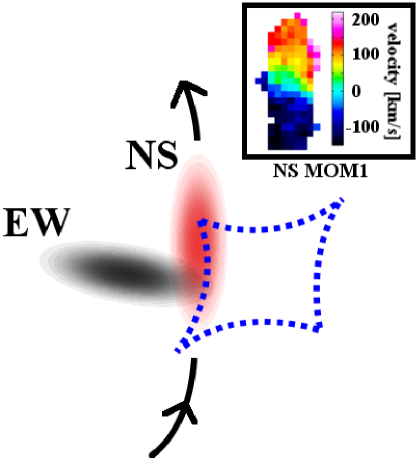
This manuscript reports the latest advances in comprehending the gravitationally-lensed system in HATLAS J142935.3-002836 (also known as H; Messias et al., 2014, M14 henceforth). M14 reported the initial findings on H which appeared as the brightest of an early set of candidates for gravitationally-lensed galaxies in HATLAS (an observed FIR flux at of Jy). It was found that H comprises an edge-on disc galaxy at acting as lens, surrounded by an almost complete Einstein ring with a 3 to 4 knot morphology. Sub-arcsec imaging at near-IR to radio wavelengths enabled reconstruction of the background source to reveal a merging system magnified by an overall factor of and comprising two distinct galaxies at (M14). One galaxy has an East-West orientation dominating the rest-frame optical spectral range (henceforth known as the EW galaxy/component). The other, appearing North-South oriented and with a compact intrinsic half-light radius kpc, dominates the gaseous and dusty content of the system, being the main contributor to the long-wavelength spectral regime flux (henceforth known as the NS galaxy/component). In Dye et al. (2018), the magnification factor of the dust component in NS was revised to be , further highlighting the need for proper magnification lensing analysis incorporating complex morphologies. Figure 1 shows a toy model to help understand the background system. Specifically the inset shows the velocity map of the NS galaxy, where it is clear that its southern region is more blue shifted than the northern one where a peak in velocity dispersion is seen (M14). A more detailed discussion can be found in M14 (specifically, Figures 1 and 8 therein).
In M14, the information available at the time only allowed for the determination of the expected range of molecular gas content. As a result, APEX observations were conducted to observe extra Carbon Monoxide (CO) transitions, thus improving its spectral line energy distribution (SLED), and, together with the already observed [CI] , enable us to assess the gas conditions and content in H1429. Such observations are detailed in Sec. 2, whose results are used together with the lines reported in M14 to pursue a Large Velocity Gradient (LVG) analysis of the CO+[CI] SLED in Sec. 3. The implications of the results presented here are discussed in Sec. 4. Finally, Sec. 5 presents the concluding remarks.
Throughout this paper, the following CDM cosmology is adopted: H0 = 70 km s-1 Mpc-1, , . The Cosmic Microwave Background (CMB) is assumed to expand adiabatically (T, with T; Muller et al., 2013). When stated, the gas mass estimates are corrected by a factor of 1.36 to account for chemical elements heavier than Hydrogen, assuming the latter comprises per cent of the total baryonic matter mass (Croswell, 1996; Carroll & Ostlie, 2006).
2 Observations
Prior to this work, only CO Jup=[2,4,5], [CI] , and CS (10-9) had been observed toward H. The limited number of spectral features, precluded a reliable analysis of the molecular gas content in the system. It was not clear if a two-component CO SLED existed and, given the redshifts of the lens (z=0.218) and sources (z=1.027), there was the possibility that the background CO (5-4) emission measured by ZSPEC at APEX was contaminated by foreground CO (3-2) emission. This work makes use of the previously detected lines, in addition to recent observations of CO Jup=[3,6] transitions to remove the ambiguities mentioned. The new observations are described in the following sub-sections.
2.1 APEX
The instrument suite available at the Atacama Pathfinder EXperiment (APEX) has contributed strongly toward the understanding of H, giving the initial redshift determination of the system and detecting four CO transitions. The Z-SPEC observations targeting the CO transitions J=4-3 and 5-4 were already described in detail in M14. Here, we proceed to describe the more recent SEPIA Band 5 and SHeFI APEX2 observations.
2.1.1 SEPIA Band 5
The CO (3-2) and CS (7-6) transitions were targeted with APEX/SEPIA-Band 5 between 25th May and 5th June 2016 (097.A-0995, P.I. Messias). The lower-side (signal) band was tuned to 170 GHz to cover the two lines of interest, putting the upper-side (image) band at 182 GHz. The observations were conducted under pwv3 mm (ranging from 2.6 to 5.1 mm between 25th May and 1st June, and 1.3 to 1.7 mm on 5th June) using either Jupiter or Mars as calibrators. A standard observing strategy was adopted (wobbler-switching with a 50” amplitude, at a frequency of 0.5 Hz). The total time on source was 5.1 h. The data was reduced with class (a gildas111http://www.iram.fr/IRAMFR/GILDAS task). The rms uncertainty on the final co-added spectrum is 0.3 mK (12 mJy) at a spectral resolution of 100 km/s. The adopted Kelvin to Jansky conversion factor is 38.4 Jy/K (Belitsky et al., 2018).
2.1.2 SHeFI APEX2
The CO (6-5) transition was targeted with APEX/SHeFI-APEX2 on 5th June and between 29th July and 4th August 2016 (097.A-0995, P.I. Messias). The lower-side (signal) band was tuned to 339.8 GHz to cover the line of interest and CS (14-13), putting the upper-side (image) band at 351.8 GHz. The observations were conducted under pwv=0.55–1.4 mm, using IRAS, SW Vir, and SgrB2(N) as calibrators. A standard observing strategy was adopted (wobbler-switching with a 50” amplitude, at a frequency of 0.5 Hz). The total time on source was 4 h. The data was reduced with class (a gildas task). The rms uncertainty on the final co-added spectrum is 0.6 mK (24 mJy) at a spectral resolution of 100 km/s. The adopted Kelvin to Jansky conversion factor is 40.8 Jy/K following the procedure reported in the APEX website222http://www.apex-telescope.org/telescope/efficiency/index.php.
3 Results
3.1 Properties of targeted lines
Altogether, three chemical species (C, CO, CS) and nine transitions have been targeted thus far (M14 and this work). Of these, only CS (7-6) and (14-13), observed by APEX, were not detected, as expected by the depths of these observations. Also, since CO (5-4) has not been spectrally resolved thus far, and because of the possibility of foreground line contamination (Section 1.1), this transition is left out of the analysis. Figures 2 and 3 show the newly targeted CO transitions J=3-2 and 6-5 as observed by SEPIA-Band 5 and SHeFI-APEX2, respectively.
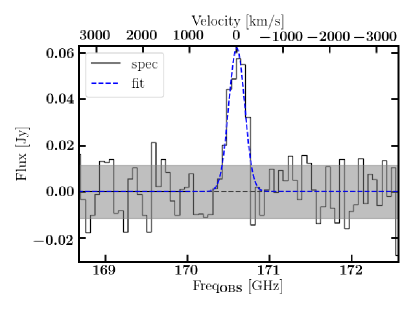
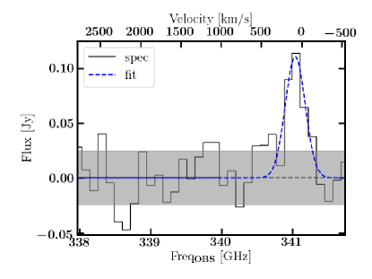
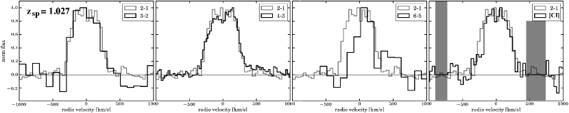
Figure 4 compares the line profiles of the CO transitions detected to date. As already mentioned in M14, the J=2-1 and 4-3 transitions show a double-peak or plateau line-profile. These new APEX observations actually follow this scenario, where the blue-shifted component is stronger at low-J transitions (and almost absent at J=6-5), while the redshifted one is stronger at high-J transitions. This could be a consequence of the red-component being more excited than the blue one as a result of the merger. Henceforth, these blue and red velocity components are referred to as components I and II, respectively.
Interestingly, the additional flux at even higher velocities (km/s, also mentioned in M14; component III henceforth) matches the excess flux seen at km/s in the J=6-5 spectrum. This could be evidence for a shock-induced component, like an outflow. Due to this result, we revisited the HST grism data assessing any possible emission from the arc-like feature external to the Einstein-ring (best seen in HST/WFC3-F110W imaging), in search of evidence of a velocity match between that component and the redshifted one reported here. However, due to the depth of the data and to neighbouring source contamination, no emission is observed. The location and morphology of this feature is addressed later in Section 3.3.
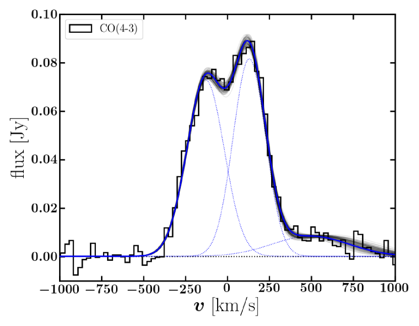
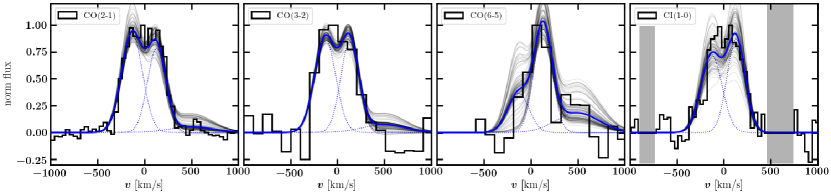
3.2 Spectral Line decomposition
The spectral decomposition of the line-profiles into the three possible spectral components mentioned in the previous section was made in a train-and-fit approach. First, a three-Gaussian fit to the spatially-integrated CO (4-3) spectrum was pursued as a training step by making use of the Python implementation of the affine-invariant ensemble sampler for Markov Chain Monte Carlo (MCMC) proposed by Goodman & Weare (2010), emcee (Foreman-Mackey et al., 2013). This transition was chosen being the one with the highest signal-to-noise ratio allowing for a better line-profile characterisation, and the result can be seen in Figure 5. The training-derived values of the three centroid-velocities were kept fixed while fitting the remainder of the spectrally resolved CO transition spectra. The training-derived Gaussian FWHM values of each component were considered as first guesses. Based on the line-profile discussion in Section 3.1 (see also Figure 4), the flux contribution of each velocity component to each spectrum total flux of a given rotational transition (, where is the velocity-integrated flux of a given velocity component , and the total velocity-integrated flux) had to comply with the following priors: , . Note that the values are those corresponding to the 50th percentile reported from the training step. While fitting the [CI] profile, both the component centroid velocities and FWHMs were fixed to the 50th percentiles reported from the training step. This was done since, although the line-profile shows a plateau, it also reveals a sharp break at 180 km/s and no extra assumptions on the relative component contribution can be adopted like in the other CO transitions333We revisited the data-set to improve the self-calibration step (only in phase) and retrieved the spectrum from the image itself in a common region to CO (4-3) spectrum extraction, not from the model component map as in M14. This resulted in the differences between the [CI] spectrum shown here and in M14.. Due to sky-line contamination, component III is not observable in the [CI] transition.
Figure 6 shows the results of this fitting approach, while Table 1 reports on the velocity-integrated fluxes of each component at each CO and [CI] transitions. The I, II, and III refer to each component ordered by increasing centroid velocity ( km/s, km/s, and km/s as measured in CO J:4-3). Note that components III and I in CO (2-1) and (6-5), respectively, are allowed to be zero, i.e., not to be present, yet the analysis shows that these components are detected at the 3.2 and 1.4 levels ( Jy.km/s and Jy.km/s), respectively.
| Species | Transition | FWHMI | FWHMII | FWHMIII | Facility | ||||
| [Jy km/s] | [Jy km/s] | [km/s] | [Jy km/s] | [km/s] | [Jy km/s] | [km/s] | |||
| CO | 2-1 | ALMA | |||||||
| 3-2 | APEX | ||||||||
| 4-3 | ALMA | ||||||||
| 6-5 | APEX | ||||||||
| [CI] | (263)b | (228)b | … | … | ALMA | ||||
| Note — The central velocities of each component as measured in CO (4-3) are: , , and km/s | |||||||||
| a Values are those retrieved by integrating the observed spectra from -500 km/s to 1000 km/s in CO transitions and to 500 km/s | |||||||||
| in the [CI] transition. | |||||||||
| b The FWHM values for each of the two components in [CI] were fixed to those measured in CO (4-3). | |||||||||
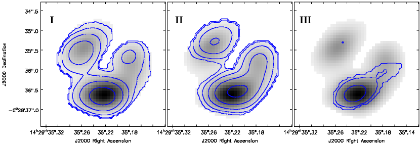
The spectral-spatial decomposition of the three components was also pursued on a pixel-by-pixel basis (i.e., not in the visibility plane). Again, a three-Gaussian fit to the spatially-integrated CO(4-3) spectrum was used as a training step. The training-derived values of the centroid-velocity and Gaussian FWHM of each component were used as reference for each spectrum fit in each cube-pixel, while the relative amplitudes were computed independently for each cube-pixel. Figure 7 shows the result of this spatial-spectral decomposition via the velocity-integrated flux maps (moments-0) of each studied component. The spatial distributions are distinct between the three, hence coming from different regions and this may result in distinct magnifications.
3.3 Differential magnification
Given the extension and multiplicity of the background system, one may wonder whether differential magnification may occur to some degree. In table 3 of M14, the lensing modelling at the time showed a range in the magnification factor between 5 and 11 depending on the spectral band. Since then, new observations have been obtained at much finer spatial-resolution (0.12 arcsec; Dye et al., 2018) tracing the dust emission at rest-frame 696 GHz (430 m). These allowed an improvement of the lens model, which resulted in a revised magnification factor of 241, twice that reported in M14 (10.80.7). Even though the latter was based on slightly lower-frequency data (rest-frame 474 GHz or 632 m), both are tracing cold dust via the Rayleigh-Jeans tail of the spectrum, hence the difference between the two results from the improvement in the lensing model.
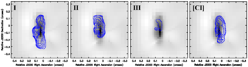
We have thus revised the source reconstruction of the CO (4-3) emission. Specifically, each moment-0 map of the spectral components (Figure 7) was reconstructed separately using the same lens model from Dye et al. (2018), and AutoLens (Nightingale et al., 2018) was used as an independent check of the lens parameters. The best-fit result is seen in Figure 8, where the source areas (A) by counting the number of pixels in the source-plane above are found to be Aarcsec2 (4.1 kpc2), Aarcsec2 (2.6 kpc2), and Aarcsec2 (0.72 kpc2). This new analysis also implies that the current estimate for the dynamical mass and half-light radius of the NS component in the merger is MM⊙ and kpc, which are in agreement with the reported values in M14, where the “isotropic virial estimator” was also assumed: , where , is the CO(4-3) FWHM, and is the half-light radius in units of kpc.
The magnification profiles for each component are displayed in Figure 9. These show how the magnification evolves with cummulative source flux (indicated as fraction of total flux), which is estimated by gradually summing source-plane pixels in decreasing flux order. It is evident that component iii is consistently less magnified than the other two components, which have indistinguishable total magnifications at flux fractions above within errors. The total magnifications are the following: , , and .
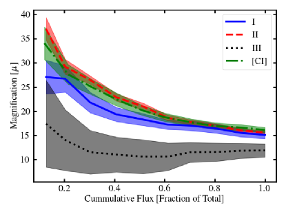
Finally, it is worth assessing the differential magnification between each emission line. The other transition resolved into the ring and knot morphology observed in CO(4-3) is [CI] . The same model from Dye et al. (2018) was applied to the velocity-integrated flux map of [CI]. This time, for the purpose of maximising signal-to-noise ratio, and since the CO(4-3) analysis pointed to no differential magnification between the velocity components I and II, both of these were analysed together (i.e., no spectral deblending was considered). The spatial distribution of the emission at is displayed in Figure 8, comprising an area of Aarcsec2 (3.0 kpc2). The magnification profile is displayed in Figure 9, where it is seen that it follows those observed in CO(4-3) and its total magnification factor is 16.10.6.
As a result, based on the available data, we assume below that the analysis is not affected by differential magnification between velocity-components nor between spectral lines. Specifically, we assume that the velocity components I and II are equally magnified as well as the CO transitions between themselves and with respect to [CI].
3.4 Large Velocity Gradient analysis
In Section 3.3, we make the case that, within the uncertainties, the differences between the two main spectral components I and II are not affected by differential magnification, but rather from different excitation levels (Daddi et al., 2015; Yang et al., 2017; Cañameras et al., 2018). Also, component III is significantly less magnified and its [CI] emission is unconstrained due to sky-line contamination, preventing a proper analysis of its physical conditions. However, given its brightness, it is expected to account for a relatively minor fraction of the molecular gas budget in the system. Nevertheless, follow-up observations are of interest since this feature will likely help understand the current stage of evolution of the merger (e.g., if it is confirmed to be an outflow). As a result, this section will focus on the separate analysis of components I and II alone. We note that it does not consider CO (5-4) since it is not spectrally resolved. In the future, high spatial-resolution imaging will enable proper multi-J spectral and spatial decomposition of the CO emission as it is shown for CO (4-3) in Section 3.3.
As already mentioned, many transitions were detected thus far toward H1429-0028: CO (J, 3, 4, 5, 6), [CI] (), and CS (10-9). The former two species are commonly used to indirectly derive the molecular gas content. While CO is brighter, thus easier to detect, the fine structure system of [CI] is characterised by a simple three-level system easily excited by particle collisions, and is believed to be widespread in giant molecular clouds (Tomassetti et al., 2014, and references therein). The CS molecule is regarded as a high-density gas tracer, hence it could be used as well, but this retrieved poor results (e.g., the predicted CO SLED overestimated the high-J transitions’ fluxes). This may be a result of CS being detected in a very small region in the system, while CO and C are more extended, which could then result in differential magnification (Figure 9), further enhancing the difference.
We adopt the large velocity gradient (LVG) formalism to interpret the CO (J, 3, 4, 6) and [CI] SLED by making use of myRadex444https://github.com/fjdu/myRadex. An escape probability of is assumed in an expanding spherical geometry. The CMB temperature is 5.53 K at . The CO line width was set to 262 and 228 km/s for components I and II, respectively, in accordance to the values in Tab.1. The CO and C abundances relative to H2 (small and ) are both assumed to be , which already implies that a significant fraction of Carbon is locked into CO (Walter et al., 2011), i.e., the CO emission mostly comes from dense molecular regions (e.g., Wolfire et al., 2010; Narayanan et al., 2012). The uncertainty in these abundances is further explored in Section 4.2.
We have adopted different approaches to estimate the gas temperature (T [K]), the molecular number density ( [cm-3]), velocity gradient ( [m/s/pc]), column density (N [cm-2])555Note that the following is assumed: N, and the molecular-gas mass ( [M⊙]), while considering CO and [CI] together. The best-fit value was obtained by finding the minimum -value in a grid of line-intensity values considering conditions ranging , , and , with -steps of 0.1 dex. Maximum Likelihood (ML; e.g., Zhang et al., 2014), Bootstrapping, and MCMC approaches also adopted this same grid and provided the 16th, 50th, and 84th percentiles. While Bootstrapping, a total of 1000 iterations were adopted where, in each one, the observed line-flux values were randomly defined to be around the real observed value following a Gaussian distribution with a standard deviation equal to the estimated flux error. This was adopted in all the above approaches, together with a 5 and 10 per cent error in flux added in quadrature to the instrumental error to account for the uncertainty in the absolute flux scaling in CO (2-1) and the remaining transitions, respectively.
This analysis adopted priors in order to better constrain the results. The H2-mass should not be larger than the dynamical-mass (M, of the dynamical-mass estimate). It is also assumed that the gas is in virial equilibrium or super-virialised, i.e., the velocity gradient is equal or greater than that calculated from the virial equilibrium () as expected from normal to star-burst galaxies (e.g., Papadopoulos & Seaquist, 1999; Zhang et al., 2014).
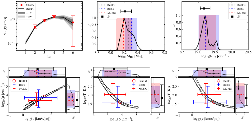
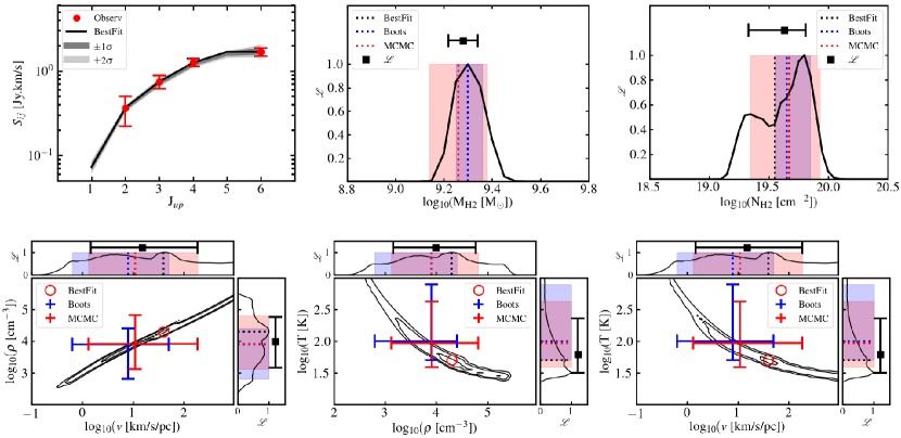
Figures 10 and 11 show the results graphically for the analysis of CO and [CI] for components I and II, respectively, while Table 2 presents the results quantitatively. In the figures, the top left panel shows the observed CO SLED as well as the best-fit (solid black line) and range of acceptable models (shaded grey regions). In the remaining plots, the central panel shows the surface likelihood distribution, with the best-fit value appearing as an open red-circle. Also, the MCMC (red) and Bootstrapping (blue) results appear as error-bars, where their centre indicates the 50th percentile, and the extremes the 16th and 84th percentiles. These ranges are again displayed in the top and side panels as transparent regions (vertical dotted line indicating the 50th percentile). Here, the likelihood distribution for each parameter is shown with a solid line, and its 16th, 50th, and 84th percentiles are displayed with a black error-bar. In the side panels, the vertical black line indicates the best-fit value. For completeness, the predicted [CI] velocity integrated unmagnified fluxes for components I and II together is Jy km/s, which comprises the observed value of .
| Pars.a | Boots. | MCMC | ML | meanb | |
|---|---|---|---|---|---|
| Component I | |||||
| log T | 1.60 | ||||
| log | 3.85 | ||||
| log | 1.50 | ||||
| log N | 19.26 | ||||
| log | -0.94 | ||||
| log M | 9.27 | ||||
| Component II | |||||
| log T | 1.70 | ||||
| log | 4.30 | ||||
| log | 1.60 | ||||
| log N | 19.55 | ||||
| log | -1.00 | ||||
| log M | 9.30 | ||||
| a The parameters in this column are: | |||||
| temperature, log Tlog(T [K]); | |||||
| molecular gas density, log log( [cm-3]); | |||||
| velocity gradient, log log([m/s/pc]); | |||||
| gas column density, log Nlog(N [cm-2]); | |||||
| area filling factor, log log(); | |||||
| and molecular gas mass, log Mlog(M [M⊙]). | |||||
| b This column shows the log-mean between the ML, MCMC, | |||||
| and Bootstrap values. | |||||
4 Discussion
4.1 Gas conditions
From Table 2 and Figures 10 and 11, one can see that temperature, velocity gradient, and gas density are poorly constrained and correlated. As a result, there is no significant difference within the errors in these properties between the two velocity components. The molecular gas column density and mass are better constrained, and, although both velocity components have comparable gas masses (log(M [M⊙])9.26), the column density is higher in II (log(N [cm-2])= versus in I).
Combined, components I and II have (where the errors assume the full range of uncertainty from all methods). For reference, this means that the H2-to-dynamical-mass fraction (i.e., ) in the NS component is per cent.
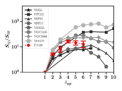
The CO SLED seems to be intermediate between those observed on average in SMGs and QSOs (Fig. 12 and Carilli & Walter, 2013; Oteo et al., 2017b). Nevertheless, compared to the CO transitions luminosity-ratios presented by Carilli & Walter (2013, table 2 therein), the resemblance to SMG-like ratios is strong: , , and versus, respectively, average values of 0.78, 0.54, and 0.46 for SMGs or 0.98, 0.88, and 0.70 for QSOs (Carilli & Walter, 2013). Given the uncertainties and the current lack of evidence supporting the presence of an accreting super-massive black-hole (Timmons et al., 2015; Ma et al., 2018), H1429-0028 is regarded as a DSFG.
Last, but not least, the gas conditions explaining the CO+[CI] SLED predict a CS (10-9) line flux 200 times lower than observed. This indicates that there is either a warm component inducing the population of higher J-levels in the CO-ladder, or the CS (10-9) emission is a result of differential magnification or chemical segregation in the background system. Follow-up observations of higher J-levels or deeper ALMA imaging can address this issue and the incidence of the high-velocity (+500 km/s) component.
4.2 Varying CO and Carbon abundances
4.2.1 Changing alone
The neutral Carbon abundance adopted in the LVG analysis in Section 3.4 is . This value is comparable to the abundance of that was found for a sample of submillimeter galaxies and quasar host galaxies at (Walter et al., 2011), and even in the centres of some local star-forming galaxies (Israel & Baas, 2003; Jiao et al., 2017). However, in the literature, lower values are regularly adopted or reported, down to (Frerking et al., 1989; Sofia et al., 2004; Tomassetti et al., 2014; Israel et al., 2015; Jiao et al., 2017).
As a first assessment, one can assume local thermal equilibrium (LTE) conditions and estimate the neutral carbon mass using the [CI](1-0) line alone (see Section 4.4 in M14 for details on estimating based on [CI]). Considering a carbon excitation temperature of T (Walter et al., 2011) and an observed [CI] luminosity from components I and II together of K km/s pc2, one retrieves . This implies a molecular gas mass of , where and we have explicitly included the carbon abundance as an optional alternative to our adopted value. Within , this estimated value agrees with the one obtained from the LVG analysis. One can see that the estimate will vary linearly with the ratio.
We have also redone the LVG analysis assuming and . This induces an increase in the estimate by a similar factor to which the was reduced by (), just as in the LTE assumption above. In this way, the molecular gas mass in components I and II would increase from to 9.75 and from 9.28 to 9.77, respectively. However, although the best-fit provides acceptable physical values, the peaks of the likelihood distributions and the MCMC posteriors imply very low volume densities cm-3 (even unconstrained in component I within the model grid), and very low velocity gradients unconstrained down to the lowest values in the model grid ().
4.2.2 Assessing a metallicity dependence
Finally, one can assume that both and are proportional to metallicity (e.g., as in Wolfire et al. 2010 or Narayanan et al. 2012), one arrives to the conclusion that , where . The exponent here is assumed to be dependent on , , and the densities of these atoms, which already points to if one assumes that both C and O originate from the same process (stellar activity), and no CO dissociation occurs due to less shielding-effects at lower-metallicity.
As a result, we have ran the LVG analysis assuming and . Here, and are the neutral Carbon and CO abundances, respectively, adopted in Section 3.4, Z is the measured metallicity in (see Section 4.3.1) and Z⊙ is the solar metallicity (8.69; Asplund et al., 2009). This implies and . This approach results in total molecular mass of , which is a factor of higher than the estimate reported in Section 3.4. Again, this factor is comparable to the one was reduced by.
4.2.3 Accounting for the abundance uncertainty
As made clear in the previous sub-sections, the estimate varies proportionally with the assumption. Hence, as a conservative approach, and specifically considering the spread of the order of 40 per cent in the abundances found in the sample studied by Walter et al. (2011), a more realistic error estimate for the molecular gas estimate would be , where the upper error estimate also accounts for the metallicity dependence uncertainty discussed in Section 4.2.2. This implies an H2-to-dynamical-mass fraction in the NS component of per cent.
4.3 CO-to-H2 conversion-factor
The CO/[CI] SLED analysis pursued in Sec. 3.4 (Figs. 10 and 11) implies a velocity-integrated J=1-0 line-flux of mJy km/s, implying a line luminosity of K km/s pc2 (assuming a magnification of , Section 3.3). This implies that the CO-to-H2 conversion-factor in H is M⊙/(K km/s pc, assuming .
4.3.1 Comparison with metallicity-dependent relations
As it has been proposed in the literature (Bolatto et al., 2013, for a review), the CO-to-H2 conversion factor (, ) appears to be dependent on gas-phase metallicity, where CO gradually becomes a poor tracer of H2 with decreasing metallicity.
Using 0.8-1.7 m grism data acquired by HST/WFC3, Timmons et al. (2015) assessed the gas-phase metalicity, 12+log(O/H), for H. Their analysis revealed the AB knot (Figure 1 in M14) as the brightest line emitter in the Einstein ring, resembling the knot flux-ratios seen at long-wavelengths (mm), and in contrast with the rest-frame optical ones. This points to the fact that line emission is dominated by the North-South (NS) oriented component in the background system (Figure 8 in M14) also dominating the long-wavelength spectral range.
Following the linear relation proposed by Sobral et al. (2015) between H[NII] flux ratios and the logarithm of the H[NII] equivalent width, one can use the former to estimate the metallicity based on the N2-index relations proposed by Denicoló et al. (2002) and Pettini & Pagel (2004), giving, respectively, and . Since the N2-index is known to saturate at metallicities close to solar, Pettini & Pagel (2004) proposed the O3N2-index which yields . Assuming a solar metallicity of 8.69 (Asplund et al., 2009), H is observed as a system with a metallicity close to solar (e.g., O3N2 estimate is away).
Following the metallicity- relation proposed by (Genzel et al., 2012, which is based on the N2 calibration by Denicoló et al. 2002), is found to be 5.3 M⊙/(K km/s pc (with an error factor of 1.7)666The reported error factor considers instrumental error alone, and not the scatter of the relation proposed by Genzel et al. (2012).. Based on the theoretical predictions by Wolfire et al. (2010) and Glover & Mac Low (2011) (which Bolatto et al., 2013, show to best explain observations), and the empirical metallicity values just mentioned, the expected is very much Milky-Way-like (M⊙/(K km/s pc). An alternative theoretical approach by Narayanan et al. (2012) predicts a relation between and both metallicity and CO line-intensity. This yields M⊙/(K km/s pc, assuming the O3N2 metallicity index value and the as measured in the source-plane CO(4-3) moment-0 map scaled to the CO(1-0) flux predicted from the SLED analysis.
However, as briefly noted in M14, such high values imply values () comparable or higher than the estimated dynamical mass (MM⊙). As a result, these are deemed not realistic in the case of H.
4.3.2 Comparison with the relation
Since spectral line observations are time-consuming, the statistical approach proposed by Scoville et al. (2016, see also ), where the dust continuum is used as a tracer of molecular-gas, has become increasingly popular, since one can study numerous galaxies in a very inexpensive way. For completeness, the application of this relation to the case of H is reported here. We note however that the relation assumes a constant galactic-like M⊙/(K km/s pc 777Note this value already includes a factor of 1.36 to account for elements heavier than Hydrogen., hence what should actually be compared here is CO (1-0) luminosity. Following Equation 16 in Scoville et al. (2016, Appendix A.6), we assume a power-law index of (M14) instead of 3.8, and erg/(s Hz M⊙). We also consider the mbb_emcee888https://github.com/aconley/mbb_emcee SED fit to mm photometry in M14 to predict the observed flux at rest-frame 850 m, which avoids the need for the Rayleigh-Jeans approximation correction. This implies and K km/s pc2. While the -mass estimate comprises the SLED analysis result, the CO(1-0) luminosity is a factor of lower than the predicted one (see values summarised in Section 4.3). Nevertheless, H is a lensed galaxy and the errors are still relatively large. As a result, for the time being, this predicted-luminosity 1.8 difference ought to be considered as statistically insignificant.
4.4 The different ISM contents in the two background components
To the depth of the current observations, it is observed that the gas and dust emissions are totally dominated by the NS component. Since the 1.28 mm observations are probing the Rayleigh-Jeans tail of the dust continuum, we can use that information as a tracer of the ISM gas in the system (Scoville et al., 2016). Here, we chose to use this property to assess the relative ISM content between the EW and NS components. From Table 2 in M14, it is observed that the total 1.28 mm flux is mJy (all assigned to the NS component), while the observations reached an rms of Jy, meaning a upper-limit of mJy. Based on the latest lensing model, the magnification factors for the NS and EW components are and , respectively 999The adopted magnification factor for this component is that measured at -band, emission which is dominated by the EW component.. As a result, the EW gas and dust content is per cent 101010The uncertainty here takes into account a factor of 2 in uncertainty to account for dust-to-gas ratio variations. of that observed in the NS component (i.e., ). A more direct comparison requires deeper 1 mm dust-continuum data or higher spatial resolution observations of low-J transitions (J), where a less excited CO SLED from the EW component is expected to peak, and NIR spectral observations to assess the dynamic properties of the EW component.
4.5 Comparison with SED fitting analysis
In M14, we adopted a two step approach to retrieve the background emission uncontaminated by the foreground one. We used galfit in the high spatial resolution F110W, , and bands imaging to deblend foreground and background emission. Based on this, we later used MagPhys (adopting the default low- template library; da Cunha et al., 2008) to determine the foreground emission in the remainder low spatial resolution imaging. On top of this, we further corrected the background rest-frame UV/optical emission for foreground obscuration (adopting different scenarios and taking them into account in the photometry error budget) and differential magnification. Nevertheless, Ma et al. (2018) has recently shown that, even after this considered approach, depending on the star-formation history assumed for the template library used for the SED fitting, one can retrieve significantly different conclusions. Also, Zhang et al. (2018) also shows that the initial mass function in sources alike H1429 may be top-heavy, which was not considered in M14 nor Ma et al. (2018). Although these issues affect even unlensed systems, H1429 has also been shown to be comprised by two spatially separated components, one dominating the UV/optical spectral range, the other the FIR-radio one. This goes against the underlying assumption of both MagPhys and CIGALE (Noll et al., 2009) where the stellar and dust components are co-spatial.
As a result, in this manuscript, we avoid any discussion involving conclusions based on the SED fitting done in previous works. Since the molecular and dust content is mostly dominated by the NS component, this work is essentially a description of its properties based on the mm observations reported here and in M14.
5 Conclusions
In this paper, the gravitationally-lensed galaxy merger HATLAS J142935.3-002836 (H1429-0028) at presented in Messias et al. (2014) is characterised in further detail. Specifically, recent APEX observations with SHeFI-APEX2 and the recent SEPIA-Band 5 instrument targeting, respectively, the CO transitions J=6-5 and 3-2, allowed us to assess the ISM gas content in the background system.
Thanks to the recent APEX observations and previous ALMA ones, a continuous coverage of the CO-SLED from Jup=2 to 6 is now available, together with the [CI] transition. We have identified three different velocity components comprising the spectra with velocity centroids at km/s, km/s, and km/s (Sec. 3.2). It is observed that they contribute differently to each transition, but, based on the updated lensing model we find that the two brightest components are equally magnified by a factor of , while the fainter one is magnified by . We also show that the high-velocity component is morphologically much smaller than the others, which seems to agree with its expected higher degree of excitation. Only the two main components I and II were considered in the analysis, since the high velocity one is unconstrained in the [CI] spectrum. See Sec. 3.1, 3.2, and 3.3.
Assuming a large velocity gradient scenario and a combined statistical approach (Maximum Likelihood, Markov Chain Monte Carlo, Bootstrap), the molecular gas content in H is estimated to be , where the error accounts for the uncertainty in neutral Carbon and CO abundances. This amount of gas comprises about per cent of the dynamical mass in the NS component. As a result, at the time of observation, this star-formation event is expected to turn only up to 15 per cent ( upper-limit) of the total (dynamical) mass into stars. No major excitation differences between components I and II are observed, but the column density is apparently higher toward component I. Averaging over the many statistical approaches and over the two main velocity components, the gas temperature, volume density, and velocity-gradient are constrained within a factor of 3 on a galaxy-wide view. These parameters are estimated to be T70 K, , and km/s/pc. The gas column density is constrained within a factor of 1.4 to be . See Sections 3.4 and 4.2.
Compared to galaxy samples in the literature, H is observed to have a DSFG-like CO-SLED (in line with the lack of evidence thus far supporting the presence of AGN; Timmons et al., 2015; Ma et al., 2018) and, based on the predicted CO (1-0) velocity-integrated flux, a CO-to-H2 conversion factor (M⊙/(K km/s pc). See Section 4.1.
The spatially-resolved dust continuum map allows us to have a first assessment of the relative ISM gas content between the two background components. We estimate that the EW component is very gas and dust poor with a content less than per cent of what is observed toward the NS component (i.e., M⊙). See Section 4.4.
Acknowledgements
HM thanks the opportunity given by the ALMA Partnership to work at the Joint ALMA Observatory via its Fellowship programme. HM acknowledges support by FCT via the post-doctoral fellowship SFRH/BPD/97986/2013.
We thank insightful discussion with Paola Di Matteo from the GalMer team while attempting to understand this system by the use of galaxy-merger models.
We thank the comments provided by Asantha Cooray.
NN acknowledges support from Conicyt (PIA ACT172033, Fondecyt 1171506, and BASAL AFB-170002).
ZYZ and IO acknowledges support from the European Research Council in the form of the Advanced Investigator Programme, 321302, cosmicism.
SD is supported by the UK STFC Rutherford Fellowship scheme.
E.I. acknowledges partial support from FONDECYT through grant N∘ 1171710.
D.R. acknowledges support from the National Science Foundation under grant number AST-1614213.
MJM acknowledges the support of the National Science Centre, Poland through the POLONEZ grant 2015/19/P/ST9/04010; this project has received funding from the European Union’s Horizon 2020 research and innovation programme under the Marie Skłodowska-Curie grant agreement No. 665778.
Based on data products from observations made with APEX telescope under programmes IDs C-087.F- 0015B-2011, 087.A-0820, 088.A- 1004, and 097.A-0995.
This paper makes use of the following ALMA data: ADS/JAO.ALMA#2011.0.00476.S. ALMA is a partnership of ESO (representing its member states), NSF (USA) and NINS (Japan), together with NRC (Canada), MOST and ASIAA (Taiwan), and KASI (Republic of Korea), in cooperation with the Republic of Chile. The Joint ALMA Observatory is operated by ESO, AUI/NRAO and NAOJ.
References
- ALMA Partnership et al. (2015) ALMA Partnership, Vlahakis, C., Hunter, T. R., et al. 2015, ApJ, 808, L4
- Asplund et al. (2009) Asplund, M., Grevesse, N., Sauval, A. J., & Scott, P. 2009, ARA&A, 47, 481
- Astropy Collaboration et al. (2013) Astropy Collaboration, Robitaille, T. P., Tollerud, E. J., et al. 2013, A&A, 558, A33
- Belitsky et al. (2018) Belitsky, V., Lapkin, I., Fredrixon, M., et al. 2018, A&A, 612, A23
- Bolatto et al. (2013) Bolatto, A. D., Wolfire, M., & Leroy, A. K. 2013, ARA&A, 51, 207
- Bothwell et al. (2013) Bothwell, M. S., Smail, I., Chapman, S. C., et al. 2013, MNRAS, 429, 3047
- Bothwell et al. (2017) Bothwell, M. S., Aguirre, J. E., Aravena, M., et al. 2017, MNRAS, 466, 2825
- Calanog et al. (2014) Calanog, J. A., Fu, H., Cooray, A., et al. 2014, ApJ, 797, 138
- Cañameras et al. (2018) Cañameras, R., Yang, C., Nesvadba, N. P. H., et al. 2018, A&A, accepted
- Carilli & Walter (2013) Carilli, C. L., & Walter, F. 2013, ARA&A, 51, 105
- Carroll & Ostlie (2006) Carroll, B. W., & Ostlie, D. A. 2006, An introduction to modern astrophysics and cosmology / B. W. Carroll and D. A. Ostlie. 2nd edition. San Francisco: Pearson, Addison-Wesley, ISBN 0-8053-0402-9. 2007, XVI+1278+A32+I31 pp.
- Casey et al. (2014) Casey, C. M., Narayanan, D., & Cooray, A. 2014, Phys. Rep., 541, 45
- Chilingarian et al. (2010) Chilingarian, I. V., Di Matteo, P., Combes, F., Melchior, A.-L., & Semelin, B. 2010, A&A, 518, A61
- Croswell (1996) Croswell, K. 1996, The alchemy of the heavens., by Croswell, K.. Oxford University Press, Oxford (UK), 1996, XII + 340 p., ISBN 0-19-286192-1
- da Cunha et al. (2008) da Cunha, E., Charlot, S., & Elbaz, D. 2008, MNRAS, 388, 1595
- Daddi et al. (2010) Daddi, E., Bournaud, F., Walter, F., et al. 2010, ApJ, 713, 686
- Daddi et al. (2015) Daddi, E., Dannerbauer, H., Liu, D., et al. 2015, A&A, 577, A46
- Danielson et al. (2011) Danielson, A. L. R., Swinbank, A. M., Smail, I., et al. 2011, MNRAS, 410, 1687
- Denicoló et al. (2002) Denicoló, G., Terlevich, R., & Terlevich, E. 2002, MNRAS, 330, 69
- Dye et al. (2014) Dye, S., Negrello, M., Hopwood, R., et al. 2014, MNRAS, 440, 2013
- Dye et al. (2018) Dye, S., Furlanetto, C., Dunne, L., et al. 2018, MNRAS, 476, 4383
- Eales et al. (2010) Eales, S., Dunne, L., Clements, D., et al. 2010, PASP, 122, 499
- Foreman-Mackey et al. (2013) Foreman-Mackey, D., Hogg, D. W., Lang, D., & Goodman, J. 2013, PASP, 125, 306
- Frayer et al. (2011) Frayer, D. T., Harris, A. I., Baker, A. J., et al. 2011, ApJ, 726, L22
- Frerking et al. (1989) Frerking, M. A., Keene, J., Blake, G. A., & Phillips, T. G. 1989, ApJ, 344, 311
- Genzel et al. (2012) Genzel, R., Tacconi, L. J., Combes, F., et al. 2012, ApJ, 746, 69
- Gerhard et al. (2001) Gerhard, O., Kronawitter, A., Saglia, R. P., & Bender, R. 2001, AJ, 121, 1936
- Glover & Mac Low (2011) Glover, S. C. O., & Mac Low, M.-M. 2011, MNRAS, 412, 337
- Glover & Clark (2012) Glover, S. C. O., & Clark, P. C. 2012, MNRAS, 421, 9
- Goodman & Weare (2010) Goodman, J., & Weare, J. 2010, Communications in Applied Mathematics and Computational Science, Vol. 5, No. 1, p. 65-80, 2010, 5, 65
- Harris et al. (2012) Harris, A. I., Baker, A. J., Frayer, D. T., et al. 2012, ApJ, 752, 152
- Hezaveh et al. (2012) Hezaveh, Y. D., Marrone, D. P., & Holder, G. P. 2012, ApJ, 761, 20
- Hughes et al. (1998) Hughes, D. H., Serjeant, S., Dunlop, J., et al. 1998, Nature, 394, 241
- Hughes et al. (2017) Hughes, T. M., Ibar, E., Villanueva, V., et al. 2017, MNRAS, 468, L103
- Hunter (2007) Hunter, j. D. 2007, Computing in Science & Engineering, 9, 90-95
- Israel & Baas (2003) Israel, F. P., & Baas, F. 2003, A&A, 404, 495
- Israel et al. (2015) Israel, F. P., Rosenberg, M. J. F., & van der Werf, P. 2015, A&A, 578, A95
- Jiao et al. (2017) Jiao, Q., Zhao, Y., Zhu, M., et al. 2017, ApJ, 840, L18
- Jones et al. (2001) Jones, E., Oliphant, T. E., Peterson, P., et al. 2001-, http://www.scipy.org/
- Kassin et al. (2006) Kassin, S. A., de Jong, R. S., & Weiner, B. J. 2006, ApJ, 643, 804
- Kennicutt (1998) Kennicutt, R. C., Jr. 1998, ARA&A, 36, 189
- Kennicutt & Evans (2012) Kennicutt, R. C., & Evans, N. J. 2012, ARA&A, 50, 531
- Krumholz (2012) Krumholz, M. R. 2012, ApJ, 759, 9
- Liang et al. (2018) Liang, L., Feldmann, R., Faucher-Giguère, C.-A., et al. 2018, MNRAS, 478, L83
- Liu et al. (2015) Liu, L., Gao, Y., & Greve, T. R. 2015, ApJ, 805, 31
- Lupu et al. (2012) Lupu, R. E., Scott, K. S., Aguirre, J. E., et al. 2012, ApJ, 757, 135
- Ma et al. (2015) Ma, B., Cooray, A., Calanog, J. A., et al. 2015, ApJ, 814, 17
- Ma et al. (2018) Ma, J., Brown, A., Cooray, A., et al. 2018, arXiv:1807.06664
- Messias et al. (2014) Messias, H., Dye, S., Nagar, N., et al. 2014, A&A, 568, A92
- Mirabel & Sanders (1989) Mirabel, I. F., & Sanders, D. B. 1989, ApJ, 340, L53
- Motta et al. (2018) Motta, V., Ibar, E., Verdugo, T., et al. 2018, ApJ, 863, L16
- Muller et al. (2013) Muller, S., Beelen, A., Black, J. H., et al. 2013, A&A, 551, A109
- Narayanan et al. (2012) Narayanan, D., Krumholz, M. R., Ostriker, E. C., & Hernquist, L. 2012, MNRAS, 421, 3127
- Negrello et al. (2010) Negrello, M., Hopwood, R., De Zotti, G., et al. 2010, Science, 330, 800
- Negrello et al. (2017) Negrello, M., Amber, S., Amvrosiadis, A., et al. 2017, MNRAS, 465, 3558
- Nightingale et al. (2018) Nightingale, J. W., Dye, S., & Massey, R. J. 2018, MNRAS, 478, 4738
- Noll et al. (2009) Noll, S., Burgarella, D., Giovannoli, E., et al. 2009, A&A, 507, 1793
- Oliver et al. (2012) Oliver, S. J., Bock, J., Altieri, B., et al. 2012, MNRAS, 424, 1614
- Oteo et al. (2017a) Oteo, I., Zhang, Z., Yang, C., et al. 2017, arXiv:1701.05901
- Oteo et al. (2017b) Oteo, I., Smail, I., Hughes, T., et al. 2017, arXiv:1707.05329
- Papadopoulos & Seaquist (1999) Papadopoulos, P. P., & Seaquist, E. R. 1999, ApJ, 516, 114
- Pérez & Granger (2007) Pérez, F., & Granger, B. E. 2007, Computing in Science & Engineering, 9, 21-29
- Pettini & Pagel (2004) Pettini, M., & Pagel, B. E. J. 2004, MNRAS, 348, L59
- Planck Collaboration et al. (2016) Planck Collaboration, Adam, R., Ade, P. A. R., et al. 2016, A&A, 594, A1
- Riechers et al. (2011) Riechers, D. A., Cooray, A., Omont, A., et al. 2011, ApJ, 733, L12
- Riechers et al. (2013) Riechers, D. A., Bradford, C. M., Clements, D. L., et al. 2013, Nature, 496, 329
- Rosenberg et al. (2015) Rosenberg, M. J. F., van der Werf, P. P., Aalto, S., et al. 2015, ApJ, 801, 72
- Scoville et al. (2016) Scoville, N., Sheth, K., Aussel, H., et al. 2016, ApJ, 820, 83
- Scott et al. (2011) Scott, K. S., Lupu, R. E., Aguirre, J. E., et al. 2011, ApJ, 733, 29
- Serjeant (2012) Serjeant, S. 2012, MNRAS, 424, 2429
- Simpson et al. (2014) Simpson, J. M., Swinbank, A. M., Smail, I., et al. 2014, ApJ, 788, 125
- Smail et al. (1997) Smail, I., Ivison, R. J., & Blain, A. W. 1997, ApJ, 490, L5
- Sobral et al. (2015) Sobral, D., Matthee, J., Best, P. N., et al. 2015, MNRAS, 451, 2303
- Sofia et al. (2004) Sofia, U. J., Lauroesch, J. T., Meyer, D. M., & Cartledge, S. I. B. 2004, ApJ, 605, 272
- Strandet et al. (2016) Strandet, M. L., Weiss, A., Vieira, J. D., et al. 2016, ApJ, 822, 80
- Strandet et al. (2017) Strandet, M. L., Weiß, A., De Breuck, C., et al. 2017, arXiv:1705.07912
- Timmons et al. (2015) Timmons, N., Cooray, A., Nayyeri, H., et al. 2015, ApJ, 805, 140
- Timmons et al. (2016) Timmons, N., Cooray, A., Riechers, D. A., et al. 2016, ApJ, 829, 21
- Toft et al. (2014) Toft, S., Smolčić, V., Magnelli, B., et al. 2014, ApJ, 782, 68
- Tomassetti et al. (2014) Tomassetti, M., Porciani, C., Romano-Díaz, E., Ludlow, A. D., & Papadopoulos, P. P. 2014, MNRAS, 445, L124
- Trujillo et al. (2014) Trujillo, I., Ferré-Mateu, A., Balcells, M., Vazdekis, A., & Sánchez-Blázquez, P. 2014, ApJ, 780, L20
- Van Der Walt et al. (2011) Van Der Walt, S., Colbert, S. C., & Varoquaux, G. 2011, Computing in Science and Engineering 13, 2, 22-30, arXiv:1102.1523
- Vieira et al. (2010) Vieira, J. D., Crawford, T. M., Switzer, E. R., et al. 2010, ApJ, 719, 763
- Vieira et al. (2013) Vieira, J. D., Marrone, D. P., Chapman, S. C., et al. 2013, Nature, 495, 344
- Viero et al. (2014) Viero, M. P., Asboth, V., Roseboom, I. G., et al. 2014, ApJS, 210, 22
- Walter et al. (2011) Walter, F., Weiß, A., Downes, D., Decarli, R., & Henkel, C. 2011, ApJ, 730, 18
- Wardlow et al. (2013) Wardlow, J. L., Cooray, A., De Bernardis, F., et al. 2013, ApJ, 762, 59
- Williamson et al. (2011) Williamson, R., Benson, B. A., High, F. W., et al. 2011, ApJ, 738, 139
- Wolfire et al. (2010) Wolfire, M. G., Hollenbach, D., & McKee, C. F. 2010, ApJ, 716, 1191
- Yang et al. (2017) Yang, C., Omont, A., Beelen, A., et al. 2017, A&A, 608, A144
- Zhang et al. (2014) Zhang, Z.-Y., Henkel, C., Gao, Y., et al. 2014, A&A, 568, A122
- Zhang et al. (2018) Zhang, Z.-Y., Romano, D., Ivison, R. J., Papadopoulos, P. P., & Matteucci, F. 2018, Nature, 558, 260