Decomposition and Modeling
in the Non–Manifold Domain

Abstract

The problem of decomposing non -manifold object has already been studied in solid modeling. However, the few proposed solutions are limited to the problem of decomposing solids described through their boundaries. In this thesis we study the problem of decomposing an arbitrary non-manifold simplicial complex into more regular components. A formal notion of decomposition is developed using combinatorial topology. The proposed decomposition is unique, for a given complex, and is computable for complexes of any dimension. A decomposition algorithm is proposed. This algorithm splits the input complex into a set of connected components in a time proportional to the size of the input. The algorithm splits non-manifold surfaces into manifold components. In three or higher dimensions a decomposition into manifold parts is not always possible. Thus, in higher dimensions, we decompose a non-manifold into a decidable super class of manifolds, that we call, initial-quasi-manifolds. Initial-quasi-manifolds are then carefully characterized and a definition of this class, in term of local topological properties, is established.

We also defined a two-layered data structure, the extended winged data structure. This data structure is a dimension independent data structure conceived to model non-manifolds through their decomposition into initial-quasi-manifoldparts. Our two layered data structure describes the structure of the decomposition and each component.separately. Each decomposition component, in our description, is encoded using an extended version of the winged representation [103]. In the second layer we encode the connectivity structure of the decomposition. We analyze the space requirements of the extended winged data structure and give algorithms to build and navigate it. Finally, we discuss time requirements for the computation of topological relations and show that for surfaces and tetrahedralizations embedded in ${\rm I\kern-1.99997ptR}^{3}$ all topological relations can be extracted in optimal time.

This approach offers a compact, dimension independent, representation for non -manifolds that can be useful whenever the modeled object has few non -manifold singularities.

Dottorato di Ricerca in Informatica
Dipartimento di Informatica e Scienze dell’Informazione
Università degli Studi di Genova

DISI, Univ. di Genova
via Dodecaneso 35
I-16146 Genova, Italy
http://www.disi.unige.it/

Ph.D. Thesis in Computer Science

Submitted by Franco Morando
DISI, Univ. di Genova
morando@disi.unige.it
Date of submission: December 2002
Title: Decomposition and Modeling in the Non -Manifold Domain
Advisor: Enrico Puppo
DISI, Univ. di Genova
puppo@disi.unige.it
Supervisor: Leila De Floriani
DISI, Univ. di Genova
deflo@disi.unige.it
Ai miei genitori, a mia moglie, alle mie figlie

Chapter 1 Introduction

In point set topology a closed manifold object is a subset of the Euclidean space for which the neighborhood of each internal point is locally equivalent to an open ball. An objects that do not fulfill this property at one or more points is what is usually called a non-manifold object. Manifolds deserved and continue to deserve a lot of theoretical investigation from topology. Non-manifolds are less studied and therefore less known objects. The main reason for this is that non-manifold surfaces seems highly unstructured and, therefore, it seems that there is a little chance to find meaningful theoretical results for them. Nevertheless, non-manifolds tend to populate the computer graphics field.

Geometric meshes with polygonal cells are widely used representations of three-dimensional objects. Meshes are ubiquitous within several applicative domains including: CAD, Computer Graphics, virtual reality, scientific data visualization and finite element analysis. As devices for three-dimensional object reconstruction become more and more common [15], non-manifold meshes are likely to become relevant in most applications dealing with three-dimensional objects. For instance, as reported in [55], in a database of 300 meshes used for MPEG-4 core experiments, mainly obtained from the Web, more than half of the models were represented by non-manifold meshes.

The problem of representing and manipulating meshes with non-manifold topology has been studied in solid modeling, mainly by the end of the ’80s (see, e.g., [59, 112, 131]), because of its relevance in CAD/CAM applications. As a consequence, presently, there exist a few non-manifold modelers that represent 3D objects by a mix of wireframe, 2D surfaces and 3D solids.

In non-manifold modelers, non-manifold objects are described through meshes with non-manifold features that are usually encoded directly in an underlying non-manifold data structure. Motivations for using non-manifold modeling and non-manifold data structures have been pointed out by several authors [27, 59, 112, 131]. For instance, Boolean operators are closed in the r-set domain, that is a subset of the non-manifold domain. Sweeping or offset operations may generate parts of different dimensionality, non-manifold topology is required in different product development phases, such as conceptual design, analysis or manufacturing [27, 120].

Non-manifolds support the representation of complex objects made of parts of different dimensionality. Closed surfaces are used to represent three-dimensional parts (enclosed volumes), open surfaces are used to represent two-dimensional parts, lines are used to represent one-dimensional parts, and points are used to represent zero-dimensional parts. The general idea is that some parts of an object must be represented by a lower dimensional object when seen at a sufficiently high level of abstraction. Using non-manifolds, each part of an object can be represented by a geometric complex of the proper dimensionality and characterized by some geometrical and topological shape features. Different parts are then glued together to form a non-manifold complex.

The superior expressive power of non-manifolds is also established in a number of papers on surface simplification (see e.g., [42, 43, 51, 106, 113, 111, 116] ). These papers show that, if we want an intelligible simplified model below a certain size, our simplification must modify the topology of the original mesh and create a non-manifold mesh.

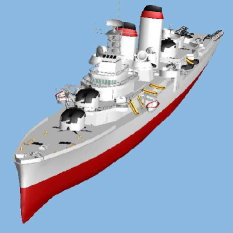
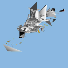
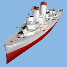
(a) (b) (c)

Figure 1.1: The model in Figure (a) (from [106]) has: 117, distinct, manifold connected components, 167744 triangles and 83799 vertices. Figure (b) shows a simplified model for (a) with 117 connected components, 1154 vertices and 2522 triangles. This model is obtained from (a) by a simplification process that does not modify the (manifold) topology of the original 117 components. Figure (c) shows simplified model for (a) that has only 56 connected components, 1517 triangles, 89 dangling edges and 5 isolated vertices. Model in (c) is a non-manifold version of model (a) and it is a much more intelligible version of (a) and even more compact than (b).

As the figure 1.1 shows, non-manifolds are relevant in simplification but there are other applications where singularities are essential. For instance, one can model the semantic content of an image with an object of mixed dimensionality (e.g., see [71]). Recently non-manifold models become important to provide input to model databases [117]. In this context non-manifolds are used for 3D shape recognition and classification. Indeed, a detailed and non simplified manifold mesh is not structured enough to be used directly for such purposes. A manifold mesh describes the shape of an object as a whole. On the other hand a manifold cannot provide explicit information neither on the subdivision of an object into parts, nor on its morphological features.

Finally, singularities may arise as an undesired side-effects. This happens, for instance, in features extraction from images or in 3D reconstruction. Non-manifold singularities appear also as a byproduct of coarse discretization.

In summary, non-manifold objects are relevant in a number of computer graphic applications. On the other hand, non-manifolds, probably for their apparent unstructured nature, are less studied than manifolds and few characterizations of particular classes of non-manifolds (e.g., r-sets and pseudomanifolds) exist .

1.1 Motivation of the Thesis

As we have seen, in several applicative domains, non-manifold are essential elements. In spite of this fact, non-manifold features are often neither detected nor modeled correctly. We believe that this is a consequence of the fact that a mathematical framework specialized for non-manifoldness is missing. Thus, few approaches to non-manifold modeling exist. Furthermore, they are limited to surfaces [59, 73, 130]. Most of approaches for modeling volumetric data (i.e. tetrahedralizations) are limited to the manifold domain [57, 81].

Another problem is that existing data structures for boundary representations of non-manifold solids [59, 73, 130] are quite space-consuming. This is a consequence of the fact that these modeling approaches implicitly assume that non-manifoldness can occur very often in the model. The resulting data structures are designed to accommodate a singularity everywhere in the modeled object. Thus, storage costs do not scale with the number of non-manifold singularities. On the other hand, much more compact data structures for subdivided 2-manifolds and 3-manifolds do exist [12, 57, 58, 81, 86].

One of the conjectures at the basis of this work is that it could be possible, for a wide class of objects, to provide a more compact representation. This seems possible by modeling a complex through its decomposition. We expected to obtain compact non-manifold modeling by breaking a non-manifold mesh into (possibly) manifold parts and by coding both object parts and assembly separately.

The major problem in taking advantage of this idea lies in the fact that a decomposition of a non-manifold object is not easily available. We believe that the decomposition concept, in general, is not clearly defined, too. Some attempts in this direction are limited to surfaces [37, 46, 55, 56, 114].

In general, all existing proposals develop a decomposition approach that partition a complex into maximal manifold or pseudomanifold connected components. This requirement about maximal components is quite ”natural” since, otherwise the collection of all top simplices in the original complex, each considered as separate component, would be a dumb solution to the decomposition problem. Unfortunately, already for surfaces, it easy to spot examples where several non equivalent, non trivial, decompositions exist (see the example in Figures 1.2 and 1.3). This point is not sufficiently considered in existing approaches (with the notable exception of [114]).

Furthermore, decomposing into manifolds seems to be a theoretically hard problem. As a consequence of some classical results in combinatorial topology [88, 125], there could not exist a decomposition algorithm, for $d\geq 6$, that splits a generic $d$-complex into maximal manifold parts. Such a decomposition problem is actually equivalent to the recognition problem for d-manifolds. This problem is settled for d = 4 [123], it is still an open problem for d = 5, and is known to be unsolvable for $d\geq 6$ [125].

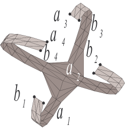
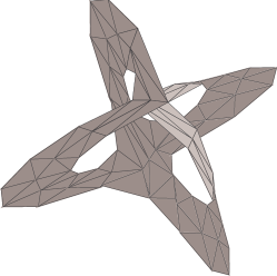
$\mathcal{M}$ (a) $\{a_{1}\approx a_{2}\approx a_{3}\approx a_{4},b_{1}\approx b_{2}\approx b_{3}\approx b_{4}\}$ (b)

Figure 1.2: The Figure 1.2b is a non-pseudomanifold complex obtained from the sheet of Figure 1.2a identifying all segments of the form $a_{i}b_{i}$, i.e. ”applying” equations $\{a_{1}\approx a_{2}\approx a_{3}\approx a_{4},b_{1}\approx b_{2}\approx b_{3}\approx b_{4}\}$. Below each complex in Figures 1.2 and 1.3 is reported the set of equations that tells how to stitch together the sheet $\mathcal{M}$ of Figure 1.2a to build the complex in Figure 1.2b.

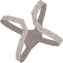
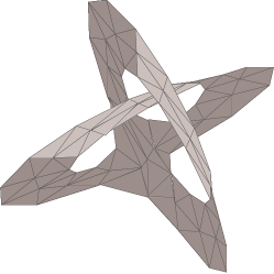
${\{a_{1}{\approx}a_{4},b_{1}{\approx}b_{4},a_{2}{\approx}a_{3},b_{2}{\approx}b_{3}\}}$ (a) ${\{a_{1}{\approx}a_{3},b_{1}{\approx}b_{3},a_{2}{\approx}a_{4},b_{2}{\approx}b_{4}\}}$ (b)

Figure 1.3: The two complexes in Figures 1.3a and 1.3b are two different decompositions of the complex in Figures 1.2b. Both such decompositions consist of one connected component and can be obtained from complex of Figure 1.2b with a minimal number of cuts. Nevertheless, these two optimal decompositions are non homeomorphic. The complex in 1.3a is orientable while the complex in 1.3b is not.

1.2 Goal of the Research

The goal of this thesis is to study the non-manifold domain through decomposition and to develop a non-manifold modeling approach based on this decomposition.

1.2.1 Decomposition

A possible approach for decomposing a non-manifold object is to cut it at those elements (vertices, edges, faces, etc.) where non-manifold singularities occur. The result of such a decomposition should be a collection of singularity-free components. Different components should be linked together at geometric elements where singularities occur. Figure 1.4 depicts an example of a non-manifold object and of one of its possible decompositions.

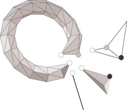
(a) (b)

Figure 1.4: An example (a) of a non-manifold object (described by a three-dimensional simplicial complex made of tetrahedra, triangles and edges) with a dangling edge (A) and a dangling surface formed by two triangles (B) and (C) and its decomposition (b) into ”simpler” components.

However, this definition poses some problems. In two or higher dimensions, we have the above mentioned problem of non-uniqueness of the decomposition (see Figure 1.3). In three or higher dimensions a decomposition into manifold components may need to introduce artificial cuts through certain objects. Figure 1.5a shows an example of such an object: this complex consists of fourteen tetrahedra forming a fan around point $p$. This object is a non-manifold object and point $p$ is a singularity. In order to eliminate the singularity, we necessarily have to cut the object through a manifold face, like the triangle $pqr$ (see Figure 1.5b). This, again, can be done in several ways.

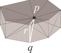
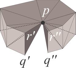
(a) (b)

Figure 1.5: A non-manifold complex made up of of fourteen tetrahedra (a) that can be decomposed into a $3$-manifold (b) by a cut at the non singular (thick) triangle $pqr$.

From examples like this we became aware that a decomposition problem actually exists and started to look for a theoretical solution. Thus, our first goal was to define a notion of decomposition that identifies a unique decomposition even if several decompositions exist. A second issue was to characterize those complexes, like the one of Figure 1.5, that appear as unbreakable. As a consequence, we expected to devise a decomposition algorithm that aims to a unique solution and thus does not need to use any heuristic based optimization process as in [114]. Furthermore, we assumed that this subject could be investigated with a dimension independent approach that should characterize, in a uniform framework, unbreakable $3$-complexes, like the one in Figure 1.5.

To study the decomposition problem we considered a description of non-manifold objects by using abstract simplicial complexes as basic modeling tools. In this way it is possible to study singularities from a purely combinatorial point of view. To this aim we adopted the framework of combinatorial topology [52, 25] as basic mathematical tool. Moreover, we felt that combinatorial models could be the necessary basis for designing effective data structures in solid modeling.

A second issue was the study of the non-manifold domain through the decomposition process. We expect that it could be possible to give a topological characterization of the class of complexes that do not split nicely under decomposition (e.g., the complex of Figure 1.5). In turn this will yield a characterization of the topological properties of the parts produced by the decomposition process.

Finally, in order to define a unique decomposition, we expected that the set of all possible decompositions can be equipped with an order relation of the type ”more decomposed than” such that the set of decompositions will be both a partially ordered set (poset) and a lattice.

1.2.2 Modeling through Decomposition

The first part of this thesis deals with the achievement of previously mentioned goals, i.e. the definition of a dimension independent decomposition algorithm. This is the key enabling factor for the definition of a dimension independent data structure. The second part of this thesis deals with a particular approach to non-manifold modeling through complex decomposition. The basic idea behind this kind of modeling is that the information contained in a solid model comes from two rather independent sources of information that are the structure of the object and the description of its parts. The main goal of this second part of the thesis is to show that a compact representation for non-manifolds can be devised representing structure and parts separately. Parts are usually more regular (i.e. manifolds) and very compact modeling schemes are known for manifolds. Our hope was to show that modeling separately the decomposition structure and its parts would lead to a compact modeling approach. We expected to use less space than approaches that use data structures that can encode non-manifold singularities everywhere. Second we expect that it would have been easy to extend this approach beyond the realm of surfaces to a generic $d$-complex.

We expected to attain these goals using a layered data structure that exploits the outcomes of the decomposition process. In this (foreseen) two-layer data structure the upper layer should be used to encode the structure of the decomposition. On the other hand, the lower level will be used to encode the components of the decomposition. Our initial assumption was that the theoretical results obtained for the decomposition process should support this claim. Furthermore, we expected that, in the decomposition process, just singular (i.e. non-manifold) vertices are duplicated across different components. We will call here, and in all the thesis, these vertices the splitting vertices. The solution seemed to be feasible and especially elegant since the large amount of theoretical work behind the decomposition process allows us to describe non-manifoldness just keeping track of splitting vertices.

Thus, the upper layer actually is a thin layer, just encoding splitting vertices. The hard part of the modeling effort goes in the definition of a data structure that models the components that comes out of our decomposition. As the example of Figure 1.5 shows, in three or higher dimensions there are non-manifold complexes that appear with no assembly structure. They are inherently unbreakable and must be modeled as a single component. Thus, the part, we concentrate our research on, was to match the decomposition outcomes with a modeling approach that models correctly the class of components arising from the decomposition.

Finally, another (self-imposed) commitment was the need for a detailed theoretical analysis of the two layer data structure. In this theoretical analysis our goal was to evaluate both space and time requirements for the proposed data structure. More in particular the goal of this evaluation is detailed in the following checklists.

The checklist for the evaluation of space requirements was basically made up of the following tasks:

• evaluate space necessary to model decomposition components;

• evaluate space requirements when our approach is used to model $2$-manifolds, $3$-manifolds or $d$-manifolds. Compare this with existing approaches for manifolds.

• evaluate space needed to model the connecting structure of the decomposition;

• evaluate space needed to model a non-manifold through its decomposition;

• compare our space requirements with existing approaches for non-manifold modeling;

• evaluate the critical ratio between manifoldness/non-manifoldness that makes our approach more compact than others in non-manifold modeling.

Another evaluation criterion has been time complexity for the extraction of topological relations (e.g., given a vertex, find all top simplices incident into that vertex). The checklist for this evaluation can be divided into two checklists. The first is for the performance of the data structure for components. This checklist is the following:

• evaluate time needed to extract topological relations within a component;

• find under which conditions topological relations can be extracted in a time that is linear with respect to the size of the output;

• evaluate the influence of dimensionality on time complexity and find conditions, if any, in which topological relations cannot be extracted in a time that is linear with respect to the size of the output;

Another checklist is used to evaluate time requirements for the overall two-layered data structure.

• evaluate the time necessary to build the data structure using the outcomes of the decomposition process

• evaluate the time complexity for extracting topological relations in a complex modeled through its decomposition;

• find under which conditions topological relations can be extracted in a time that is linear with respect to the size of the output;

• evaluate the influence of dimensionality on time complexity and find conditions, if any, in which topological relations cannot be extracted in a time that is linear with respect to the size of the output;

• find a relation between the extent of non-manifoldness in the model and the time required to extract topological relations

Finally, we aimed, with the highest priority, at meeting, the following requirements:

• our approach must be more compact than existing approaches for non-manifolds whenever the extent of non-manifold situations is substantially negligible in the combinatorial structure.

• when the extent of the non-manifold situations is negligible, the space requirements must be comparable with that of most common approaches for manifold modeling;

• the extraction of all topological relations should be performed in a time that is linear with respect to the size of the output. This should happen at least in most relevant applicative domains. In particular, extraction in linear time should be guaranteed for non-manifold complexes of dimension two and three emdeddable in the Euclidean space.

1.3 Contribution of the Thesis

This thesis studies, from a mathematical point of view, the problem of decomposing non-manifolds in any arbitrary dimension and presents a dimension independent data structure for non-manifold modeling through complex decomposition.

The work in this thesis starts from a precise, mathematical statement of the decomposition problem. Based on this we give a dimension-independent notion of a standard decomposition. The problem of non-uniqueness of the decomposition is discussed and settled by defining a criterion to select the most general decomposition among all possible options. Existence and uniqueness of this decomposition is mathematically established and an effective algorithm to compute this standard decomposition is proposed. The topological properties of components in our decomposition are studied and precisely characterized.

We have developed a framework for object decomposition that captures, through a systematic approach, all possible decompositions of an input complex $\Omega$. Obviously there are several decompositions of $\Omega$. They are somehow intermediate between $\Omega$ itself, and the complex $\Omega^{\top}$ formed by the totally disconnected collection of all top simplices in $\Omega$. We show that such decompositions form a lattice in which the top is the complex $\Omega^{\top}$ and the bottom is the complex $\Omega$. Transitions between an element and its immediate successors, in this lattice, occurs through stitching a pairs of vertices.

In this lattice we define the standard decomposition of $\Omega$ (denoted by $\nabla\cdot{\Omega}$) as that complex that is obtained from $\Omega^{\top}$ by gluing all top $h$-simplices putting glue just on $(h-1)$-faces that are manifold faces in $\Omega$. We give a mathematical, dimension independent, formulation of intuitive concepts such as: cutting, stitching vertices and gluing faces. Next, we have proven that the standard decomposition is unique and that it is the most general decomposition that can be obtained by cutting the original complex only at non-manifold faces. The connected components of the standard decomposition are thus complexes, like the one of Figure 1.5, from which singularities cannot be eliminated by cutting the complex at manifold faces. We call such a complex an initial-quasi-manifold and we develop a characterization of initial-quasi-manifold complexes in term of local topological properties of the complex.

Initial-Quasi-Manifold complexes are studied and compared with the (few) existing classes of non-manifolds. In particular, we have proven that initial-quasi-manifolds are manifold in dimension two, i.e. the class of 2-initial-quasi-manifoldand 2-manifolds coincide. In dimension $d=3$ or higher d-initial-quasi-manifoldare neither manifolds nor pseudomanifolds i.e. there are initial-quasi-manifoldthat are neither manifolds nor pseudomanifolds. Quasi-manifolds, introduced by [80] are a proper subset of initial-quasi-manifolds, being the set of initial-quasi-manifold that are also pseudomanifolds. A rather counter intuitive finding of this analysis is that there exist non-pseudomanifold $3$-complexes (although not imbeddable in ${\rm I\kern-1.99997ptR}^{3}$) that can be generated by gluing together tetrahedra at triangles where just two tetrahedra glue at time. In other words a non-pseudomanifold adjacency, where three tetrahedra share the same triangular face, can be induced using the (usual) manifold glue (i.e. manifold adjacency) on triangles.

The Initial-Quasi-Manifolds, unlike manifolds, are a decidable class of complexes in any dimension. The standard decomposition itself can be computed in linear time with respect to. the size of the complex $\Omega$. An algorithm to compute the standard decomposition $\nabla\cdot{\Omega}$ is proposed and we have shown that the output of this algorithm is sufficient to build a two-layered data structure for $\Omega$.

Using the results of the decomposition investigation we defined a two-layered data structure that we called the non-manifold winged representation. The non-manifold winged representation represents a non-manifold complex using its standard decomposition. First each component is encoded using an extension of the Winged Representation [103]. We called this extension the extended winged representation. Second, in an upper layer, we encode instructions necessary to stitch initial-quasi-manifold components together.

The non-manifold winged representation is designed to be extremely compact and yet to support retrieval of all topological relations in time linear with respect to the size of the output. This time performance is achieved for $2$-manifolds and for $3$-manifolds embeddable in ${\rm I\kern-1.99997ptR}^{3}$. The proposed data structure is more compact than existing data structures for non-manifold surface modeling. In particular, the proposed data structure is fairly good for objects made up of few nearly manifold parts tied together with (a not-so-large number of) non-manifold joints.

1.4 Thesis Outline

This thesis consists of nine chapters plus an Appendix.

Chapter 2, provides an overview of the state of the art. We review modeling approaches for non-manifolds, for $3$-manifolds and the few dimension-independent modeling approaches. The reviewed modeling approaches are presented in a uniform framework and space requirements for each approach is evaluated. In the second part of this chapter we review papers on non-manifold surface decomposition. Finally, a certain number of classic results in combinatorial topology are presented in order to give an account of the known theoretical problems one can meet when going in higher dimension.

In Chapter 3, we introduce some basic notions from combinatorial topology. In this chapter we added also some results from point set topology. This material, although helpful to understand combinatorial concepts, is actually unnecessary to develop our results. This optional material is reported in this chapter with a starred header (e.g., Definition *).

However, we will use these geometric concepts both in examples and in our quotations from classical handbooks in combinatorial topology (mainly [52, 25]). In other words, we need geometric concepts in order to state classic results in combinatorial topology in their original form.

At the end of this chapter we will introduce, in Section 3.6, the three not-so-standard concepts of: nerve, pasting and quotient space, The nerve concept is needed for the definition of the quotients of an abstract simplicial complex $\Omega^{\prime}$ modulo an equivalence relation $R$ (denoted by $\Omega^{\prime}/R$). Quotients, in turn, are crucial in the definition of the decomposition concept that will come in Chapter 5.

In Chapter 4, we first present the relation between abstract simplicial maps and quotients. We show that the set of all quotients of a given abstract simplicial complex $\Omega^{\prime}$ form a lattice that we called the quotient lattice. The quotient lattice is isomorphic to a well known lattice $\Pi_{n}$ called the partition lattice. Mathematical properties of this lattice are given in Appendix Athat gives a short introduction to the notions from Lattice Theory needed in this thesis. However, in the first part of this chapter, relevant properties of lattices are summarized and restated, in an intuitive form, using a language closer to the subject of this thesis.

Lattices, in the context of this thesis, will be used as the structure in which we order the decompositions of a given complex (we anticipate that decompositions are a sublattice of the quotient lattice that will be is introduced in Chapter 5). There is a clear benefit from organizing decompositions into a lattice. In fact, in this way we grant a least upper bound for any arbitrary set of decompositions. This will be a key issue to define a unique decomposition.

Another key idea in the development of this thesis is the fact that we can manipulate quotients $\Omega^{\prime}/R$ using the set of equations $E$ that defines $R$. In particular we are interested in the fact that some topological properties of a quotient $\Omega/E$ can be restated in terms of syntactic properties of the set $E$. The manipulation of these syntactic objects give us a useful tool to treat topological problems. Since these equations identify two vertices together, we will call them stitching equations. By the end of this chapter, we therefore introduce stitching equations and give the relation between a set of equations $E$ and the quotient lattice.

In Chapter 5, we define the conditions that make $\Omega^{\prime}$ a decomposition of the complex $\Omega$ obtained as the quotient $\Omega^{\prime}/E$. Intuitively, a complex $\Omega^{\prime}$ is a decomposition of $\Omega$ if we can obtain $\Omega$ pasting together pieces of $\Omega^{\prime}$. Furthermore, we expect that nothing shrinks passing from $\Omega^{\prime}$ to $\Omega$. Following this idea, in this chapter, we define the notion of decomposition and define a sublattice of a specific quotient lattice that we called the decomposition lattice. This lattice contains an isomorphic copy for any decomposition of a given complex $\Omega$. On top of the decomposition lattice we have the totally exploded version $\Omega^{\top}$ of $\Omega$. This is the complex consisting of all top simplices in $\Omega$, each one considered as a distinct connected component. At the bottom of the decomposition lattice we have (an isomorphic copy of) the complex $\Omega$. We can walk on the decomposition lattice from $\Omega^{\top}$ to $\Omega$ adding equations whose basic effect is to stitch together two Vertices that belongs to two distinct simplices.

In Chapter 6, we present a more abstract view of the decomposition lattice. This view brings us closer to the solution of the decomposition problem. In the previous chapter we have studied the decomposition lattice for a complex $\Omega$. We have seen that we can walk on the decomposition lattice adding equations. Each equation has the effect of stitching together two Vertices that belongs to two distinct simplices. This view of the decomposition lattice is too fine-grained to be useful in this context. In this chapter we take a different look to the decomposition lattice. We imagine that we do not have the option to stitch just two vertices at time but we are forced to glue together two top simplices $\theta_{1}$ and $\theta_{2}$ by gluing together all Vertices that $\theta_{1}$ and $\theta_{2}$ have in common in $\Omega$. We will call this move a simplex gluing instruction. Obviously, stitching equations provides a more, fine grained, view of the decomposition lattice. In turn a simplex gluing instruction is, basically, a macro expression for a set of stitching equations.

Thus, in this chapter, we introduce simplex gluing instructions and define the subset of decompositions generated by a set of simplex gluing instructions ${\mathcal{E}}$ (usually denoted by $\Omega^{\top}/{\mathcal{E}}$). A discussion on the structure of the set of decompositions $\Omega^{\top}/{\mathcal{E}}$ closes this chapter. In particular we show that not all decomposition can be generated as a quotient of the form $\Omega^{\top}/{\mathcal{E}}$. Furthermore we show that the set of decompositions of the form $\Omega^{\top}/{\mathcal{E}}$ is not a sublattice of the quotient lattice. Nevertheless, the (fewer) complexes of the form $\Omega^{\top}/{\mathcal{E}}$ are sufficient to treat the decomposition problem. This is a consequence of two fundamental lemmas stated at the beginning of Chapter 8.

In Chapter 7, we study topological properties of the decomposition $\Omega^{\top}/{{\mathcal{E}}}$ studying the syntactic properties of the set $\mathcal{E}$. It is possible to relate the topological properties of $\Omega^{\top}/{{\mathcal{E}}}$ with syntactic properties of the set of gluing instruction ${\mathcal{E}}$. We first consider the usual topological properties defined in Chapter 3 such as regularity, connectivity, pseudomanifoldness and manifoldness.

Next we will consider Quasi-manifolds [80] and a superset of quasi-manifolds we called Initial-Quasi-Manifolds. In this chapter quasi-manifolds are defined in terms of syntactical properties of the generating set of simplex gluing instructions ${\mathcal{E}}$. This definition is proven to be equivalent to the definition given by [80].

Then initial-quasi-manifolds are defined in term of syntactical properties of the generating set ${\mathcal{E}}$, too. Next we prove that initial-quasi-manifolds can be defined in terms of local properties each vertex must have. Indeed we have found that, in an initial-quasi-manifold, the star of each vertex has a constant peculiar structure. In fact, every couple of top d-simplices in a star must be connected with a path of d-simplices, each linked to the other via a (d-1)-manifold (non singular) joint.

This local property is sufficient to prove that initial-quasi-manifold d-complexes are a proper superset of d-manifolds for $d\geq 3$. They coincide with manifolds for d = 2. They are a decidable set of d-complexes for any d. Finally we give an example of an initial-quasi-manifold tetrahedralization that is not pseudomanifold. Such a tetrahedralization, however, cannot be embedded in ${\rm I\kern-1.99997ptR}^{3}$ .

In Chapter 8, we first prove two results that enables us to use just simplex gluing instructions in order to treat the decomposition problem. We prove that sets of simplex gluing instructions are sufficient to label every path from any decomposition $\Omega/{\approx}$ down to $\Omega$. Thus we restrict our attention to transformations induced by sets of simplex gluing instructions ${\mathcal{E}}$ and study the relation between syntactic properties of the set ${\mathcal{E}}$ and topological properties of the transformation from $\Omega^{\prime}$ to $\Omega^{\prime}/{\mathcal{E}}$.

Next we define the class of decompositions we are interested in. In particular we are interested in decompositions that split only at non manifold simplices. We will introduce in this chapter the class of ”interesting” decompositions that we called essential decompositions. Then, we define the standard decomposition as the the least upper bound of the set of essential decompositions. Due to lattice structure, this complex exists and is unique. We prove that such a least upper bound is still an essential decomposition. Several properties of the standard decomposition are given, then. In particular, we prove that the connected components of the standard decomposition are initial-quasi-manifolds.

Next, we present an algorithm that transforms a complex into its standard decomposition by a sequence of local operations modifying just simplices which are incident at a vertex. Each local operation is computed using local information about the star of the vertex (i.e., the set of simplices incident to a vertex). Finally we prove that this computation can be done in $O(t\log{t})$, where $t$ is the number of top simplices in the original complex.

In Chapter 9, we define a two layer data structure, we called the non-manifold winged representation. The non-manifold winged representation represents a non-manifold complex using its decomposition.

Each component is encoded using an extension of the winged representation [103]. This extension, that we called the extended winged representation, is carefully presented and its space requirement are assessed. We give algorithms to construct the extended winged data structure using the results of the decomposition process. Next we develop algorithms to extract topological relations in a single component. The complexity of these operations is then analyzed.

In a second step, we define a data structures that encodes the information necessary to stitch components together. This completes the definition of the non-manifold winged data structure. Algorithms to build this data structure are proposed and their time complexity is evaluated. Next, we develop algorithms to extract topological relations in the non-manifold complex. Finally, space requirements of the non-manifold winged  representation are compared with space requirements of other modeling approaches. The conditions that make this structure more suitable than others are discussed.

In Chapter 10 we briefly summarize the results the results of this thesis.open problems.

In Appendix A, we resume basic notions of Lattice Theory and introduce the partition lattice. In Appendix B, we describe the (rather tedious) details of a space optimization for the Extended Winged Data Structure. In Appendix C, we describe a Prolog program that checks the correctness of Example 7.4.2.

Chapter 2 State of the Art

2.1 Introduction

In this thesis we develop a decomposition procedure for a generic simplicial complex. This decomposition procedure cuts the simplicial complexes only at non-manifold singularities. This decomposition is used to build a two layer data structure. In the lower layer we represent decomposition components. In the upper layer we tie together decomposition components. Whenever the decomposed complex is a $2$-complex we have that decomposition components are manifold surfaces. Thus, this two layer approach, gives a data structure whose storage requirement  might be similar to the storage requirements of standard data structures for manifold modeling. This could happen whenever the degree of non-manifoldness is low. The storage requirement then scales up with the degree of non-manifoldness in the decomposed complex.

We found that the subject of this thesis, with a careful choice of the theoretical framework, can be developed with a dimension independent formulation and thus we developed a dimension independent approach.

Existing related literature for this kind of study is surely the literature on manifold and non-manifold modeling. For this reason, in the first part of this chapter, we review modeling approaches for manifold surfaces, for $3$-manifolds, for non-manifolds and the few dimension-independent modeling approaches. The reviewed modeling approaches are presented in a uniform framework and space requirements for each approach is evaluated. In the second part of this chapter we review papers on non-manifold decomposition. Finally, a certain number of classic results in combinatorial topology are presented in order to give an account of the known theoretical problems one can meet in a dimension independent formulation.

This chapter is organized as follows. In Section 2.2, we discuss a basic problem in the relation between approaches for manifold and non-manifold modeling then we revise modeling approaches for manifold surfaces (Section 2.2.1) and for $3$-manifolds (Section 2.2.2). Since we are developing a dimension independent approach, in Section 2.2.3 we insert a review of dimension independent modeling approaches. Next we revise approaches to model cellular subdivisions of non-manifolds (Section 2.2.4). This analysis shows that classic approaches for non-manifold modeling are space inefficient when compared with approaches for manifold modeling.

Next, in Section 2.3, we review papers on decomposition of non-manifold models. Finally, in Section 2.4, we give a rationale for the purely combinatorial framework we developed in this thesis and show that this is necessary if one wants to develop a dimension independent study of decompositions.

2.2 Manifold and non-manifold Modeling

None of the existing modeling approaches for non-manifolds is completely satisfactory. The few approaches that can represent the full domain of non-manifold cellular subdivision of non-manifolds (e.g. Weiler’s Radial Edge [130]) are definitely space inefficient over the manifold domain. The classical data structures for manifold surfaces [12, 58, 98] outperform existing data structures for non-manifolds when the latter are used to model manifolds. This is shown, for instance, by the quantitative analysis developed in [73] where several non-manifold modeling schemes are compared with the two classical data structures for boundary representation of manifold objects. i.e. the Winged–Edge (WE) [12] and the Half Edge [86] (see also [78] for another comparison). Some of the results of comparisons in [73] are summarized in Table 2.1:

Modeling Data Structure		Ratio to WE	Representation Domain
Winged Edge		1	cellular 2-manifolds
1	Radial Edge	4.4	cellular 2-complexes
2	Partial Edge	2.1	cellular 2-complexes
3	Half Edge	1.2	cellular 2-manifolds

Table 2.1: Storage costs normalized with respect to winged-edge storage requirements. Data are from Table 4 in [73]

The analysis in [73] shows that the radial–edge data structure encodes manifold surfaces taking more than four times the space required by the winged–edge.

All data structures for non-manifold modeling have high storage requirements if compared with data structures for manifold modeling. None of the classic data structures for non-manifold modeling have storage requirements that scales with the degree of non-manifoldness in the modeled object. In other words these data structures seems extremely space consuming when they are used to encode manifolds or ”nearly” manifold complexes. This situation, far from being satisfactory, is one of the starting points of this thesis. To fully understand this problem, in Sections 2.2.1 and 2.2.2 we review classical results for manifold modeling. This will provide a benchmark against which we will compare the data structure for modeling the decomposition components we will describe in Section 9.4.

In section 2.2.3 we present four dimension–independent modeling approaches: the cell-tuple [22], the selective geometric complexes [112], the n-G-maps [78] and the winged representation [103]. These provides another set of benchmarks for the data structure designed in this thesis. Furthermore, at least for n-G-maps, some results in this thesis, mainly Property 7.5 can be quite useful in the study of this modeling approaches, while the results in Chapter 9 builds upon an extended version of the Winged Representation [14] and extends it to a dimension independent approach for the non-manifold domain.

In section 2.2.4 we present three modeling approaches that can model cellular subdivisions of non-manifolds realizable in ${\rm I\kern-1.99997ptR}^{3}$. These approaches are reviewed and presented stressing the fact that they all can be understood as small variations around the original scheme presented in the radial-edge data structure. These provides a set of benchmarks for storage requirements against which we will compare our data structure.

In section 2.5 we will resume the shortcomings of this review and discuss the relation of the reviewed material with the results of this thesis.

2.2.1 Data structure for encoding cellular decompositions of manifold surfaces

In this section we review major approaches to represent $2$-manifolds. We start presenting classic data structure for $2$-manifolds (Winged–Edge [12], DCEL [98], Half-Edge [86, 129]). Next we analyze structures based on the Incidence Graph [53, 136]. In the following sections we will present data structures for $3$-manifolds (the Facet Edge [57] and the Handle-Face [81] data structures).

For each data structure, we will give an expression for space requirements with respect to  the number of geometric entities in the model. To this aim, in the following, we will denote with $v$ the number of vertices, with $e$ the number of edges and with with $f$ the number of top faces. Similarly, we will use pairs of letters $V$,$E$,$F$ (e.g. VE) to denote relations between elements of the model. We will say that element $x$ of type $X$ and element $y$ of type $Y$ are in $XY$ relation if one is face of the other. If $x_{1}$ and $x_{2}$ are both of the same dimension (i.e. they are of type $X$), and they share a proper face of maximun dimension, then we will say that they are in the $XX$ relation. Thus two faces are in a $FF$ relation if they share an edge. Two egdes are in a $EE$ relation if they share a vertex. Any $XX$ relation is called an adjacency relation while any $XY$ relation, for $X\neq Y$ is called an incidence relation. In general, we will call the $XY$ and the $XX$ relations topological relations. Finally, we will denote with $XY^{*}$ a function that is a subset of the $XY$ relation. Thus the $VE^{*}$ relation gives an edge incident into a given vertex.

We will call the extraction of an $XY$ relation the retrieval of all $Y$ elements that are in an $XY$ relation with a given $X$ element $x$. Thus, for instance, to extract the $VE$ relation we have to find all the edges that are incident into a given vertex $v$. All data structures listed in this section supports the extraction of all topological relations in a time that is linear with respect to  the size of the output.

The winged–edge Data Structure

The winged­-edge data structure [12] represents each edge of a manifold surface using eight references that points eight cells that are incident to an edge $e$. With reference to Figure 2.1 we have that the eight references relative to the thick edge $e$ are: two references (PVT, NVT) for incident vertices (encoding the EV relation), two references (PFACE, NFACE) for incident faces (encoding the EF relation) and four references (PCW, PCCW, NCW and NCCW) to the incident edges that share with $e$ the same faces and the same vertices. These four references represents a subset of the EE relation.

For a given edge we choose arbitrarily the first extreme vertex PVT and the second extreme vertex NVT thus assigning an orientation to $e$ from PVT to NVT. Face PFACE is the face on the left of someone traveling on the oriented edge standing outside of the surface. A simple convention is at the basis of names for the four references PCW, PCCW, NCW and NCCW. We have that in the above names, CW stands for clockwise, CCW stands for counter-clockwise, N stands for next and P stands for previous. We judge clockwise and counter-clockwise rotations by standing outside the surface. Note that this definition implies that we assume we are modeling an orientable surface. Thus the reference PCW, stored for a certain edge $e$, references the previous edge, in clockwise order, around the source vertex PVT. The four edges PCW, PCCW, NCW and NCCW are the so called wings of the thick oriented edge $e$ in Figure 2.1.

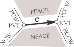
Figure 2.1: A geometric realization of an adge in a surface modeled by a winged–edge data structure. Edges and vertices are labeled with references relative to the thick oriented edge $e$

It can be proven that this data structure models orientable 2­-manifolds subdivided into cell complexes [129]. To extract all topological relations we need to introduce a reference to an incident edge for both vertices and faces (i.e., the $VE^{*}$ and the $FE^{*}$ relation). If we want to retrieve all edges around a face in a given, clockwise (CW) or counterclockwise (CCW), orientation we must check that the edge we are considering has an orientation coherent with the given orientation. This can be checked by a pair of lookup into PFACE and NFACE. These lookups must be repeated for each extracted edge around a face $f$. A similar remark holds for the problem of retrieving all edges around a vertex in a given (clockwise or counterclockwise) orientation. In this case a double lookup to PVT and NVT is needed for each extracted edge.

A double lookup may also be used if we want to extend the WE to a non-orientable surface. If the modeled surface might be non orientable then we cannot assume that the pair of wings incident at PVT (NVT) are labeled as PCW and NCW (PCCW and NCCW) using a counter-clockwise rotation order judged standing outside the surface. For a non orientable surface labels PCW and NCW (PCCW and NCCW) will be assigned using some rotational order around PVT (NVT). The only constraint is that PCW,edge $e$ and PCCW must bound face PFACE and NCW,$e$,NCCW must bound NFACE. When, stating from $e$, we extract a new edge $e\prime$, a first double lookup is needed to find the orientation of $e\prime$. This first lookup will decide whether the wertex $v$, shared by $e$ and $e\prime$, is either $e\prime.PVT$ or $e\prime.NVT$. A second double lookup into the pair of wings incident to the vertex $v$ (recall $v$ is shared by $e$ and $e\prime$), will decide whether $e$ and $e\prime$ use coherent rotational orientation for ordering wings around $v$.

Taking into account the storage requirement of $VE^{*}$ and $FE^{*}$ we have that the storage requirement for this data structure is of $8e+v+f$. It is easy to see that pointers PCW, PCCW, NCW and NCCW organize edges around a vertex into a doubly–linked circular list. Therefore all topological relations can be computed in optimal time. Variants are possible where either vertices (PVT,NVT) or the facets (PFACE,NFACE) can be omitted losing only some of the traversal capabilities.

The quad–edge Data Structure

The quad-edge [58] use the same data structure of the winged–edge but organize the four edge pointers (PCW, PCCW, NCW and NCCW) in a different way. We reported these four pointers for an edge $e$ in Figure 2.2.

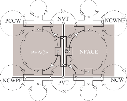
Figure 2.2: A geometric realization of an adge in a surface modeled by a quad–edge data structure. Local clockwise orientation is assumed. Edges and vertices are labeled with references relative to the thick oriented edge $e$

The two data structures differ in the way they define the references they use. First we have that PVT, NVT and PFACE and NFACE are defined as, respectively, the two incident vertices and the two incident faces to edge $e$ (thick in Figure 2.2). To explain the names of references we first assume that there exist a local coherent orientation around vertices and for loops delimiting faces. In Figure 2.2 a CW orientation is chosen. This orientation induces a cyclic ordering of edges around each vertex. References NPVT and NNVT store the next vertex, after $e$ in the ciclic ordering of edges respectively around vertex PVT and NVT. Similarly, references NPF and NNF store the next vertex, after $e$ in the ciclic ordering of edges respectively around face PFACE and NFACE. The definition of the quad–edge data structure do not assume the total orientation of the surface to be encoded. Note that if we reverse the local orientation we will store the same four reference in a different order. It can be proved that with a pair of look-ups we can decide if the orientation of each edge among NPVT, NNVT, NPF and NVF is the same of orientation of $e$ or not. Thus, this data structure can encode non–orientable surfaces and has the same storage requirements of the winged-edge.

In the following we will analyze more compact alternatives to the winged–edge based on the deletion of two of the ”wings”. However, if one wants to support situations where curved edges and faces with one or two edges are allowed, then all four edge pointers must remain. Otherwise, the traversal around a vertex or around a facet is no longer uniquely defined [129]. We start with a winged-­edge data structure where the wings PCCW and NCCW are omitted. This is the so called Doubly Connected Edge List (DCEL).

The DCEL Data Structure

The DCEL (Doubly Connected Edge List) data structure [98] can represent orientable surfaces and assumes that all edges receive an orientation. Then the DCEL represents each oriented edge of the surface using six references: two references (PVT, NVT) for incident vertices (i.e. the EV relation), two references (PFACE, NFACE) for incident faces (i.e. the EF relation) and the two references (PCW and NCCW) as defined in section 2.2.1.

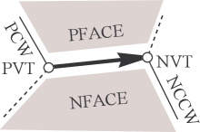
Figure 2.3: A geometric realization of an edge in a surface modeled by a DCEL data structure.

These two references represents a portion of the EE relation. It is easy to see that edges around a vertex are linked in a simply linked circular list. The next element in this list is the next edge around a vertex in CCW order. With these relations we can retrieve all topological relation in optimal time. The only limitation is that the $FE$ and the $VE$ relations are extracted in a particular order i.e., the edges around a vertex are returned in CCW order and edges around a face are returned in CW order.

Again, to extract all topological relations we need to model both vertices and oriented faces with a reference to an incident edge (i.e. $VE^{*}$ and $FE^{*}$ relation). Taking into account the $VE^{*}$ and the $TE^{*}$ relations the storage requirement for this data structure is equal to $6e+v+f$.

The Half-Edge Data Structure

With the term Half–Edge we denote a number of data structures that split the winged-edge representation i.e., the eight references: PVT, NVT, PFACE, NFACE, PCW, PCCW, NCW and NCCW into two similar nodes, called half-edges. Total information is preserved because each half-edge points to the other half using a mutual reference called OTHERH. Two options are described in [129] as the face-edge data structure (FES) and the vertex-edge data structure (VES). The FES keeps in each half-edge (see Figure 2.4b) the four references to NFACE, PVT, NCW, NCCW from the winged–edge data structure (see Figure 2.4a). The VES keeps the four references to PFACE, PVT, NCW, PCW (see Figure 2.4c) in the half-edge description.

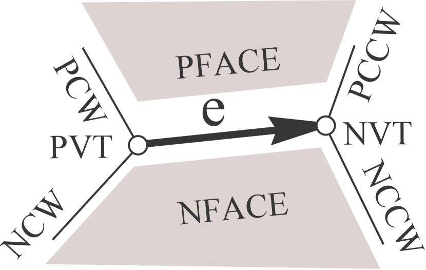
(a)

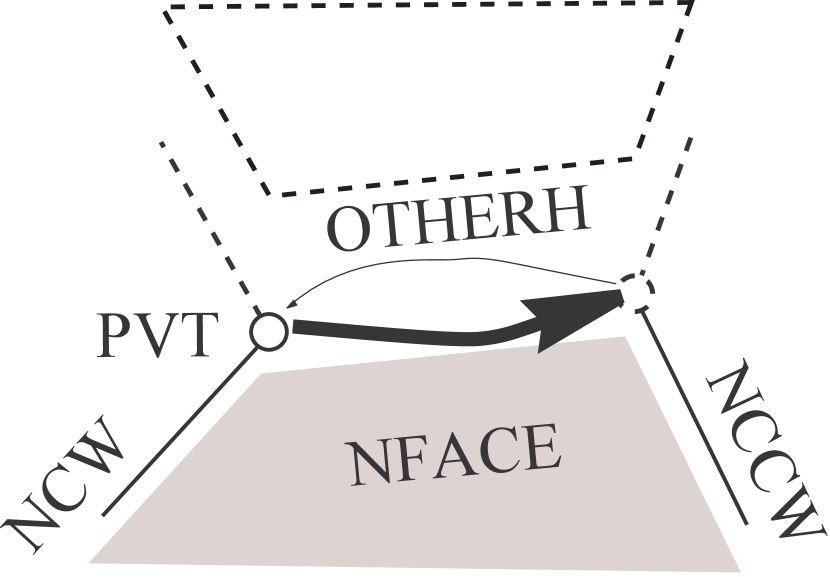
(b)

(c)

Figure 2.4: A geometric realization of an edge in a surface modeled by a winged–edge (a) and one (the thick one) of the two possible half-edges in the face–edge structure (FES) (b) and in the vertex–edge VES structure (c)

It is easy to see that these references link all edges incident to a vertex in a doubly–linked list. To extract all topological relations we need to model both vertices and faces with a reference to an incident half-edge (i.e. $VE^{*}$ and $FE^{*}$ relation). Thus the storage requirement for these two variant of the half-edge is equal to $10e+f+v$.

By storing the two additional pointers in the half–edge data structure we can extract edges bounding a given face either in CW and in CCW order without any need of doing a double lookup into PFACE and NFACE as needed with the winged-edge structure. For this reason, the reference to NFACE in the FES and the reference to PFACE in the VES half-edge are unnecessary whenever one is not interested in the EF relation. With a similar argument one can delete the PVT references if the EV relation is not needed. Next, one can exploit the ideas used in the DCEL approach and reduce the storage requirement by deleting a pointer in each half-edge [67]. For the FES one just need to keep, in the half-edge, the three references to NFACE, PVT, NCCW (see Figure 2.5a). For the VES one just need to keep in the half-edge the three references to PFACE, PVT, PCW (see Figure 2.5b).

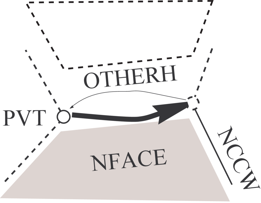
(a)

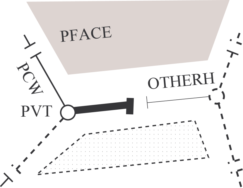
(b)

Figure 2.5: A geometric realization of an edge in a surface modeled by a reduced half-edges following the FE-structure half-edge (a) and the VE-structure half-edge (b)

The storage requirement for these schemes is therefore equal to $8e+v+f$. In this way, the edges around a vertex are linked in a simply linked circular list. With these schemes $FE$ and $VE$ relations are extracted in a fixed order. In particular the edges around a vertex are returned in CCW order and the edges around a face are returned in CW order. Note that again we have no need to reference to PFACE or NFACE or PVT to extract VE and FE relations. If we take this option and delete these references we obtain an storage requirement equal to $4e+v+f$.

Comparison

In conclusion we have five data structures: the winged–edge (WE), the quad–edge, the DCEL and the FES and VES variants to the half-edge (HE) data structures. These data structures offer a range of solutions for the representation of a manifold surface with different memory requirements. With small differences they all supports optimal extraction of topological relations. The different options are summarized in Table 2.2.

Space		Relations Modeled
1	$f$	${\rm FE}^{*}$ relation
2	$v$	${\rm VE}^{*}$ relation
3	$2e$	EV relation
4	$2e$	EF relation
5	$2e$	VE/$e$ and FE/$e$ relation in fixed order (reduced HE)
6	$4e$	VE/$e$ and EV relation in fixed order with double lookup (DCEL)
7	$4e$	FE/$e$ and EF relation in fixed order with double lookup (DCEL)
8	$6e$	EV, EF, VE/$e$ and FE/$e$ relation in fixed order with double lookup (DCEL)
9	$6e$	VE/$e$ and FE/$e$ relation in CW and CCW order (HE)
10	$6e$	VE/$e$ and EV relation in CW and CCW order with double lookup (WE)
11	$6e$	FE/$e$ and EF relation in CW and CCW order with double lookup (WE)
12	$8e$	EV, EF, VE/$e$ and FE/$e$ relation as in $10$ and $11$ (WE)
$f+v+6e$		DCEL (FE and VE in fixed order) (1+2+8)
$f+v+8e$		WE (FE and VE in CW and CCW order with double lookup) (1+2+12)
$f+v+10e$		HE (FE and VE in CW and CCW order without double lookup) (1+2+9+3+4)
$8e$		Symmetric Data Structure

Table 2.2: Storage requirements for different data structures for 2-manifold modeling

The most basic solution is a reduced half-edge where all references, but those between half-edges, are deleted [67]. This takes $4e$ and supports the extraction of VE (FE) relation in optimal time provided that a starting edge $e$ incident to the given vertex (face) is known. We denote these relations with VE/$e$ and FE/$e$. In this case edges are returned in a fixed order. If this is not acceptable, the space saving supported by a DCEL-like optimization is not possible and this raises the storage requirement to $6e$. To provide this starting edge we add $f$ references to compute ${\rm FE}^{*}$ and $v$ references to compute ${\rm VE}^{*}$. To provide the EV relation $2e$ references must be added. We can add this either to a reduced half-edge and pay a total of $6e$, or to a non-reduced half-edge and pay $8e$. In both cases, we can merge together the two half-edges and save $2e$ deleting the OTHERH references. This merge implies, during the extraction of the VE relation, an additional double lookup for each edge visited. Similar remarks holds for the extraction of the EF relation.

Incidence Graph and the Symmetric Data Structure

A quite straightforward representation scheme for any cell complex can be obtained by using modeling approaches for graphs. Indeed, we can have a node for each cell and an edge for every adjacency relation. This is the idea that is behind incidence graph [53].

For $2$-dimensional complexes this, possibly, implies to store the six relations VE, VF, EV, EF, FE, FV. Obviously this scheme is redundant, since, for example, the vertices adjacent to face, can be detected using adjacency between vertices and edges together with adjacency between edges and faces. A simplified incidence graph, called the symmetric data structure is proposed in [136]. In this scheme redundancy is limited by representing only relations between cells whose dimension differ of just one unit. For 2-dimensional complexes we will just represent adjacency between vertices and edges and between faces and edges. Thus only the four relations EV, VE, EF and FE are represented. It easy to see that the EV relation takes $2e$ references to be encoded and $2e$ references are necessary to encode the EF relation in a closed $2$-manifold. It is easy to see that the same space is needed to encode the VE and FE relations. Thus the symmetric data structure encodes a closed $2$-manifold with $8e$ references. As Table 2.2 shows this is the most compact solution to manifold modeling.

2.2.2 Data Structures for encoding three-manifolds

In this section, we revise most important approaches for the representation of $3$-manifolds represented through cellular decompositions. We first present the Facet Edge [57] data structure (FES) and the Handle-Face [81] data structure. Then we present an extension of the symmetric data structure for $3$-manifolds represented through simplicial complexes [24, 33].

The Facet-Edge Data Structure

The facet-edge [57] scheme has been developed conceived to represent a cellular subdivision of the 3-sphere through its $2$-skeleton (i.e. the set of all $2$-faces of cells). By this approach one can represent cell $2$-complexes where an arbitrary number of faces (called here facets) are incident to an edge. Facet-edge is actually an extension of the quad-edge scheme. However, the relation with the quad-edge will be discussed further on.

In this approach we have multiple representations for each edge plus an algebra of operators. The main idea is that for each oriented edge $e$ and for each oriented $2$-face $f$ we have a pair ${<\!f,e\!\!>}$ called the facet-edge pair.

The facet-edge pair ${<\!f,e\!\!>}$ contains two orientated object: $f$ and $e$. The orientation of the face $f$ is given by a cyclic ordering of edges of $f$. The spin orientation of the edge $e$ is induced by the orientation of edge $e$ and induce a cyclic ordering on the set of facets incident to edge $e$. For a given unoriented face and a given unoriented incident edge, four possible facet-edge pairs are possible. An algebra of operations is given to switch between facet-edge pairs in order to traverse the data structure. The operators in this algebra allow retrieving, for each facet-edge pair $a={<\!f,e\!\!>}$, the following entities (see Figure 2.6):

• the next edge on the cycle of faces that bounds the oriented face $f$. This edge is denoted as $a\cdot Enext$;

• the next face in the oriented sequence of faces around edge $e$. This face is denoted as $a\cdot Fnext$;

This approach introduces also two operators to change the orientation of the facet-edge pair. These are $a\cdot Spin$, that reverses the order of rotation around the edge, and $a\cdot Clock$, that reverses both the order of rotation around the edge and within the face.

The effect of these two operations is resumed in the handcuff diagram adapted from [57]. In this diagram a facet–edge pair $a={<\!e,f\!\!>}$ is represended by two oriented cycles. A circle is placed around oriented edge $e$. The orientetion of this first circle must be CCW when judged by someone whose feet to head orientation is that of edge $e$. Thus, to change the spin orientation around an oriented edge $e$ we simply have to pass from $e$ to $-e$. The second circle is placed on the face $f$ and its orientation must be that of the loop boundary of $f$.

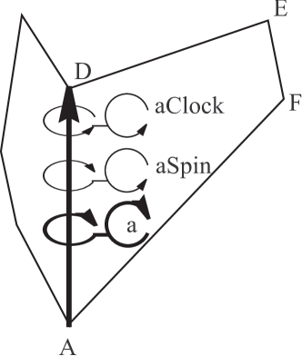
(a) (b)

Figure 2.6: The operators Clock, Spin, ENext and FNext applied to the facet edge ${<\!AD,ADFE\!\!>}$

Thus, in Figure 2.6a the facet-edge $a={<\!AD,ADEF\!\!>}$, associated with the directed edge $AD$ and with the oriented face $ADEF$, is represented by the two thick, dark gray, oriented circles. In Figure 2.6a we report also the two facet-edges that results from the application of the two operators ENext and FNext to the facet-edge $a={<\!AD,ADEF\!\!>}$. The facet-edge $a\cdot Fnext={<\!AD,BCAD\!\!>}$ is represented by the two white oriented cycles in Figure 2.6a. The facet-edge $a\cdot Enext={<\!DE,ADEF\!\!>}$ is represented by the two black oriented cycles in Figure 2.6a. In Figure 2.6b we report the facet-edges that results from the application of the two operators Clock, Spin, The facet-edge $a\cdot Spin={<\!AD,DAFE\!\!>}$ is represented by the first two oriented cycles in Figure 2.6b. The facet-edge $a\cdot Clock={<\!DA,DAFE\!\!>}$ is represented by the next two oriented cycles in Figure 2.6b.

Starting from the facet-edge ${<\!f,e\!\!>}$ and composing these four operations we can obtain:

• the previous edge in the cycle of faces that bound the oriented face $f$;

• the previous face in the oriented sequence of faces around edge $e$.

With these operations we can retrieve a cycle of edges for every face and a cycle of faces adjacent to a certain edge.

The data structure used for this representation is made up of a collection of arrays storing four pointers. For a given unoriented face and a given unoriented incident edge we recall that four possible facet-edge pairs are possible. All of them are represented by the so called facet-edge node. In the data structure presented in [57] the facet-edge node for ${<\!f,e\!\!>}$ is represented by four references. Thus the internal data structure is similar to that of the quad–edge (see Figure 2.2).

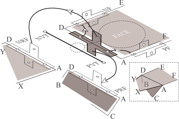
Figure 2.7: A fragment of the facet-edge data structure for three $2$-cells sharing the edge $AD$

In Figure 2.7 we report a fragment of the facet-edge data structure for three $2$-cells sharing the edge $AD$. This complex is reported in the dashed box in the lower right corner of Figure 2.7. In this figure we depict the facet-edge node (drawn in dark gray with thick border) for the for four facet-edges associated with edge $AD$ and face ADEF also denoted by $FACE$. In the same drawing we report the four facet-edge nodes referenced by this facet-edge node. These four facet-edge nodes are:

• the facet-edge node for the next and the previous facet-edge in the cycle of edges for the face $FACE$. These are denoted by $NF$ and $PF$ in Figure 2.7.

• the facet-edge node for the next and the previous facet-edge in the cycle of faces around edge $AD$. These are denoted by $NRF$ and $PRF$ in Figure 2.7.

Thus, in this data structure, face-nodes form a doubly-linked lists around each edge and a doubly linked list for each face. Note that in the original data structure presented in [57] references to the face FACE and to vertices PVT and NVT are not mentioned.

The facet-edge is represented by a record called facet-edge reference that contains a reference to a facet-edge node plus three bits to encode the possible orientation of the edge and of the facet. It can be proven [57] that is possible to implement all operations $Fnext$, $Enext$, $Spin$ and $Clock$ by transforming facet-edge references. Without entering the details of the implementation of these operators we simply note that operations $Enext$ and $Fnext$ will change the referenced face-node while operations $Spin$ and $Clock$ do not change the referenced face-node but simply alters the bits in the facet-edge reference.

The storage requirement of this data structure can be easily evaluated for a simplicial subdivision. For a simplicial subdivision we spend 12 references for each triangle in the $2$-skeleton of the modeled $3$-complex. Thus the storage requirement of this data structure is of $12f$ for a simplicial complex whose $2$-skeleton has $f$ triangles.

The original paper [57] does not present algorithms to extract topological relations nor it introduces entities to model explicitly vertices, 2-cells and 3-cells. Given a facet-edge pair ${<\!f,e\!\!>}$ it is easy to see that, in a cell subdivision, we can compute in linear time both the EF relation for an edge $e$ and the FE relation for a face $f$. Given a facet-edge incident to a given polyhedral cell it is possible to extract all facet-edges incident to that polyhedral cell. It is easy to see that for a simplicial subdivision the TE relation (recall that TE in this case stands for top-3-cell to edge) can be computed in linear time whenever a facet-edge incident to a given top 3-cell is available.

Handle Face Data Structure

The Handle-Face data structure [81] is designed to represent 3-manifolds described by cell complexes. Each cell is represented through its boundary that, in turn, is represented through the reduced FES data structure (see Section 2.2.2 and Figure 2.5a). A complete FES data structure is introduced for each $3$-cell. elements to model vertices edges and faces are duplicated for each $3$-cell.

The data structure introduce four basic topological entities (see Figure 2.8): Vertices (V), Edges (E), Faces (F) and Surfaces (S). Surfaces bounds $3$-cells.

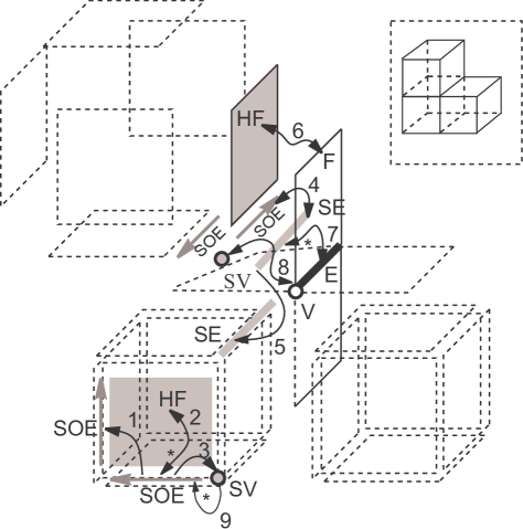
Figure 2.8: Relations among objects in the handle-face data structure for the complex made up of three cubes (fremed in the top right corner). Arrows from objects X to object Y means that every instance of object X must store a reference to the appropriate Y object.

For each vertex a distinct topological entity, called the surface vertex (SV), is introduced for each $3$-cell incident to a given vertex. For each edge a distinct topological entity, called the surface edge (SE), is introduced for each $3$-cell incident to a given edge. For each face a distinct topological entity, called the half-face (HF), is introduced for each $3$-cell incident to a given face. Note that up to two HF are introduced for each face. For each SE two oriented edges are introduced, called surface oriented edge (SOE).

The topological entities: SOE, SV, HF models each surface using the scheme of the FES. In this framework the SOE entity plays the role of the half-edge. The only difference is that the OTHERH pointer (see Figure 2.5a) is not introduced. Instead of OTHERH the surface edge (SE) node references two half-edges and is referenced by these two half-edges (we labeled this reference with $4$ in Figure 2.8). This double reference between SOE an SE plays the role of the pointer OTHERH.

Using the integer labels from Figure 2.8 we now list all references for all topological elements in the handle-face data structure. The star $*$ on one tip of a relation from X to Y denotes the ${\rm XY}^{*}$ relation (i.e. we store just one Y element in relation with X).

Following the FES scheme, in the handle-face data structure each SOE reference (1) the next SOE in the loop of edges that bounds an HF. The SOE reference also the HF (2) and the SV at its origin (3). A SV stores a reference to one (9) of the incident SOE. The SE are tied together in a cycle of references (5) of SE modeling the set of $2$-faces around an edge in a $3$-complex. The three basic topological entities: Vertices (V), Edges (E) and Faces (F) reference the corresponding lower level entities i.e., each face reference two HF and is referenced by two HF (6). Each HF stores a reference to one (relation 2 in the direction of the arrow with $*$) of the incident SOE. Each edge node is referenced (7) by each SE and points a single SOE (we recall that the star $*$ on one tip of relation 7 denotes a partial relation). Finally the vertex node V is referenced by each SV and reference (8) all the SV.

For each cell with $e$ edges this structure consumes $4e$ references to encode the SOEs and $4e$ references for the SEs (note that there are two arrows on the relations labeled with 4). To evaluate storage requirements in term of number of faces, edges and vertices we must make some assumption on the $3$-complex we are modeling. We assume that we are interested in a model with simplicial cells and we evaluate the space needed to encode a tetrahedron In this case the cell has six edges and thus the tetrahedron boundary takes 48 references. References (4) to the F node require eight more references. References (8) to the V node require other eight references. References (7) to the E node require other six references and we neglect the partial reference from E to one of its SE. References (relation 2, the arrow labeled with $*$) to a SOE incident to an HF takes other four references. References (9) to a SOE incident to an SV takes other four references. Thus in this data structure we use 78 references to model a tetrahedron. The resulting data strucutre is extremely verbose and its time efficency is not investigated in [81]. However, it is easy to see that all topological relations can be recovered in optimal time.

The paper [81] shows that the handle-face data structure supports a certain type of editing operations (the so called Morse operators) performed by attaching handle-bodies to an existing manifold.

The Three-dimensional Symmetric Structure

In [33] is studied the problem of representing simplicial decomposition for the the class of $3$-manifolds with boundary. To this aim one can model directly the four topological entities: tetrahedra (T), triangles (F), edges (E) and vertices (V) and store some of the relations between these entities. The Three-dimensional Symmetric Structure (TSS) stores relations TF, FT, FE and EV and stores, for each vertex an incident edge (i.e. the ${\rm VE}^{*}$ relation) and for each edge an incident face (i.e. the ${\rm EF}^{*}$ relation). Since each tetrahedron has four triangular faces the TF relations can be stored using $4t$ references. Since each triangular face has three edges the FE relations can be stored using $3f$ references. Since each edge has two incident vertices the EV relations can be stored using $2e$ references. The partial relations ${\rm VE}^{*}$ and ${\rm EF}^{*}$ takes respectively $v$ and $e$ references. Thus this extension of the simmetric structure to $3$-manifolds takes $8t+3f+3e+v$ references to encode a simplicial $3$-complex.

It can be proven [33] that the EF relation can be recovered in time proportional to the size of the output. This can be done by recovering first a face incident to a given edge $e$ with the ${\rm EF}^{*}$ relation. Then using the FT and the TF relations we find all tetrahedra incident to edge $e$ and with relation FE we retrieve the faces incident to $e$.

Using the algorithm for the EF extraction and the ${\rm VE}^{*}$ relation we can build the VE relation combining the EF, FE and EV relations. In both methods more elements than what is needed are visited but it can be proved that the amount of unnecessary visits has an upper bound that is linear with respect to the size of the output. Thus the EV can be extracted in linear time, as well. Combining the stored relations and the EF and VE relations it can be proved [23] that all topological relations can be extracted. It can be proved, using results in Section 9.2.2, that actually all topological relations can be computed in a time that is linear with respect to the size of the output.

Comparison for $3$-manifold modeling

The following table summarizes space requirements for the Facet Edge [57] data structure, the Handle-Face [81] data structure and for the extension of the symmetric data structure to $3$-manifolds (TSS). To compare this with the TSS we assume that we have to model a simplicial $3$-complex.

Space Requirement	Data Structure
$78t$	Handle–Face
$12f$	Facet-Edge (vertices and tetrahedra not explicitly modeled)
$t+18f$	Facet-Edge (vertices and tetrahedra explicitly modeled)
$8t+3f+3e+v$	TSS

To compare the storage requirements of the three approaches we use the relations $f\leq 4t$, $e\leq 6t$, $v\leq 4t$, $6e\leq 4f$, and $4v\leq 4f$. Note that we reach the upper bound (i.e., $f=4t$, $e=6t$, $v=4t$, $6e=4f$ and $4v=4f$) for a simplicial $3$-complex where each simplex is a distinct connected component (we called such a complex a totally exploded complex). These relations holds for all $3$-complexes that can be assembled, starting from a totally exploded tetrahedralization, gluing two triangles together. It can be proven (see Property 7.4.3 Parts 1 and 3 ) that all $3$-manifolds can be assembled in this way.

Note that $6e\leq 4f$ and $4v\leq 4f$ holds in a totally exploded tetrahedralization and there is no way to glue two triangles together without identifying at least a pair of points and two pairs of edges. Thus, every time we glue together two triangles, we decrease $f$ of one unit we decrease $v$ of at least one units and we decrease $e$ of at least two units. Thus $6e\leq 4f$ and $4v\leq 4f$ must hold in every complex assembled in this way and in particular it must hold in a $3$-manifold.

Using $f\leq 4t$, $e\leq 6t$ and $v\leq 4t$ we have $t+18f\leq 73t$ and $8t+3f+3e+v\leq 42t$. This shows that the handle-face data structure is the most expensive data structure and its storage cost is more than 1.86 times the storage cost of the TSS. Next using $6e\leq 4f$ and $4v\leq 4f$ and the fact that. in a $3$-manifold $4t\leq 2f$ we have that storage requirement for the TSS i.e. $8t+3f+3e+v$ can be written as $t+7t+3f+3e+v\leq t+3.5f+3f+2f+f=t+9.5f$. This proves that the TSS data structure is more compact than the facet–edge data structure even if we consider the original version of the facet–edge using just $12f$ pointers. The TSS saves $8.5f$ references over the facet-edge. Using $4t\leq 2f$ we have that this saving represent at least the 46% of the storage requirements of the facet-edge. Thus the facet–edge require more than 1.85 times the storage used by TSS. The above analysis is summarized in the following table that shows lower bounds for space requirements normalized vs. space requirements for the TSS.

Normalized Space Requirement	Data Structure
$\geq 1.86$	Handle–Face
$\geq 1.85$	Facet-Edge
$1$	TSS

2.2.3 Dimension independent data strucutres for encoding cell complexes

In this section we report four approaches to dimension independent modeling: the cell-tuple approach [22], the Winged Representation [103], the n-G-maps [78] and the Selective Geometric Complexes (SGC) [112]. One thing to note is that all these approaches can model $d$-manifolds but surely, for each one of these approaches, the representation domain is larger than the class of $d$-manifolds. In general we have that non recognizability of $d$-manifolds for $d\geq 6$ (see Property 3.5.3) implies that it is not possible to have a dimension independent representation whose applicative domain is exactly the class of $d$-manifolds. Any algorithm that will encode a generic $d$-complex into such a representation will act as a decision procedure for the class of manifolds. None of the above approaches, with the exception of SGCs, can model completely the non-manifold domain. The SGC can model the full generality of the non-manifold domain. We also mention that in [44], is presented an extension of n-G-Maps that also models the whole non-manifold domain.

As we anticipated, the modeling approach in this class have a stronger relations with the results of this thesis. In Chapter 9 we extend the winged representation to the non-manifold domain. Another byproduct of the results in this thesis is the exact definition of the representation domain for the winged representation that happens to be the set of quasi-manifold that, in turn, is the representation domain of n-G-maps.

Selective Geometric Complexes (SGC)

SGC [112] is a modeling scheme based on a notion of cell complex similar to CW complexes. A regular finite CW complex for a metrizable topological space $X$ (see for instance §7.3 in [63]) is a collection $\Gamma$ of subsets of $X$, called cells, such that:

• for each cell $c$ there exist an integer $k\geq 0$ such that $c$ is homeomorphic to the open $k$-ball $B^{k}=\{x\in{\rm I\kern-1.99997ptR}^{k}|\|x\|<1\}$ and the closure of $c$ is homeomorphic to a closed $k$-ball;

• $\Gamma$ is a partition of $X$;

• the boundary of each $k$-cell is homeomorphic to the $(k-1)$-sphere $S^{k-1}$ and can be expressed as the union of cells in $\Gamma$.

A $k$-cell is a cell homeomorphic to $B^{k}$.

The cell concept in CW complexes is devised to attack topological problems, whereas SGC cells have been tailored to the needs of geometric modeling. As we quote form [112], the differences lies almost exclusively in the concept of what constitutes the fundamental entity: the cell. SGCs are a compromise between simplicial complexes and CW complexes. CW complexes are, by far, too abstract. In fact, every solid, homeomorphic to a closed $3$-ball, can be expressed by the same CW complex. For representing such a solid it is sufficient a CW complex, whose combinatorial structure reduces to the triplet $\{p,S^{2}-p,B^{3}\}$ (being $p$ any point of $S^{2}$). We have that cell $c_{0}=p$ is a point, i.e., a 0-cell. The cell $c_{2}=S^{2}-p$ is homeomorphic to $B^{2}$ i.e., a 2-cell. The last cell $c_{3}=B^{3}$ is a a 3-cell. The three cells are organized so that $\partial c_{3}=c_{2}+c_{0}$; and $\partial c_{2}=c_{0}$.

On the other hand, simplicial complexes are too detailed. Indeed, infinitely many simplicial representations are possible, for a given topological space. Even if, we just consider complexes with a minimal number of simplices, we are left with a non-unique representations. For a cubic surface, for example, we have $2^{6}$ different, simplicial complexes with twelve triangles.

For this cubic surface, for example, SGC provides the quite ”natural” representation with: 6 2-cells, 12 1-cells and 8 0-cells. However, SGC are, still, fairly abstract. Indeed, with SGC, we can express, with a finite complex, some unbounded domains. SGC can also code: non-manifolds, open set, domains with missing internal points and non regular simplicial complexes. So, SGC stands midway between CW and simplicial complexes, supporting natural and unique representations. The expressive power of SGC cells is quite broad since they can encode cell complexes with open and closed cells and with cells with internal vertices and edges.

SGC cells are defined using concepts from the theory of algebraic varieties and stratification. An algebraic variety [133] is any closed subspace of the Euclidean space ${\rm I\kern-1.99997ptR}^{d}$ that is the locus of common real zeros of a finite set of real polynomials in $d$ variables. A variety that cannot be decomposed as the union some other varieties is called an irreducible algebraic variety. An irreducible algebraic variety $V$ can still be partitioned, using differential properties, into a regular part $R$ and a singular part $S$. It can be proved that the set of connected components of $R=V-S$ must be a finite set of open manifolds that are sub-manifolds of $V$ [21, 7]. Each of these sub-manifolds is called an extent of $V$.

Furthermore, it can be proven that the set of singular points $S$ is both a closed set and a variety. Thus $S$ will have its extent too. These extents will be considered as extents of $V$. too. The theory of stratification [30, 64, 126] guarantees that $V$ can be decomposed into the disjoint union of a set of connected open sub-manifolds each sub-manifold being included into an extent of $V$. This set is called a manifold decomposition of $V$. A manifold decomposition ${\mathcal{M}}$ has a cellular structure, i.e., the boundary of an element in a manifold decomposition of $V$ (denoted by ${\mathcal{M}}$) can be expressed as the disjoint union of a finite set of elements in ${\mathcal{M}}$.

With this theoretical foundation SGC defines a cell $c$ as any connected open subset of an extent of an algebraic variety. We will denote with $c.E$ the extent in which cell $c$ is contained.

A SGC ${\mathcal{C}}$ is any collection of disjoint cells $c_{i}$ such that the boundary of each cell is the disjoint union of a finite set of elements in the SGC ${\mathcal{C}}$. Furthermore, for all cells $c_{i}$ on the boundary of a cell $c$, cells $c_{i}$ in a SGC are constrained to stay either on the interior of the extent $c.E$ (i.e. $c_{i}\subset c.E$) or completely outside the extent $c.E$ (i.e., $c_{i}\cap{c.E}=\emptyset$).

This definition of SGC cells guarantees that we can always find a common refinement of two intersecting cells from two different SGC. The intersection of two algebraic varieties yields an algebraic variety of lower dimension. From these intersections we can select new boundary cells, that cut the intersecting cells of higher dimension. This cut defines the common refinement we need. Obviously, this approach assumes that we are able to computationally intersect algebraic varieties without too many problems.

Cells in SGCs are defined so that we can always find a SCG complex that describes the intersection of two cells. This choice is the key factor that allows SCG to support a rich set of operations including Boolean operations, boundary and interior operation and regularized boolean operations.

The encoding of adjacency relations in SGCs is done using as a complete incidence graph [53]. In fact each cell $c$ bears a reference to the cells that are on the boundary of $c$ and to cells that have $c$ in their boundary. This seems quite space consuming if compared with data structures we previously reviewed. However it is clearly unfair to compare the combinatorial structure of an SGC complex against, let say for instance, the combinatorial structure of a simplicial subdivision. In SGC complexes are modeled with a cell complex using quite complex cells. Thus, in SGC, the structure of the cell complex, represented via an incidence graph, can be regarded as an upper layer that ties together quite complex cells. In this we see a relationship between SGC and our two layer data structure devised in Chapter 9.

SGC cells are then grouped together using a generic cellular structure encoded using the incidence graph. As a result, with SGC, we can handle any kind of non-manifold complexes, including non-regular complexes with dangling edges and isolated points.

SGCs supports uniqueness of representation. Different SGC representations are possible for a given topological space. However SGCs representation can be ordered so that, redundant SGC representations are recognized and just one, minimal, CSG representation is maintained. It is possible to define a simplification procedure that compresses redundant SGCs to such a minimal representation. SGC simplification, actually induces a poset structure over SGC complexes. To see how this takes place we need, again, to introduce some definitions.

We will say that two cells of the same extent can be joined iff they can be merged into one deleting their common external boundary. We will say that a SGC $C$ can be simplified iff there are two or more cells in $C$ that can be joined. If a new complex $C^{\prime}$ results from a set of simplifications performed on $C$, then, we will say that $C$ will be a refinement of $C^{\prime}$ and we will write $C^{\prime}<C$. For instance in Figure 2.9 we have that the complex in (a) is a refinement of the complex in (b).

Figure 2.9: Operations in SGC: A non minimal SGC (a), then its minimal SGC (b), then its regularized version (d) obtained taking the closure of the interior of (b). Topological operations in SGC: SGC (c) is the interior of (b); (d) is the closure of (c); (f) is the boundary of (d); (e) is is the result of a boundary operation on the non minimal SGC in (a).

The notion of refinement defines a partial order over the class of SGC. In the poset ordered by the refinement relation $<$ for every SGC $C$, there is a lower minimal element $\widehat{C}$, such that $\widehat{C}<C$. Such a minimal element $\widehat{C}$ can, actually, be computed with a simplification algorithm. If $A$ and $B$ represent tha same topological space, then, it can be proved that, $\widehat{A}=\widehat{B}$. Hence, we can say that SGC provides a unique representation for a given topological space that can be subdivided as a SGC. For instance in Figure 2.9 we have that the SGC in (b) is the minimal representation for the complex in (a). From a minimal SGC representation of a topological space $CC$, we can extract a SGC representation for the interior $\stackrel{{\scriptstyle\circ}}{{CC}}$ and the boundary $\partial CC$ of $CC$. A SGC complex for the interior $\stackrel{{\scriptstyle\circ}}{{CC}}$ of $CC$ is obtained, selecting all the cells of maximal dimension in the SGC for $CC$ (in Figure 2.9 in (c) we have the interior of the SGC in (a)).

The boundary of the interior $\stackrel{{\scriptstyle\circ}}{{CC}}$ can be obtained selecting the cells of $CC$, that are on the boundary of cells in $\stackrel{{\scriptstyle\circ}}{{CC}}$ (in Figure 2.9 in (f) we have the boundary of the SGC in (c)). We note that, obviously, we obtain wrong results if we apply those definitions to a non-minimal SGC. For example, Figure 2.9 (e), is what remains if we take the boundary of the interior of the SGC in (a). Recall that the SGC in (a) is a non minimal, version of the SGC in (b). The complex in (e) is usually called the 1-skeleton of (a).

We have seen that we can, easily, compute $\partial\stackrel{{\scriptstyle\circ}}{{CC}}$. However, in general, we are not able to compute $\partial CC$. However, if $CC$ is regular, then $CC=\overline{\stackrel{{\scriptstyle\circ}}{{CC}}}$ and then $\partial CC=\partial\stackrel{{\scriptstyle\circ}}{{CC}}$ ($\overline{A}$ is the topological closure of $A$). If $CC$ is not regular, but it is closed, then we can extract a regularized version of $CC$, taking $\overline{\stackrel{{\scriptstyle\circ}}{{CC}}}=\stackrel{{\scriptstyle\circ}}{{CC}}\cup\partial\stackrel{{\scriptstyle\circ}}{{CC}}$ (the SGC in Figure 2.9 (d) is the regularized version of the complex in (a)).

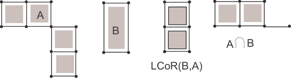
Figure 2.10: On the left two SGC $A$ and $B$. In the middle the LCoR(B,A). On the right, non-minimal SGC for $A\cap B$.

A nice feature of SGC is that the refinement partial order $<$ always admits a least compatible refinement ($LCoR$) for any pair of elements. We say that $A$ and $B$ are compatible, if their common part, $A\cap B$ is represented by the same complex both in $A$ and in $B$. For instance, in Figure 2.10 we have that $A$ and $B$ are not compatible. If we take two SGCs $A$ and $B$ there always exists a pair of minimal compatible SGCs $A^{\prime}$ and $B^{\prime}$ such that $A<A^{\prime}$ and $B<B^{\prime}$. The pair of complexes $\{A^{\prime},B^{\prime}\}$ will be denoted by $Subdivide(A,B)$.

In [112] is presented an algorithm that compute $Subdivide(A,B)$. This is based on the joint computation of the least refinement of $A$ that can be made compatible with respect to $B$ (we will denote this complex with $LCoR(A,B)$) and of the least refinement of $B$ that can be made compatible with respect to $A$ (i.e. $LCoR(B,A)$)

We note that, in general, $LCoR(A,B)\neq LCoR(B,A)$. Referring to Figure 2.10 we have that: $LCoR(A,B)=A$ and $LCoR(B,A)$ is the SGC in the middle of Figure 2.10. Furthermore, $LCoR(A,B)$ is not compatible with respect to $B$, but it is compatible with $LCoR(B,A)$. With this notation, we can, finally, describe $Subdivide(A,B)$ as $Subdivide(A,B)={<\!LCoR(A,I),LCoR(B,I)\!\!>}$ where $I=LCoR(A,B)\cap LCoR(B,A)$ is the intersection. Then referring to Figure 2.10 we have that $Subdivide(A,B)={<\!A,LCoR(B,A)\!\!>}$.

When the SGCs for $Subdivide(A,B)$ is available, then we can extract, from $Subdivide(A,B)$, a SGC for both $A\cup B$ and $A\cap B$. For example, in Figure 2.10 we compute $A\cap B$ taking cells, that are both in $LCoR(A,B)$ (i.e. A) and $LCoR(B,A)$ and obtain the complex on the right of Figure 2.10. Then, referring back to Figure 2.9 (a) we simplify the SGC (a) for $A\cap B$ and obtain 2.9 (b), that is a minimal SGC. Steps in Figures 2.9 (c) and 2.9 (d) leads to the regularized version of $A\cap B$. In this way, SGC supports both Boolean operations and regularized Boolean operations.

We note that, to compute $Subdivide(A,B)$, we need to check every pair of cells in $A$ and $B$ for intersection. This might require $\Theta({\|{A}\|}{\|{B}\|})$ intersections between pairs of algebraic varieties. In [112] a complexity analysis for this operation is not reported.

In conclusion, SGC supports both Boolean and regularized Boolean operations. It is possible to define a simplification procedure that compresses redundant SGCs to its minimal representation SGC with respect to  the ordering induced by the simplification notion. A SGC usually has an extremely compact, combinatorial structure, while more complex geometric information might be used to code cells. Therefore, the adoption of SGC representations shifts the complexity towards the geometry of cells.

The Cell-Tuple

The cell-tuple offer a scheme to encode any CW complex of a d-manifold. Given a finite regular CW complex $\Gamma$ for a $d$-manifold ${\mathcal{M}}$ we define a subdivided manifold, as the pair $\{{\mathcal{M}},\Gamma\}$. A cell-tuple for the subdivided manifold $\{{\mathcal{M}},\Gamma\}$ is any sequence of $d+1$ cells of $\Gamma$, $t=(c_{0},\ldots,c_{d})$ such that $c_{i}$ is a cell of dimension $i$ and such that $c_{i}$ is a face of $c_{i+1}$.

The cell tuple structure for a subdivided $d$-manifold $\{{\mathcal{M}},\Gamma\}$ is given by the set ${\mathcal{T}}$ of all cell-tuples for $\Gamma$ together with a set of symmetric relations, denoted by ${\rm switch}_{i}$, such that, two cell-tuples $\tau$ and $\tau^{\prime}$ are in relation with respect to ${\rm switch}_{i}$ if and only if  they differ just for the $i$-th cell. It is easy to see that for a top $d$-cell that is a $d$-simplex we must introduce ${(d+1)!}$ cell-tuples in ${\mathcal{T}}$.

Figure 2.11: The graph of cell-tuples (with dashed arcs) for the complex made up of the the two square faces $A=uvwz$ and $B=wxyz$ and of the surrounding unbound face $C$. Small dots labeled with triples are cell-tuples. Dashed arcs links two cell tuples that are in the ${\rm switch}_{i}$ relation being $i$ the arc label.

The cell-tuple structure can be represented by a graph whose nodes are the cell-tuples in ${\mathcal{T}}$ and such that there is an arc (labeled with $i$) in between the two cell-tuples $\tau$ and $\tau^{\prime}$ whenever $\tau$ and $\tau^{\prime}$ are in relation with respect to  ${\rm switch}_{i}$. An example of this graph representation is in Figure 2.11.

It can be proven that the relations ${\rm switch}_{i}$ are actually functions, i.e. there is just one edge labeled with $i$ leaving from any node in the cell-tuple graph. Thus, all the nodes in this graph must be of order $(d+1)$. It can be proven [22] that there is a bijection between $i$-cells in the complex $\Gamma$ and cycles that do not contain arcs labeled with $i$. An $i$-cell is incident to a $k$-cell if and only if  the associated cycles share some vertices. Thus all topological relations can be extracted in optimal time traversing the graph of cell-tuples.

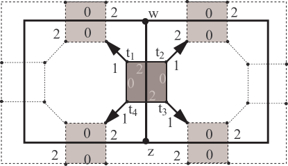
Figure 2.12: Translation of the cell tuple of Figure 2.11 into winged-edge and quad-edge

A cell-tuple structure for a subdivided $2$-manifold ${\mathcal{M}}$ can be translated into a winged-edge data structure, a quad-edge data structure, a FES and a VES. Examples of this translation for the complex of Figure 2.11 are given in Figure 2.12. A cell-tuple structure for a subdivided $3$-manifold can be translated into a facet-edge data structure. All these translations are better understood if we refer to the graph representation of a cell tuple data structure. In this graph we will call a $\{x,y\}$-orbit (or $xy$-orbit for short) a cycle whose edges are labeled only with $x$ and $y$. In a similar way we define $x$-orbits and $xyz$-orbits. With some abuse of notation, given an orbit $o$ we will call the $o$ orbit also the corresponding orbit in the algebraic cell tuple structure i.e. the set of cell tuples associated to graph vertices in the orbit. With this notation we can define how to translate a cell-tuple graph into various data structures.

To obtain a winged-edge data structure or a quad-edge data structure we consider 02-orbits. Let $o$ be the (set of cell-tuples in a) 02-orbit (in dark gray in Figure 2.12) given by $o=\{t_{1},t_{2},t_{3},t_{4}\}$ being, for instance, ${\rm switch}_{0}(t_{1})=t_{4}$, ${\rm switch}_{2}(t_{4})=t_{3}$, ${\rm switch}_{0}(t_{3})=t_{2}$ and ${\rm switch}_{2}(t_{2})=t_{1}$. For each 02-orbit $o$ we introduce a winged-edge (or a quad-edge) whose four wings (solid arrows in Figure 2.12) points the other four winged-edges (in light gray in Figure 2.12) introduced for the four 02-orbits containing, respectively, ${\rm switch}_{1}(t_{1})$, ${\rm switch}_{1}(t_{2})$, ${\rm switch}_{1}(t_{3})$ and ${\rm switch}_{1}(t_{4})$.

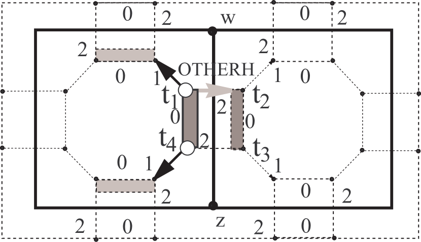
(a)

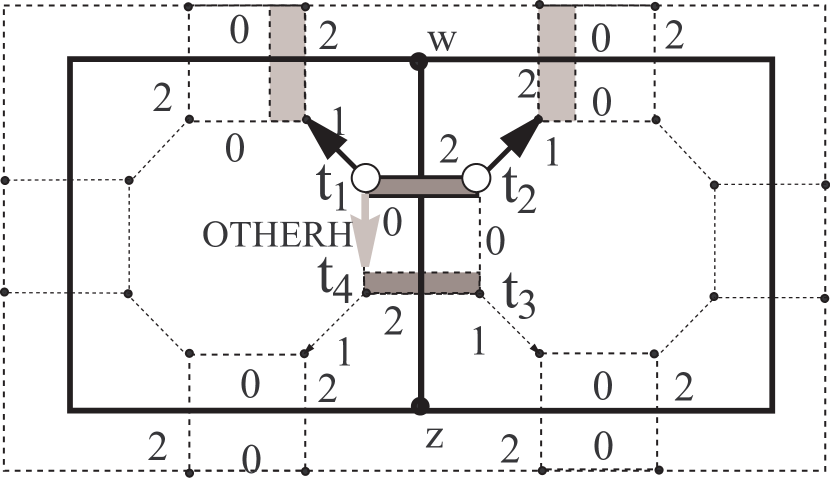
(b)

Figure 2.13: Translation of the cell tuple of Figure 2.11 into FES (a) and VES (b) data structures

To obtain a FES half edge, (see Section 2.2.1) we consider 0-orbits Let $o$ be the 0-orbit (in dark gray in Figure 2.13 (a)) given by the pair $t_{1}$ and $t_{4}$ with ${\rm switch}_{0}(t_{1})=t_{4}$. For each 0-orbit $o$ we introduce a FE half-edge whose pointer OTHERH points the half-edge introduced for the 0-orbits containing the tuple pointed by ${\rm switch}_{2}$ (in dark gray in Figure 2.13 (a)). In this case points $t_{2}$ since ${\rm switch}_{2}(t_{1})=t_{2}$. In Figure 2.13(a) the two wings points with solid black arrows the half-edges introduced for the results of the mappings ${\rm switch}_{1}(t_{1})$ and ${\rm switch}_{1}(t_{4})$.

Similarly, to obtain a VES half edge (see Section 2.2.1), we consider 2-orbits Let $o$ be the 2-orbit (in dark gray in Figure 2.13b) given by $o=\{t_{1},t_{2}\}$ . This is a 2-orbit since ${\rm switch}_{2}(t_{1})=t_{2}$. For each 2-orbit $o$ we introduce a VE half-edge whose pointer OTHERH points to the half-edge introduced for the 2-orbit containing $t_{3}$ and $t_{4}$ (in dark gray in Figure 2.13(b)). Therefore OTHERH is translated using ${\rm switch}_{0}$ indeed ${\rm switch}_{0}(t_{1})=t_{4}$. The two wings (solid black arrows in Figure 2.13 (b)) points the half-edges introduced for the orbits we can reach thru the maps ${\rm switch}_{1}(t_{1})$ and ${\rm switch}_{1}(t_{2})$.

More complex is the relation between the facet-edge (see Section 2.2.2) data structure and the cell-tuple. To understand this relation we must consider the fragment of the facet-edge structure reported in Figure 2.7. In Figure 2.14 (a) we draw the cell-tuple graph for the fragment of complex of Figure 2.7.

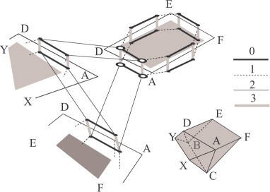
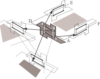
(a) (b)

Figure 2.14: Translation of the cell-tuple data structure for the complex in the lower right corner of (a) into the corresponding facet-edge data structure in (b) and also in Figure 2.7

In the graph fragment of Figure 2.14(a) we report the cell-tuples containing the face DAFE (the rectangle on the right) and the cell-tuples containing the edge DA. Note that each face is encoded as if it was surrounded by a outer space. Thus for each edge we take four cell tuples. Note that in this graph of cell tuples edges are drawn with different styles instead of using labels. A translation for these styles is reported on the left of Figure 2.14(a). We can translate this graph into the facet-edge data structure associating a facet-edge to each cell-tuple. The four large white spots in Figure 2.14(a) are translated into the four facet-edges that can be associated to the four variants of the facet edge pair ${<\!AD,DAFE\!\!>}$. However, in the facet-edge data structure facet-edge are not represented directly. In fact, the basic entity in the facet-edge data structure is the facet-edge node. Therefore, to translate the cell-tuple data structure for a subdivided $3$-manifold into a facet-edge data structure we must introduce a facet-edge node for each 03-orbit in the cell-tuple graph. This is what is represented in Figure 2.14 (b). A facet-edge node is associated with the 03-orbit (in dark gray in Figure 2.14(b)) given by $o=\{t_{1},t_{2},t_{3},t_{4}\}$ (in Figure 2.14(b) the cell-tuple $t_{i}$, for $i$ equal to 1,2,3 and 4, is the white blob labeled with $i$). We have, for $i=2,4$, ${\rm switch}_{3}(t_{i-1})=t_{i}$ and ${\rm switch}_{0}(t_{i})=t_{(i+1)mod4}$. For each 03-orbit we introduce a facet-edge node whose four references (solid arrows in Figure 2.14 (b)) points the other four facet-edge nodes introduced for the four 03-orbits containing, respectively, ${\rm switch}_{1}(t_{1})$, ${\rm switch}_{2}(t_{2})$, ${\rm switch}_{1}(t_{3})$ and ${\rm switch}_{2}(t_{4})$. The final facet-edge data structure is the one shown in Figure 2.7. This completes the description of the translation of the Cell Tuple into the Facet Edge.

The domain of representation of cell-tuples is restricted to subdivided $d$-manifolds but it can be proven [78] that the representation domain of cell-tuple is wider than this. We discuss this issue in the next section showing the relation between cell-tuples and n-G-maps.

The cell-tuple representation is extremely verbose. If we encode a simplicial subdivision of a $d$-manifold we must store, for each $d$-simplex, ${(d+1)!}$ tuples each containing $(d+1)$ elements. If we represent the cell tuple data structure through its graph we have to accomodate ${(d+1)!}$ nodes for each $d$-simplex. Each graph node is of order $(d+1)$. We can implement nodes as an array of $(d+1)$ references to other $(d+1)$ nodes. In both cases we have to use $(d+1){(d+1)!}$ reference for each $d$-simplex.

n-G-maps

The n-G-maps [78] is an implicit cell model, like the cell-tuple, but n-G-maps have an expressive power higher with respect to  cell-tuples since they can describe a subclass of pseudomanifolds, called cellular quasi-manifolds. An n-G-map model is described by a set of paste relationship $\alpha_{i}$ between primitive elements, called darts. For a $d$-dimensional space $d+1$ paste relationships are necessary. Relationships must satisfy certain constraint that enforce coherence in the representation. The three constraints are:

• each $\alpha_{i}$ must be an involution, i.e., $\alpha_{i}^{2}=\alpha_{i}$;

• $\alpha_{i}$, for $0\leq i<n$, must not have fixed points;

• $\alpha_{i}\alpha_{i+2+k}$ must be an involution for all $0\leq i<i+2+k\leq n$

Whenever $\alpha_{n}$ is also an involution the n-G-map is called closed.

When these constraints are satisfied, we can look at kernel relationships as relations that paste together darts. Pasting together darts leads to the modeled object.

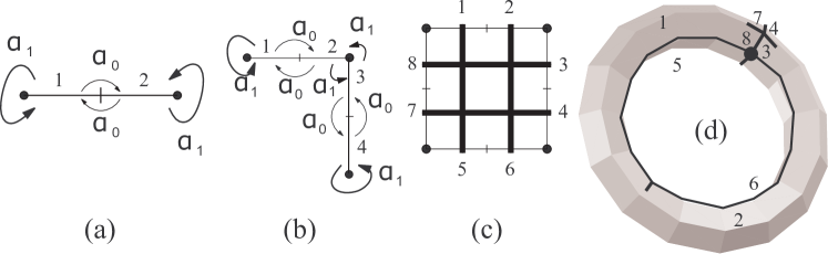
Figure 2.15: Examples of n-G-maps

In Figure 2.15 we find examples of complexes modeled with n-G-maps. From left to right we have an example of a 1-G-map formed by two darts labeled $1$ and $2$. In the complex of Figure 2.15a involution $\alpha_{0}$ is defined completely by the equation $\alpha_{0}(1)=2$ while involution $\alpha_{1}$ is the identity. Therefore the n-G-map of Figure 2.15a is an example of a non-closed n-G-map. The complex in Figure 2.15b is an example of a non-closed 1-G-map defined by $\alpha_{0}(1)=2$, $\alpha_{0}(3)=4$, $\alpha_{1}(1)=1$, $\alpha_{1}(3)=2$ and $\alpha_{1}(4)=4$. The complex in Figure 2.15c, if we do not consider the four thick black stripes, is the 1-G-map for the perimeter of a square. This is obtained using four darts and the involutions: $\alpha_{0}(1)=2$, $\alpha_{0}(3)=4$, $\alpha_{0}(5)=6$, $\alpha_{0}(7)=8$, $\alpha_{1}(1)=8$, $\alpha_{1}(2)=3$, $\alpha_{1}(4)=6$ and $\alpha_{1}(5)=7$. Note that arrow labels are omitted in Figure 2.15c. This defines a closed 1-G-map. We can transform this into the toroidal surface of Figure 2.15c by stitching together darts: 1 and 5, 2 and 6, 3 and 8, 4 and 7. In general a surface is modeled by a 2-G-map that can be obtained from a 1-G-map by introducing the involution $\alpha_{2}$ In this case the involution we need to build the toroidal surface is defined by: $\alpha_{2}(1)=5$, $\alpha_{2}(2)=6$, $\alpha_{2}(3)=8$ and $\alpha_{2}(4)=7$. This is denoted in Figure 2.15c (following the graphical conventions in [78]) by the four thick black stripes.

After these examples we can say that, in general, in n-G-maps the modeled object is built pasting together darts with $\alpha_{i}$ pasting relations. Relation $\alpha_{0}$ connects darts to form edges. For this reason the dart is usually graphically represented as a VE half-edge. Then, by connecting darts (with $\alpha_{1}$) we connect adjacent edges to form both cycles and open paths. Cycles will be used to model 2-cells. Then we connect darts in adjacent 2-cells (with $\alpha_{2}$) to form a surface with or without boundaries. Surfaces without boundary will model a 3-cells. Going on, (with $\alpha_{3}$) we can connect 3-cells and build a $3$-complex.

The representation domain of n-G-maps is the set of Cellular Quasi-manifold [80]. This class of complexes is especially relevant in this thesis and therefore we will give a deeper insight into this definition. Cellular quasi-manifold are pseudomanifolds whose cellular decomposition can be triangulated into a simplicial set that is a simplicial quasi-manifold. To introduce simplicial quasi-manifold we first need to introduce numbered simplicial sets.

A numbered simplicial $d$-dimensional set is a simplicial $d$-complex whose vertices are labeled with integers from $0$ to $d$. In each $h$-simplex of a numbered simplicial $d$-dimensional set the $h+1$ labels for vertices must be distinct. Not all simplicial complexes can become a numbered simplicial complexes adding a labeling to vertices. For instance, the boundary of the tetrahedron is an example of a $2$-complex that cannot be labeled as a numbered simplicial complex. Once that we have assigned labels 0,1,2 to three vertices of the tetrahedron, there is no vay to assign a label from 0 to 2 to the fourth vertex of the tetrahedron. Whatever will be our labeling choice we will not have distinct labels for all triangles on the boundary of the tetrahedron. This proves that the boundary of a tetrahedron is not a numbered simplicial complex. However it can be proven that is always possible to find a such a labeling for the barycentric subdivision of a given simplicial complex so that the subdivision becomes a numbered simplicial complex.

A simplicial quasi-manifold $d$-complex is a numbered simplicial $d$-complex that can be obtained from a collection of disjoint $d$-simplices identifying $(d-1)$ faces in such a way that at most two $d$-simplices share a $(d-1)$-face. Cellular quasi-manifold are defined as pseudomanifolds that have a triangulation that is a simplicial quasi-manifold.

Note that according to the original definition the boundary of the tetrahedron is a simplicial complex that is a cellular quasi-manifold but it is not a numbered simplicial quasi-manifold.

In this thesis we will consider only simplicial subdivision, therefore we will use the term quasi-manifold to denote a simplicial complex that is a cellular quasi-manifold. It is easy to show that all and alone the cellular quasi-manifold that are simplicial can be obtained from a collection of disjoint $d$-simplices identifying $(d-1)$ faces in a way that at most two $d$-simplices share a $(d-1)$-face.

For surfaces (i.e. 2-manifolds) it has been proven [54] that all subdivision of $2$-manifolds can be expressed by gathering cells homeomorphic to a disk and by identifying edges. Thus we can say that 2-G-maps can express all and alone surfaces and quasi-manifold $2$-complexes coincide with $2$-manifolds. In higher dimension we can always find a bijection between classes of topological spaces and sub-classes of n-G-maps. However, in general, it is unknown which is class of topological spaces that can be expressed by gathering $d$-cells homeomorphic to a $d$-ball and by identifying cell $(d-1)$-faces.

Even if the n-G-maps modeling cannot express the whole non-manifold domain, n-G-maps are the most expressive scheme among implicit cell representations. Their expressive power is beyond that of cell-tuples. A representation based on chains of n-G-Maps [44] can be used to represent arbitrary cell complexes with a mix of open and closed cells. In this scheme, we have a 2-level hierarchy where both chains and cells must be represented. A straightforward implementation of n-G-Map chains must implement explicitly both chains and n-G-maps, the latter being used to represent cells.

There is a tight relation between cell-tuples and n-G-maps as abstract combinatorial objects. According to [22] one can translate a cell-tuple into an n-G-map by introducing a dart $d(t_{i})$ for each cell tuple $t_{i}$ and by defining the involution $\alpha_{k}$ as $\alpha_{k}(d(t_{i}))=d({\rm switch}_{k}(t_{i}))$. A minor difference between n-G-maps and cell-tuples is in the way they handle boundaries. The cell-tuple approach assumes that the modeled $d$-complex in surrounded by a special $d$-cell $c_{\infty}$. On the other hand n-G-maps bend darts into fixpoints for the involution $\alpha_{n}$ to express boundaries. To cope with this distinction one have to pre-process a cell-tuple representation before translating it into n-G-maps and redefine ${\rm switch}_{n}(t)$ as ${\rm switch}_{n}(t)=t$ whenever the cell-tuple ${\rm switch}_{n}(t)$ contains $c_{\infty}$.

On the other hand, following [77], one can find examples of 2-G-maps for a certain subdivision of a subdivided $2$-manifold that cannot be translated directly into a cell-tuple. Let consider for instance the triangle $A=xyz$ in Figure 2.16 (a) with an internal point $t$ and an internal edge $d$. This correspond to the 2-G-map in Figure 2.16 (b) where darts 1 and 4 and darts 2 and 3 are tied together by the involution $\alpha_{2}$ (thick black stripes). This cannot be expressed as a cell-tuple structure introducing a cell-tuple for each dart. If we attempt to do this we end up in a cell-tuple structure containing the three tuples $(A,b,x)$,$(A,c,x)$ and $(A,d,x)$. This is not allowed in the cell-tuple scheme. Indeed, in this case, we have that relation ${\rm switch}_{1}$ is not a function. In fact, there are two possible results when ${\rm switch}_{1}$ is applied to each of these three tuples above.

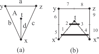
Figure 2.16: An example of a 2-G-maps that cannot be translated directly into a cell-tuple

An implementation of n-G-maps is proposed [16, 76] using $d+1$ pointers for each dart in a $d$-dimensional complex. In a simplicial subdivision each $d$-simplex will require ${(d+1)!}$ darts and thus $(d+1){(d+1)!}$ references.

The Winged Representation

The winged representation [103] is a dimension independent modeling approach for simplicial subdivisions. The domain of the winged representation is the subclass of the topological sub-spaces of ${\rm I\kern-1.99997ptR}^{n}$ that can be represented by a uniformly dimensional simplicial subdivision such that a $(d-1)$-simplex is adjacent at most to two $d$-simplices. The original Winged Representation, for a uniformly dimensional $d$-complex $\Omega$, is a pair $(\Omega^{[d]},{\mathcal{A}})$ where $\Omega^{[d]}$ is the subset of the $d$-complex $\Omega$ made up of all $d$-simplices in $\Omega$ and ${\mathcal{A}}$ is an adjacency function that associates each $d$-simplex with the $(d+1)$-tuple of $d$-simplices that are adjacent to it. Both vertices and $d$-simplices are represented through indexes and $d$-simplices in $\Omega^{[d]}$ are represented as (d+1)-tuples of vertex indexes. Thus the data structure for $\Omega^{[d]}$ will be a function that gives, for each top simplex index $t$, the $(d+1)$ indexes of the vertices in $t$. This is often called the TV relation (Top simplex to Vertex). Similarly the data structure for the adjacency function ${\mathcal{A}}$ will be a function that gives, for each top simplex index $t$, the $(d+1)$ indexes of the top simplices adjacent to $t$. For simplices that are not adjacent exactly to $(d+1)$ $d$-simplices, the special symbol $\bot$ is used, at some places, in the corresponding $(d+1)$ tuple to mean ”no adjacency”. This is often called the TT relation (Top simplex to Top simplex). For this reason the winged representation is sometimes called the TV,TT data structure or indexed data structure with adjacency.

The original work introducing the name ”winged representation” [103] defines a functional language that allows to manipulate polyhedra that are geometric realizations of winged representations. A rich set of operations is provided including: boundary operator, extrusion operators, editing through the application of simplicial maps and set theoretic operations. In particular the algorithm for boundary extraction [47] shows that one can effectively navigate the simplicial complex using relations ${\mathcal{A}}$. In spite of this flexibility the winged representation is extremely compact since it uses $6f$ references to encode a manifold surface and $8t$ references to encode a tetrahedralization. In general, $2(d+1)$ references are needed for each top $d$-simplex in the modeled $d$-complex. In Appendix B, we give an optimization procedure that can encode implicitly some information in this representation saving $v$ references.

The problem of extracting all topological relations out of this representation for $d$-manifolds is briefly reported in the following. A first problem is to extract, for a given $0\leq m\leq d$, all $m$-simplices incident to a given vertex $v$. The extraction of these, vertex based, topological relations can be performed adding $v$ references to encode the partial relation ${\rm VT}^{*}$ that gives, for each vertex, an incident $d$-simplex. The optimization in Appendix B, encodes implicitly, this relation, as well.

In order to extract, for given $0<i<m\leq d$, all $m$-simplices incident to a given $i$-simplex $\gamma$, can introduce similar partial relations (denoted by $V^{i}T$) that gives, for each $i$-simplex, for $0<i<d$, an incident $d$-simplex.

In this thesis (see Section 9.5.5) we designed a trie [39] based data structure that can encode all these $V^{m}T$ partial relations using less than three references for each $m$-simplex for $0\leq m\leq(d-1)$ and less than two references for each $(d-1)$-simplex. (See Property 9.5.11).

Thus, we can encode the winged representation and all these partial relations $V^{i}T$ for our simplicial complex using $6f+2e+3v$ references for surfaces and $8t+2f+3e+3v$ references for tetrahedralizations. Using the optimization in Appendix B this reduces to, respectively, $6f+2e+v$ references for surfaces and $8t+2f+3e+v$ references for tetrahedralizations.

For a simplicial subdivision of a $2$-manifold we have $3f\leq 2e$ and thus we have an storage requirement smaller than $6e+v$. For a closed manifold homeomorphic to a sphere we have $v=(6+e)/3$ and thus the storage requirement for this kind of surface an optimized winged representation takes less than $6.3e+2$, thus being more compact than all other solutions so far presented. We recall that the best storage requirement for $2$-manifolds, up to now, was $8e$ provided by the symmetric data structure (see Table 2.2).

For a $3$-manifolds the winged representation is more compact than the symmetric structure for $3$-manifolds (recall that in Section 2.2.2 we have shown that the symmetric structure takes $8t+3f+3e+v$). Thus, also for three manifolds, an optimized winged structure is the most compact solution for a tetrahedralization.

It can be proven (see Properties 9.4.4, 9.4.6, 9.4.7, 9.5.5 and 9.5.8) that, for a $d$-manifold, for $d=2$ and $d=3$, all topological relations can be extracted in linear time from the winged representation.

In this thesis we will study the winged representation in order to extend it to an efficient data structure to encode the components of our decomposition. Thus several results in this thesis are linked with this data structure. A brief discussion of these links is reported at the end of this chapter.

2.2.4 Non-Manifold Modeling Data Structures

In this section we review some modeling approaches that have been devised to model cellular subdivisions of solid objects with non-manifold situations. We first note that all these approaches assume that at most two $3$-cells in a $3$-complex shares the same $2$-face. Thus, the intended modeling domain coincides with the subset of $3$-polyhedra embeddable in ${\rm I\kern-1.99997ptR}^{3}$. In related literature we encounter different subclasses of this modeling domain. The term r-set [109] is used to denote the set of solids that can be expressed as cellular complexes where all cells have dimension $3$. An r-set has the property that it coincides with the closure of its interior.

A proper subclass of r-sets is the class of manifold solids that is simply the class of solids bounded by a geometric realizations, in ${\rm I\kern-1.99997ptR}^{3}$, of a closed orientable $2$-manifold surface. Manifold solids can be built with a finite number of finitary operations called Euler operators [109, 62]

The class of r-sets that are not collections of manifold solids is called the set of non-manifold solids. Within this class five types of non-manifold situations can occur (sometimes called special notches) The are shown in Figure 2.17 from (a) to (e).

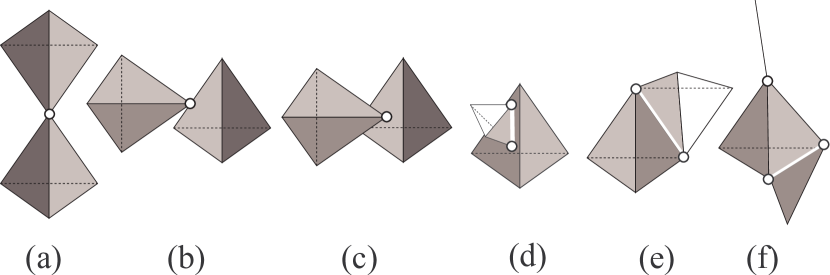
Figure 2.17: Examples of r-sets that are non-manifold solids with five different types of special notches (from a to e) and of pseudomanifold solids (from a to c). In (f) we have a non-manifold solid with dangling edges and dangling faces. In white, in each solid, we have the set of points that are not manifold points according to the topological definition of manifoldness.

The subclass of non-manifold solids where conditions of Figures 2.17 (d) and 2.17 (e) do not occur is called the class of pseudomanifold solids. Note that special notches are non-manifold situations also in the boundary of the solids. Furthermore the boundary of a pseudomanifold solid is a pseudomanifold surface.

Finally we have that the class of $3$-polyhedra imbeddable in ${\rm I\kern-1.99997ptR}^{3}$ is more general than the class of r-sets since these solids might have dangling edges and dangling faces. In Figure 2.17(f) we have a complex with a dangling edge and a dangling triangle. All the data structures listed in this section can model this, more general, class of solids. We will refer this super-class of non-manifolds as a realizable non-manifold (in ${\rm I\kern-1.99997ptR}^{3}$) while the term non-manifold will be reserved to the topological concept. In this thesis we treat this larger class of ”non-manifolds” and we do not assume embedding in ${\rm I\kern-1.99997ptR}^{3}$ unless explicitly stated.

We note that data structures listed in this section cannot model all non-manifold $3$-complexes. For instance the complex (embeddable in ${\rm I\kern-1.99997ptR}^{4}$), consisting of three tetrahedra sharing a triangle, cannot be modeled with approaches listed in this section.

A second point to note is that many of the reviewed approaches present both a concrete data structure and a set of operators to stepwise build the associated concrete data structure. For instance Weiler’s work [127] defines a set of operators called NMT that support the construction of a realizable non-manifold. Other approaches defines a set of operators that can modify a non-manifold solid preserving some sort of invariant. This invariant is usually presented as an extension of the Euler-Poincare formula for the non-manifold domain. The related operators are therefore called generalized Euler operators. In [89, 137, 73], for instance, different extension of the Euler-Poincare formula are presented and related sets of Euler operators are introduced. This approach, follows the work of Mantyla [85] that shows that the Euler operators are both complete and sound for the class of two-manifolds. In particular the strong result in Weiler’s work is the fact that he gave an inversion algorithm for the Euler operators [127] producing a sequence of Euler operations to build a given two-manifold.

The problem of creating a non-manifold data structure, when no sequence of operations is available, is partially addressed in [90]. In this paper is devised an out-of-core implementation of an algorithm that takes a (possibly huge) unstructured list of triangles in a STL input and builds a, possibly un-coherent, non-manifold data structure called LEDS. However, if a daemon properly present triangles in the STL file, in a certain order, then the algorithm can output a LEDS that is topologically coherent with the non-manifold solid it describes. In a companion paper [91] this requirement is mitigated with a slicing algorithm. This algorithm requires to have all triangle normals pointing out of the solid they bound. With this information a coherent topology is obtained.

In this thesis we describe the abstract notion of the decomposition of a simplicial $d$-complex and design algorithms to build and navigate a compact data structure that can represent generic, non-manifold, simplicial $d$-complexes using the result of the decomposition process. In this framework the definition of construction operators for this data structure is bypassed. Therefore the related literature on non-manifold operators, is neglected in this chapter. In this we follow the approach in [90] and we operate on an unordered set of simplices. However we do not assume a particular ordering for our input and yet we produce a coherent data structure from which we can extract all topological relations.

A short discussion on the possible relation between the decomposition problem and non-manifold Euler operators is discussed at the end of this chapter.

The three data structures we are going to review in this section about non-manifold data structures are: the Radial–Edge data structure (RES) [130], the Tri-Ciclic Cusp (TCC) [59] and the Partial Entity data structure (PES) [73] The RES data structure is historically the first proposal for cellular subdivisions of realizable non-manifolds. The similar data structures [59, 137, 73, 92] are basically more compact revision of the radial–edge data structure. Related paper points out some pitfalls of the RES and propose some variation to correct it.

Radial Edge

The Radial Edge Structure (RES) [130] is a modeling approach where a realizable non-manifold is represented by a set of basic elements called uses. Each use encodes a specific pair of instances of topological elements (i.e. vertices, faces, edges, etc. ) in some adjaceny relation. For instance, the edge use is the encoding of an edge-face pair within the ternary relation among edges. faces and cells.

There are seven topological elements that are considered in the RES. These are: the region, the shell, the face, the loop, the edge and the vertex: We report here the origial description of these seven RES topological entities. Between parenthesis we report the shorthands used in Figure 2.18 to denote the RES topological entities.

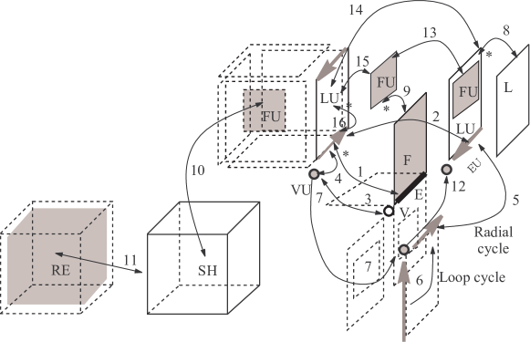
Figure 2.18: Topological entities and uses in a radial–edge data structure together with the mutual references as in BRL-CAD [10] implementation

A model is a single three-dimensional topological modeling space, consisting of one or more distinct regions of space. A model is not strictly a topological element as such, but acts as a repository for all topological elements contained in a geometric model

A region (RE) is a volume of space. There is always at least one in a model. Only one region in a model may have infinite extent; all others have a finite extent, and when more than one region exists in a model, all regions have a boundary.

A shell (SH) is an oriented boundary surface of a region. A single region may have more than one shell, as in the case of a solid object with a void contained within it. A shell may consist of a connected set of faces which form a closed volume or may be an open set of adjacent faces, a wireframe, or a combination of these, or even a single point.

A face (F) is a bounded portion of a shell. It is orientable, though not oriented, as two region boundaries (shells) may use different sides of the same face. Thus only the use of a face by a shell is oriented. Strictly speaking, a face consists of the piece of surface it covers, but does not include its boundaries.

A loop (L) is a connected boundary of a single face. A face may have one or more loops, for example a polygon would require one loop and a face with a hole in it would require two loops. Loops normally consist of an alternating sequence of edges and vertices in an open circuit, but may consist of only a single vertex. Loops are also orientable but not oriented, as they bound a face which may be used by up to two different shells. Thus, it is the use of a loop that is oriented (this will be introduced later as the loop use).

An edge (E) is a portion of a loop boundary between two vertices. Topologically, an edge is a boundary curve segment which may serve as part of a loop boundary for one or more faces which meet at that edge. Every edge is bounded by a vertex at each end (possibly the same one). An edge is orientable, though not oriented; it is the use of an edge which is oriented (this will be introduced later as the edge use).

A vertex (V) is a topologically unique point in space, that is, no two vertices may exist at the same geometric location. Single vertices may also serve as boundaries of faces and as complete shell boundaries.

The usage in a shell of the four topological entities: faces, loops edges and vertices is explicitly represented in the RES through objects called uses. A use is instantiated for each occurrence of the corresponding topological entity in a particular shell. Thus the RES introduces four types of uses objects.

A face–use (FU) is one of the two uses (sides) of a face. Face-uses, the use of a face by a shell, are oriented with respect to the face geometry.

A loop–use (LU) is one of the uses of a loop associated with one of the two uses of a face. It is oriented with respect to the associated face use.

An edge–use (EU) is an oriented boundary curve segment on a loop-use of a face-use and represents the use of an edge by that loop-use, or if a wireframe edge, by endpoint vertices. Orientation is specified with respect to edge geometry. There may be many uses of a single edge in a model, but there will always be an even number of edge-uses. A wireframe edge produces two edge uses, one for each end of the edge.

A vertex–use (VU) is a structure representing the adjacency use of a vertex by an edge as an edge point, by a loop in the case of a single vertex loop, or by a shell in the case of a single vertex shell.

A FU is bound by a set of LU. For a simply-connected face we have just one LU. For multiply-connected faces we have multiple LUs and one of them encloses the others. We call the enclosing LU a bounding LU. In Figure 2.19(a) face BDEF is a simply connected face while face bounded by ABCD is multiply connected. Cycle ABCD enclose cycle GHIJ.

Regions, i.e. $3$-cells, are defined by shells of face-uses. Face-uses comes in pairs for each face. Obviously there is a bijection between FUs and bounding LUs. The orientation of the bounding LUs for a certain FU $fu$ is a positive sense of rotation determined standing on $fu$ outside of the region bounded by the shell to which $fu$ belongs.

The radial–edge is an explicit cell scheme since each topological entity is represented by a set of uses. In fact we have:

• A region, i.e. a $3$-cell is bounded by a set of shells.

• A shell is defined by a set of FUs and EUs. EUs at this level models dangling edges. Alternatively, a shell can be an isolated VU.

• A face is represented by a pair of FUs, one for each orientation;

• A loop is represented by a pair of LUs, one for each orientation; One or more loop-uses bound a face use. More that one loop uses is needed for faces that are not simply connected. An oriented loop, i.e. a LU, is defined by a set of EU. Alternatively an oriented loop can be an isolated VU.

• An edge is represented by a set of EUs, two EUs are introduced for each face adjacent to an edge. The two EUs correspond to the two possible orientations of the face;

• A vertex is represented by a set of VU. There is a vertex use for each face use incident to that vertex. Multiple vertex uses are linked together in a unique list.

We note that the choice of linking all vertex uses in a unique list implies that we have the same sort of list of vertex uses for the two situations in Figure 2.19 (b). In this sense the radial–edge do not models correctly all the pseudomanifold boundaries.

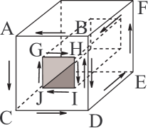
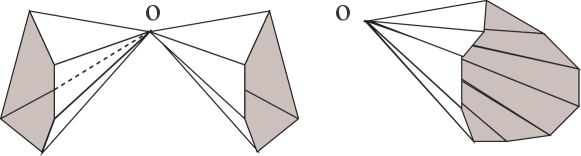
(a) (b)

Figure 2.19: Orientation of loops in the RES (a) and a pair of different fans of ten triangles (b). Both fans implies that vertex $o$ has twenty vertex uses in its radial–edge representation. In both situations the twenty uses are linked in a unique list.

This problem is properly adressed by the tri-ciclic cusp data structure [59] that introduce disks around vertices to group vertex uses (see Section 2.2.4).

The radial–edge data structure has several slightly different implementations. Some of them are part of commercial packages (e.g. Smlib [110]). Weiler itself at Autodesk revised the original data structure to take care of the above mentioned problem of isolated non-manifold vertices [128]. In this review we found convenient to describe the radial–edge data structure implemented in the NMG package in BRL-CAD [10] (as described in [99]). Thus, in Figure 2.18 we reported all arrows for mutual references inserted in nodes that implements the radial–edge topological entities. Arrow tips labeled with a star denotes partial relations. For a partial relation just one reference is stored even if the elements to be referenced are many. Other elements will be recovered using alternative paths in this diagram.

Arrows labeled with integers in Figures 2.18 and 2.20 denotes relation between objects implementing topological entities. We will describe briefly the meaning of all these relations:

EUs for an edge are linked pairwise (by relation 2) and are organized into two cycles of edge uses. More in particular:

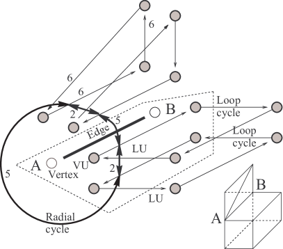
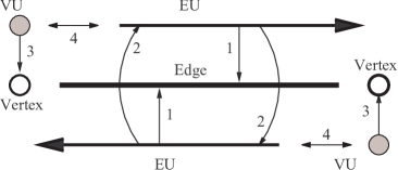
(a) (b)

Figure 2.20: An example of radial and loop cycles in the fragment of the radial–edge around edge AB for the complex in the right lower corner of figure (a) and an example (b) of relations for a pair of EU associated to the use of an edge by a certain face. Figure (b) is the detail of the framed portion of figure (a) (both adapted from [99])

• EUs are then organized into two cycles: One for all EUs participating to a LU (this is what is called the loop cycle (6)) and one for all EUs of a given edge. This is what we called the radial cycle (i.e. 2-5 cycle) (see Figure 2.20 (a)).

• A binary relationship (2) is defined for the pair of EUs for the same edge that corresponds to the two possible orientations of an adjacent face (see Figure 2.20 (b));

The uses reference their parent in the RES hierarchy, thus LU reference L (8), FU reference F (9), EU reference E (1), The inverse relations for the above three relations are all stored as partial relations. A VU reference (3) its parent V and the inverse relation is stored completely since all VU for a certain vertex are linked in a list (7). FUs comes in pairs for each face and corresponding pairs of FUs are related by relation 13. Similarly LUs comes in pairs, two for each loop, and corresponding pairs of LUs are related by relation 14. A single bounding LU correspond to each FU in the bijection 15. For non-simply connected faces several LU are linked in a list (not shown in the diagram of Figure 2.18) and the FU points to the head of this list. A LU reference (16) one of its EUs and each EU reference (16) the LU to which it belongs. All FUs reference (10) the shell they belongs to and a shell reference one of these FU, others are linked in a list (not shown in the diagram of Figure 2.18). All shells reference (11) the region they bound to and a region reference one of these shells, others are linked in a list (not shown in the diagram of Figure 2.18).

The evaluation of space requirements for this representation is possible if we assume something about the nature of the cellular subdivision of the model. Following statistical assumptions, in [73], a storage requirement of $4.41$ times the space needed by the winged–edge is reported in [73]. This is evaluated assuming that the RES is used to encode the boundary of a single shell manifold solid.

We evaluate here the number of references needed to encode a simplicial subdivision of a regular 3-complex. To this aim we first list all the instances of radial–edge elements we need to encode a tetrahedron and report between parenthesis the number of references required by each instance. This is evaluated as the number of arrows coming out of the corresponding object in Figure 2.18. Thus, to model a tetrahedral cell we need one region (1), one shell (2), a list of four FU (4 references for the list and 3 references for each FU), four LU (4). For each triangle we need three EU (7) and three VU (3). This sums to 155 references. Note that we omitted space needed for faces (F), loops (L), edges (E) and vertices (V) that will add one reference for each of these entities. If one is forced to encode a tetrahedralization with this scheme the storage requirement will be 155t+2f+e+v. We count two references for each face since we have to introduce one loop for each face.

The Tri-cyclic cusp Data Structure

This data structure [59] is similar to the RES. Variations are introduced to correct a RES limitation. Some topological elements are added, some elements in the RES are renamed and some names of the RES are used to denote a different element with some awkward overlapping of names. In Figure 2.21 we report a fragment of a tri–cyclic cusp data structure for the complex in the lower left corner of this figure.

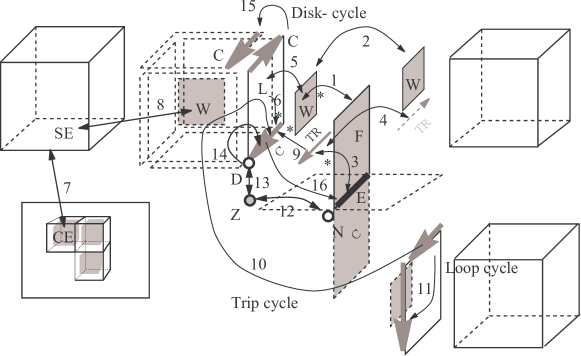
Figure 2.21: Elements in a fragment of a tri–cyclic cusp data structure for the complex in the lower left corner. Arrows represent a relation between topological entities described in [59].

In the following description of the tri-ciclic data structure we report in parenthesis the labels used in Figure 2.21 to denote topological elements in the data structure.

A first thing to note is that, the Loop (L) of the tri-ciclic data structure actually plays the role of the loop-use in the RES while, in the tri-ciclic data structure, the loop node of the RES is omitted.

A cell (CE) in this cellular subdivision is delimited by one or more seals (SE) each seal being an orientable manifold surface. In this data structure each face is represented by two distinct element one for each oriented face. Oriented faces are called walls (W). Walls corresponds to face-uses in the RES. Thus each seal is represented by a collection of walls with coherent orientation. More than one seal is used to model cells with cavities.

This data-structure is an improvement with respect to the radial–edge since it orders edges around a vertex into separate lists whenever several distinct fans are incident to a vertex. Each separate fan is called a disk and the circular list of edges that belongs to a fan is called a disk cycle. Disks partition the 3D space around a vertex into zones.

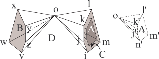
Figure 2.22: A example illustrating the zone concept in the tri–cyclic cusp representation

See for instance the situation of vertex $o$ in Figure 2.22. In this figure let us consider the three cones from $o$ to the perimeter of the three polygons $xyzvw$, $ijklm$ and $i^{\prime}j^{\prime}k^{\prime}l^{\prime}m^{\prime}$. In the situation of Figure 2.22 let us imagine that we have six disks, two coincident disks for each cone. Two disks are associated with each $1$-connected component in a vertex star. The three components (cones) partition the neighborhood of vertex $o$ into three finite zones, denoted by $A$, $B$, $C$, and an unbound zone $D$. Each zone is bound by two cones. Thus we can partition the six disks into four disjoint pairs that are the boundaries for the four zones.

In the tri-ciclic data structure each of the triangles in Figure 2.22 is represented by two distinct oriented faces (i.e. walls) that correspond to face-uses in the RES. Edges delimiting each triangle are duplicated for each wall. These duplicated edges are called cusps (C). Cusps plays the role of edge-uses in the RES. Thus, in the tri-ciclic data structure, each side of each cone is actually represented by a distinct structure given by a list of cusps. This list of cusps is called a disk cycle. Each cycle defines the topological entity we called the disk. To model this topological entity a specific topological element called disk (D) is introduced in the data structure.

As we have seen in Figure 2.22 disks partition the space around a vertex into zones. To model this topological entity another specific topological element called zone (Z) is introduced in the data structure. Each zone is delimited by one or more disks and note that we can have zones delimited by more than two disks. An unbound zone might be delimited by just one disk. The entity representing the zone reference these disks and the vertex at the apex of each disk. For each pair of zones sharing a boundary we have two disks, one for each side of the common boundary. Therefore each disk delimits just one and not two zones.

Thus in the tri-ciclic cusp data structure a vertex is modeled by a node (N) that references a list of zones (Z) each of which is delimited (and reference) two disk cycles represented through disks (D).

A cusp (C) is used to model a number of different topological entities. Cusps can represent dangling edges or isolated vertices. However, usually a cusp models an edge adjacent to a wall. In this case the cusp participate to the above mentioned disk cycle. Cusps are inserted into other two cycles. A second cycle, called the loop cycle links cusps that delimit a wall. A third cycle, called the trip cycle. links all of cusps that have the same orientation and are associated to the same edge. The name of the representation comes from the fact that there are three cyclic relations between cusps: the disk cycle, the loops cycle and the trip cycle. The loop cycle links cusps that delimit a wall while adjacency between walls is defined grouping adjacent edges (i.e cusps) into a cycle called the trip cycle. Finally all cusps adjacent to the same vertex are grouped into cycles that defines vertex disks.

Finally we analyze the relations between the topological elements in this data structure using integer labels of Figure 2.21. A cell in a tri-ciclic data structure reference one or more delimiting seals (7). Each seal reference (8) the collection of walls with coherent orientation that defines the seal.

A face reference (through the partial relation 1) two walls (W) representing the two possible orientations for a face. Each wall must reference its parent face (1) and its opposite wall (2).

Edges reference (through the partial relation 3) two trips (TR) representing the two possible orientations for an edge. Each trip must reference its parent edge (3) and its opposite trip (4). The trip reference (9) one of the cusps in the associated trip cycle (10). Each cusp reference the corresponding edge (16).

A wall is bounded by one or more loop cycles (11). Thus a wall must reference (5) one or more loops. Each loop reference (5) the wall it belongs to. A loop reference (6) one of the cusps in the associated loop cycle.

A node (N) (i.e. a vertex) reference (12) the set of zones its neighborhood is divided into. A zone reference (12) its parent node and its disks (13). Each disk reference (13) the zone it bounds. Disks reference (14) one of the cusps in the associated disk cycle (15).

The evaluation of space requirements for this representation heavily depends on the kind of cellular subdivision adopted We evaluate here the number of references needed to encode a a simplicial subdivision of a tetrahedron. To this aim we list all the instances of tri–ciclic elements we need to encode the tetrahedron and report between parenthesis the number of references required by each instance. This is evaluated as the number of arrows coming out of each object in Figure 2.21. To model a tetrahedral cell we need one cell (1), one seal (1), a list of four triangular walls (4 references for the list and 3 references for each W), four loops (L) (2). For each triangular wall we need three cusps (4). Finally each vertex of the tetrahedron must be associated with a disk. Thus we need four disks (2) and four zones (2). One more pointer is needed for each zone to build a list of zones. This sums to 94 references. Note that we omit space needed for faces (F), edges (E) and nodes (N) that will add one reference for each of these entites. If one is forced to encode a tetrahedralization with this scheme the storage requirement will be 94t+f+e+v.

The Partial Entity Data Structure

The partial entity data structure (PES) [73] is a reduced version of the RES obtained by neglecting loop-uses. Thus, for each face, we have a single loop (L). In the face-uses, that here are called partial faces (PF), is stored a flag that allows to compare the orientation of the loop with the orientation of the partial face. In Figure 2.23 we list all entites in the PES. Large characters are used to denote entites that differ from those in the RES.

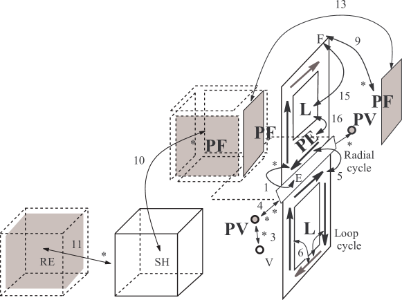
Figure 2.23: Topological entities in the partial entity data structure

Loops are obtained as doubly-linked cycles of entities called partial edges. Partial edges plays the role of edge uses in RES but, with respect to  them, we have just a partial edge for each face adjacent to a given edge. On the contrary, in the RES, we have to introduce an edge use for each (boundary of a) cell adjacent to a given edge.

We will describe briefly the meaning of all the relations in Figure 2.23. We use non-contiguous integers to label relations. This is to keep labeling used for RES whenever possible. We have used labels 1,3,4,5,6,9,10,11,13,15,16 to highlight the fact that the corresponding relations in the RES have a similar meaning.

A region (i.e. a cell) is bounded by one or more cells. All shells reference (11) the region they bound to and a region reference one of these shells, others are linked in a list (not shown in the diagram of Figure 2.23). All PFs reference (10) the shell they belongs to and a shell reference one of these PF, others are linked in a list (not shown in the diagram of Figure 2.23).

PEs for an edge are organized into two cycles implemented with doubly-linked lists. One cycle is for all PEs participating to a loop (this is what is called the loop cycle (6)) and one for all PEs of a given edge. This is called the radial cycle (i.e. 5 cycle).

Partial elements reference their non-partial counterpart in the PES hierarchy, thus PE reference E (1), PF reference F (9), PV reference V (3). The inverse relations for the above three relations are all stored as partial relations.

PFs comes in pairs, two for each face, and corresponding pairs of PEs are related by relation 13. A single bounding L correspond to each F in the bijection 15. For non-simply connected faces several L are linked in a list (not shown in the diagram of Figure 2.23) and the F points to the head of this list. A loop L reference (16) one of its PEs and each PE reference (16) the loop it belongs to. A PV points an incident edge E and E points the two PV one for each endpoint (4).

The evaluation of space requirements for this representation heavily depends on the kind of cellular subdivision adopted. Following statistical assumptions the PES is assigned in [73] a storage requirement of $2.17$ times the space needed by the winged–edge. This is evaluated assuming that we have to encode the boundary of a manifold solid enclosed by a single shell. Under these assumptions the RES is more expensive with respect to PES by a factor 2.03.

Alternatively to this analysis we evaluate here the number of references needed to encode a simplicial subdivision of a tetrahedron. To this aim we list all the instances of PES classes needed to encode a tetrahedron and report between parenthesis the number of references required by each instance. This is evaluated as the number of arrows coming out of each object in Figure 2.23. To model a tetrahedral cell we need one cell (1), one seal (1), a list of four triangular PF (4 references for the list and 2 references for each PF), four loops (L) (2). For each triangular PF we need three PE (5). Finally each vertex of the tetrahedron must be associated to a PV. Thus we need four PV (2). One more pointer is needed for each PV to build a list of PV. Note that references for each loop and PEs are 17 per face and must be counted just once for each face. In this way this structure saves a lot of space with respect to  the RES. The remaining references sums to 27 references for each tetrahedron. Note that we omit space needed for faces (F), edges (E) and vertices (V) that will add $2f+2e+v$ references. If one is forced to encode a tetrahedralization with this scheme the storage requirement will be 27t+19f+2e+v. If we assume a manifold tetrahedralization we can say that $4t\leq 2f$. If we forget boundaries and assume and we get an occupation of 65 references for each tetrahedron that is less than half of the space needed by the RES.

2.2.5 Conclusions

We have reviewed several approaches to model realizable non-manifolds and for each approach we have computed the storage requirement required to encode a simplicial subdivision with $t$ tetrahedra, $f$ faces, $e$ edges and $v$ vertices. The results of this analysis are summarized in Table 2.3.

Modeling Data Structure		storage requirement
1	Radial Edge	$155t+2f+e+v$
2	Tri-Cyclic Cusps	$94t+f+e+v$
3	Partial Entity	$27t+19f+2e+v$

Table 2.3: Storage cost for non-manifold data structures

We already reported a ratio of 2.01 between storage requirement of RES and PES following results in [73]. It can be proven that the storage requirement of the Tri-Cyclic Cusp data structure is intermediate between storage requirement of RES and PES. Thus the storage requirement of PES is the best in this class and still its storage requirement, according to [73], is at least twice the storage requirement needed by the standard data structures for manifold surfaces (e.g. the winged-edge).

2.3 Decomposition of non-manifold surfaces and solids

The idea of representing polyhedra through its decomposition is already present in literature since 1984. The original formulation of the problem is contained in papers about notch cutting [28]. However in this area of research the emphasis was on the decomposition of a generic solid polyhedron ${\mathcal{P}}$ into convex polyhedra. The non-manifold edges and vertices in the boundary of the polyhedron ${\mathcal{P}}$ were called special notches and their removal is performed using a geometric decision procedure [11]. This can lead to a decomposition based on the geometry that might not be satisfactory in general.

Depending on the surface normal we use, the two boxes sharing an edge in Figure 2.24 (a) might be decomposed into two boxes (Figure 2.24 (b)) or into a single volume obtained making the two boxes communicate through the common edge split in two (Figure 2.24 (c)). This is clearly pointed out in [91] from which we quote the examples in Figure 2.24

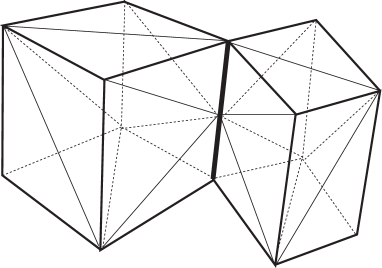
(a)

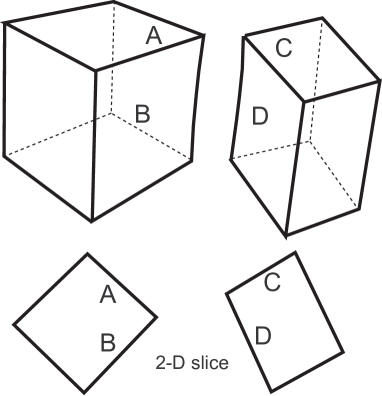
(b)

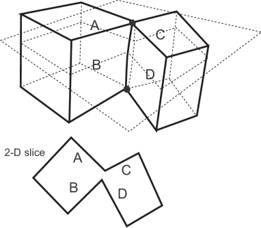
(c)

Figure 2.24: Ambiguities in decomposition of non-manifold solids. A non-manifold solid (a) and two possible patterns for the underlying non-manifold data structure (b) and (c) (adapted from [92])

Nevertheless, several topological modeling approaches assumes that a decomposition procedure for $2$-complexes is available and propose a modeling approach based on the decomposition of the boundary of the solid to be modeled.

2.3.1 TCD Two-manifold Cell Decomposition Graph

In [46] the decomposition of [11] is taken as starting point. Thus a decomposition of the original non-manifold solid is assumed. This decomposition is assumed to provide manifold components by duplicating edges and vertices at special notches.

Each component of the decomposition is taken then as a separate cell. Thus cells are the interior of orientable closed $2$-manifolds. These cells are represented through their boundary that in turn is modeled with a standard cellular decomposition for 2-manifolds. Edges and vertices that are copies of special notches are then grouped together using an hypergraph called the two-manifold cell decomposition graph (TCD). In the original paper access primitives to the representation are not presented, nor it is detailed how to build the proposed data structure using decomposition results. The paper contained a claim that a set of two Euler operators and their inverses is sufficient to implement needed primitives for a non-manifold solid modeler.

2.3.2 The non-manifold spine representation

In [37] a non-manifold solid is proven to be equal to the limit (with respect to a certain metric) of a sequence of manifold solids. This theoretical result is used to prove that extending the usual set of Euler operators one can define non-manifold solids through these sequences. Obviously the extended operators act on a sequence of manifold solids and returns a sequence of manifold solids. However, it can be proven that both these sequences and the operators admit a finite representation. To prove this result this paper presents a data structure for non-manifold solids. In this data structure the non-manifold solid is represented through a set of manifold solids together with the set of all non-manifold points. In a non-manifold solid this set is a graph called the non-manifold spine. In the manifold solids are inserted finite combinatorial objects called infinitesimal faces whose semantics is the sequence of faces needed to approximate the non-manifold r-set. Infinitesimal faces behaves as ordinary faces within approximating manifold solids. Infinitesimal faces are involved in an adjacency relations with the elements of the manifold spine. These adjacency are collectively stored within an hash table. We will call the manifold spine representation the combination of these four components: the manifold spine, the infinitesimal faces, the set of manifold solids with infinitesimal faces and the encoding of the adjacency relations between the spine and the infinitesimal faces. Completeness of the set of extended Euler operators is proven in two steps. First it is proven that the manifold spine representation can model all approximating sequences of manifold solids. Next it is proven that introduced operators are designed to build all valid instances of this representation. In this paper it is not detailed how to build the proposed decomposition of the non-manifold solid. However it is proven that it is possible to build the proposed data structure with the extended Euler operators introduced by this scheme. Higher level primitives, like a sweep operator, are implemented using this set of Euler operators. However, is still responsibility of the user to give the correct sequence of Euler operations that can build a certain non-manifold solid.

2.3.3 Cutting and Stitching

Cutting and stitching is presented in a pair of works that do not address directly the non-manifold modeling problem. On the contrary at least one of them [56] tries to avoid non-manifoldness by converting a non-manifold surface into a manifold surface. The work consider a more general class of non-manifolds since it do not assume to work with solids and do not use the notion of interior. No user supplied modeling is assumed and the topological input data are assumed to be available in a raw list of faces. The conversion is performed in a two step process. In a first step the original complex is decomposed. Two decomposition algorithms are presented. The algorithms presented in this thesis can be considered as a dimension independent extension of these algorithms to non regular complexes of arbitrary dimension. Further discussion on this relation is presented in the last section of this chapter. The cutting algorithm proposed in [56] is shown to have complexity proportional to the number of (non-manifold) marked edges times times the largest number of corners in a vertex star.

In a second step the result of cutting is reprocessed in order to stitch together edges that were cut in the previous step. This action is called a stitching. This second step must produce a manifold surface. A particular manifold stitch is produced using greedy strategies. Two criteria are proposed. One is to attempts to maximize the number of edges that stitches together (called a maximal length stitch). Another algorithm attempts to maximize the number of vertices that stitches together. (called a maximal size stitch). Two strategies are presented. The first strategy stitches only edges or vertices that were previously cut by the cutting algorithm. In a second strategy this constraint is removed and stitching is promoted using geometric proximity.

The two algorithms are used to convert a non-manifold surface into a manifold surface that can be used as input to simplification algorithms for manifolds. The result of the conversion is also fed to a compression algorithm for manifolds [122] based on topological surgery. The compressed surface will have the same geometric realization of the original non-manifold complex but will retain the combinatorial structure of the decomposed complex. A later work [55] extends the topological surgery compression scheme to handle directly the non-manifold surface and deliver a compressed version that preserves the combinatorial structure of the non-manifold surface. Non-manifold compression is performed by cutting first along non-manifold points following the cutting process in [55]. Then parts are compressed using topological surgery. The non-manifold structure is compressed adding the encoding for the inversion of the cutting process through a set of stitching instructions. Note that cutting in [56] is limited to regular $2$-complexes. The proposed cutting algorithm is shown to have complexity proportional to the number of (non-manifold) marked edges times the largest number of marked edges times the largest number of corners in a vertex star. It is easy to exhibit simplicial subdivisions of non-manifold surfaces where using this statement we can predict a processing time that is quadratic with respect to the number of faces. To obtain our dimension independent extension algorithm we simply restated the algorithms presented in [56] in a recursive style. The result of cutting is referred to be the manifold with the maximum number of vertices and the maximum number of components that cuts through the singular edges and vertices and nowhere else.

2.3.4 Matchmaker

Finally, Matchmaker is an algorithm, presented in [114], that is especially conceived to decompose the boundary of r-sets (or even a 2-complex) into a set of manifold surfaces. This approach, although limited to non-manifold 2-complexes, attempts to minimize the number of vertex replications introduced by the decomposition process. In a situation like that of Figure 2.25 (a)

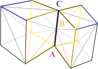
(a)

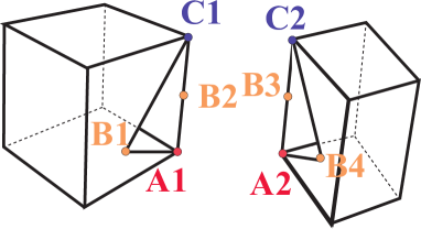
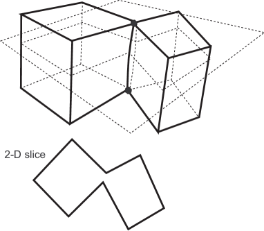
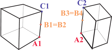
(b) (c) (d)

Figure 2.25: Matchmaker and the decomposition of non-manifold solids. A non-manifold solid (a) and three possible decompositions: Matchmaker (c) the Canonical Decomposition (in this thesis) (b) and another option as in [91](d)

Matchmaker turns the original solid (a) into a manifold model as in (c) without introducing vertices duplication as in (d). The resulting model is manifold because of the geometric embedding. In the embedding Matchmaker assumes that edges can be duplicated introducing a couple of infinitesimally curved edges. The two cubes becomes a single volume obtained making the two boxes communicate through the common edge split in two. The authors calls this kind of surface edge manifold. As they say: if these edges were bent by an infinitely small amount in the appropriate direction, the resulting shape would either be manifold or would have only isolated non-manifold vertices. We say that the resulting model is edge-manifold. The algorithm introduces duplication for isolated non-manifold vertices and obtain a manifold embedding for the original model. Going on with this idea the algorithm also corrects self intersections in the geometric model. The whole approach is different from the one presented in this thesis. Indeed, with Matchmaker, in the combinatorial structure of the decomposed model, the common edge in Figure 2.25 (a) remains adjacent to four faces and manifoldness is obtained in the embedding by curving edges. A second distinction is about the type of algorithm. With Matchmaker the output depends on some greedy choices that may result in vertex replications that could be avoided. Indeed we try to devise a decomposition that is the most general among possible decompositions. As a consequence we introduce more vertex replication. In the case of Figure 2.25 (a) our decomposition will go recursively to decompose the colored 1-complexes of Figure 2.25 (a) and count their connected components. Thus for A we decompose the graph in red and count two connected components. The same happens for C in blue. The decomposition for B accounts for four components (the four Cs in yellow). Thus we introduce two copies for A and C, and four copies for B. The resulting decomposition is in (b) and is the most general since both cases in (c) and (d) can be obtained by further stitching. Yet is not too general cutting only at non-manifold edges. We felt that all the details about how to define italicized words require the framework of combinatorial topology.

2.4 A rationale for a combinatorial approach

In this thesis we basically present a dimension independent decomposition scheme for non-manifolds and a related data structure. In this section we give motivation for the role we reserved, in this thesis, to combinatorial topology (a.k.a. piecewise linear topology or PL-topology). To this aim we report basic negative results that characterize the incomplete relation between combinatorial and point set topology in higher dimension. This incomplete relation must be taken into account when choosing a theoretical framework for a dimension independent formulation.

2.4.1 Motivations

For the particular study we carried out in this thesis we felt uneasy to develop this study in a geometric framework and, as we have reported, it is not essentially mandatory to embed the theoretical framework in ${\rm I\kern-1.99997ptR}^{k}$. Furthermore all results in this thesis do not mention the particular embedding. This is the reason why we found nice and profitable to have a completely combinatorial presentation. Finally, in the context of this thesis, the value of dimension independent results obtained in the geometric settlement (i.e. ${\rm I\kern-1.99997ptR}^{k}$) is questionable. The value of these results is based on the shaking ground of the incomplete relationship between point set and combinatorial topology. To show that a combinatorial approach is essentially due we will outline, in this section, classic negative results about the relation between point set and combinatorial topology.

However, before starting this review of related results in combinatorial topology, we try to explain why they are related with this work. We try to do this with an example.

With the following example we want to show that there are reasonable clues that it is not feasible to investigate the subject of this thesis in ${\rm I\kern-1.99997ptR}^{k}$ and then translate back theoretical results from ${\rm I\kern-1.99997ptR}^{k}$ into the language of cellular decompositions.

To build such an example we take one of the main results of this thesis and see a possible similar result formulated in the language of point set topology. In particular, in this example, we assume that we have derived (somehow) this ”continuous” formulation and enlight the difficulties that are behind a translation of the continuous result into a result for cellular (or simplicial) subdivisions.

One of the central results in this thesis is that there exist a unique maximal decomposition (denoted by $\nabla\cdot{\Omega}$) of a given simplicial $d$-complex $\Omega$ obtained cutting $\Omega$ only at non-manifold simplices. Thus the continuous analogue of this result might state that, for a given polyhedron $P$ in ${\rm I\kern-1.99997ptR}^{k}$, there is a unique, up to homeomorphism, maximally decomposed polyhedron $\nabla\cdot{P}$ that can be mapped into $P$ by a continuous function such that the common image of two distinct points in $\nabla\cdot{P}$ is always a point that has not a neighborhood homeomorphic to ${\rm I\kern-1.99997ptR}^{k}$. By maximally decomposed here we mean that there is not another polyhedron $P^{\prime}$ with the above characteristics and such that $\nabla\cdot{P}$ is the continuous image of $P^{\prime}$.

Let us forget the problem of producing a correct ”discrete” theorem that exploits completely this (hypothetical) result and let us just mention the fact that this continuous version seems a quite hard result to prove. Surely a simple consequence of such a result is that, given an abstract simplicial complex $\Omega$, ve must define the discrete decomposition $\nabla\cdot{\Omega}$ as any triangulation of the decomposition $\nabla\cdot{P(\Omega)}$ of a geometric realization $P(\Omega)$ of $\Omega$. This definition is actually faulty in higher dimension since an arbitrary triangulation of a manifold need not to be a combinatorial manifold. This is one of the classic negative results [40] we will mention in the review of the following section. Thus, not all points that are manifold points in $\nabla\cdot{P(\Omega)}$ must be manifold vertices in $\nabla\cdot{\Omega}$ and consequently the class of non-manifold singularities that are removed in $\nabla\cdot{\Omega}$ is not clearly identified. Thus, we found interesting to review, in this section, all mathematical results that characterize the incomplete relation between ”continuous” topological concepts and their ”discrete” analogue.

2.4.2 Topological and Combinatorial Manifolds

Manifolds are usually introduced by a rather geometric definition that actually gives the notion of topological $d$-manifolds. A topological $d$-manifolds is a topological subspace of some Euclidean space such that every point has an open neighborhood that is homeomorphic to ${\rm I\kern-1.99997ptR}^{d}$. However, often a theoretical model closer to the computerized representation is needed. Therefore, one it is forced to modify this definition and introduce an analogous combinatorial definition that views manifolds as a collection of related discrete entities (e.g. $d$-simplices).

A first step in this direction is to define a slightly different class of objects called triangulated manifolds. Triangulated manifolds are defined as topological manifolds that are also geometric simplicial complexes i.e. collection of discrete entities (triangles or tetrahedra) glued together. A topological manifold is triangulable iff it is equivalent (i.e. homeomorphic) to a triangulated manifold. Triangulable $d$-manifolds are a proper subclass of topological $d$-manifolds. In fact there are manifolds that do not have a triangulated equivalent. This is already true for $d=4$ (see [4] that combines results by Freedman [48, 49] and classical Casson results [18] Pg. 5).

If we restrict our attention to the subclass of geometric simplicial complex it can be proved (see [38] p. 2 for instance) that a simplicial complex is a triangulated $d$-manifold iff the star of simplices around each vertex (see Definition 3.2.2) is homeomorphic to ${\rm I\kern-1.99997ptR}^{d}$. Equivalently, we can say that a simplicial complex is a $d$-manifold iff the link of each vertex (i.e. , in manifolds, the boundary of the vertex star) is homeomorphic to the $(d-1)$-sphere. Therefore, to recognize $d$-manifolds we must be able to recognize the equivalence of a simplicial $(d-1)$-complex with a $(d-1)$-sphere.

To have a combinatorial analogue of manifoldneess definition one must turn from vertex link equivalence based on homeomorphism to PL-equivalence based on piecewise linear homeomorphism (PL-homeomorphism). PL-equivalence proves to be truly combinatorial (see [118] p. 520) and at least semi-decidable. In fact, two $d$-dimensional simplicial complexes are PL-homeomorphic iff they are stellar equivalent. and simplicial complexes are stellar equivalent if they can be transformed into a common refinement by a finite sequence of discrete operations, called starring operations. Each starring operation is a finite operation that modifies the combinatorial structure of the complex. Therefore, stellar equivalence is at least a semi-decidable relation (see [74] for a survey on stellar and bistellar equivalence).

The adoption of PL-equivalence, also called combinatorial equivalence leads to a first definition of the closed combinatorial $d$-manifold, that is: A closed combinatorial $d$-manifold is a triangulated manifold where every point has a link that is piece-wise linearly homeomorphic (PL-homeomorphic) to the $(d-1)$-sphere.

This definition of combinatorial equivalence is recognized as the best discrete analogue of the topological definition of homeomorphism and still the analogy is known to be unsatisfactory. In fact, in general, it is false that two $d$-complexes that are homeomorphic must be PL-homeomorphic (PL-equivalent). The italicized assumption is called Steinitz’s Hauptvermutung and it was the basic assumption behind combinatorial topology. This assumption clearly legitimate the claim that we can study some properties of topological spaces w.l.o.g. by studying properties of complexes.

This assumption is known to be true for $d$-complexes for $d\leq 2$ [104] and for $d=3$ [94] and is known to be false in general. In fact Milnor [93] provided the first example of a pair of non-manifold $7$-complexes that have homeomorphic geometric realizations and yet that are not PL-equivalent. Besides Milnor counterexample for $d=7$ the Hauptvermutung is an open problem for $d\geq 4$.

Obviously PL-homeomorphism is semi-decidable via stellar equivalence, however, this do not implies that the definition we have given for $d$-manifolds is still satisfactory. In fact, we can use semi-decidable stellar equivalence to see if the link of each vertex is PL-homeomorphic to a particular triangulation of the $(d-1)$-sphere. Thus to validate a $d$-manifold we must select a particular reference simplicial complex for the $(d-1)$-sphere and then check every vertex link. Thus, in the end the best discrete analogue of the definition of the closed topological manifold is the following: A closed combinatorial $d$-manifold is a triangulated manifold where every point has a link that is piece-wise linearly homeomorphic (PL-homeomorphic) to the $(d-1)$-simplex

However the results of this link checking should not depend on the particular triangulation selected for the $(d-1)$-sphere. This is possible iff all triangulations of the $d$-sphere are PL-equivalent. The correctness of this assumption is actually an open problem for $4$-spheres. On the other hand it has been proved that, for $d\neq 4$, the standard $d$-simplex is a unique reference structure for all triangulations of $d$-sphere that are also a combinatorial manifold (see [94] for $d\leq 3$ and [68] for $d\geq 5$). However, already for $d=5$, it has been discovered an example of a triangulable $5$-sphere that is triangulable into a complex that is not a combinatorial manifold in the sense of the definition above [40].

Thus, as far as we are concerned in this thesis, for $d\geq 4$ it is not that obvious tha we can translate a results on topological manifoldness to a similar result in term of combinatorial manifoldness. We feel that this suggest to develop a dimension independent study of this kind with an approach that makes little or no reference to concepts from point set topology. Even if we stay in the combinatorial domain, still we have to comply with some other limitations when we are developing a dimension independent approach. We briefly report them here since an easy consequence of these results is that a decomposition into manifold parts is not always possible in higher dimension (see Property 8.3.1).

2.4.3 Manifold limitations in higher dimension

We have seen that the Hauptvermutung is false and thus combinatorial equivalence is less powerful that topological equivalence. However, even if we accept to work with combinatorial equivalence still we have that for $d\geq 4$ combinatorial equivalence is only semi-decidable. This is a consequence of a result by Markov [88]. This result states that there exist $4$-complex $\Omega_{0}$ such that it is impossible to decide, for any other complex $\Omega$, if $\Omega_{0}$ and $\Omega$ are combinatorially equivalent.

Following Markov approach Novikov proved [125] that there exist a combinatorial $d$-manifold $M_{d}$, for any $d\geq 5$, s.t. we cannot decide whether $M_{d}$ is a $d$-sphere or not. Novikov, following a technique that was already in Markov paper [88], proves this result (as reported in [125]) showing that the problem of recognizing a $d$-sphere for $d\geq 5$ implies the problem of recognizing a trivial group in a finite sequence of finitely generated groups. It is known [1] that this problem, in turn, implies the Halting Problem. The relation between the recognizability of the $d$-sphere and the halting problem is unfolded, for instance, in [100]. These results, in turn, impair the possibility of recognizing combinatorial $d$-manifolds for $d\geq 6$ (see Theorem 3.5.3). An easy consequence of this is that a decomposition into manifold parts is not always possible in higher dimension (see Property 8.3.1).

2.4.4 Summary

In the end, the best founded definition for combinatorial $d$-manifolds requires the link of every vertex to be PL-homeomorphic to the boundary standard $d$-simplex. This definition is truly combinatorial since PL-homeomorphism is at least semi-decidable via stellar equivalence. Combinatorial $d$-manifolds then are a proper subclass of triangulated $d$-manifolds already for $d=5$. In fact there exist a triangulable $5$-sphere that is not triangulable as a combinatorial manifold [40].

This short review of the fundamental problems in the definition of $d$-manifolds proves that the above definition of combinatorial manifold is, up to now, the best combinatorial analogue of the local euclidean condition required by topological manifolds.

Nevertheless, some problems remains and we can say that things works completely fine only in dimension lower than three. For $d\leq 3$ all topological $d$-manifolds are triangulable [13, 94] homeomorphism and PL-homeomorphism are equivalent (i.e. the Hauptvermutung is true), the $d$-sphere has a unique structure (i.e. the boundary of the standard $(d+1)$-simplex) and, for $d\leq 3$, the $d$-sphere is algorithmically recognizable [123]. However the classification of three manifolds is still an open problem.

For $d=4$ there exist a $4$-manifold not triangulable and it is unknown if the $4$-sphere has a unique structure or whether it is recognizable. For $d\geq 4$ the Hauptvermutung is an open problem and both homeomorphism and PL-homeomorphism between $d$-manifolds are not decidable. For $d\geq 5$ the $d$-spheres that are triangulable as combinatorial $d$-manifolds has a unique structure, however already for $d=5$, we find a triangulable $5$-sphere that is not triangulable as a combinatorial manifold [40]. For $d\geq 4$ $d$-manifolds can not be classified [88] and for $d\geq 5$ the the $d$-sphere is not recognizable [125].

All these limitations, especially those in the classification of $d$-manifolds, impair the possibility of using them as building blocks in the decomposition of non-manifolds. Furthermore, for these negative results it is not possible to build a satisfactory relation between results derived in ${\rm I\kern-1.99997ptR}^{k}$, using point set topology definitions and their combinatorial counterpart. For this reason a purely combinatorial approach has been adopted in this thesis.

2.5 Conclusions

In this section we collect some notes about the relation between the results in this thesis and reviewed related works.

2.5.1 Representation domain for cell complexes

A first relation that might be considered is the relation of the results in this thesis with several modeling approaches presented in Section 2.2.4. If we omit approaches for $2$-manifolds all other approaches pretend to model cell complexes where only two $3$-cells are incident to any given $2$-cells. In general cells are defined by shells of face uses or similar entities. Face uses comes in pairs for each face, Therefore there is no way to model a non-pseudomanifold $3$-complex made up, for instance, by three tetrahedra sharing the same triangle. A similar limitation is present also in dimension independent modeling schemes. Modeling schemes artificially constrain their domain of representation to some well known topological class but the problem of characterizing the domain of the representation is still open. More precisely we cannot say what is exactly the subclass of the topological subspace of ${\rm I\kern-1.99997ptR}^{n}$ that can be represented by a uniformly dimensional cellular subdivision such that a $(d-1)$-cell is always adjacent at most to two $d$-cells.

In this thesis we will study this domain for simplicial subdivisions. We will show that the representation domain of the winged representation is, the set of Quasi-manifolds defined by Lienhardt [80] (see Property 7.5.1 and Definition 7.5.2). Next we will give a characterization of this class of complexes in term of local topological properties. It is well konwn that quasi-manifold surfaces are ordinary $2$-manifold surfaces and in dimension three of higher quasi-manifold are a proper superset of manifolds.

In this thesis, in order to study the decomposition problem, a different point of view is investigated assuming an operational view of the winged representation. In fact we can give the winged representation an operational interpretation considering the adjacency function ${\mathcal{A}}$ as a set of gluing instructions that tells how to stitch together $d$-simplices gluing them at $(d-1)$-faces. Obviously we constrain gluing instructions not to glue together more than two $d$-simplices at time. However note that a gluing between two $d$-simplices might induce gluings between other $d$-simplices. Note that this view is exactly what we have in mind when we want to find out what is represented by a given instance of a certain modeling data structure stored by some program in some computer memory.

Surprisingly enough the representation domain for this operational view is not the same of the original representation domain for the winged representation. We show that by this gluing process we generate a class of objects, we called Initial-Quasi-Manifold, that are a proper superset of Quasi-manifold. We will give a characterization of this class of complexes in term of local topological properties (see Property 7.5.1 and Definition 7.5.2). The most surprising fact coming from this analysis is that non-pseudomanifold complexes can be built with this operational view. Thus a non-pseudomanifold $3$-complex can be stored in most data structures for non-manifold solids even if this kind of non-pseudomanifoldness is not directly represented by these data structures. In other words we found out that a set of gluing instructions that do not to glue together more than two $3$-simplices at time might generate a tetrahedralization where three tetrahedra must be incident to the same, non-pseudomanifold triangle (see Example 7.4.2).

2.5.2 Extension of the winged representation to the non-manifold domain

In section 2.2.4 we presented three modeling approaches that can model cellular subdivisions of realizable non-manifolds. These approaches are reviewed and presented stressing the fact that they all can be understood as small variations around the original scheme present in the radial-edge data structure. On the other hand, in Chapter 9 we define a data structure that represents a strong departure from this model. In this we see a strong relation with the winged representation (see Section 2.2.3) because our data structure is essentially an extended version of the winged representation that is capable of handling complexes that are initial-quasi-manifold. With this data structure at hand, we devised algorithms to extract all topological relations (See algorithms 9.4.2, 9.4.4, 9.5.4 and 9.5.6). Extraction algorithms use auxiliary data structures that we introduced to model non-manifoldness. However, these data structure vanishes for $d$-manifolds and, thus, in the manifold domain, our algorithms reduce to algorithms presented for the winged data structure.

2.5.3 Decomposition and non-manifold cell complex construction

It is also interesting to note that the partial entity data structure (PES) pretend to treat vertices much like we do in our decomposition. In fact a vertex is modeled as a list of partial vertices and a partial vertex in introduced for each manifold surface incident at that vertex. Quoting from [73] we can say that: ”In a non-manifold model, a vertex can be adjacent to an arbitrary number of two-manifold surfaces… The readers may imagine that the p-vertices for a vertex are formed by splitting the vertex into as many pieces as the adjacent surfaces.” However this paper do not give any enlightenment on how to do this splitting and actually, already for non-manifold surfaces, several, non homeomorphic, options exists (recall the example of Figure 1.2). On the other hand the paper [73] presents extended Euler operations that can be implemented using the PES and reports that a solid modeler has been built on top of these operations. In other words the (PES) modeling approach actually assumes that the user can imagine the decomposition of the non-manifold he wants to model and offer him a solid modeler.

The definition of the standard decomposition, we will give in Chapter 8, can support a different approach to data strucutres such as PES. Consider that decomposition process works on an unstructured presentation of the complex to be decomposed. A byproduct of the decomposition algorithm 8.5.1 is the list of the partial vertices for what we called a splitting vertex (note that we prefer to use the term vertex copies for this kind of partial vertices). Thus a particular application of our approach can be the definition and the construction of a PES for a given simplicial complex, whenever raw data are available.

This idea is, for instance, at the basis of the work in [92]. The work in [92] propose a RES-like data structure and gives algorithm to build such data structure starting from raw STL data. There is a basic difference between the two approaches. We develop a notion of a unique most general decomposition while the conversion in [91] chooses some rules of thumb based on geometric conventions and produce a, not so general, decomposition in order to rebuild cells that are meaningful solids. However meaningfulness of the result is based on a particular heuristics and on the assumption that the STL raw input data contains correct information on the orientation of surfaces bounding cells.

2.5.4 Decomposition, SGC and the two layered approach

Finally we stress the fact that the data structure devised in Chapter 9 of this thesis is related with the idea behind SGC. SGC proposes a cell complex whose cells are chosen following known results about manifold decompositions of algebraic varieties in the theory of stratification. SGC essentially propose a two level data structure. In the upper layer SGC models the combinatorial structure of this decomposition using the incidence graph. The decomposition components are then modeled as geometric objects (i.e. extents of algebraic varieties). In analogy with SGC, we developed a two layer approach based on a decomposition of the object to be modeled. With respect to SGC we developed a combinatorial approach to study the decomposition process for the combinatorial object. We used combinatorial structures to model both the decomposition structure and the decomposition components. On the other hand, SGC uses theory of stratification to postulate a decomposition of the topological space to be modeled. Then SGC models just the upper layer with a combinatorial approach using the incidence graph. and leaves the encoding of components of the cellular decomposition in the domain of geometry.

Chapter 3 Background

3.1 Introduction

The subject developed in this work lies within a purely combinatorial framework. In this section, we summarize some background from Combinatorial Topology. We refer to [52] Pg. 7–48 and [25] Chap. 1 for a thorough treatment.

We will use geometric concepts and ${\rm I\kern-1.99997ptR}^{n}$ both in examples and in quotations from classical handbooks in combinatorial topology (mainly [25, 52]). We note that any reference to geometry in these standard handbooks of Combinatorial Topology, is actually unnecessary both in the general settlement and in this work. We feel that, in general, many notions in Combinatorial Topology deserve, and can have, a more ”combinatorial” presentation. This is clearly pointed out by Lickorish in [74]. Lickorish, speaking about the traditional definition of combinatorial $n$-manifold (see Definition 3.5.2) argues: ”…this traditional definition in not exactly ”combinatorial”. The result described later do show it to be equivalent to other formulation with a stronger claim to this epithet”. As clearly pointed out in a survey by R. Klette (see [69] §4) this idea of abstraction from geometrical aspects is already present in the work of Tucker [124] and in the work of Reidemeister [108].

Following this idea we kept the presentation as ”combinatorial” as possible and singled out optional reference to geometry with star like headers (e.g. Definition *). This material is surely helpful to understand combinatorial concepts, but, from a strictly formal point of view, the introduction of these geometric concepts is not mandatory neither to develop the general theory nor to develop our results (see the already cited work of Lickorish [74] for discussion of this issue and for a ”purely combinatorial” presentation of some results in Combinatorial Topology) .

At the end of this chapter, after having introduced basic concepts we introduce in Section 3.6 the three not-so-standard concepts of: Nerve, Pasting and Quotient Space, The Nerve concept is needed for the definition of Quotients that in turn is crucial for the definition of the decomposition concept that will come in the next chapter.

We like to warn the reader that not all background concepts used in this thesis are contained in this section. This thesis, and the material presented in this section, sometimes reference concepts from Lattice Theory. The related Lattice Theory background is presented in Appendix A. Thus, the Appendix A contains also a few background concepts used in this thesis. They are collected in a separate appendix because these concepts do not belong to the usual mainstream in Computer Grahpics. For this reason, too, our exposition try to use results from Lattice Theory with a certain appeal to intuition supporting concepts with examples from this applicative domain. However careful references to Appendix A are inserted whenever needed.

3.2 Simplicial Complexes

We start this section by introducing abstract simplicial complexes and then we develop some geometric concepts to give examples of geometric realizations of an abstract simplicial complex.

Definition 3.2.1 (Abstract Simplicial Complexes [119] Pg. 108 or [2] Pg. 47).

Let $V$ be a finite set of elements that we call vertices. An abstract simplicial complex $\Omega$ with vertices in $V$ is a subset of the set of (non empty) parts of $V$ such that:

• for every vertex $v\in V$ we have that $\{v\}\in\Omega$;

• if $\gamma\subset V$ is an element of $\Omega$, then every subset of $\gamma$ is also an element of $\Omega$.

Each element of $\Omega$ is called an abstract simplex. In the literature, usually the term abstract is omitted [119]. Sometimes (as in [118]) the term comcnatorial is used instead of abstract.

If $\xi$ is a subset of an abstract simplex $\gamma$ then, by the above definition, $\xi$ must be an abstract simplex. In this case, $\xi$ is called a face of $\gamma$ (written $\xi\leq\gamma$). The face relation is a partial order over abstract simplices in $\Omega$ and the pair ${{<}{\Omega},{\leq}{>}}$ is a poset (see Appendix A Section A.2). We will say that $\xi$ is a proper face of $\gamma$ (written $\xi<\gamma$) if and only if  $\xi\leq\gamma$ and $\xi\neq\gamma$. In the following we will mainly use abstract simplicial complexes and therefore, sometimes, we will use the terms complex or abstract complex to denote an abstract simplicial complex.

To each abstract simplex $\gamma\in\Omega$ we associate an integer $dim(\gamma)$, called dimension of $\gamma$. The dimension of $\gamma$ is defined by $\mbox{\rm dim}(\gamma)=|\gamma|-1$, where $|\gamma|$ is the number of vertices in $\gamma$. A complex $\Omega$ is called $d$-dimensional or a $d$-complex if $\max_{\gamma\in\Omega}(\mbox{\rm dim}(\gamma))=d$. A simplex of dimension $s$ is called an $s$-simplex. Each $d$-simplex of a $d$-complex $\Omega$ is called a maximal simplex of $\Omega$.

The set of all cells of dimension smaller or equal to $m$ is called the $m$-skeleton of $\Omega$ (denoted by $\Omega^{m}$). It is easy to see that $\Omega^{m}$ is a subcomplex of $\Omega$. We will use the notation $\Omega^{[m]}$ to denote the set of all $m$-simplices in $\Omega$ (i.e. $\Omega^{[m]}=\Omega^{m}-\Omega^{(m-1)}$.

3.2.1 Embedding and Geometric Examples

In the following we will actually develop the subject of this work, using only abstract simplicial complexes, with no reference to the possible geometry of the complex. Geometry and ${\rm I\kern-1.99997ptR}^{3}$ will come into play in our examples. We use geometric examples since we believe that geometric complexes provide an intuitive representation of combinatorial concepts. In this view, in this paragraph, we introduce basic notions for geometric simplicial complexes mainly from [118].

In this paragraph we first use the notion of homeomorphism. We will seldom use this concept in the mainstream development of this work (this will be referenced mainly in examples and optional material). Therefore we do not report full definitions here. We assume that the reader is familiar with this notion and with the related notion of topological space and of metric space. We refer the reader to [66] for a general reference and possibly to [75] Pag. 386-388 for a short but accurate reminder on this subject.

In the following example we will restrict our attention to the well known topological space ${\rm I\kern-1.99997ptR}^{n}$. By ${\rm I\kern-1.99997ptR}^{n}$ we denote the cartesian product of $n$ copies of ${\rm I\kern-1.99997ptR}$ equipped with the Euclidean topology induced by the standard Euclidean metric $\|{\bf{x}}\|$. While putting forward this assumption, we note that sometimes ${\rm I\kern-1.99997ptR}^{n}$ is not comfortable enough to develop more sophisticated examples (e.g. Freedman’ s counterexamples [48] [49]). Nevertheless, our restriction to models and examples in ${\rm I\kern-1.99997ptR}^{n}$ is perfectly legal since necessary exceptions arise only in some related results that are not essential for developing the subject of this work.

Definition * 3.2.2 (Geometric Simplex [118] Pg. 519).

Let us consider the Cartesian product ${\rm I\kern-1.99997ptR}^{n}$, equipped with the standard Euclidean topology, and let $A=\{{\bf{p}}_{i}|1\leq k\leq(d+1)\}$ be a set of $d+1$ affinely independent points in ${\rm I\kern-1.99997ptR}^{n}$ with $(0\leq d\leq n)$. A geometric $d$-dimensional simplex $\sigma$ in ${\rm I\kern-1.99997ptR}^{n}$ is the closed set that is the locus of points ${\bf{p}}$ such that ${\bf{p}}=\Sigma_{i=1}^{d+1}{\lambda_{i}{\bf{p}}_{i}}$ with $\lambda_{i}$ a set of positive coefficients such that $\Sigma_{i=1}^{d+1}{\lambda_{i}}=1$.

In the situation of the above definition we will say that ${\bf{p}}$ is the convex combination of the points ${\bf{p}}_{i}$. The coefficients $\lambda_{i}$ are called the barycentric coordinates of ${\bf{p}}$ w.r.t. the set of points in $A$. It can be proved (see [45] Pg. 10, for instance) that barycentric coordinates of a point ${\bf{p}}$, w.r.t. a certain set of points $A$, are uniquely determined. We will also say that the set $A$ spans the geometric simplex $\sigma$. Any geometric simplex spanned by a proper subset of $A$ will be called a face of $\sigma$. A $0$-dimensional geometric simplex will be called a point or a geometric vertex. A $1$-dimensional geometric simplex will be called an edge. A $2$-dimensional geometric simplex will be called a triangle. A $3$-dimensional geometric simplex will be called a tetrahedron. The union of a set of (possibly non disjoint) geometric simplices in ${\rm I\kern-1.99997ptR}^{n}$ is a subset of ${\rm I\kern-1.99997ptR}^{n}$ that is called a geometric polyhedron (or polyhedron for short).

We note that, in a polyhedron, two geometric simplices can share internal points. If we forbid this we obtain the notion of geometric simplicial complex. Geometric simplicial complexes are the geometric counterpart of abstract simplicial complexes.

Definition * 3.2.3 (Geometric Simplicial Complex).

A geometric simplicial complex $K$ in ${\rm I\kern-1.99997ptR}^{n}$ is a finite set of geometric simplices in ${\rm I\kern-1.99997ptR}^{n}$ such that:

1. all faces of a simplex $\sigma\in K$ are in $K$;

2. for any pair, $\sigma$ and $\sigma^{\prime}$, of geometric simplices in $K$ their intersection is either empty or $\sigma\cap\sigma^{\prime}$ is a face of both $\sigma$ and $\sigma^{\prime}$.

Any geometric simplicial complex $K$ implicitly defines a topological compact subspace of ${\rm I\kern-1.99997ptR}^{n}$ (denoted by $|K|$) given by the union of all simplices $\sigma$ in $K$ (i.e. $|K|=\cup_{\sigma\in K}{\sigma}$). We will call such a space the geometric polyhedron associated with the geometric simplicial complex $K$. It can be proven (see [25] Corollary 1.7 Pg. 14) that for any geometric polyhedron $P$ there exist a geometric simplicial complex $K$ such that $P=|K|$ (i.e. $P$ is the geometric polyhedron associated with the geometric simplicial complex $K$). For this reason in the following we will always denote geometric polyhedra with $|K|$.

Abstract simplicial complexes provide an abstract view over the set of polyhedra. On the other hand a polyhedron provides a geometric realization for an abstract simplicial complex. Therefore, geometric realizations will be used to give graphical examples of abstract simplicial complexes.

Definition * 3.2.4 (Geometric Realization).

Let $\Omega$ be an abstract simplicial $d$-complex with vertices in $V$. We will say that a geometric simplicial complex $K$ in ${\rm I\kern-1.99997ptR}^{n}$ is a geometric realization (or embedding) of $\Omega$ in ${\rm I\kern-1.99997ptR}^{n}$ if and only if  there is a injective mapping ${{\bf{p}}(v)}:{V}\rightarrow{{\rm I\kern-1.99997ptR}^{n}}$ such that:

1. for each vertex $v\in V$ the point ${\bf{p}}(v)$ is a geometric vertex of $K$;

2. for any abstract simplex $\gamma=\{v_{i}\}$ in $\Omega$ the set $\{{\bf{p}}(v_{i})\}$ spans a geometric simplex in $K$.

It can be proven (see [52] Pg. 5) that any abstract simplicial $d$-complex admits geometric realization in ${\rm I\kern-1.99997ptR}^{n}$ for $n\geq(2d+1)$. Even if many geometric realization of $\Omega$ are possible in ${\rm I\kern-1.99997ptR}^{n}$ it can be proven (see [118] Pg. 522) that the associated polyhedra are all homeomorphic in ${\rm I\kern-1.99997ptR}^{n}$.

The polyhedron associated with a geometric realization of an abstract simplicial complex $\Omega$ will be called a carrier for $\Omega$. The class of polyhedra that are carriers of an embedding of $\Omega$ will be denoted by $\Delta(\Omega)$.

Sometimes it is possible to find an embedding of a $d$-complex $\Omega$ into ${\rm I\kern-1.99997ptR}^{n}$ for $n<(2d+1)$ (see [118] Pg. 529 for a survey on embeddability). In particular, in our examples we will always use complexes embeddable into ${\rm I\kern-1.99997ptR}^{3}$.

Now let us come to drawings that are presented in the running examples in this work (see for instance the polyhedron in Figure 3.1a). Our sample drawings usually represent a labeled geometric simplicial complex (see [2] Pg. 48) i.e. a polyhedron in ${\rm I\kern-1.99997ptR}^{3}$ with some labeling for vertices. In presenting our drawings we assume that, by looking at the labeling at vertices, the reader is able to perceive the drawing of the polyhedron in ${\rm I\kern-1.99997ptR}^{3}$ as a geometric simplicial complex and therefore she (or he) can ”see” the abstract simplicial complex behind its geometric realization. According to this assumption we will often refer to drawings in figures as to ”the (abstract) simplicial complex in figure” as a shortcut for ”the (abstract) simplicial complex the polyhedron in figure is a realization of”.

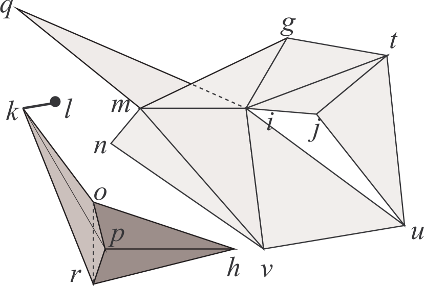
(a)

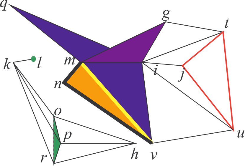
(b)

Figure 3.1: An example of a geometric realization of an abstract simplicial complex (a) and examples (b) of some combinatorial concepts (See § 3.2.2).

Example 3.2.1.

In Figure 3.1a we depict a polyhedron of ${\rm I\kern-1.99997ptR}^{3}$ that is a geometric simplicial complex. In turn this geometric simplicial complex can be seen as the geometric realization of an abstract simplicial complex. Let us call $\Omega$ this abstract simplicial complex. According to the conventions outlined above, we will say, for instance, that the abstract simplicial complex $\Omega$ in Figure 3.1a is a $3$-complex.

In this view, the finite set of points of ${\rm I\kern-1.99997ptR}^{3}$ $\{g,h,i,j,k,\ldots\},$ in Figure 3.1a, stands for the set of Vertices of the abstract simplicial complex $\Omega$. Similarly, in examples, we will talk about points, edges, triangles and tetrahedra to mean the corresponding simplices in the abstract simplicial complex $\Omega$, and so, for instance, the segments $kr$, $kp$, $ko$, $kl$, stands, respectively, for the $1$-simplices $\{k,r\}$, $\{k,p\}$, $\{k,o\}$, $\{k,l\}$ of $\Omega$. Similarly the $mnv$ triangle in the geometric complex in Figure 3.1 stands for the $2$-simplex $\{m,n,v\}$ in the abstract simplicial complex $\Omega$. The presence of two tetrahedra in Figure 3.1a: $kopr$ (in light gray) and $hrop$ (in dark gray) means that in $\Omega$ we have just two $3$-simplices $\{k,o,p,r\}$ and $\{h,r,o,p\}$. Finally note that a simplex is a face of another simplex in $\Omega$ if and only if  this face relation holds in the geometric example. For instance, in Figure 3.1a we have that, in ${\rm I\kern-1.99997ptR}^{3}$, the triangle $rop$ is face of both $kopr$ and $hrop$. At a combinatorial level we will have that the simplex $\{r,o,p\}$ in $\Omega$ is a face for both $\{k,o,p,r\}$ and $\{h,r,o,p\}$.

In the following, we will mainly introduce definitions and properties for abstract simplicial complexes. Therefore, whenever there is no ambiguity, we will freely use the terms simplex and complex to mean abstract simplex and abstract simplicial complex. On the other hand the adjective geometric will be assumed (and therefore omitted) when dealing with geometric examples.

3.2.2 Boundary, Star, Link, Subcomplexes and Closures

The boundary $\partial\gamma$ of a simplex $\gamma$ is defined to be the set of all proper faces of $\gamma$. Similarly, the coboundary or star of a simplex $\gamma$ is defined as $\star{\gamma}=\{\xi\in\Omega\ |\ \gamma\subseteq\xi\}$. Cells $\xi$ in $\star{\gamma}$ are called cofaces of $\gamma$. Any simplex $\gamma$ such that $\star{\gamma}=\{\gamma\}$ is called a top simplex of $\Omega$. Two distinct simplices are said to be incident if and only if  one of them is a face of the other.

The link of a simplex $\gamma$, denoted by $lk(\gamma)$, is the set of all faces of cofaces of $\gamma$, that are not incident to $\gamma$.

The star and the link of a simplex $\gamma$ are defined by referring to the surrounding complex $\Omega$. We can emphasize this reference by using $star({\gamma},{\Omega})$, instead of $\star{\gamma}$ and $lk({\gamma},{\Omega})$, instead of $lk(\gamma)$.

Example 3.2.2.

Considering the complex $\Omega$ in Figure 3.1b we have that the boundary of the triangle $jtu$ is $\partial jtu=\{j,t,u,jt,ju,tu\}$ (in red) and the star (coboundary) of simplex $mi$ is given by $\star{mi}=\{mi,mig,miq,mij\}$ (in violet blue). The link of point $k$ can be found considering the simplices contaning $k$, i.e. $\star{k}=\{k,kl,ko,kp,kr,kop,kpr,kor,kopr\}$ and taking the set of faces not containing the point $k$ , i.e. the triangle $opr$, vertex $l$ together with all triangle faces and hence $lk(k)=\{l,o,p,r,op,pr,ro,opr\}$ (in green). Finally we note that the top simplices in $\Omega$ are eleven: the eight grey triangles on the right of Figure 3.1a and the two tetrahedra $kopr$, $hopr$ and the edge $kl$.

A subset $\Gamma$ of $\Omega$ is closed (in $\Omega$) if, for every simplex $\gamma\in\Gamma$ we have that $\partial\gamma\subset\Gamma$ i.e. all simplices of the boundary of $\gamma$ are also simplices of $\Gamma$. Note that a closed subset of $\Omega$ is always a complex.

A subset of simplices $\Omega^{\prime}\subset\Omega$ is a complex on its own if and only if  $\Omega^{\prime}$ is a closed set of simplices. In this case $\Omega^{\prime}$ is said to be a subcomplex of $\Omega$. In general, given a set of simplices $\Gamma$, the closure $\overline{\Gamma}$ of $\Gamma$ is the smallest subcomplex whose simplices include those in $\Gamma$. In particular, for a simplex $\gamma$, we will use the notation $\overline{\gamma}$ as a shortcut for $\overline{\{\gamma\}}$.

Example 3.2.1.

Consider, for instance, the following three subsets of the abstract simplicial complex $\Omega$ in Figure 3.1b: $A=\{mnv\}$ (in orange); $B=\{mnv,mn,nv\}$ (in black and orange); $C=\{m,n,v,mn,nv,vm,mnv\}$ (in black, orange and yellow). Both subsets $A$ and $B$ are not closed in the original complex $\Omega$, while $C$ is closed in the original complex $\Omega$ and $C=\overline{A}=\overline{B}$.  

Note that the star of a simplex is very rarely a subcomplex while the link of a simplex is always a subcomplex. With these definitions, we can write that, for simplex $\gamma$, $lk(\gamma)=\overline{\star{\gamma}}-\star{\overline{\gamma}}$. Again, we can emphasize the dependence of the link on the complex $\Omega$ by writing the identity $lk(\gamma)=\overline{\star{\gamma}}-\star{\overline{\gamma}}$ as $lk({\gamma},{\Omega})=\overline{star({\gamma},{\Omega})}-star({\overline{\gamma}},{\Omega})$.

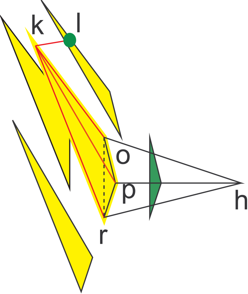
(a)

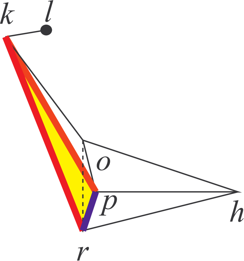
(b)

Figure 3.2: Examples of some combinatorial identities in a $3$-complex (See § 3.2.2).

Example 3.2.3.

In the complex of Figure 3.2a we already noted that $lk(k)=\{l,o,p,r,op,pr,ro,opr\}$ (in green). It is easy to see that $\star{k}=\{k,kl,ko,kp,kr,kop,kpr,kor,kopr\}$ (in yellow, green and red in Figure 3.2a) and $\overline{\star{k}}=\star{k}\cup\{l,o,p,r,op,pr,ro,opr\}$. Therefore $lk(k)=\overline{\star{k}}-\star{k}$ being $k=\overline{k}$. Note again that $\star{k}$ is not a closed subcomplex.

Let us consider Figure 3.2b and the subcomplex $\Delta=\overline{kpr}=\{kpr,kp,kr,pr,k,p,r\}$ ($\Delta$ is in red, blue and yellow in Figure 3.2b). It is easy to see, by definition, that $lk({k},{\Delta})$ is given by the blue segment $rp$ in Figure 3.2b. Let us verify this using the identity $lk({\gamma},{\Omega})=\overline{star({\gamma},{\Omega})}-star({\overline{\gamma}},{\Omega})$ with $\Omega=\Delta$ and $\gamma=\{k\}$. Note that where this is not ambiguous, we use $k$ as a shortcut for $\{k\}$. It is easy to see that $star({k},{\Delta})=\{k,kp,kr,kpr\}$ (in red and yellow) and taking the closure $\overline{star({k},{\Delta})}$ in $\Delta$ we have $\overline{star({k},{\Delta})}=star({k},{\Delta})\cup\{p,r,pr\}$. Therefore, being $k=\overline{k}$, we rewrite the identity $lk({\gamma},{\Delta})=\overline{star({\gamma},{\Delta})}-star({\overline{\gamma}},{\Delta})$ as $lk({k},{\Delta})=\overline{star({k},{\Delta})}-star({k},{\Delta})=\{p,r,pr\}$ and find the blue segment $pr$ plus all its faces. Note that $lk({k},{\Omega})$ is the subcomplex in green in Figure 3.2a and, therefore, $lk({k},{\Delta})\neq lk({k},{\Omega})$

Let $\Phi$ and $\Gamma$ be two set of simplices such that for every $\phi\in\Phi$ and $\gamma\in\Gamma$ we have $\phi\cap\gamma=\emptyset$. We define (following for instance [119] Pg. 109) the join $\Phi\bullet\Gamma$ as the set of simplices $\Phi\cup\Gamma\cup(\cup_{\phi\in\Phi,\gamma\in\Gamma}\{\phi\cup\gamma\})$. We note that the join operator $\bullet$ is both commutative and associative and, for any set of simplices $\Gamma$, we have $\Gamma\bullet\emptyset=\emptyset\bullet\Gamma=\emptyset$.

It is easy to prove that if $\Phi$ and $\Gamma$ are two abstract simplicial complexes, then the join $\Phi\bullet\Gamma$ is an abstract simplicial complex. In particular for a simplex $\gamma$ we write $\gamma\bullet\Phi$ as shorthand for $\overline{\{\gamma\}}\bullet\Phi$. If $\phi$ and $\gamma$ are two disjoint simplices we denote with $\phi\bullet\gamma$ the complex $\phi\bullet\gamma=\overline{\{\phi\}}\bullet\overline{\{\gamma\}}=\overline{\phi\cup\gamma}$. If $\gamma$ is made up of single vertex $w$ we will call the join $\{w\}\bullet\Phi$ the cone from $w$ to $\Phi$.

Where this is not ambiguous we will use the notation $\phi\bullet\gamma$ also to denote the simplex $\phi\cup\gamma$. With this notation we have that the link of $\gamma$ in a certain complex $\Omega$ is given by $lk({\gamma},{\Omega})=\{\phi\in\Omega|\gamma\bullet\phi\subset\Omega\}$ Similarly it is easy to verify that $\overline{\star{\gamma}}=\overline{\gamma}\bullet lk(\gamma)$.

Example 3.2.4.

As an example let us consider an application of join between complexes to compute the closed star of vertex $k$ in Figure 3.2a using formula $\overline{\star{\gamma}}=\overline{\gamma}\bullet lk(\gamma)$. We already know that $\overline{\star{k}}$ is given by all the colored parts in Figure 3.2a. In the complex of Figure 3.2a we have that $lk(k)=\{l,o,p,r,op,pr,ro,opr\}$ (in green in Figure 3.2a). The identity $\overline{\star{\gamma}}=\overline{\gamma}\bullet lk(\gamma)$. with $\gamma=\{k\}$ becomes $\overline{\star{k}}=k\bullet lk(k)$, where we used $k$ as a shortcut for $\{k\}$ and for $\{k\}=\overline{\{k\}}$. To join $k$ with its link we just have to join $k$ with $l$ and $opr$. By definition of join we have that $\{k\}\bullet\{l\}=\overline{kl}$ (i.e. the $kl$ edge). Similarly, joining $k$ with triangle $opr$ we get the tetrahedron $kopr$ (in red, green and yellow in Figure 3.2a). This shows that joining $k$ with its link we obtain the closed star of $k$.

3.2.3 Adjacency, Paths and Connected Complexes

Two simplices are called $s$-adjacent if they share an $s$-face; in particular, two $p$-simplices are said to be adjacent if they are $(p-1)$-adjacent.

A $h$-path is a sequence of simplices $(\gamma_{i})_{i=0}^{k}$ such that two successive simplices $\gamma_{i-1}$ $\gamma_{i}$ are $h$-adjacent. Two simplices $\gamma$ and $\gamma^{\prime}$ are $h$-connected, iff  there exist a $h$-path $(\gamma_{i})_{i=0}^{k}$ such that $\gamma$ is a face of $\gamma_{0}$ and $\gamma^{\prime}$ is a face of $\gamma_{k}$. A subset $\Omega^{\prime}$ of a complex $\Omega$ is called $h$-connected iff every pair of its vertices are $h$-connected. Any maximum $h$-connected subcomplex of a complex $\Omega$ is called a $h$-connected component of $\Omega$. Usually (see [2] Pg. 40) when one forget to mention $h$ and talks about ”connectivity” means $0$-connectivity.

Example 3.2.2.

According to the definition above, the pair of tetrahedra $kopr$ and $hopr$ in the complex of Figure 3.3a are both $0$-adjacent, $1$-adjacent and $2$-adjacent. Hence they also represent a pair of adjacent $3$-simplices. It is easy to show that the complex of Figure 3.3a has two connected components one of which is formed by the three simplices $kl$, $kopr$, and $hopr$ (with all their faces) and the other which is formed by the eight gray triangles on the right. For any pair of simplices in each component there exist a path in between. For instance, the two simplices $l$ and $h$ are connected by the thick gray path $(lk,kr,rh)$. Simplices $gm$ and $nv$ are $0$-connected via the black thick $0$-path $(gm,mn,nv)$. The $2$-simplices $gmi$ and $nvm$ are $1$-connected via the three dark gray triangles that belongs to the $1$-path $(gmi,mvi,nvm)$. With similar remarks one can show that the subcomplex made up of the eight gray triangles is a $1$-connected $2$-complex.  

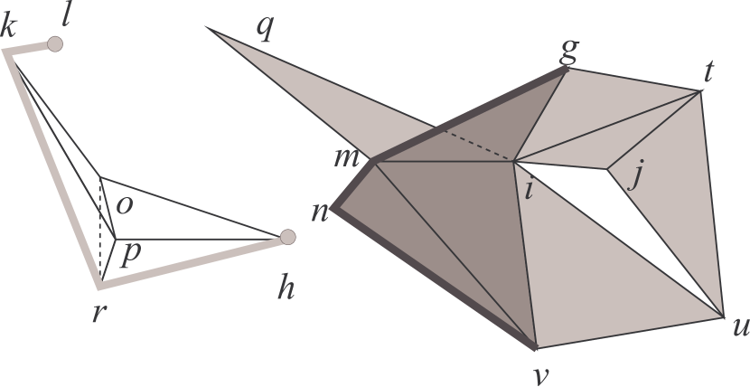
a

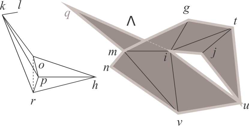
b

Figure 3.3: Examples of paths in connected components (a) (See § 3.2.3) and of regular and non-regular complexes (See § 3.2.4)(b) .

3.2.4 Regular Complexes

A $d$-complex where all top simplices are maximal (i.e. of dimension $d$) is called regular or uniformly $d$-dimensional.

Let $\Omega$ be a regular complex, and $\Omega^{d-1}_{b}$ be the collection of all its $(d-1)$-simplices having only one incident $d$-simplex. The subcomplex $\partial\Omega=\overline{\Omega^{d-1}_{b}}$ is called the boundary of $\Omega$, while the collection of simplices $\Omega-\partial\Omega$ is called the set of internal simplices of $\Omega$.

Example 3.2.3.

The complex of Figure 3.3b is a $3$-complex whose maximal simplices are the two tetrahedra $kopr$ and $hopr$. The complex is not regular since the top simplices are not only the two tetrahedra $kopr$ and $hopr$ but also the edge $kl$ and the the eight gray triangles on the right, The whole complex is not regular while there are three regular subcomplexes that are the closure of $\{kopr,hopr\}$, the edge $kl$ and the complex $\Lambda$ made up of the eight gray triangles on the right. The boundary of $\Lambda$ is given by the eleven thick gray segments in Figure 3.3b.  

3.3 Abstract Simplicial Maps

3.3.1 Introduction

In this paragraph we introduce abstract simplicial maps and show that they provide a categorical structure for abstract simplicial complexes. In this section, we follow mainly the approach in [2, 45, 119] and define (abstract) simplicial maps as applications between (abstract) simplicial complexes. Other approaches [52, 25, 118] define simplicial maps as applications between geometric simplicial complexes. We retain both approaches here in order to state some results in their original form. In order to make a clear distinction between these two options we will call abstract simplicial maps those between abstract simplicial complexes and geometric simplicial maps those between geometric simplicial complexes.

3.3.2 Abstract Simplicial Maps

Let $\mathcal{V}$ be a set of symbols, that we call the universe of vertices. W.l.o.g., from now on we will assume that all complexes have their vertices in $\mathcal{V}$. A vertex map is any map $f$ between vertices, i.e., ${f}:{\mathcal{V}}\rightarrow{\mathcal{V}}$. Moreover, given a vertex map $f$, we will use notation $f[a\mapsto x,b\mapsto y,\ldots]$ as a shorthand for the map $f^{\prime}$ that differs from $f$ only at vertices specified between brackets, i.e., $f^{\prime}(a)=x$, $f^{\prime}(b)=y$, and so on. If $W$ is a set of vertices we will use $[W\mapsto x]$ as a shortcut for $[w\mapsto x|w\in W]$. We will denote by ${\Lambda}:{\mathcal{V}}\rightarrow{\mathcal{V}}$ the identity vertex map and we will use the notation $[a\mapsto x,b\mapsto y,\ldots]$ as a shortcut for $\Lambda[a\mapsto x,b\mapsto y,\ldots]$

Definition 3.3.1 (Abstract Simplicial Map).

Given a pair of abstract simplicial complexes $\Omega$ and $\Omega^{\prime}$ we will say that a vertex map $f$ defines (or induces) a simplex map from $\Omega^{\prime}$ to $\Omega$ if for every simplex $\gamma\in\Omega^{\prime}$ the set of Vertices $f(\gamma)=\{f(v)\ |\ v\in\gamma\}$ is a simplex in $\Omega$. We will use the term abstract simplicial map to denote both vertex maps and simplex maps.

Obviously an abstract simplicial maps preserve the face relation i.e. if $\gamma\leq\beta$ then $f(\gamma)\leq f(\beta)$. We can extend abstract simplicial map from simplices to complexes by defining $f(\Omega^{\prime})=\{f(\gamma)\ |\ \gamma\in\Omega^{\prime}\}$. It is easy to see that if $\Omega^{\prime}$ is a complex, then $\Omega=f(\Omega^{\prime})$ is a complex, too. In the following we will use $f^{-1}(v)$ to denote the inverse image along ${f}:{\mathcal{V}}\rightarrow{\mathcal{V}}$. of the set $\{v\}$. Similarly will use $f^{-1}(\gamma)$ to denote the inverse image along the simplex map induced by $f$ of the set $\{\gamma\}$. Note that, with this notation $f^{-1}(v)$ denotes a set of vertices, while $f^{-1}(\{v\})$ denotes a set of simplices.

In the following we will often use the same symbol (e.g., $f$) to denote both the vertex map and the simplex map . Similarly we will use the same symbol (e.g., $f^{-1}$) to denote the two inverses. However, note that by no means $f^{-1}(\gamma)$ can be recovered using only the knowledge of all sets $f^{-1}(v)$ for all $v\in\gamma$.

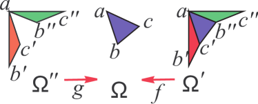
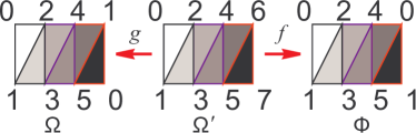
(a) (b)

Figure 3.4: Examples of: two distinct abstract simplicial maps with $f^{-1}(v)=g^{-1}(v)$ for all $v$ (a); two distinct vertex map with the same simplex stitching on top simplices (b)

Example 3.3.1.

Consider for instance the three complexes $\Omega$, $\Omega^{\prime}$ and $\Omega^{\prime\prime}$ in Figure 3.4a. We have that $f(\Omega^{\prime})=\Omega$ and $g(\Omega^{\prime\prime})=\Omega$. For all Vertices $v$ in $\Omega$ we have $f^{-1}(v)=g^{-1}(v)$ and yet the two maps $f$ and $g$ are different. In fact we have $f^{-1}(a)=g^{-1}(a)=\{a\}$; $f^{-1}(b)=g^{-1}(b)=\{b^{\prime},b^{\prime\prime}\}$ and $f^{-1}(c)=g^{-1}(c)=\{c^{\prime},c^{\prime\prime}\}$. Nevertheless $f^{-1}(abc)=\Omega^{\prime}$ and $g^{-1}(abc)=\Omega^{\prime\prime}$.  

Similarly note that the knowledge of the restriction of a simplex map $f$ to top simplices is not sufficient to define $f$ completely.

Example 3.3.2.

In Figure 3.4b we have an example of two abstract simplicial map with the same simplex map on triangles (and on edges) and distinct vertex maps. In fact the vertex maps $f=[6\mapsto 0,7\mapsto 1]$ and $g=[6\mapsto 1,7\mapsto 0]$ induces two simplex stitchings ${f}:{\Omega^{\prime}}\rightarrow{\Phi}$ and ${g}:{\Omega^{\prime}}\rightarrow{\Omega}$ such that, for any $x$, $y$ and $z$ $f(xyz)=g(xyz)$ and $f(xy)=g(xy)$. However, note that $f$ and $g$ are not strictly the same simplex map since their codomain $\Phi$ and $\Omega$ are not isomorphic. This can easily be proven (see also the comment on Figure 3.5a) by noticing that $\Phi$ is orientable while $\Omega$ it is not. Furthermore, obviously, $f$ and $g$ differ on $0$-simplices.  

3.3.3 Isomorphism

A particular class of simplicial maps is given by maps induced by a consistent renaming of Vertices. Such a kind of mapping is called an isomorphism.

Definition 3.3.2 (Isomorphism).

An isomorphism is a bijective abstract simplicial map.

A standard characterization of isomorphic complexes is therefore the following.

Definition 3.3.3 (Isomorphic Complexes (see [74] Pg. 301)).

Two abstract simplicial complexes $\Omega$ and $\Omega^{\prime}$ are isomorphic (written $\Omega\cong\Omega^{\prime}$) if and only if  there exist a bijection between their vertices that induces a bijection between their simplices.

Indeed, it is easy to prove (see [45] Prop. 2.5.2) that a simplicial map induced by a bijection between Vertices is an isomorphism; that the composition of two isomorphisms is an isomorphism and that the inverse map of an isomorphism is an isomorphism, too.

The following property gives another characterization of isomorphic complexes.

Property 3.3.1.

Two abstract simplicial complexes $\Omega$ and $\Omega^{\prime}$ are isomorphic if and only if  there exist two abstract simplicial maps $f$ and $g$ s.t. $f(\Omega^{\prime})=\Omega$ and $g(\Omega)=\Omega^{\prime}$

Proof 3.3.4.

First note that if $\Omega$ and $\Omega^{\prime}$ are isomorphic there exist a bijection $h$ between vertices that is also a bijection between simplices therefore we have an invertible simplicial map whose inverse is again a simplex map therefore taking $f=h$ and $g=h^{-1}$ we prove that for an isomorphic pair of complexes $\Omega$ and $\Omega^{\prime}$ there exist two abstract simplicial maps $f$ and $g$ s.t. $f(\Omega^{\prime})=\Omega$ and $g(\Omega)=\Omega^{\prime}$.

Conversely if such an $f$ and a $g$ exist, then both the vertex map $f$ and the induced simplex map $f$ must be surjective since it spans all vertices and all simplices in $\Omega$. Therefore the number of vertices (simplices) in $\Omega$ is smaller or equal to the number of vertices (simplices) in $\Omega^{\prime}$. Using the same argument for $g$ we conclude that also $g$ must be surjective and hence the number of vertices (simplices) in $\Omega$ must be equal to the number of vertices (simplices) in $\Omega^{\prime}$. Since no vertex can disappear, $f$ must be a bijection between vertices. Since $f$ is an abstract simplicial map the simplex map $f$ must be also a bijection between simplices. Note that not necessarily $f=g^{-1}$.

It is easy to see that the set of abstract simplicial complexes can be equipped with a categorical structure using abstract simplicial maps as morphisms. This provides the set of abstract simplicial complexes with a preorder (see Section A.2 in Appendix A for the definition of preorder)

Property 3.3.2.

The set of abstract simplicial complexes becomes a category using abstract simplicial maps as morphisms. Furthermore, the set of abstract simplicial complexes has a preorder $\prec$. This preorder is completely defined by asking that $\Omega\prec\Omega^{\prime}$ if and only if  there exist an abstract simplicial map $f$ s.t. $f(\Omega^{\prime})=\Omega$.

Proof 3.3.5.

The categorical structure (see, for instance, [119] Pg. 14 and Pg. 110) comes form the fact that the functional composition of two abstract simplicial maps is still an abstract simplicial map. Since $\Lambda(\Omega)=\Omega$ we have that $\Omega\prec\Omega$ (i.e. $\prec$ is reflexive and the identity is a morphism). Transitivity again comes easily from the fact that the composition of two abstract simplicial maps is still an abstract simplicial map.

Note that to have a preorder we just need a a reflexive and transitive relation. In fact, in general $\Omega\prec\Omega^{\prime}$ and $\Omega^{\prime}\prec\Omega$ do not implies $\Omega^{\prime}=\Omega$. However, by Property 3.3.1, this implies that the two abstract simplicial complexes $\Omega$ and $\Omega^{\prime}$ are isomorphic.

Now we can give similar definitions for maps between geometric simplicial complexes. Following this idea we will report the definitions for geometric simplicial maps and geometric simplicial equivalence. Indeed note that a geometric simplicial map is actually a map between a pair of polyhedra $P$ and $P^{\prime}$. Such a map can be a geometric simplicial map or not with reference to a particular pair of geometric simplicial complexes $K$ and $K^{\prime}$. These geometric simplicial complexes $K$ and $K^{\prime}$ must be chosen such that $P=|K|$ and $P^{\prime}=|K^{\prime}|$. This is expressed by the following definition.

Definition * 3.3.5 (Geometric Simplicial Map (See [118] Pg. 520)).

A continuous map ${\phi}:{|K|}\rightarrow{|L|}$ is a geometric simplicial map w.r.t. the geometric simplicial complexes $K$ and $L$ if and only if :

1. for every set of geometric vertices $A=\{{\bf{p}}_{i}\}$ that spans a geometric simplex $\sigma_{A}$ in $K$, the set $\phi(A)$ spans a geometric simplex in $L$.

2. for every geometric vertex ${\bf{p}}\in\sigma_{A}$ if $\lambda_{i}$ are such that ${\bf{p}}=\Sigma_{i}{\lambda_{i}{\bf{p}}_{i}}$ then we have $\phi({\bf{p}})=\Sigma_{i}{\lambda_{i}\phi({\bf{p}}_{i})}$

The second condition in the above definition implies that a geometric simplicial map ${\phi}:{|K|}\rightarrow{|L|}$ is completely determined by its restriction to the set of geometric vertices of $|K|$.

It is easy to show (see [119] Pg. 113) that there is a category of polyhedra and of geometric simplicial maps. There is an obvious equivalence between this category and the category of abstract simplicial complexes and abstract simplicial maps. In fact let $\Omega$ and $\Omega^{\prime}$ be two abstract simplicial complexes with vertices in $V$ and $V^{\prime}$. Let us consider two injective mappings ${{\bf{p}}}:{V}\rightarrow{{\rm I\kern-1.99997ptR}^{n}}$ and ${{\bf{p}}^{\prime}}:{V^{\prime}}\rightarrow{{\rm I\kern-1.99997ptR}^{m}}$ and let $K$ and $K^{\prime}$ be the geometric realization of $\Omega$ and $\Omega^{\prime}$ defined by ${\bf{p}}$ and ${\bf{p}}^{\prime}$. Now, for any abstract simplicial map ${f}:{\Omega^{\prime}}\rightarrow{\Omega}$, there is a geometric simplicial map ${\phi}:{|K^{\prime}|}\rightarrow{|K|}$ given by $\phi({\bf{x}})={\bf{p}}(f({{\bf{p}}^{\prime}}^{-1}({\bf{x}})))$. Conversely, any geometric simplicial map ${\phi}:{|K^{\prime}|}\rightarrow{|K|}$ defines an abstract simplicial map ${f}:{\Omega^{\prime}}\rightarrow{\Omega}$ given by $f(v)={\bf{p}}^{-1}(\phi({{\bf{p}}^{\prime}}(v)))$. With the above naming, the correspondence between $f$ and $\phi$ is expressed by the following commutative diagram.

$$\begin{CD}\Omega @>{f}>{}>\Omega^{\prime}\\ @V{{\bf{p}}}V{}V@V{}V{{\bf{p}}^{\prime}}V\\ |K|@>{\phi}>{}>|K^{\prime}|\end{CD}$$

Note that $f$ and $\phi$ are well defined being ${\bf{p}}^{-1}$ and ${{\bf{p}}^{\prime}}^{-1}$ defined over points (i.e. geometric $0$-simplices) of $K$ and $K^{\prime}$. Very often the geometric simplicial map $\phi$ corresponding to an abstract simplicial map $f$ is denoted by $|f|$. It is easy to show (see [45] Pg. 104) that for any abstract simplicial map $f$ and $g$ we have that $|f|$ is continuos w.r.t. the standard Euclidean topology over ${\rm I\kern-1.99997ptR}^{n}$. Furthermore we have that $|fg|=|f||g|$ and that $f$ is an isomorphism if and only if  $|f|$ is an homeomorphism (see [2] Pg. 48). A more general approach, that do not assume $|K|$ to be imbedded into ${\rm I\kern-1.99997ptR}^{n}$, is possible but is outside the scope of this work (see [119] Pg. 110-114).

The notion of isomorphism is categorical and hence created and preserved when passing from the category of abstract simplicial complex to the equivalent category of geometric simplicial complexes. The created isomorphism induce an isomorphism relation between pairs of geometric simplicial complexes. This is usually called geometric simplicial equivalence. The following definition gives the standard characterization for this equivalence.

Definition * 3.3.5 (Geometric Simplicial Equivalence (See [118] Pg. 520)).

Two geometric simplicial complexes $K$ and $L$ are simplicially equivalent or simplicially isomorphic if and only if  there are two geometric simplicial maps ${\phi}:{|K|}\rightarrow{|L|}$ and ${\psi}:{|L|}\rightarrow{|K|}$ such that $\phi(|K|)=|L|$ and $\psi(|L|)=|K|$. In this case we will write $K\cong L$.

For sake of simplicity, here and in the following, we omit the adjective geometric and talk about simplicial equivalence to mean geometric simplicial equivalence. On the other hand, the term isomorphism will be reserved to the corresponding relation between abstract simplicial complexes.

The equivalence between the category of abstract simplicial complex an the category of geometric simplicial complexes implies that two abstract simplicial complexes are isomorphic if and only if  they have simplicially equivalent geometric realizations. In particular, geometric simplicial complexes that are geometric realizations of a complex $\Omega$ are all simplicially equivalent. Therefore all the polyhedra in $\Delta(\Omega)$ must be homeomorphic.

Given two geometric realizations $K$ and $K^{\prime}$ of two abstract simplicial complexes $\Omega$ and $\Omega^{\prime}$, we have seen that there is a one to one correspondence between abstract simplicial maps, between $\Omega$ and $\Omega^{\prime}$, and geometric simplicial maps w.r.t. $K$ and $K^{\prime}$. We have already stressed that, in examples, we use geometric simplicial complexes (e.g. $K$ and $K^{\prime}$) and perspective drawings of polyhedra in ${\rm I\kern-1.99997ptR}^{3}$ (e.g. $|K|$ and $|K^{\prime}|$) as a handy presentation for the corresponding abstract simplicial complexes ($\Omega$ and $\Omega^{\prime}$). Similarly, in examples, we will use geometric simplicial maps (e.g.${|g|}:{|K^{\prime}|}\rightarrow{|K|}$) as a handy presentation for the associated abstract simplicial maps (i.e. ${g}:{\Omega^{\prime}}\rightarrow{\Omega}$). With this assumption, in examples, we will omit the distinction between $g$ and $|g|$ and talk freely about the abstract simplicial map $g$ with no further reference to the geometric simplicial map $|g|$ actually presented in drawings.

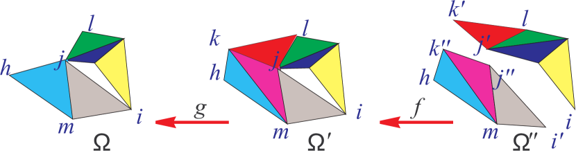
(a)

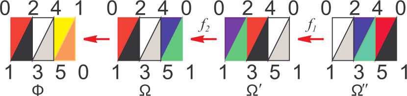
(b)

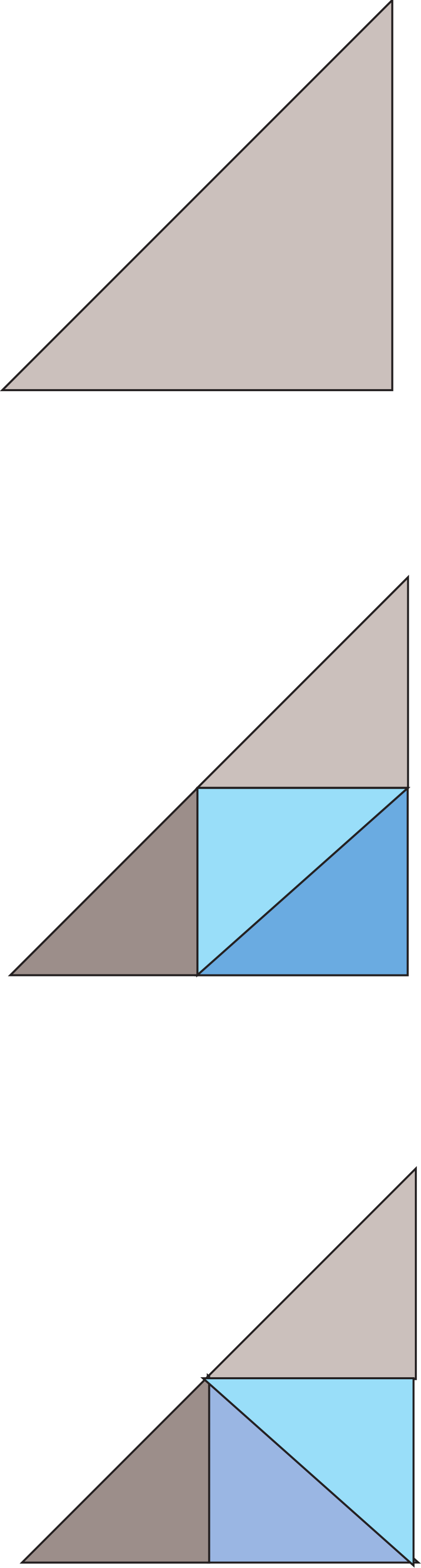
(c)

Figure 3.5: Examples of: abstract simplicial maps (a); two isomorphisms:$f_{1}$ and $f_{2}$ and a complex $\Phi$ non isomorphic with $\Omega$ (b); three complexes that are homeomorphic but not isomorphic (c) (See Example 3.3.6 )

Example 3.3.6.

See now, for example, abstract simplicial maps $f$ and $g$ (represented through geometric simplicial maps) in Figure 3.5a. We have that $f=[k^{\prime}\mapsto k,k^{\prime\prime}\mapsto k,j^{\prime}\mapsto j,j^{\prime\prime}\mapsto j]$, and $g=[k\mapsto j]$. Colors in figures denotes the mapping between triangles i.e., triangles $k^{\prime}j^{\prime}l$ in $\Omega^{\prime\prime}$ and $kjl$ in $\Omega^{\prime}$ receive the same color (red) because $f(k^{\prime}j^{\prime}l)=kjl$. Similarly, there is no red triangle in $\Omega$ because $g$ collapses triangle $kjl$ to edge $jl$ and $kjm$ to edge $jm$. In Figure 3.5b we have three examples of isomorphic complexes $\Omega$, $\Omega^{\prime}$ and $\Omega^{\prime\prime}$. We can see that they are isomorphic by considering the fact that they are linked by two simplicial maps: ${f_{1}}:{\Omega^{\prime\prime}}\rightarrow{\Omega^{\prime}}$ and ${f_{2}}:{\Omega^{\prime}}\rightarrow{\Omega}$ induced by the vertex map $f(x)=x+4\bmod 6$. This vertex map $f$ is a bijection of the set of vertices $\{0,1,2,3,4,5\}$ onto itself. It is easy to check that that $f$ extends to a bijection between simplices. This can be done by checking exhaustively that the six triangles in $\Omega^{\prime\prime}$ (or in $\Omega^{\prime}$) are mapped by $f_{1}$ (or by $f_{2}$) into other six triangles in $\Omega^{\prime}$ (or in $\Omega$). In Figure 3.5b we colored triangles so that a triangle and its the image via $f_{1}$ (or $f_{2}$) receive the same color. For instance triangle $015$ in $\Omega^{\prime\prime}$ and triangle $453$ in $\Omega^{\prime}$ are both in plain black because $f_{1}(015)=453$.

The leftmost complex $\Phi$ is an example of a complex that is not isomorphic to $\Omega$. In fact, any geometric realization of $\Phi$ must be homeomorphic to the Moebius strip and this cannot be homeomorphic to a geometric realizations of $\Omega$. Any geometric realization of $\Omega$ must be homeomorphic to a plain orientable strip i.e., a sphere with two holes. The fact that $\Omega$ and $\Phi$ are not isomorphic can be verified by checking exhaustively that any vertex map associated to a permutation of $\{0,1,2,3,4,5\}$ cannot be extended to a simplex map. If we try, for instance, to extend the identity on $\{0,1,2,3,4,5\}$ from a vertex map to a simplex map we fail because triangle $045$ is not mapped to any triangle (i.e., $045$ does not exist in $\Phi$). Similarly, if we consider vertex map $[2\mapsto 3,3\mapsto 2]$ we have that triangle $345$ is mapped to $245$ that does not exist as a triangle in $\Phi$. An exhaustive analysis of the $6!$ permutations of $\{0,1,2,3,4,5\}$ reveals that the two abstract simplicial complexes $\Phi$ and $\Omega$ are not isomorphic.

However note that, in general, geometric realizations of two non-isomorphic complexes can still be homeomorphic. Let us consider, for instance, the two complexes in Figure 3.5c. They have homeomorphic polyhedra but they are not the same abstract complex. However we can observe that they are related by some sort of subdivision process.

The remark at the end of the previous example is the basis of the definition of a combinatorial analogue of homeomorphism. We will discuss this subject in the next paragraph in order to give a combinatorial definition of manifolds and non-manifolds. The first step in this direction is the definition of stellar equivalence

3.4 Stellar Equivalence

We like to start this section by pointing out that definitions and results outlined in this paragraph account for a theoretical development that started in the 1920’s and 1930’s by M.H. A. Newman [115] and J. W. Alexander [5]. The concept of stellar equivalence brings into the combinatorial framework a concept somehow equivalent to that of homeomorphism. We define stellar equivalence here and discuss the relation between stellar equivalence and homeomorphism. Next, we report limitations on decidability of stellar equivalence. In Section 3.5.2 we will use stellar equivalence to define combinatorial manifolds and non-manifolds.

Definition 3.4.1 (Starring (See [25] Pg. 8)).

Given a $d$-simplex $\gamma\in\Omega$ and a point $w$ s.t. $\{w\}\notin\Omega$ we define the operation of starring the simplex $\gamma$ at the point $w$ as the operation that transforms the complex $\Omega$ into the new complex $\Omega^{\prime}$ obtained from $\Omega$ with the following steps:

• delete the (open) star $\star{\gamma}$;

• for each simplex in $\phi\in\star{\gamma}$ and for each vertex $v\in\gamma$ add the simplex $\{w\}+\phi-\{v\}$ plus all its faces.

In symbols we have that $\Omega^{\prime}=(\Omega-\star{\gamma})\cup(\cup_{\phi\in\star{\gamma},v\in\gamma}\overline{\{w\}+\phi-\{v\}})$

It is easy to prove that the added subcomplex is given by $\{w\}\bullet\partial\gamma\bullet lk(\gamma)$ i.e., $\Omega^{\prime}=(\Omega-\star{\gamma})\cup\{w\}\bullet\partial\gamma\bullet lk(\gamma)$. We will say that $\Omega^{\prime}$ is obtained from $\Omega$ by the elementary stellar subdivision of the simplex $\gamma$ at point $w$ and we will use the notation $\Omega\stackrel{{\scriptstyle(\gamma,w)}}{{\longrightarrow}}\Omega^{\prime}$ to denote this. A stellar subdivision of $\Omega$ is any abstract simplicial complex $\Omega^{\prime}$ obtained by a sequence of elementary stellar subdivisions on $\Omega$.

Similarly when complex $\Omega^{\prime}$ is given and a vertex $w$ in $\Omega^{\prime}$ is such that there exist $\gamma$ and $\Omega$ for which $\Omega\stackrel{{\scriptstyle(\gamma,w)}}{{\longrightarrow}}\Omega^{\prime}$ we will say that we can weld $\Omega^{\prime}$ at $w$ yielding $\gamma$. We will express this with the notation $\Omega^{\prime}\stackrel{{\scriptstyle{(\gamma,w)}^{-1}}}{{\longrightarrow}}\Omega$. We will say that $\Omega$ is obtained from $\Omega^{\prime}$ by the stellar weld at point $w$ yielding the simplex $\gamma$.

The term starring operation will be used to denote both stellar weld and elementary stellar subdivision. Two abstract simplicial complexes $\Omega$ and $\Omega^{\prime}$ will be stellar equivalent (denoted by $\Omega\sim\Omega^{\prime}$) if and only if  there exists a finite sequence of starring operations and simplicial isomorphisms that transforms $\Omega$ into $\Omega^{\prime}$.

A theorem by Neumann [101] proves that restricting starring operations to 1-simplices we still obtain the stellar equivalence defined above.

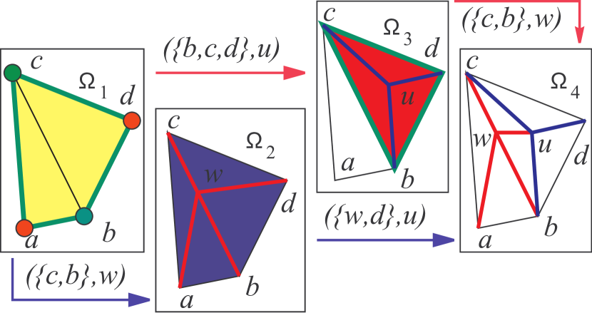
a

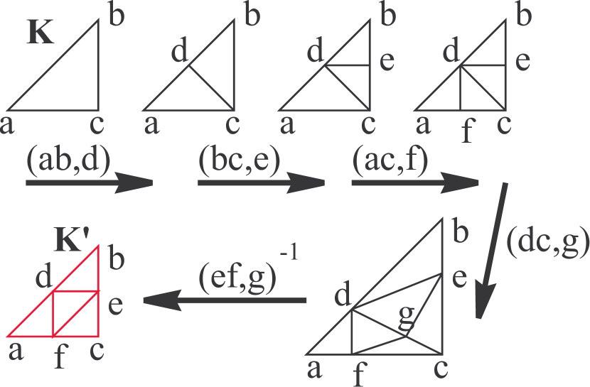
b

Figure 3.6: Starring (a) and stellar equivalence (b) (See Example 3.4.2 for (a) and 3.4.1 for (b) )

Example 3.4.2.

As an example of application of this definition consider, for instance, the abstract simplicial complex $\Omega_{1}$ in Figure 3.6a. Complexes $\Omega_{2}$ and $\Omega_{3}$ are stellar subdivisions of complex $\Omega_{1}$ obtained by stellar subdivision of, respectively, edge $\{b,c\}$ at $w$ and of triangle $\{b,c,d\}$ at $u$ i.e., in symbols, $\Omega_{1}\stackrel{{\scriptstyle(\{b,c\},w)}}{{\longrightarrow}}\Omega_{2}$ and $\Omega_{1}\stackrel{{\scriptstyle(\{b,c,d\},u)}}{{\longrightarrow}}\Omega_{3}$.

Let us consider in detail the first stellar subdivision along the blue path i.e., $\Omega_{1}\stackrel{{\scriptstyle(\{b,c\},w)}}{{\longrightarrow}}\Omega_{2}$. To subdivide simplex $\{b,c\}$ at $w$ we first delete the yellow triangles $\{a,b,c\}$, $\{b,c,d\}$ and edge $\{b,c\}$ that are the (open) star $\star{bc}$. We leave in place the boundary of this star $\partial(\star{bc})=\overline{\{ca,ab,bd,dc\}}$ (i.e. the thick green lines). Then, according to definition we must add $\{w\}\bullet\partial\{b,c\}\bullet lk(\{b,c\})$. Since $\partial\{b,c\}=\{\{b\},\{c\}\}$ (in green in Figure 3.6a) and $lk(\{b,c\})=\{\{a\},\{d\}\}$ (in red in Figure 3.6a) we add $\{w\}\bullet\{\{b\},\{c\}\}\bullet\{\{a\},\{d\}\}$. The join $\{\{b\},\{c\}\}\bullet\{\{a\},\{d\}\}$ is given by the four segments: $ca$,$ab$,$bd$,$dc$ and therefore we must add the cones from $w$ to these four segment. This gives the four blue triangles in $\Omega_{2}$. We must add these four triangles together with their faces. By taking faces of the blue triangles we also add segments $ca$, $ab$, $bd$ and $dc$. Note that these segments were not deleted since they are not in the open star of $bc$.

Now let us consider in detail the first stellar subdivision along the red path $\Omega_{1}\stackrel{{\scriptstyle(\{b,c,d\},u)}}{{\longrightarrow}}\Omega_{3}$. The starring subdivision of $\{b,c,d\}$ at $u$ is obtained by deleting $\{b,c,d\}=\star{\{b,c,d\}}$. We leave in place the boundary of this star $\partial(\star{bcd})=\overline{\{cb,bd,dc\}}$ (i.e. the thick green lines). After this deletion we add the cone from $u$ to the boundary of triangle $\{b,c,d\}$, being $lk(\{b,c,d\})=\emptyset$. Since $\partial\{b,c,d\}$ is given by the three segments $bc$, $cd$ and $db$ the simplices to be added are obtained by taking the cone from $u$ to these three segments. In this way we obtain the three red triangles of $\Omega_{3}$ in Figure 3.6a. These triangles are added together with their faces. However note that segments $bd$, $dc$ and $cb$, that must be added now, were not deleted removing the open star of triangle $\{b,c,d\}$.

Let us see a very simple example of a stellar equivalence. We want to show that $\Omega_{2}$ and $\Omega_{3}$ are stellar equivalent (i.e. . $\Omega_{2}\sim\Omega_{3}$). We follow blue and red path to $\Omega_{4}$. The blue path is completed by the stellar subdivision of edge $\{w,d\}$ at $u$ in $\Omega_{2}$. The red path is completed by the stellar subdivision of edge $\{b,c\}$ at $w$ in $\Omega_{3}$. Both paths join at $\Omega_{4}$. In symbols we have that: $\Omega_{2}\stackrel{{\scriptstyle(\{w,d\},u)}}{{\longrightarrow}}\Omega_{4}$ and $\Omega_{3}\stackrel{{\scriptstyle(\{b,c\},w)}}{{\longrightarrow}}\Omega_{4}$. The way in which we obtained complex $\Omega_{4}$ proves that complexes $\Omega_{2}$ and $\Omega_{3}$ are stellar equivalent.

Note that if, by any chance, we perform these two last stellar subdivisions by introducing two new Vertices $u^{\prime}$ and $w^{\prime}$, instead of $u$ and $w$ (i.e. if we perform the stellar subdivisions given by $\Omega_{2}\stackrel{{\scriptstyle(\{w,d\},u^{\prime})}}{{\longrightarrow}}\Omega_{4}^{\prime}$ and $\Omega_{3}\stackrel{{\scriptstyle(\{b,c\},w^{\prime})}}{{\longrightarrow}}\Omega_{4}^{\prime\prime}$), we still obtain stellar equivalence between $\Omega_{2}$ and $\Omega_{3}$ since the resulting complexes $\Omega_{4}^{\prime}$ and $\Omega_{4}^{\prime\prime}$, although distinct, are isomorphic. In fact the renaming of Vertices $[u^{\prime}\mapsto u]$ and $[w^{\prime}\mapsto w]$ defines two isomorphisms that sends, respectively ${\Omega_{4}^{\prime}}$ and ${\Omega_{4}^{\prime\prime}}$ into $\Omega_{4}$.

Next we recall here some basic results on stellar equivalence for future reference. A first property of stellar equivalence is that joining stellar equivalent complexes we obtain stellar equivalent complexes.

Property 3.4.1 (See [74] Pg. 303).

Let us consider two pairs, $\Omega_{1}$, $\Omega_{1}^{\prime}$ and $\Omega_{2}$, $\Omega_{2}^{\prime}$, of abstract simplicial complexes such that $\Omega_{1}\sim\Omega_{1}^{\prime}$ and $\Omega_{2}\sim\Omega_{2}^{\prime}$ and such that $\Omega_{1}\bullet\Omega_{2}$ and $\Omega_{1}^{\prime}\bullet\Omega_{2}^{\prime}$ are well defined complexes, then we have $\Omega_{1}\bullet\Omega_{2}\sim\Omega_{1}^{\prime}\bullet\Omega_{2}^{\prime}$

In particular the cone from a vertex to two stellar equivalent complexes gives stellar equivalent complexes.

The next step in this overview will be the presentation of an equivalence between geometric simplicial complexes that mimics stellar equivalence between abstract simplicial complexes. Such an equivalence, called piece-wise linear equivalence, will be used in Section 3.5 to give the (classical) definition of combinatorial manifolds. To develop this notion we first need to introduce the notion of subdivision relation between geometric simplicial complexes.

Definition * 3.4.2 (Subdivision ([52] Pg. 7)).

A geometric simplicial complex $K^{\prime}$ is a subdivision of another geometric simplicial complex $K$ if and only if  $|K|=|K^{\prime}|$ and for every simplex $\sigma^{\prime}\in K^{\prime}$ there exist a simplex $\sigma\in K$ such that $\sigma^{\prime}\subset\sigma$.

Note that, in the condition $\sigma^{\prime}\subset\sigma$, the two simplices $\sigma$ and $\sigma^{\prime}$ are geometric simplices, i.e. subsets of ${\rm I\kern-1.99997ptR}^{n}$.

Example 3.4.1.

It is easy to show that if $\Omega^{\prime}$ is a stellar subdivision of $\Omega$ then there exist two geometric simplicial complexes $K$ and $K^{\prime}$ that are geometric realization of, respectively, $\Omega$ and $\Omega^{\prime}$ such that $K^{\prime}$ is a subdivision of $K$. The converse is not always true. In fact not all subdivisions are stellar subdivisions. This is easy to see considering the two geometric complexes $K$ and $K^{\prime}$ of Figure 3.6b. The geometric complex $K^{\prime}$ (in red) is a subdivision of the complex $K$ (i.e. the single triangle $abc$). The geometric complex $K^{\prime}$ can not be the geometric realization of a stellar subdivision of $abc$. We can prove this by contradiction. Let assume that such a stellar subdivision exist. First we note that every stellar subdivision introduce a new vertex. Therefore just three elementary stellar subdivision must produce the red complex $K^{\prime}$ out of $abc$ introducing $d$, $e$ and $f$. If we consider all the possible moves it is easy to see that every elementary stellar subdivision that introduces a vertex on a boundary edge creates a vertex of order $3$. See for instance the moves in Figure 3.6b. Therefore, the last elementary subdivision of this possible stellar subdivision from $K$ to $K^{\prime}$ must introduce a vertex of order $3$. The contradiction comes from the fact that all added Vertices, i.e. $d$, $e$ and $f$ are of order $4$. Therefore $K^{\prime}$ is not a stellar subdivision of $K$.  

The notion of subdivision seems to be more general than the notion of stellar subdivision. However stellar subdivision admits a combinatorial definition while generic subdivisions do not. Indeed, we can define stellar subdivisions for an abstract simplcial complex $\Omega$ with no reference to its geometric (polyhedral) realization. Stellar subdivisions are not the only possible option for a combinatorial notion of subdivision. Another purely combinatorial definition of a subdivision is the so called barycentric subdivision. Barycentric subdivisions can be defined directly on the abstract simplicial complex with no reference to a geometric realization. We do not report this notion here (see [52] Pg, 7) simply because it can be proved that any barycentric subdivision is a stellar subdivision while the converse it is trivially false. In general the problem of whether stellar subdivision can mimics completely generic subdivisions can be presented as the claim:

Conjecture * 3.4.2.

Let $\Omega$ and $\Omega^{\prime}$ be two abstract simplicial complexes and let $K$ and $K^{\prime}$ be two particular geometric realization for $\Omega$ and $\Omega^{\prime}$, respectively. If $|K|=|K^{\prime}|$ then there exist a common stellar subdivision for $\Omega$ and $\Omega^{\prime}$

The above claim is a classic conjecture (see [25] Pg. 14) that is still unsolved. A purely combinatorial formulation of (a slighty more general version of) the above claim, presented in [74] (see [74] Pg. 311), is the following:

Conjecture * 3.4.3.

Let $\Omega$ and $\Omega^{\prime}$ be two abstract simplicial complexes If $\Omega$ and $\Omega^{\prime}$ are stellar equivalent then there exist a common (up to isomorphism) stellar subdivision for $\Omega$ and $\Omega^{\prime}$.

Since the real power of stellar subdivisions is still an open problem, in the following, we must consider the full stellar equivalence i.e. the equivalence generated by both subdivisions and welds. Stellar equivalence is surely more powerful than equivalence based on stellar subdivisions. In the following, we first give an example of stellar equivalence and then consider the relation between stellar equivalence and another equivalence based on subdivisons (called piecewise linear equivalence).

Example 3.4.2.

The sequence of starring operations in Figure 3.6b shows that $K^{\prime}$ can be the geometric realization of a complex that is stellar equivalent to $K$. This equivalence is established by four subdivisions and a final weld.  

Indeed, as we will see in the following, stellar equivalence and equivalence based on subdivisions are actually the same equivalence. In order to see this, we must carefully define equivalence based on subdivisions. This will bring in the ideas of piecewise linear map and piecewise linear equivalence. These notions will guide us to the definition of an equivalence that is the best combinatorial analogue of homeomorphism for polyhedra.

Definition * 3.4.2 (Piecewise Linear Simplicial Map (See [52] Pg. 13)).

A continuous map ${\phi}:{|K|}\rightarrow{|L|}$ is a piecewise linear (p.l.) simplicial map from the geometric simplicial complex $K$ to the geometric simplicial complex $L$ if and only if  $K$ and $L$ have two subdivisions $K^{\prime}$, $L^{\prime}$ such that $\phi$ is a geometric simplicial map from $K^{\prime}$ to $L^{\prime}$.

In the situation of the above definition, if $K^{\prime}$ and $L^{\prime}$ are simplicially equivalent, then the p.l. simplicial map $\phi$ is a homeomorphism called a piecewise linear homeomorphism. Directly from the definition, it is easy to see that all simplicial maps are p.l. maps and all simplicial homeomorphisms are p.l. homeomorphisms. Geometric simplicial complexes with p.l. simplicial maps constitutes a category (see [52] Theorem I.6). In particular, in this category, we can define an equivalence between geometric simplicial complexes. This will result in the notion of PL-equivalence.

Definition * 3.4.2 (Piecewise Linear Equivalence (PL-equivalence [52] Pg.13)).

Two geometric simplicial complexes $K$ and $L$ are PL-equivalent if and only if  they have two simplicially equivalent subdivisions. In this case we will write $K\approx L$.

Directly from the definition above, we have that two geometric simplicial complexes that are simplicially equivalent must be PL-equivalent. Therefore, all geometric simplicial complexes in $\Delta(\Omega)$ are PL-equivalent. We will say that two abstract simplicial complexes are PL-equivalent if and only if  their carriers contains PL-equivalent polyhedra.

Therefore, we have that PL-equivalence induce an equivalence upon abstract simplicial complexes. This equivalence, although defined using (geometric) subdivisions, must admit a combinatorial definition. This definition is actually given by the notion of stellar equivalence. This is stated by the following theorem that is a central result in combinatorial topology.

Theorem 3.4.3 (Equivalence of Stellar and PL-theory (See [52] Pg. 41 or [74] Pg. 311)).

Let $\Omega$ amd $\Omega^{\prime}$ be two abstract simplicial complexes with geometric realization $K$ and $K^{\prime}$. We have that $\Omega\sim\Omega^{\prime}$ if and only if  $K\approx K^{\prime}$.

On the ground of the previous result, in the following, we will use the term combinatorial equivalence to denote both PL-equivalence and stellar equivalence. Combinatorial equivalence implies homeomorphism between polyhedra that are geometric realizations of combinatorially equivalent complexes. Therefore we have that if $\Omega\sim\Omega^{\prime}$ then $\Delta(\Omega)$ and $\Delta(\Omega^{\prime})$ must contain homeomorphic polyhedra. The converse is the well known Hauptvermutung, which states that two abstract simplicial complexes that have homeomorphic geometric realization are combinatorially equivalent. This property is known to be true for $d$-complexes for $d\leq 2$ [104] and for $d=3$ [94] and it is known to be false in general. In fact, Milnor [93] provided the first example of a pair of non-manifold $7$-complexes that have homeomorphic geometric realizations, and yet are not combinatorially equivalent.

Combinatorial equivalence is not equivalent to homeomorphism for $d$-complexes for $d\geq 7$. However, already for $d\geq 4$, combinatorial equivalence is only semi-decidable. This is a consequence of a result by Markov [88]. This result states that there exist a $4$-complex $\Omega_{0}$ such that it is impossible to decide, for any other complex $\Omega$, if $\Omega_{0}\sim\Omega$.

We end this section by quoting a result that we report for forthcoming reference.

Property 3.4.4.

Let $\Omega$ and $\Omega^{\prime}$ be two stellar equivalent abstract simplicial complexes (i.e. $\Omega\sim\Omega^{\prime}$). Let $w$ be a vertex that remains unchanged across the starring operations that bring $\Omega$ to $\Omega^{\prime}$, then the links $lk({w},{\Omega})$ and $lk({w},{\Omega^{\prime}})$ are stellar equivalent.

Proof 3.4.4.

See Corollary 1.15 in [25] Pg. 23 and Theorem 3.4.3.

3.5 Manifoldness

Having defined combinatorial equivalence, we can step into the definition of combinatorial manifolds. Before doing that, we define a superclass of manifolds called pseudomanifolds and introduce the first notion of non-manifoldness. Next we will introduce topological and combinatorial manifolds and discuss their relation between them.

3.5.1 Pseudomanifolds

Let $\gamma$ be a $(d-1)$-simplex in a $d$-complex $\Omega$. We say that $\gamma$ is a manifold $(d-1)$-simplex if and only if  the closed star of $\gamma$ is a regular $d$-complex containing just one or at most two $d$-simplices incident at $\gamma$.

The two $d$-simplices $\gamma$ and $\gamma^{\prime}$ are said to be manifold connected, in a abstract simplicial complex $\Omega$, if and only if  there exist a sequence of $d$-simplices (called a manifold path) $(\gamma_{i})_{i=0}^{k}$ with $\gamma=\gamma_{0}$, $\gamma^{\prime}=\gamma^{k}$ and such that two successive complexes $\gamma_{i-1}$, $\gamma_{i}$, $i=1,\ldots,k$ are adjiacent via a manifold $(d-1)$-simplex (i.e. $\gamma_{i-1}\cap\gamma_{i}$ is a manifold $(d-1)$-simplex in $\Omega$). Note that we do not ask $\Omega$ to be regular. Proceeding as with $h$-connectivity we can define manifold-connectivity and manifold-connected components.

Having defined manifold $(d-1)$-simplices we can step into the definition of pseudomanifolds.

Definition 3.5.1 (Pseudomanifold see [119] Pg. 150).

A regular $(d-1)$-connected $d$-complex where all $(d-1)$-simplices are manifold is called a combinatorial pseudomanifold (possibly with boundary).

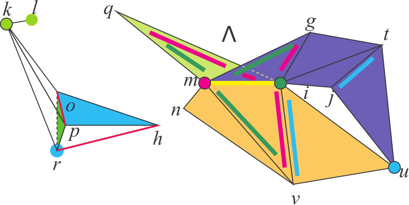
(a)

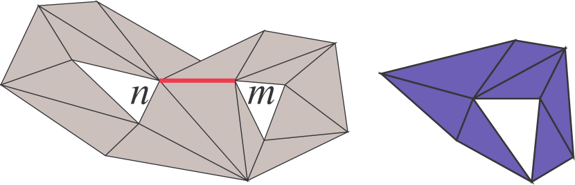
(b)

Figure 3.7: Manifold and non-manifold simplices in a $2$-complex (See Examples 3.5.1) and 3.5.5) .

Example 3.5.1.

Consider, for instance, the subcomplex $\Lambda$ in Figure 3.7a. All $1$-simplices (segments) in the regular $2$-complex $\Lambda$ are manifold $1$-simplices but the segment $mi$ in yellow. This is not a manifold $1$-simplex. The complex $\Lambda$ is neither a pseudomanifold nor a manifold-connected component. It is easy to see that in $\Lambda$ we have three manifold connected components these are respectively the triangle $qmi$, the three orange triangles (i.e. $nmv$,$miv$ and $viu$) and the four violet triangles (i.e. $mig$, $git$, $itj$ and $tju$).

The gray subcomplex in Figure 3.7b is an example of a manifold connected complex that is not a pseudomanifold since the red segment $nm$ is not a manifold $1$-simplex. Finally the blue complex in Figure 3.7b is an example of a $2$-pseudomanifold.  

3.5.2 Topological and Combinatorial Manifolds

In this paragraph we will introduce both topological manifolds and combinatorial manifolds and discuss the distinction between these two definitions.

The definition of combinatorial manifolds, being based on stellar equivalence, is a truly combinatorial definition. By a truly combinatorial definition we mean a definition such that there exist a semi-decision algorithm that stops when it has realized that the input encodes a combinatorial manifold.

We note that combinatorial manifolds are the only known analogue of topological manifolds that admit a semi-decidable definition. This fact, although foundational for geometric modeling and computer graphics, receives little attention in handbooks of combinatorial topology (with the notable exception of [52]). This sort of forgetfulness is clearly pointed out in the survey in [74] that has been a precious help for writing this short introduction to this subject.

Note that combinatorial manifoldness is just semi-decidable and is not decidable. In fact there is no decision procedure that stops and says if the input was a combinatorial $d$-manifold or not. Such an algorithm is impossible to build for $d\geq 6$. This is an easy consequence of a result by S.Novikov [125].

In the standard Euclidean topological space ${\rm I\kern-1.99997ptR}^{d}$ we define the standard closed unit $d$-ball as the set ${\mathcal{B}}^{d}=\{{\bf{x}}\in{\rm I\kern-1.99997ptR}^{d}|\|{\bf{x}}\|\leq 1\}$ where $\|{\bf{x}}\|$ is the standard Euclidean metric over the Cartesian product ${\rm I\kern-1.99997ptR}^{d}$. The standard closed unit $d$-ball in ${\rm I\kern-1.99997ptR}^{d}$ will be denoted by ${\mathcal{B}}^{d}$.

With this definition we can introduce topological manifolds:

Definition * 3.5.1 (Topological $d$-manifold [52]).

A topological connected $d$-manifold is a topological connected metric space where each point has a neighborhood homeomorphic to ${\rm I\kern-1.99997ptR}^{d}$ or to the closed unit ball ${\mathcal{B}}^{d}$ in ${\rm I\kern-1.99997ptR}^{d}$.

An alternative equivalent definition is the following:

Definition * 3.5.1 (Topological $d$-manifold [118] Pag. 518).

A topological connected $d$-manifold is a topological connected metric space where each point has a neighborhood homeomorphic to the standard open unit $d$-ball $\stackrel{{\scriptstyle\circ}}{{{\mathcal{B}}^{d}}}$ or to the closed unit half $d$-ball ${\mathcal{B}}^{d}_{+}$.

We denote with $\stackrel{{\scriptstyle\circ}}{{{\mathcal{B}}^{d}}}$ the standard open unit $d$-ball i.e. the set $\stackrel{{\scriptstyle\circ}}{{{\mathcal{B}}^{d}}}=\{{\bf{x}}\in{\rm I\kern-1.99997ptR}^{d}|\,\|{\bf{x}}\|<1\}$ Similarly we denote with ${\mathcal{B}}^{d}_{+}$ the standard closed unit half $d$-ball i.e. the set ${\mathcal{B}}^{d}_{+}=\{{\bf{x}}\in{\rm I\kern-1.99997ptR}^{d}|\,\|{\bf{x}}\|<1\,\,\mbox{\rm and}\,\,x_{i}\geq 0\,\,\mbox{for}\,\,i=1,\ldots,d\}$

A topological $d$-manifold that is a geometric polyhedron is usually called a triangulable manifold. From this definition, we have that a topological $d$-manifold is triangulable if and only if  it is the carrier of some abstract simplicial complex. Note that there are examples [4] of topological $4$-manifolds that are not triangulable. It is unknown if there exist non triangulable topological $d$-manifolds for $d>4$.

In the following we will use the term standard $d$-simplex to denote the abstract simplicial complex $\Delta^{d}$ obtained as the set of parts of a set of $d+1$ vertices. It is easy to see that the complex $\Delta^{d}$ is defined up to isomorphism.

A combinatorial $d$-ball is any abstract simplicial complex $B^{d}$ that is combinatorially equivalent to $\Delta^{d}$. A combinatorial $d$-sphere is any simplicial complex $S^{d}$ that is combinatorially equivalent to $\partial\Delta^{d+1}$. Note that a combinatorial $0$-ball is any singleton $\{\{v\}\}$ for any vertex $v$, while a combinatorial $0$-sphere, being combinatorially equivalent to $\partial\Delta^{1}$ is any couple $\{\{v\},\{w\}\}$ for any pair of distinct vertices $v$ and $w$.

Definition 3.5.2 (Combinatorial Manifold (see [52] Pg. 19 )).

Let $v$ be a vertex in a regular $d$-complex $\Omega$. We say that $v$ is a manifold vertex if and only if  its link $lk(v)$ is a $(d-1)$-complex that is combinatorially equivalent either to:

1. the boundary of a $d$-dimensional simplex (i.e., a $(d-1)$-sphere) if $v$ is an internal vertex, or to

2. a $(d-1)$-simplex (i.e., a $(d-1)$-ball) if $v$ is a boundary vertex.

Otherwise, we say that $v$ is a non-manifold vertex in $\Omega$.

A regular $d$-complex where all vertices are manifold is called a combinatorial $d$-manifold (possibly with boundary).

It is easy to prove that a combinatorial $d$-manifold is also a combinatorial $d$-pseudomanifold. All combinatorial $d$-manifolds are topological $d$-manifolds. More precisely, it is easy to see that the polyhedron associated to a geometric realization of a combinatorial $d$-manifold is a topological $d$-manifold (Remark Pg. 26 in [25]). Therefore, all polyhedra in the carrier of a combinatorial $d$-manifold are topological manifolds.

However there are topological manifolds that are not contained in the carrier of a combinatorial manifold. In fact, not all topological $d$-manifolds are triangulable as a combinatorial manifold. It has been proved that all topological $1$-manifolds and $2$-manifolds are triangulable as a combinatorial manifold [13]. Also $3$-manifolds are known to be triangulable as combinatorial $3$-manifolds [94]. Freedman (see [48] [49]) constructed an example of a topological $4$-manifold that cannot be triangulated as a combinatorial manifold.

We have seen in Section 3.4 that combinatorial equivalence is less powerful than topological equivalence (i.e. homeomorphism). We recall that Milnor in [93] disproved the Hauptvermutung, by providing the first counterexample in this sense. Milnor counterexample is based on the construction of a pair of $7$-complexes that have homeomorphic geometric realizations and yet that are not combinatorially equivalent. Since these two complexes were non-manifold it is reasonable to ask if the Hauptvermutung can still hold within the class of combinatorial manifolds. This claim was called the manifold Hauptvermutung.

The manifold Hauptvermutung was solved negatively in the late 1960’s [107] [68]. In fact, for instance from the construction in [26], for any $d\geq 5$, one can build an abstract simplicial $d$-complex that is not a combinatorial $d$-manifold and whose carrier is homeomorphic to the standard $d$-sphere. Since the standard $d$-sphere can always be triangulated as a combinatorial $d$-manifold this provides a counterexample to the combinatorial Hauptvermutung, already for $d>5$, in the tiny realm of the triangulations of the $d$-sphere.

Hence, topological manifolds are a proper super-class of combinatorial manifolds and homeomorphism is stronger than combinatorial equivalence even within the subclass of combinatorial manifolds. Furthermore, combinatorial equivalence is just semi-decidable and not decidable even within the subclass of combinatorial manifolds. In fact, the recalled result by Markov [88], already in its original form, applies to $4$-manifolds. We recall that Markov result states that there exist a combinatorial $4$-manifold $\Omega_{0}$ such that it is impossible to decide, for any other combinatorial manifold $\Omega$, if $\Omega_{0}\sim\Omega$.

Another deep theoretical result, by S. Novikov [125], shows that the problem of recognizing the $d$-sphere for $d\geq 5$ implies the problem of recognizing a trivial group in a finite sequence of finitely generated groups. It is known [1] that this problem, in turn, implies the Halting Problem (see [100] Pg. 1-4 for an introduction on the relation between these problems). In [100] the relation between the recognizability of the $d$-sphere and the halting problem is explicitly stated. Thus we report here this latter”effective” version of the Novikov result:

Theorem 3.5.3 (Theorem 2.1 in [100]).

There exist an algorithm which, for any $d\geq 5$, any combinatorial manifold $M$ of dimension $d$, any given Turing machine $T$ and its input $w$ constructs another combinatorial manifold $R_{T}(w)$ such that $M$ and $R_{T}(v)$ are combinatorially equivalent to if and only if  T halts on $w$.

Proof 3.5.4.

Theorem 3.5.3 is essentially an excerpt from Theorem 2.1 in [100]. restated using the the notations in this work.

If we take $M=S^{d}$ and assume that we can recognize the $d$-sphere then, by Theorem 3.5.3, we can decide the Halting Problem.

It is well known [100] that the existence of an algorithm recognizing whether or not a $(d+1)$-complex is a combinatorial $(d+1)$-manifold is equivalent to the recognizability of the $d$-sphere. So, this decision problem is known to be solvable for $d=1,2,3$ [123], unsolvable for $d\geq 5$ and open for $d=4$.

Example 3.5.5.

As an example of application of the above definitions consider, for instance, the complex of Figure 3.7a. According to our definition, Vertices $u$, $m$ and $i$ are non-manifold Vertices. In fact, they are all boundary Vertices and none of the links $lk(u)$ (segments in pale blue), $lk(m)$ (three segments in violet), and $lk(i)$ (three segments in green) is combinatorially equivalent to a $1$-simplex. This can be easily proven by observing that combinatorially equivalent complexes must have homeomorphic geometric realizations and neither the violet, nor the green nor, the pale blue $1$-complexes are homeomorphic to a segment. In fact, the pale blue link is disconnected while, in the violet link, the vertex $i$ is incident to three $1$-simplices. The same problem exists at vertex $m$ in the green link.

In the following we will restrict our attention to combinatorial manifolds. Therefore, in the following, very often, we will omit the term combinatorial and talk about manifolds and manifoldness to mean combinatorial manifoldness.

3.5.3 Non-manifold simplices

We have already defined non-manifold $(d-1)$-simplices and non-manifold vertices in a regular complex. We now extend this definition to any $s$-simplices for any $0\leq s<d$ in an arbitrary (possibly non regular) $d$-complex.

Definition 3.5.6.

Let $\gamma$ be a $s$-simplex in a $d$-complex $\Omega$ with $0\leq s\leq(d-1)$ we will say that $\gamma$ is a manifold $s$-simplex if and only if  $lk(\gamma)$ is a regular $h$-complex that is combinatorially equivalent either to the $h$-sphere or to a $h$-ball, for some $h\leq d-s-1$

Note that the above definition do not require $\Omega$ to be a regular complex. Indeed, if $\Omega$ is a regular $d$-complex we have $h=d-s-1$. In this case, in a regular $d$-complex, for $s=0$ and $s=d-1$ the above definition gives, respectively, the conditions for manifold vertices and manifold $(d-1)$-faces in a regular complex.

An $s$-simplex that is not a manifold $s$-simplex will be called a non-manifold $s$-simplex. In the following, we will see that in a combinatorial manifold all simplices are manifold and hence its boundary is manifold, too. On the other hand we have that a regular complex has non manifold simplices if and only if  it is not a manifold complex. Furthermore we will see that manifoldness is preserved by combinatorial equivalence. A simplex can be manifold even if all its faces are non manifold, while the converse it is not true. This is stated by the following properties.

Property 3.5.1.

1. If $\Omega$ is a combinatorial $d$-manifold then $\partial\Omega$ is a combinatorial $(d-1)$-manifold without boundary.

2. If a combinatorial $d$-manifold $\Omega$ is combinatorially equivalent to another complex $\Omega^{\prime}$, then $\Omega^{\prime}$ is a combinatorial $d$-manifold, too.

3. In a combinatorial manifold all simplices are manifold simplices.

4. All faces of a non-manifold simplex are non manifold simplices.

Proof 3.5.7.

Property 1 is proven in [52] Pg. 21. Properties 2 and 3 are proven in [74] (see Lemma 3.2 p. 304). The property 4 can be proven as follows. Let us assume that there exist a manifold face of a non manifold simplex $\gamma$ and derive a contradiction. Figure 3.8a depicts a situation coherent with the assumption that $\gamma$ (in violet blue) is a non manifold simplex. Let $\zeta$ (vertex in orange) be a manifold face of the non manifold simplex $\gamma$ and let $\omega$ (vertex in green) be such that $\omega\cap\zeta=\emptyset$ and $\gamma=\zeta\cup\omega$, then we have that $\overline{\{\gamma\}}=\zeta\bullet\omega$. Now, it is easy to prove, (see for instance Lemma in [52] Pg. 20) that $lk(\gamma)=lk({\omega},{lk({\zeta},{\Omega})})$ (${lk({\zeta},{\Omega})}$ are the three edges in orange and $lk(\gamma)$ are the three vertices in violet). Since, by hypothesis, $\zeta$ is a manifold simplex, we have that $lk({\zeta},{\Omega})$ (the three thick orange segments) is combinatorially equivalent either to a ball or a sphere and hence, by Part 2 in this property, $lk({\zeta},{\Omega})$ is a manifold complex. Now $\omega$ is a simplex in $lk({\zeta},{\Omega})$ and hence, in this complex, the link of $\omega$ (the three violet blue thick dots), i.e. $lk({\omega},{lk(\zeta)})$, must be combinatorially equivalent either to a sphere or to a ball. Therefore $lk(\gamma)$ is combinatorially equivalent either to a sphere or to a ball (and in the figure the 0-sphere, i.e. two vertices fails to exist). This cannot be true being $\gamma$ a non-manifold simplex.

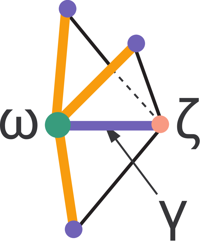
(a)

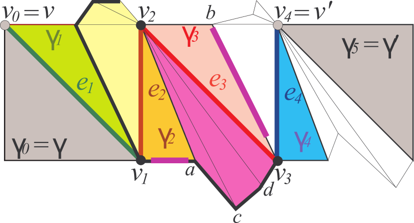
(b)

Figure 3.8: Proof of Property 3.5.1 Part 4 (a) and of Property 3.5.2 (b)

Using the property above, it is easy to prove that a connected combinatorial $d$-manifold is $(d-1)$-connected. This is expressed by the property below that will be useful in the following.

Property 3.5.2.

A combinatorial $d$-manifold is connected if and only if it is $(d-1)$-manifold connected.

Proof 3.5.8.

We have just to prove that a combinatorial $d$-manifold is connected if and only if it is $(d-1)$-connected. In fact, a $(d-1)$-face in a combinatorial $d$-manifold can have up to two cofaces. So, in this context, a $(d-1)$-connected component is also a manifold-connected component.

The easiest way to prove that a combinatorial connected $d$-manifold. is $(d-1)$-connected is by induction on $d$. If $d=1$ the property is obvious. In fact , a complex $\Omega$ it is connected if and only if is $0$-connected (see Section 3.2.3). Let us assume that property holds for connected $h$-manifolds, for $h<d$, and let us prove that it holds for connected $d$-manifolds, too. In Figure 3.8b we show a situation, for $d=2$, which is coherent with the notations chosen in this proof. Let $\gamma$ and $\gamma^{\prime}$ be two $d$-simplices in $\Omega$ (in gray). Let $v$ and $v^{\prime}$ be two Vertices in $\Omega$ (the two gray blobs in figure) such that $v\in\gamma$ and $v^{\prime}\in\gamma^{\prime}$. Being $\Omega$ connected, there exist a path $(v_{i})_{i=0}^{n}$ in $\Omega$, from $v=v_{0}$ to $v^{\prime}=v_{n}$ ($n=4$ in the figure) and such that, for every two consecutive Vertices $v_{i-1}$ and $v_{i}$, the pair $\{v_{i-1},v_{i}\}$ is a $1$-simplex. For each edge $e_{i}=\{v_{i-1},v_{i}\}$ (in green, brown, red and blue) let us select a $d$-coface of $e_{i}$. Let $\gamma_{i}$ be this coface (i.e. $e_{i}\subset\gamma_{i}$). Let us consider the sequence of the $n$ selected $d$-simplices $(\gamma_{i})_{i=1}^{n}$ (in green, brown, pink and pale blue). Let us extend this sequence with $\gamma_{0}=\gamma$ and with $\gamma_{n+1}=\gamma^{\prime}$. We will show that we can insert a $(d-1)$-path between each couple of consecutive $d$-simplices $\gamma_{i}$ and $\gamma_{i+1}$ in the sequence $(\gamma_{i})_{i=0}^{n+1}$. This will create a $(d-1)$-path from $\gamma=\gamma_{0}$ and $\gamma^{\prime}=\gamma_{n+1}$. To do this we note that for any $i=0,\ldots,n$ (we chose $i=2$ in figure), the two consecutive $d$-simplices $\gamma_{i}$ and $\gamma_{i+1}$ share the vertex $v_{i}$. Therefore, both $\gamma_{i}$ ($\gamma_{2}$ in brown) and $\gamma_{i+1}$ ($\gamma_{3}$ in pink) belong to $\star{v_{i}}$ ($\star{v_{2}}$ is made up of eight triangles 3 in yellow one in brown three in violet one in pink). Being $\Omega$ a manifold, we have that $lk(v_{i})$ ($lk(v_{2})$ is the thick black line plus violet $v_{3}b$) is combinatorially equivalent either to the boundary of a $d$-dimensional simplex or to a $(d-1)$-simplex. In both cases, by Property 3.5.1 Part 2, we have that $lk(v_{i})$ is a $(d-1)$-manifold and hence, by inductive hypothesis, $lk(v_{i})$ must be $(d-2)$-connected. We have now that both $\gamma_{i}-\{v_{i}\}$ and $\gamma_{i+1}-\{v_{i}\}$ (edges $v_{1}a$, $v_{3}b$ in violet) belong to $lk(v_{i})$. Therefore, there must be a $(d-2)$-path $(\gamma^{(i)}_{k})$ in $lk(v_{i})$ from $\gamma_{i}-\{v_{i}\}$ to $\gamma_{i+1}-\{v_{i}\}$ (the $0$-path $v_{1}a$, $ac$, $cd$, $dv_{3}$ and $v_{3}b$). Hence, the sequence of complexes $(\{v_{i}\}\bullet\gamma^{(i)}_{k})$ will be a $(d-1)$-path from $\gamma_{i}$ to $\gamma_{i+1}$ (the $1$-path made up of $\gamma_{2}$, $\gamma_{3}$ and the three violet triangles in figure). Therefore, we can build a $(d-1)$-path between any pair of $d$-simplices, $\gamma=\gamma_{0}$ and $\gamma^{\prime}=\gamma_{n+1}$, in the connected $d$-manifold $\Omega$.

A non manifold simplex that is not the face of another non manifold simplex is called a top non manifold simplex.

Remark 3.5.9.

Note that a top non manifold simplex needs not necessarily to be a top simplex. Property 3.5.1 Part 4 implies that a manifold simplex cannot be face of a non-manifold simplex and, hence, all cofaces of a manifold simplex must be manifold simplices.

Example 3.5.2.

Coming back to the example of Figure 3.7a we have that the triangle $poh$ in pale blue is a manifold $2$-simplex since its link is the regular $0$-complex $r$ (in pale blue). This vertex is trivially combinatorially equivalent to the $0$-ball. Similarly the $1$-simplex $rh$ (in red) is a manifold $1$-simplex since its link is the regular $1$-complex $op$ (in red). This is combinatorially equivalent to the $1$-ball. As a direct consequence of Property 3.5.1 Part 4 we have that cofaces of the manifold simplex $rh$ must be manifold simplices. To check this consider $rh$ cofaces i.e. triangles $rph$ and $roh$ and tetrahedron $rohp$. The cofaces of dimension $2$ has links $lk(rph)=o$ and. $lk(roh)=p$. The links $o$ and $p$ trivially satisfy the manifold condition in Definition 3.5.6. Finally we have that the vertex $k$ (in green) is a non-manifold vertex because its link (in green too) is made up of vertex $l$ and of the triangle $rop$ and hence is not regular. As further examples we can look at non-manifold edge $mi$ we can apply Property 3.5.1 Part 4 to see that all faces of $mi$ (i.e. Vertices $m$ and $i$) are non manifold Vertices. Vertices $m$ and $j$ are examples of non-manifold simplices that are not top non-manifold simplices. In turn edge $mi$ is an example of a top non-manifold simplex that is not a top simplex.  

We end this section with a property that will be useful in Chapter 9.

Property 3.5.3.

Let $\Omega$ be a $d$-sphere and let $\gamma$ be a $n$-simplex whose vertices are not in $\Omega$. We have that $\gamma\bullet\Omega$ is a $(d+n+1)$-ball.

Proof 3.5.10.

If $\Omega$ is a $d$-sphere then it is easy to see that the cone $\gamma\bullet\Omega$ is stellar equivalent to the $(d+n+1)$-ball (see for instance [25] Lemma 1.13, Part 2, Pg. 22). This proves that when $\Omega$ is a $d$-sphere then $\gamma\bullet\Omega$ must be a $(d+n+1)$-ball.

3.6 Nerve, Pasting and Quotient space

In this section we introduce the notion of pasting. This notion is sometimes introduced as a tool for the topological classification of closed manifold surfaces (see for instance [45] Pg. 98 and Pg. 222 and [119] Pg.108 and Pg. 152). Indeed, this classification is usually obtained by showing that each closed $2$-manifold can be constructed by pasting a triangulated rectangular sheet at its boundary. Indeed, the result of pasting a complex $\Omega$ onto itself is intimately related with the quotient space for a geometric realizations of $\Omega$ (see [45] Pg. 372). With this idea in mind we report here the basic notions of covering, nerve and of pasting.

Definition 3.6.1 (Covering see [119] Pg. 152 [45] Pg. 61).

A covering of a set $X$ is a collection of subsets of $X$ whose union gives $X$.

Given two coverings ${\mathcal{W}}$ and ${\mathcal{U}}$ we will say that ${\mathcal{W}}$ is a refinement of ${\mathcal{U}}$ (denoted by ${\mathcal{W}}\preceq{\mathcal{U}}$) if there is a function ${\phi}:{\mathcal{W}}\rightarrow{\mathcal{U}}$ such that for each $W\in{\mathcal{W}}$ we have $W\subset\phi(W)$. The function $\phi$ is called a canonical covering projection from ${\mathcal{W}}$ to ${\mathcal{U}}$. In this situation we will say that ${\mathcal{U}}$ is a coarsening of ${\mathcal{W}}$. For coverings of a set $X$ it is easy to see that the relation $\preceq$ is both reflexive and transitive and it is antisymmetric. In the case $X$ is a finite set, the set of coverings of finite set $X$ is a poset ordered by the refinement relation ($\preceq$). A covering whose elements are pairwise disjoint is called a partition. Sets in a partition are called partition blocks.

Given a covering ${\mathcal{U}}$ for a set $X$ we can associate an abstract simplicial complex ${\mathcal{N}}({\mathcal{U}})$ with the covering ${\mathcal{U}}$. The complex ${\mathcal{N}}({\mathcal{U}})$ is called the nerve of the covering ${\mathcal{U}}$. The informal idea behind the concept of the nerve of a covering is better understood if referenced to a less abstract settlement. In fact, let us consider the particular case in which:

• $X$ is a subset of the standard Euclidean space ${\rm I\kern-1.99997ptR}^{n}$ and $X$ is a polyhedron;

• ${\mathcal{U}}$. is a covering of $X$ such that each element in ${\mathcal{U}}$ contains just one vertex from $X$.

In this situation, it is easy to see that the geometric realization of ${\mathcal{N}}({\mathcal{U}})$ can be the polyhedron $X$ For instance it is easy to see that if ${\mathcal{U}}$ is the covering induced by closed faces in a Voronoi diagram, then the associated Delunay triangulation is a possible geometric realization for the nerve ${{\mathcal{N}}({\mathcal{U}})}$. With this idea in mind we can report the definition of nerve (see [119] Pg. 109)

Definition 3.6.2 (Nerve).

Given a covering ${\mathcal{U}}$ of finite set $X$ the nerve of ${\mathcal{U}}$ (denoted by ${{\mathcal{N}}({\mathcal{U}})}$) is the abstract simplicial complex such that:

• the set ${\mathcal{U}}$ is the set of Vertices of ${{\mathcal{N}}({\mathcal{U}})}$ and

• $\gamma=\{v_{1},\ldots,v_{n}\}$ is a simplex in ${{\mathcal{N}}({\mathcal{U}})}$ if and only if  $\cap_{i=1,n}{v_{i}}\neq\emptyset$

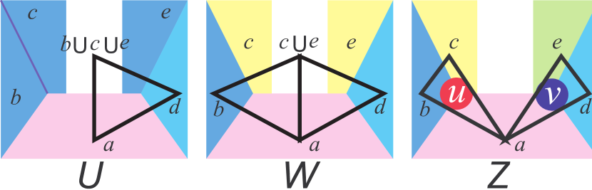
(a)

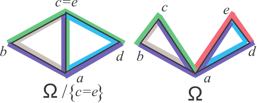
(b)

Figure 3.9: An example of two coverings with the associated nerve (a) and an example of a pasting

Example 3.6.3.

As an example of application of the above definitions consider the three coverings ${\mathcal{U}}$, ${\mathcal{W}}$ and ${\mathcal{Z}}$ for the U shaped domain in Figure 3.9a. Let us concentrate first on the rightmost covering ${\mathcal{Z}}$. The covering ${\mathcal{Z}}$ is made up of the five colored closed polygons $a$ (in pink), $b$ (in blue), $c$ (in yellow), $d$ (in pale blue), and $e$ (in green). Each polygon contains its boundary. It is easy to see that $a$, $b$ and $c$ has a non empty intersection in the vertex $u$ (in red) and $a$, $d$ and $e$ has a non empty intersection in the vertex $v$ (in blue). Therefore the nerve ${\mathcal{N}}({\mathcal{Z}})$ must contain triangles $abc$ and $ade$. It is easy to see that the nerve ${\mathcal{N}}({\mathcal{Z}})$ is exactly the $2$-complex made up of these two triangles.

An abstract simplicial complex $\Omega$ can always be seen as the nerve of a particular covering of $\Omega$. This is expressed by the following property (see Lemma 2.3.13 in [45])

Property 3.6.1.

Let be $\Omega$ an abstract simplicial complex with Vertices in $V$ and let be ${\mathcal{S}}$ the covering of $\Omega$ given by the stars of Vertices in $\Omega$ (i.e. ${\mathcal{S}}=\{\star{v}|v\in V\}$) then $\Omega$ is isomorphic to the nerve ${{\mathcal{N}}({\mathcal{S}})}$

Proof 3.6.4.

To prove this property we note that it can be proved (see Lemma 2.3.13 in [45]) that $\gamma=\{v_{1},\ldots,v_{n}\}$ is a simplex in $\Omega$ if and only if  $\cap_{i=1,n}{\star{v_{i}}}\neq\emptyset$. This happens if and only if  $\{\star{v_{1}},\ldots,\star{v_{n}}\}$ is a simplex in ${{\mathcal{N}}({\mathcal{S}})}$. Therefore the renaming of Vertices ${i}:{V}\rightarrow{\mathcal{S}}$ that sends $v$ into $\star{v}$ is an isomorphism between $\Omega$ and ${{\mathcal{N}}({\mathcal{S}})}$.

We have seen that each abstract simplicial complex can be obtained as a nerve. Similarly there is some relation between the refinement relation between the corresponding coverings and abstract simplicial maps across nerves. More precisely each refinement ${\mathcal{W}}$ of a covering ${\mathcal{U}}$ induce an abstract simplicial map from ${\mathcal{N}}({{\mathcal{W}}})$ to ${\mathcal{N}}({{\mathcal{U}}})$. This is expressed by the following property.

Property 3.6.2.

Let ${\mathcal{W}}$ and ${\mathcal{U}}$ be two coverings such that ${\mathcal{W}}$ is a refinement of ${\mathcal{U}}$ (i.e. ${\mathcal{W}}\preceq{\mathcal{U}}$) and let be ${\phi}:{\mathcal{W}}\rightarrow{\mathcal{U}}$ a canonical covering projection from ${\mathcal{W}}$ to ${\mathcal{U}}$. Then $\phi$ is a vertex map from Vertices of ${\mathcal{N}}({{\mathcal{W}}})$ to Vertices ${\mathcal{N}}({{\mathcal{U}}})$ that induce an abstract simplicial map between the two nerves.

Proof 3.6.5.

See [119] Pg. 152

Following the notation of Property 3.3.2 we have that ${\mathcal{W}}\preceq{\mathcal{U}}$ implies that ${\mathcal{N}}({{\mathcal{U}}})\prec{\mathcal{N}}({{\mathcal{W}}})$.

Example 3.6.6.

The covering ${\mathcal{Z}}$ in Figure 3.9a is an example of a refinement of the covering ${\mathcal{W}}$. In fact the function $[c\mapsto(c\cup e),e\mapsto(c\cup e)]$ is the canonical covering projection ${\phi}:{\mathcal{Z}}\rightarrow{\mathcal{W}}$ such that, for each $Z\in{\mathcal{Z}}$ we have $Z\subset\phi(Z)$. It is easy to see that $\phi$ induce an abstract simplicial map from ${\mathcal{N}}({\mathcal{Z}})$ to ${\mathcal{N}}({\mathcal{W}})$. This map is defined by the vertex map that sends $c$ into $\phi(c)=c\cup e$, and $e$ into $\phi(e)=c\cup e$. Note that $c\cup e$ is a vertex in the nerve ${\mathcal{N}}({\mathcal{W}})$. Similarly, it is easy to see that the covering ${\mathcal{W}}$ is a refinement of the covering ${\mathcal{U}}$ with the canonical covering projection ${\psi}:{\mathcal{W}}\rightarrow{\mathcal{U}}$ given by $\psi=[(c\cup e)\mapsto(b\cup c\cup e),b\mapsto(b\cup c\cup e)]$.

A particular class of nerves is the class of pastings of a complex $\Omega$. Pasting are usually introduced to classify closed $2$-manifolds (e.g. [45]). In this context we use this concept for different goal, namely to investigate the lattice structure in the category of abstract simplicial complexes and abstract simplicial map. The informal idea behind pasting is quite straightforward. Let us consider an abstract simplicial complex $\Omega$ with Vertices in $V$. Given an equivalence relation $R$ on $V$ we can transform complex $\Omega$ into the new complex $\Omega/R$ by pasting together two or more Vertices in $V$ according to $R$. In this context the equivalence relation $R$ is used to specify which Vertices must be identified. We assume that the reader is familiar with the standard terminology for equivalence classes. A short resume is provided in Appendix A Section A.3.

The formal definition of the complex $\Omega/R$ is given considering $\Omega/R$ as the nerve of a particular covering of $\Omega$ induced by $R$.

Definition 3.6.7 (Pasting (see [45] Pg. 222).

Let $\Omega$ be an abstract simplicial complex with Vertices in $V$ and let $R$ be an equivalence relation on $V$. Let $[v]$ be the equivalence class for $v$ induced by $R$ and let $R_{[v]}$ be the set of simplices in $\Omega$ given by the union of open stars of Vertices in $[v]$ (i.e. ${R_{[v]}}=\cup_{w\in[v]}{\star{w}}$). In this situation the complex $\Omega/R$ is defined as the nerve of the covering ${\mathcal{R}}=\{{R_{[v]}}|v\in V\}$.

Note that, for a given equivalence relation $R$, the covering ${\mathcal{R}}=\{{R_{[v]}}|v\in V\}$ is a coarsening of the covering ${\mathcal{S}}=\{\star{v}|v\in V\}$ defined in Property 3.6.1 (i.e. ${\mathcal{S}}\preceq{\mathcal{R}}$). In particular, if we denote with $\Delta_{V}=\{(v,v)|v\in V\}$, the identity relation or the diagonal in $V\times V$ we have that ${\mathcal{S}}={\mathcal{R}}$ if and only if  $R=\Delta_{V}$.

Directly from the Definition 3.6.7 we have that $\Omega/\Delta_{V}$ is isomorphic to $\Omega$ (recall Property 3.6.1 and the fact that $\Omega/\Delta_{V}={\mathcal{N}}({\mathcal{S}})$). Similarly we have that $\Omega/(V\times V)$ is the complex made up of a single isolated vertex. From Property 3.6.2 we have that, for any equivalence $R$ it holds $\Omega/(V\times V)\prec\Omega/R\prec\Omega/\Delta_{V}\cong\Omega$ The relation $R$ will be called the generating relation or the divisor relation for the quotient$\Omega/R$.

Example 3.6.8.

As an example of pasting consider the complex $\Omega$ in Figure 3.9b. We have that $\Omega$ is isomorphic to the nerve ${{\mathcal{N}}({\mathcal{S}})}$ where ${\mathcal{S}}$ is the covering of $\Omega$ given by the stars of Vertices in $\Omega$. In the complex on the right of Figure 3.9b, we have depicted with the same color the edges in each vertex star. For instance, the four blue thick edges belongs to the star of the vertex $a$. The star of each vertex is made up of the two colored thick edges with the triangle between them. The common vertex completes this star. For instance, the star $\star{a}$ is made up of the vertex $a$, of the four edges in blue together with the two triangles $abc$ and $ade$. In the complex on the left of Figure 3.9b we have depicted a coarsening ${\mathcal{S}}^{\prime}$ of the covering ${\mathcal{S}}$. The coarser version ${\mathcal{S}}^{\prime}$ is obtained merging together the stars of $c$ (in green on the right) and of $e$ (in red) into a single item $(\star{c}\cup\star{e})$ (in green on the left). This new item is made up of: the Vertices $c$ and $e$; the four green edges on the left, i.e. $bc$, $ac$, $ae$ and $ed$; the two triangles $abc$ and $ade$. It is easy to see, by exhaustive intersection of elements in ${\mathcal{S}}^{\prime}$, that the complex on the left is isomorphic to the nerve of the covering ${\mathcal{S}}^{\prime}$. We close this example by showing, by Definition 3.6.7, that the nerve ${\mathcal{N}}({{\mathcal{S}}^{\prime}})$ is isomorphic to the pasting $\Omega/R$, with $R$ is the equivalence given by $R=\{(e,c),(c,e)\}$. Indeed, using the notations of Definition 3.6.7, we have $R_{[e]}=R_{[c]}=(\star{c}\cup\star{e})$ while $R_{[v]}=\star{v}$ for all other Vertices $v$. Therefore ${\mathcal{R}}={{\mathcal{S}}^{\prime}}$ and thus $\Omega/R={\mathcal{N}}({{\mathcal{S}}^{\prime}})$.

As we anticipated in the introduction of this section, in the following the complex $\Omega/R$ will be called the quotient of $\Omega$ induced by the relation $R$. We prefer quotient instead of pasting because the abstract simplicial complex $\Omega/R$ is intimately related with the topological quotient space of the geometric realizations of $\Omega$. To state this relation formally we assume that the reader is familiar with the notion of quotient of a topological space $X$ (see [45] Pg. 369 or [119] Pg. 5). Given a topological space $X$ and an equivalence relation $R\subset X\times X$ we will denote with $X/R$ the topological space that is the quotient of $X$ induced by $R$. Assuming this notion we can state the following property.

Property * 3.6.3 (Quotient Geometric Realization).

Let be $\Omega$ an abstract simplicial complex with Vertices in $V$ and let be $R$ an equivalence relation on $V$. Let be $K$ a geometric realization of $\Omega$. In this situation it can be proved that there exist an equivalence relation ${{\bf{p}}(R)}$ over $|K|\times|K|$ such that any geometric realization of the abstract simplicial complex $\Omega/R$ will be homeomorphic to the quotient space $|K|/{{\bf{p}}(R)}$.

Proof 3.6.9.

The proof is sketched in [45] Pg. 372. Here we just report the construction of the equivalence ${{\bf{p}}(R)}$. For each point ${{\bf{q}}}$ in the polyhedrom $|K|$ let be $\{{\bf{q}}_{i}|i=1,\ldots,d+1\}$ the smallest geometric simplex that contains ${\bf{q}}$ and let be $\lambda^{{\bf{q}}}_{i}$ its barycentric coordinates (i.e. ${\bf{q}}=\Sigma_{i=1}^{d+1}{\lambda_{i}^{{\bf{q}}}{\bf{q}}_{i}}$ (see Definition 3.2.2). Let ${\bf{p}}(v)$ be the geometric realization of the vertex $v\in V$ and let ${{\bf{p}}([v])}$ be the set of geometric realization of Vertices in an equivalence class $[v]$ induced by equivalence $R$. Finally we define $\lambda_{[v]}^{{\bf{q}}}$ as the partial sum $\lambda_{[v]}^{{\bf{q}}}=\Sigma_{{\bf{q}}_{i}\in{{\bf{p}}([v])}}{\lambda_{i}^{{\bf{q}}}}$. With this notation the equivalence ${{\bf{p}}(R)}$ is defined by requiring that $({{\bf{q}}},{{\bf{r}}})\in{{\bf{p}}(R)}$ if and only if  $\lambda_{[v]}^{{\bf{q}}}=\lambda_{[v]}^{{\bf{r}}}$ for all the equivalence classes $[v]$ induced by $R$. It is easy to show that the realizations of equivalent Vertices in $R$ are equivalent w.r.t. ${\bf{p}}(R)$ (i.e. ${\bf{p}}(R)\supset\{({\bf{p}}(u),{\bf{p}}(u))|(u,v)\in R\}$) Similarly if ${\bf{q}}$ and ${\bf{r}}$ are two points within the same simplex with barycentric coordinates ${\bf{q}}=\Sigma_{i=1}^{d+1}{\lambda^{{\bf{q}}}_{i}{\bf{q}}_{i}}$ and ${\bf{r}}=\Sigma_{i=1}^{d+1}{\lambda^{{\bf{r}}}_{i}{\bf{r}}_{i}}$ we will have that ${\bf{q}}$ and ${\bf{r}}$ are equivalent in ${\bf{p}}(R)$ whenever, for all $i=1,2,\ldots,(d+1)$, points ${\bf{q}}_{i}$ and ${\bf{r}}_{i}$ are equivalent w.r.t. ${\bf{p}}(R)$ (i.e. $({{\bf{q}}_{i}},{{\bf{r}}_{i}})\in{{\bf{p}}(R)}$ for all $i=1,2,\ldots,(d+1)$ implies that $({{\bf{q}}},{{\bf{r}}})\in{{\bf{p}}(R)}$).

Example 3.6.10.

Returning to the situation of Figure 3.9b we have that equivalence $R=\{(e,c),(c,e)\}$ induce an equivalence ${{\bf{p}}(R)}$. It is easy to see that ${{\bf{p}}(R)}$ is made up of all pairs of geometric Vertices of the form $({{\bf{q}}},{{\bf{r}}})$ and $({{\bf{r}}},{{\bf{q}}})$ such that: point ${{\bf{q}}}$ is in the segment $ac$; point ${{\bf{r}}}$ is in the segment $ae$; points ${{\bf{q}}}$, ${{\bf{r}}}$ have equal barycentric coordinates.

Chapter 4 The Quotient Lattice

4.1 Introduction

There is an obvious relation between abstract simplicial maps and quotients. Indeed a quotient $\Omega^{\prime}/R$ is the image of $\Omega^{\prime}$ via an appropriate abstract simplicial map $f_{R}$. Conversely for each abstract simplicial map  ${f}:{\Omega^{\prime}}\rightarrow{\Omega}$ there exist an appropriate equivalence relation $R_{f}$ such that the image $f(\Omega^{\prime})$ is isomorphic to the quotient $\Omega^{\prime}/R_{f}$. In this chapter we present this relation in detail (in Property 4.2.1) and show that the set of all quotients of a given abstract simplicial complex $\Omega^{\prime}$ form a lattice we called the Quotient Lattice.

The Quotient Lattice is isomorphic to a well known lattice $\Pi_{n}$ called the partition lattice. Mathematical properties of this lattice are given in Appendix A.5. However, in the first part of this chapter, relevant properties are summarized and restated, in an intuitive form, using a language closer to the subject of this thesis.

The quotient lattice, in the context of this thesis, will be used as the structure in which we order the decompositions of a given complex. The relevant factor is that, being this structure a lattice, we can expect to have a least upper bound for any arbitrary set of decompositions. This will be a key issue to define a unique decomposition.

Another key idea in the development of this thesis is the fact that we can manipulate quotients $\Omega^{\prime}/R$ using the set of equations $E$ that defines $R$. In particular, we are interested in the fact that some topological properties can be restated in term of syntactical properties for equations. The manipulation of these syntactical objects will give us an alternative, and sometimes fruitful, way to the treat topological problems. Since these equations identify two vertices together we will call them Stitching Equations. Thus, in this chapter, we finally introduce Stitching Equations and enlight the relation between sets of equations and the Quotient Lattice. Some examples are provided to lead the reader along this path.

4.2 Maps and Equivalence

We start this path with the property below that detals the relation between abstract simplicial maps and quotients $\Omega^{\prime}/R$. In particular parts 1 and 2 further details the structure of the nerve $\Omega/R$ introduced by Definition 3.6.7.

Property 4.2.1.

Let be $\Omega$ an abstract simplicial complex with Vertices in $V$ and let be $R$ and equivalence relation on $V$. In this situation the following properties holds:

1. for any vertex $w$ in $\Omega$ there is a unique vertex $W$ in the nerve $\Omega/R$ such that $\star{w}\subset W$ (or $\{w\}\in W$);

2. A pair of Vertices $u$ and $w$ in $\Omega$ are equivalent w.r.t. $R$ (i.e. $(u,w)\in R$) if and only if  there is a unique vertex $W$ in the quotient $\Omega/R$ such that $\{u\}\in W$ and $\{w\}\in W$;

3. For any quotient $\Omega/R$ we have $\Omega/R\prec\Omega$ and $\Omega/R\cong\Omega$ if and only if  $R=\Delta_{V}$;

4. For any abstract simplicial complex $\Omega\prec\Omega^{\prime}$ there exist an equivalence relation $R_{f}$ such that $\Omega^{\prime}/R_{f}\cong\Omega$;

Proof 4.2.1.

To prove Parts 1 and 2 we proceed as follows. We recall from Definition 3.6.7 that the complex $\Omega/R$ is defined as the nerve of the covering ${\mathcal{R}}=\{{R_{[v]}}|v\in V\}$ with ${R_{[v]}}=\cup_{w\in[v]}{\star{w}}$. Recall also that, in this formula, $[v]$ is the equivalence class for $v$ w.r.t $R$. From the definion of nerve (see Definition 3.6.2) we have that Vertices of $\Omega/R$ are the elements ${R_{[v]}}\in{\mathcal{R}}$. We have that $\{w\}\in\star{v}$ if and only if  $w=v$ and therefore $\{w\}\in{R_{[v]}}$ if and only if  $w\in[v]$. By transitivity we have that $\star{w}\in{R_{[v]}}$ if and only if  $w\in[v]$. We have that $(u,w)\in R$ if and only if  there is a unique equivalence class $[v]$ that contains both $u$ and $w$. This is equivalent to ask to have a unique vertex ${R_{[v]}}$ in $\Omega/R$ such that $\{u\}\in{R_{[v]}}$ and $\{w\}\in{R_{[v]}}$. This proves Part 2. To prove Part 1 we recall that $\star{w}\in{R_{[v]}}$ if and only if  $w\in[v]$. Since equivalence classes are disjoint there must be just one vertex ${R_{[v]}}$ in $\Omega/R$ that contains $\star{w}$. This shows also that there must be just one vertex ${R_{[v]}}$ in $\Omega/R$ that contains $\{w\}$.

To prove Part 3 we proceed as follows. We have seen (see remark after Definition 3.6.7) that $\Omega/R\prec\Omega/\Delta_{V}\cong\Omega$, therefore we just have to prove that $\Omega/R\cong\Omega$ implies $R=\Delta_{V}$. Let us assume that $\Omega/R\cong\Omega$ for some $R\neq\Delta_{V}$ and derive a contradiction. Indeed if the equivalence $R$ is not empty the number of equivalence classes for $R$ is lower that $|V|$ and the covering ${\mathcal{R}}=\{{R_{[v]}}|v\in V\}$ is such that $|{\mathcal{R}}|<|V|$. This leads to a contradiction since $\Omega/R={\mathcal{N}}({{\mathcal{R}}})$ has less Vertices than $\Omega$ and hence cannot be isomorphic to $\Omega$.

To Prove part 4 we proceed as follows. Let $f$ be the map such that $f(\Omega^{\prime})=\Omega$. We define $R_{f}$ to be the equivalence relation such that $(u,v)\in R_{f}$ if and only if  $f(u)=f(v)$. Let $[v]$ be a generic equivalence class w.r.t. $R_{f}$ and let $i$ be the renaming of Vertices ${i}:{\Omega^{\prime}/R_{f}}\rightarrow{\Omega}$ defined by $i({R_{[v]}})=f(v)$. We want to show that $i$ is an isomorphism. We first note that the definition of $i$ is sound since it do not depends on the vertex $v$. Indeed we have that $[u]=[v]$ if and only if  $f(u)=f(v)$. Now we need to show that $i$ maps every simplex in ${\Omega^{\prime}/R_{f}}$ into a simplex of $\Omega$. By Part 3 of this property, we know that there is an abstract simplicial map $g$ that sends $\Omega^{\prime}$ into ${\Omega^{\prime}/R_{f}}$. This is given by the map $g$ defined by $g(v)={R_{[v]}}$. Thus we have that $g(v)={R_{[v]}}$ and we already know that $i({R_{[v]}})=f(v)$. Therefore, for each simplex $\gamma\in{\Omega^{\prime}}$, we can write $i(g(\gamma))=f(\gamma)$. Every simplex in ${\Omega^{\prime}/R_{f}}$ must be of the form $g(\gamma)$, for some $\gamma\in{\Omega^{\prime}}$. Hence, the renaming of Vertices $i$ maps every simplex $g(\gamma)$ in ${\Omega^{\prime}/R_{f}}$ into simplex $i(g(\gamma))=f(\gamma)$. This proves that $i$ is an isomorphism and that $\Omega^{\prime}/R_{f}\cong\Omega$.

In the situation of Property 4.2.1 we will denote with $f_{R}$ the abstract simplicial map ${f_{R}}:{\Omega}\rightarrow{\Omega/R}$ defined as $f_{R}(v)=R_{[v]}$. For any simplex $\gamma\in\Omega$ we use the symbol $\gamma/R$ to denote the simplex that is the image of $\gamma$ in $\Omega/R$ (i.e. $\gamma/R=f_{R}(\gamma)$). We will call $\gamma/R$ the pasted version of $\gamma$ via relation $R$. With some abuse of notation we will denote $\{v\}/R$ with $v/R$. With this notation we can express Part 2 of the previous property by saying that $u/R=v/R$ if and only if  $(u,v)\in R$. Note that $v\in\gamma$ implies that $v/R\in\gamma/R$ while the converse, in general, is false.

4.3 Quotient Lattice

The set of abstract simplicial complexes $\Omega$ with the preorder relation $\Omega\prec\Omega^{\prime}$ is not a poset. As we will see in the following we are interested in finding a least upper bound for certain sets of complexes. Therefore we actually need a poset and a lattice structure. A possible option to construct such a lattice is to identify isomorphic complexes and work with classes of isomorphic complexes (instead of working with plain complexes). In this way, the extension of relation $\prec$ to classes of isomorphic complexes becomes antisymmetric. Furthermore, it is easy to prove that the poset for these classes of isomorphic complexes has a lattice structure.

Unfortunately this choice, although theoretically elegant, leads to an approach that is of limited interest for applications. In fact we should not forget that abstract simplicial complexes are used here to capture the combinatorial structure of a model that still has some geometric realization (see Definition 3.2.4). Thus, the geometric realizations of two isomorphic complexes can be quite different and we could not consider them as equivalent. Thus we need to consider isomorphic and non-identical abstract simplicial complexes as distinct objects.

In the following we will define a lattice that preserve this distinction thus satisfying this basic requirement from the applicative domain. In particular, we will first restrict our attention to quotients of a generic complex $\Omega^{\prime}$ and devise a lattice structure for the set of quotients $\Omega^{\prime}/R$. Later on, in chapter 8, the structure of complex $\Omega^{\prime}$ will be specialized to have all the decompositions of a given complex $\Omega$ as quotients of a certain complex $\Omega^{\prime}$. We will call the lattice of quotients of $\Omega^{\prime}$ the Quotient lattice (for $\Omega^{\prime}$). The quotient  lattice is isomorphic to a well known lattice called the partition lattice. The properties of this lattice, together with the formal background necessary to state them are reported in Appendix A. Here we will use these theoretical tools (i.e. Lattice Theory) in an intuitive fashion. However note that, beyond the informal style of this presentation, examples, properties and definitions are grounded in a sound theoretical framework. We simply make our exposition more intuitive and less formal. A full account on this formal background for $\Pi_{n}$ is given in Section A.5.

The restriction to the lattice of quotients actually do not impair generality. In fact in the quotient lattice for $\Omega^{\prime}$ we have representatives for all complexes that can be obtained modifying $\Omega^{\prime}$. Indeed, we have shown (See forthcoming Property 4.2.1 Part 4) that for any complex $\Omega$ such that $\Omega\prec\Omega^{\prime}$ there exist a quotient $\Omega^{\prime}/R$ isomorphic to $\Omega$. Therefore in the following, in order to study the possible modifications of $\Omega^{\prime}$ we will restrict our attention to the elements in the quotient lattice for $\Omega^{\prime}$. We will study the properties of elements of the form $\Omega^{\prime}/R$ by studying the properties of the relation $R$. This implies that whenever two isomorphic objects $\Omega/R_{1}$ and $\Omega/R_{2}$ are generated by distinct quotients with distinct relations $R_{1}\neq R_{2}$. will be treated as distinct objects.

In order to give here a short account on the partition lattice (see Appendix A) we note that the set of equivalences on $V$ is a poset ordered by the standard set inclusion (i.e. $R_{1}\leq R_{2}$ if and only if $R_{1}\subset R_{2}$). The poset of equivalences on $V$ has a maximum (i.e., the relation $V\times V$) and a minimun (i.e., the identity relation $\Delta_{V}$), being $\Delta_{V}\subset R\subset V\times V$. Then, if $R_{1}$ and $R_{2}$ are two equivalences we define their sum ${R_{1}}+{R_{2}}$ as the smallest equivalence containing the two. Similarly we define their product ${R_{1}}\cdot{R_{2}}$ as the intersection ${R_{1}}\cap{R_{2}}$. Note that the intersection of two equivalences is still an equivalence and is the greatest equivalence contained in them. With these two operations, the poset of equivalences becomes the partition lattice $\Pi_{n}$. In fact sum and product of two equivalence is still an equivalence.

This lattice induce a poset and a lattice over the set of quotients. We called this poset and this lattice respectively the quotient poset and the quotient lattice.

Definition 4.3.1 (Quotient poset).

The set of quotients of a given complex $\Omega^{\prime}$ is a poset with the ordering relation $\leq$ defined as $\Omega/R_{2}\leq\Omega/R_{1}$ if and only if  $R_{1}\subset R_{2}$

By the remark at the end of Property 4.2.1 we have that the mapping that sends $\Omega$ into $\Omega/R$ is injective and thus the quotient poset is anti-isomorphic to the partition lattice $\Pi_{n}$ where $n$ is the number of Vertices in $\Omega$. We recall that two posets are anti-isomorphic if and only if  they are isomorphic but we exchange the direction of the ordering passing from a poset to the other (see Appendix A Section A.2)

The quotient poset has a greatest and a least element. In fact, for any relation $R$ we have: ${\Omega^{\prime}/(V\times V)}\leq\Omega^{\prime}/R\leq\Omega^{\prime}/\Delta_{V}$. Note that the complex $\Omega^{\prime}/\Delta_{V}$ is isomrphic to $\Omega^{\prime}$ (see remark at the end of Definition 3.6.7) while ${\Omega^{\prime}/(V\times V)}$ is the complex made up of single isolated vertex.

The $\leq$ ordering in the quotient  poset implies the preorder given by the relation $\prec$ (associated with abstract simplicial maps). Indeed relations induced by non identical isomorphisms are missing. This connection between these two relations is detailed in the property below.

Property 4.3.1.

Let $\Omega^{\prime}$ be an abstract simplicial complex with Vertices in $V$ and let $R_{1}$ and $R_{2}$ be two equivalence relations on $V$. In this situation if $\Omega^{\prime}/R_{2}\leq\Omega^{\prime}/R_{1}$ then $\Omega^{\prime}/R_{2}\prec\Omega^{\prime}/R_{1}$

Proof 4.3.2.

To Prove this property we proceed as follows. Since $\Omega^{\prime}/R_{2}\leq\Omega^{\prime}/R_{1}$ we have that $R_{1}\subset R_{2}$. Let $[v]_{1}$ and $[v]_{2}$ the equivalence classes of $v$ w.r.t., respectively, $R_{1}$ and $R_{2}$. We have that $[v]_{1}\subset[v]_{2}$ for all $v\in V$ if and only if  $R_{1}\subset R_{2}$. Since we have that $[v]_{1}\subset[v]_{2}$ for all $v\in V$ we can say that the covering ${\mathcal{R}}_{1}=\{{R_{[v]_{1}}}|v\in V\}$ is a refinement of ${\mathcal{R}}_{2}=\{{R_{[v]_{2}}}|v\in V\}$. Finally, by Property 3.6.2, we have that $\Omega^{\prime}/R_{2}\prec\Omega^{\prime}/R_{1}$

It is easy to see that, the situation of Property 4.3.1 (whenever $R_{1}\subset R_{2}$, we have that Vertices in $\Omega^{\prime}/R_{2}$ are obtained as union of Vertices from $\Omega^{\prime}/R_{2}$, in particular we have that ${R_{[v]_{2}}}=\cup_{u\in[v]_{2}}{R_{[u]_{1}}}$. We note that the converse is not true, in particular there exist pairs of isomorphic quotients $\Omega/R_{2}$ and $\Omega/R_{1}$ for which $\Omega/R_{2}\prec\Omega/R_{1}$ and $\Omega/R_{1}\prec\Omega/R_{2}$ and neither $R_{1}\subset R_{2}$ nor $R_{2}\subset R_{1}$ (i.e. neither $\Omega/R_{2}\leq\Omega/R_{1}$ nor $\Omega/R_{1}\leq\Omega/R_{2}$). In the next example we present one of these situations.

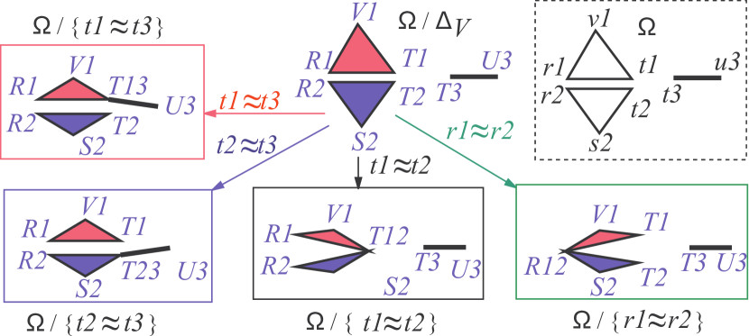
Figure 4.1: An example of a poset of quotients

Example 4.3.3.

As an example of application of the definitions above consider Figure 4.1. In Figure 4.1 we sketched a portion of the poset of quotients $\Omega/R$. The complex $\Omega$ (in the dashed frame on the top right) is the $2$-complex made up of the two triangles $r1v1t1$, $r2v2t2$ and of the segment $t3u3$ . We recall that Vertices in the quotient complex $\Omega/R$ are collection of simplices and, for sake of clarity, we used for this collection a label of the form $Xn$ (i.e. V1 R1 etc.). These labels are chosen following a certain convention. Label $Vn$ is used for vertex $R_{[vn]}$ in the quotient $\Omega/\Delta_{V}$. Note that vertex $Vn$ is a set of simplices from $\Omega$ (see Definition 3.6.2 and 3.6.7). Label $Rxy$ is used for vertex $R_{[rx]}\cup R_{[ry]}$ and similarly label $Txyz$ (in forthcoming examples) will be used for vertex $R_{[tx]}\cup R_{[ty]}\cup R_{[tz]}$.

With these assumption we can use the annotated Hasse diagram of Figure 4.1 to show the application of Property 4.2.1 and of Property 4.3.1 (see Section A.2 in Appendix A for a definiton of Hasse diagram). For our convenience we used arrows that are not provided by standard Hasse diagrams. Here and in the following we use the notation $\{t1\approx t2\}$ to denote the smallest equivalence that contains $(t1,t2)$.

A first thing to note is this. If an arrow exist from the $\Omega/R_{1}$ to $\Omega/R_{2}$ then it must be $R_{2}\subset R_{1}$. Consider for instance the complex $\Omega/\Delta_{V}$ and the complex we labeled with $\Omega/\{t1\approx t2\}$. This complex can be obtained by stitching together the two triangles in $\Omega/\Delta_{V}$ at $t1$ and $t2$. Looking at vertex labels in the quotient $\Omega/\{t1\approx t2\}$ we can verify what stated in Property 4.2.1 Part 2. In fact all Vertices in $\Omega/\Delta_{V}$ remains unchanged in $\Omega/\{t1\approx t2\}$ but Vertices labeled $T1$, $T2$ that maps to $T12$.

According to the notation introduced at the end of Property 4.2.1 we have that simplex $R2T23$ can be denoted as $r2t2/\{t2\approx t3\}$.

In this figure each arrow denotes the application of the abstract simplicial map foreseen by Property 4.3.1. If an arrow is labeled with equation $vx\approx vy$ it is easy ot see that the abstract simplicial map  is induced by the vertex map $[Vx,Vy\mapsto Vxy]$. Arrows in this diagram represent the abstract simplicial maps foreseen by Property 4.3.1 since trivially, for any relation $R$, we have $\Omega/R\leq\Omega/\Delta_{V}$.

Finally note that the four non trivial quotients are pairwise isomorphic. For instance quotient $\Omega/\{t_{1}\approx t3\}$ and $\Omega/\{t_{2}\approx t3\}$ are isomorphic and no inclusion holds between the generating relations $\{t1\approx t3\}$ and $\{t2\approx t3\}$.

The quotient poset becomes a lattice with the two operations $\uparrow$ (sum or join) and $\downarrow$ (product or meet) defined by:

$$(\Omega^{\prime}/{R_{1}})\downarrow(\Omega^{\prime}/{R_{2}})=\Omega^{\prime}/({{R_{1}}+{R_{2}}})\hskip 28.45274pt(\Omega^{\prime}/{R_{1}})\uparrow(\Omega^{\prime}/{R_{2}})=\Omega^{\prime}/({{R_{1}}\cdot{R_{2}}})$$

We will call this lattice the quotient lattice. This is anti-isomorphic w.r.t. the partition lattice $\Pi_{n}$.

We found convenient to use arrows for lattice operators $\downarrow$ and $\uparrow$ to support intuition. Indeed, according to the usual convention in Hasse diagrams (see Appendix A Section A.2) of having greater elements up we found convenient to use the symbol $\downarrow$ for the meet since this is the greatest lower bound. Similarly we choose the symbol $\uparrow$ for the join because this is the least upper bound. Note that in the Appendix A the basic results about Lattice Theory are reported using the more usual convention where the sum or join $\uparrow$ is represented by the ${\vee}$ symbol.

We recall that $\Omega^{\prime}\prec\Omega^{\prime\prime}$ if and only if there exist a abstract simplicial map $f$ such that $\Omega^{\prime}=f(\Omega^{\prime\prime})$. Therefore, we defined the sense of order $\prec$ to be graphically coherent with arrow for $f$. The abstract simplicial maps goes from greater elements to smaller elements w.r.t. $\prec$ and $A\prec B$ intuitively reads as A is less exploded than B or B is more detailed than A.

Note that passing from equivalences to complexes we have two corresponding but opposite orders. As a consequence the sum of two equivalences ${{R_{1}}+{R_{2}}}$ gives the product (meet) among complexes $(\Omega/{R_{1}})\downarrow(\Omega/{R_{2}})$. Similarly the product of two equivalences ${{R_{1}}\cdot{R_{2}}}$ gives the sum (join) among complexes $(\Omega/{R_{1}})\uparrow(\Omega/{R_{2}})$. Sometimes, in next sections, we will prefer to use $\Omega/({{R_{1}}+{R_{2}}})$ and $\Omega/({{R_{1}}\cdot{R_{2}})}$, instead of as $(\Omega/{R_{1}})\uparrow(\Omega/{R_{2}})$ and $(\Omega/{R_{1}})\downarrow(\Omega/{R_{2}})$ being usually interested in the operations on the equivalences that are behind the operations $\uparrow$ and $\downarrow$.

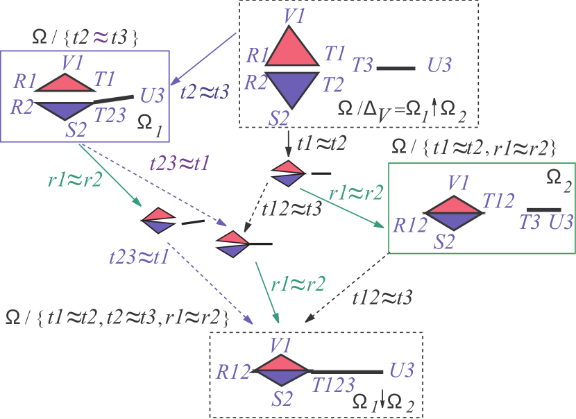
Figure 4.2: An example of portion of a lattice of quotients

Example 4.3.4.

In Figure 4.2 we present another portion of the poset of Figure 4.1. In this second figure we extend the form of arrow labels using also labels of the form $vxy\approx vz$. This means that the corresponding one hop abstract simplicial map is induced by the vertex map $[Vx,Vy,Vz\mapsto Vxyz]$. This second figure shows an instance of two lattice operations, $\Omega_{1}\uparrow\Omega_{2}$ and $\Omega_{1}\downarrow\Omega_{2}$, between the two quotients $\Omega_{1}=\Omega/\{t2\approx t3\}$ and $\Omega_{2}=\Omega/\{r1\approx r2,1\approx t2\}$. We note that we have just one hop from $\Omega_{1}\uparrow\Omega_{2}$ to $\Omega_{1}$ and just one hop from $\Omega_{2}$ to $\Omega_{1}\downarrow\Omega_{2}$. This proves that these two complexes are, respectively, the least upper bound and the greatest lower bound for the pair $\{\Omega_{1},\Omega_{2}\}$. In this figure we used the notation $\{t1\approx t2,t2\approx t3,r1\approx r2\}$ to denote the smallest equivalence that equates $t1$ with $t2$ and $t3$ and $r1$ with $r2$. If we consider the two relations generating $\Omega_{1}$ and $\Omega_{2}$ (i.e. $\{t2\approx t3\}$ and $\{t1\approx t2,r1\approx r2\}$), then it is easy to verify that the least upper bound and the greatest lower bound for the pair $\{\Omega_{1},\Omega_{2}\}$ are given respectively by the quotient of $\Omega$ with the intersection (i.e. $\Delta_{V}=\{t2\approx t3\}\cap\{t1\approx t2,r1\approx r2\}$) and with the sum (i.e. $\{t1\approx t2,t2\approx t3,r1\approx r2\}$) of the two equivalence relations generating $\Omega_{1}$ and $\Omega_{2}$.

We have shown that the quotient lattice and the lattice of equivalences are anti-isomorphic. It is quite easy to see that the set of simplices in an abstract simplicial complex $\Omega$, ordered by set inclusion, is a lattice, too. This lattice is usually called the face lattice $\Omega$. Lattice operations for this lattice are usual set theoretic union (join) and intersection (meet). This explain why the name join is used for the operation $\gamma_{1}\bullet\gamma_{2}$. However note that the join $\gamma_{1}\bullet\gamma_{2}$ from Combinatorial Topology is a partial version of the join in the face lattice. In fact $\gamma_{1}\bullet\gamma_{2}$ undefined whenever $\gamma_{1}\cap\gamma_{2}\neq\emptyset$.

The quotient operation is linear w.r.t. operations in the face lattice, More precisely the following identities holds:

Property 4.3.2.

Let $\gamma_{1}$ and $\gamma_{2}$ be two simplices in the abstract simplicial complex $\Omega$. Let $V$ be the set of vertices in $\Omega$ and let $R$ be an equivalence relation on $V$. In this situation the following identites holds:

$$\frac{\gamma_{1}}{R}\cup\frac{\gamma_{2}}{R} = \frac{\gamma_{1}\cup\gamma_{2}}{R}$$ (4.1)

$$\frac{\gamma_{1}}{R}\cap\frac{\gamma_{2}}{R} = \frac{\gamma_{1}\cap\gamma_{2}}{R}$$ (4.2)

$$\gamma_{1}\leq\gamma_{2} \Rightarrow \frac{\gamma_{1}}{R}\leq\frac{\gamma_{2}}{R}$$ (4.3)

In this framework we are interested also in the extension of the quotient notation (i.e. $\Omega/{\approx}$) to the composition of two or more equivalences in $V\times V$. Note that if $\approx_{1}$ and $\approx_{2}$ are two relations in $V\times V$ the composition of two quotients $(\Omega/{\approx_{1}})/{\approx_{2}}$ is undefined. Indeed, using the previous definitions, we can attach a meaning to $(\Omega/{\approx_{1}})/{\approx_{2}}$ if and only if  the relation $\approx_{2}$ is a relation among Vertices of $\Omega/{\approx_{1}}$. This is not used at all and, usually, both $\approx_{1}$ and $\approx_{2}$ are relations between the Vertices of $\Omega$. In this latter situation we use the notation $(\Omega/{\approx_{1}})/{\approx_{2}}$ after the following definitions.

Definition 4.3.5.

Let $\Omega$ be an abstract simplicial complex with Vertices in $V$ and let $\gamma$ be a simplex in $\Omega$. Let $\approx_{1}$ and $\approx_{2}$ be two relations in $V\times V$ (i.e. .$\approx_{1}\subset V\times V$ and $\approx_{2}\subset V\times V$). In this situation we define:

$$\begin{array}[]{ccccc}(\Omega/{\approx_{1}})/{\approx_{2}}&=&\Omega/({\approx_{1}}+{\approx_{2}})&=&(\Omega/{\approx_{2}})/{\approx_{1}};\\ (\gamma/{\approx_{1}})/{\approx_{2}}&=&\gamma/({\approx_{1}}+{\approx_{2}})&=&(\gamma/{\approx_{2}})/{\approx_{1}};\end{array}$$

4.4 Stitching Equations

We close this chapter with a discussion on the relation between equivalence and sets of equations. We already used equations (e.g. $\{t2\approx t3\}$) in examples. In this section we will study the relation between equations and the structure of the quotient lattice. Indeed the partition lattice, and so the lattice of equivalences and the quotient lattice, belongs to a special class of lattices called geometric lattices. The basic property of a finite geometric lattice is that each element in a geometric lattice can be expressed as the join of a finite number of a set of generators called points. Thus, for the lattice of equivalence relations the points are those equivalence relations that are generated by a single equation ‘(e.g. $\{t2\approx t3\}$). Obviously, in this thesis, we do not call them points to avoid confusion with the Vertices in abstract simplicial complex. We recall that an abstract simplicial complex $\Omega$, ordered with the face relations is a lattice called the face lattice. The face lattice is geometric lattice, too and $0$-simplices $\{v\}$ in $\Omega$ are the points for this lattice. A short introduction to these concepts is in Section A.5 of Appendix A.

In the following we will use expressions of the form $u\approx v$, called stitching equations, to denote the smallest equivalence that contains the couple $(u,v)$. As a consequence $u\approx v$ and $v\approx u$ will denote the same object. We will say that the equivalence ${\approx}\subset V\times V$ satisfies the equation $u\approx v$ if and only if $(u,v)\in{\approx}$. We will write $u\not\approx v$ if and only if $(u,v)\not\in{\approx}$. In this case we will say that the equivalence $\approx$ do not satisfies the equation $u\approx v$. An equivalence $\approx$ is usually given by a set of equations of the form $E=\{u_{i}\approx v_{i}|i=1,\ldots k\}$. The equivalence given by such a set of equations $E$, denoted by $\approx^{E}$, is the the smallest equivalence $\approx^{E}$ such that $\approx^{E}$ satisfies all the equations in $E$. (i.e. $u_{i}\approx^{E}v_{i}$ for $i=1,\ldots,k$). We will say that $E$ denotes or generates $\approx^{E}$

If $E$ is a set of equations that generates a an equivalence, denoted by $\approx^{E}$, we will use $E$ as a shortcut for $\approx^{E}$ in all the expressions where this is not ambiguous. In particular we will write $\approx+\;E$ and $\approx\cdot\;E$ as a shortcut for $\approx+\approx^{E}$ and $\approx\cdot\approx^{E}$. Similarly we will use $\Omega/E$ as a shortcut for $\Omega/{\approx^{E}}$ and $\gamma/E$ as a shortcut for $\gamma/\approx^{E}$.

4.4.1 Independent Equations

We can generate an equivalence using several sets of equations. However there exists sets of equations that are, in some sense, redundant. The concept of redundancy is perfectly captured by the specific notion of independence in geometric lattices. In this subsection we will adapt this notion to our particular framework and report the related results (without proof). Section A.4 in the Appendix A and in particular the material following Definition A.4.4 discuss the general notion of independence in geometric lattices and lists the related results.

A set of equations $E$ is redundant if the equivalence $\approx^{E}$ can be generated by a subset of $E$. A non redundant set of equations is called a set of independent equations. All non redundant sets of equations that generates the same equivalence contains the same number of equations. This number is called the rank index of the equivalence. If ${\approx_{2}}$ is the immediate superior of $\approx_{1}$ then there exist an equation $u\approx v$ s.t. $u\not\approx_{1}v$ and ${\approx_{1}}+{\{u\approx v\}}={\approx_{2}}$. In this case we will say that ${\{u\approx v\}}$ labels the one hop chain from ${\approx_{1}}$ to ${\approx_{2}}$ (or from $\Omega/{\approx_{2}}$ to $\Omega/{\approx_{1}}$). Longer chains will be labeled by sequences of independent equations. Note that same chain can be labeled by different labels and the same label can be used to label different chains in the quotient lattice.

In general some care must be taken not to overlook this analogy between complexes, equivalences and equations. Indeed there is not a one to one correspondence between set of equations and equivalences. So, for instance, $\approx^{E_{1}}=\approx^{E_{2}}+\approx^{E}$ (that can also be written as $E_{1}=E_{2}+E$) do not implies that $E_{1}=E_{2}\cup E$

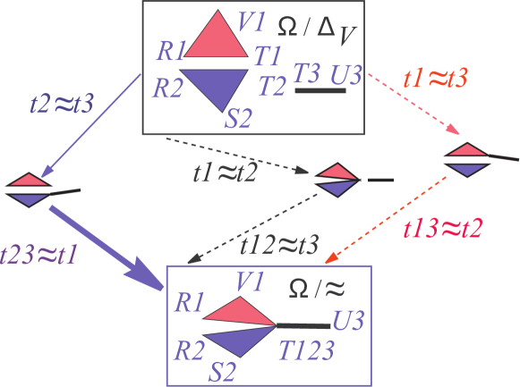
Figure 4.3: Different sets of equations can generate equivalence $\approx$ in $\Omega/{\approx}$ (See Example 4.4.1)

Example 4.4.1.

Note that different sets of equations can be associated to the equivalence $\approx$. Let us consider the portion of the quotient lattice in Figure 4.3. In this figure we use the label $vxy\approx vz$ to say that the corresponding one hop path can be labeled either with $vx\approx vz$ or by $vy\approx vz$. Looking at the three paths (solid or dashed) in Figure 4.3 we have that several pairs of equations can be used to generate the equivalence $\approx$. According to the labeling conventions we can build a set of equations for $\approx$ by collecting equations that labels the one hop steps in the Hasse diagram of Figure 4.3. We just have to collect labels on a path from $\Omega/\Delta_{V}$ down to $\Omega/{\approx}$. Following the solid path we can take $E=\{t1\approx t3,t3\approx t2\}$ or $E^{\prime}=\{t1\approx t3,t1\approx t2\}$ and still have ${\approx}={\approx^{E}}={\approx^{E^{\prime}}}$. These two variants are obtained since, from the second (thick) solid arrow, we can get either equation $t3\approx t2$ or equation $t1\approx t2$. The same sets comes from the two dashed paths on the right of Figure 4.3. Following this path we always collect one of the two sets $E$ or $E^{\prime}$. This fact is a consequence of a general property of geometric lattices called semimodularity. This property will be introduced in the following subsection.

Finally, as an example of application of Definition 4.3.5, we note that following the solid path we can write $\Omega/{\approx}$ as $(\Omega/\{t1\approx t3\})/\{t1\approx t2\}$.

4.4.2 Semimodularity

Although, different labels are possible for a path, even for a one hop path (see, for instance, the solid thick edge in Figure 4.3), nevertheless, we have that the size of the set of independent equations that labels a path must be constant. In general, let us consider two a starting point $\Omega/{\approx^{E_{x}}}$ and an ending point $\Omega/{\approx^{E_{y}}}$ (or shortly $\approx^{E_{x}}$ and $\approx^{E_{y}}$) we can collect different labels traveling through different paths from $\approx^{E_{x}}$ to $\approx^{E_{y}}$. However, we always have the option to collect the same labels (i.e. the same unordered set of equations) traveling through different paths from $\approx^{E_{x}}$ to $\approx^{E_{y}}$. This is a consequence of a general property for geometric lattices called semimodularity. Semimodularity is formally introduced in Appendix A Section A.5, Definition A.4.3. In the Appendix, together with semimodularity definition, we list relevant properties for semimodular latices. The partition lattice $\Pi_{n}$, being a geometric lattice, is semimodular. Thus the quotient lattice, being anti-isomorphic w.r.t. the partition lattice, is semimodular, too.

In this framework semimodularity gives us an interesting property for labels, (and for equations). In fact, in general, extending the construction of the diagram of Example 4.4.1 to a larger portion of the quotient lattice one can prove that, given two equivalences $E_{a}$ and $E_{b}$ (note we use $E_{a}$ as a shorthand for $\approx^{E_{a}}$) with a common upper bound $E_{x}$ and a common lower bound $E_{y}$ we can use the same label $E_{xa}$ for the chain from $E_{x}$ to $E_{a}$ and for the chain from $E_{b}$ to $E_{y}$. Similarly we can use the same label $E_{xb}$ for the chain from $E_{x}$ to $E_{b}$ and for the chain from $E_{a}$ to $E_{y}$. With reference to the situation depicted in the following diagram we can say that semimodularity ensures that parallel arrows can receive the same labeling :

 

 $$E_{x}$$

  ΓΓΓΨ      @@R

 

  @@R      ΓΓΓΨ

 

 

Example 4.4.2.

As an example of application of semimodularity consider the poset in Figure 4.4. This is generated taking all the one hop steps that leaves from $\Omega/\Delta_{V}$ and its successors. Arrows received different colors and were depicted dashed or not. A table at the bottom of the figure gives labels for all the arrows types. We can use colors in this diagram to verify that two paths with a common start and common end can be labeled by the same set of equations. First note that dashed arrows can be labeled with a couple of equations. For instance dashed black arrows can be labeled with equation $t1\approx t3$ or with equation $t2\approx t3$. Solid arrows can be labeled with only one equation. Coloring for solid arrows is chosen so that red, blue and black dashed arrows can be labeled only with an equation that labels solid arrows of the other two colors in the triple red blue and black. Green do not participate to this scheme. For instance dashed black arrows can be labeled with equations that are on solid red and blue arrows (i.e. $t1\approx t3$ and $t2\approx t3$).

To check semimodularity in this tiny example we have to select two paths with a common start and a common end. Next we label them and see if semimodularity holds. That’s to say, we compare the two paths to see if they can be labeled with the same set of equations. So, for instance, if we compare two paths and in one we have a black dashed arrow then, in the other path, we must have a red or blue solid arrow. We can say that a black dashed arrow can be balanced by a red or blue solid arrow. Similarly we will say that a red dashed arrow can be balanced by a black or blue solid arrow. Finally a black or red solid arrow will balance a blue dashed arrow. Green solid arrows can only be balanced by another green solid arrow. With these remarks in mind we can travel, for instance, from $\Omega/\Delta_{V}$ down to $\Omega/\{t1\approx t2,t2\approx t3,r1\approx r2\}$ and see if the colors we collect balance. Note that others starting and ending points are possible, too. For this top to bottom travel, for instance, we can go down via the leftmost path i.e. red arrow, next dashed red and finally green arrow. Another path, that balances this, is, for instance, the rightmost i.e. green, black and dashed black. Indeed, in the two paths we have two greens that balance each other, then red balance dashed black and dashed black balance with solid red. Note that in this drawing things are organized so that parallel arrows balances so one can easily see that semimodularity holds.

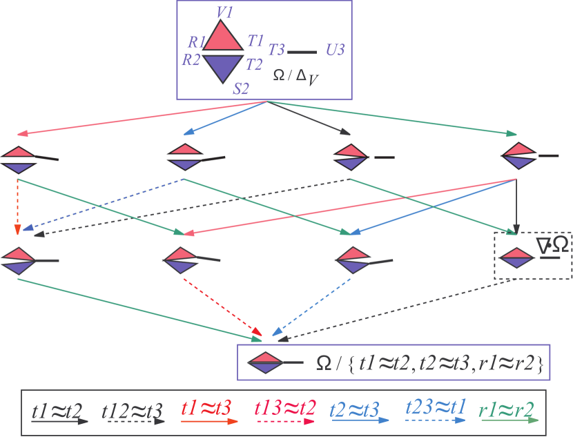
Figure 4.4: Semimodularity in the quotient lattice (See Example 4.4.2). The complex $\nabla\cdot{\Omega}$ is the standard decomposition of the complex at the bottom of the lattice. This complex is framed for future reference (see Chapter 8)

Closing this section we like to stress the fact that the main consequence of semimodularity is that stitching equations actually provides a powerful abstraction to denote transformation between simplices. This is especially true if we compare them against equivalences. Indeed an equivalence is a global object whose form heavily depends on (the set of vertices of) the complex it applies to. Sets of equations, on the contrary, do not depend on a particular complex and can be used to label paths between different complexes. Each equation actually defines some sort of rewrite rule whose effect is local and independent from the global context in which it is applied. Thus stitching equations are the right basic tool to denote a transformation between complexes. Indeed, as we will see, stitching equations are too basic for our needs because they impose a too fine grained view on the quotient lattice. To correct this problem, in Chapter 6 we will introduce simplex gluing instructions as a means to group together stitching equations into more complex transformations.

Chapter 5 Decomposition Lattice

5.1 Introduction

Obviously not all the quotients $\Omega=\Omega^{\prime}/E$ of a given complex $\Omega^{\prime}$ are such that $\Omega^{\prime}$ is a decompositions of $\Omega$. For instance, by equation $E=\{a\approx b\}$ we can readily collapse a triangle $abc$ into one of its edges $ac$ and an edge is not the decomposition of a triangle. Thus, in this chapter, we will characterize the set of equivalences $R$ that makes $\Omega^{\prime}$ a a decomposition of the quotient $\Omega=\Omega^{\prime}/R$. Intuitively, a complex $\Omega^{\prime}$ is a decomposition of $\Omega$ if pasting together pieces of $\Omega^{\prime}$ we can obtain $\Omega$. Furthermore, we expect that nothing shrinks or collapse passing from $\Omega^{\prime}$ to $\Omega$. More precisely intuition require to have a dimension preserving bijection between top simplices in $\Omega^{\prime}$ and $\Omega$. In this chapter we define the notion of decomposition and identify a sublattice of a particular quotient lattice that we called the decomposition lattice. This lattice contains an isomorphic copy for any decomposition of a given complex $\Omega$.

5.2 Decompositions

We first define the notion of decomposition using abstract simplicial maps. In the next section we will restrict our attention to a particular class of decompositions that form a lattice and that contains an isomorphic representative for each decomposition of a given complex. We recall that, by Property 4.2.1 Part 3, there is an abstract simplicial map  associated with each equivalence $\approx$.

Definition 5.2.1 (Decomposition).

An abstract simplicial complex $\Omega^{\prime}$ is a decomposition of $\Omega$ if and only if  ${\Omega^{\prime}/{\approx}}\cong\Omega$ and the abstract simplicial map from $\Omega^{\prime}$ to $\Omega^{\prime}/{\approx}$ is a dimension preserving map that induces a bijection between top simplices.

In the following we will introduce the lattice of the possible decomposition of $\Omega$ called the decomposition lattice of $\Omega$. The decomposition lattice is a sublattice of the quotient lattice for a particular complex $\Omega^{\top}$ that we will obtained as the total decomposition of $\Omega$. We called this complex the totally exploded decomposition of $\Omega$. In the rest of this thesis we will consider only decomposition in the decomposition lattice. This restriction do not impairs the generality of the approach. In fact, we will show that (see Property 5.4.2), for any decomposition $\Omega^{\prime\prime}$, there exists at least a decomposition in the decomposition lattice that is isomorphic to $\Omega^{\prime\prime}$.

5.3 The totally exploded decomposition $\Omega^{\top}$

We start the construction of the decomposition lattice with the definition of the totally exploded decomposition of a complex $\Omega$. This will be denoted by $\Omega^{\top}$. We can intuitively define the totally exploded decomposition of $\Omega$ by saying that $\Omega^{\top}$ is the decomposition of $\Omega$ where each top simplex in $\Omega^{\top}$ is a distinct connected component. This requirement completely defines $\Omega^{\top}$ up to isomorphism. It is easy to see that the top simplices in $\Omega^{\top}$ must be the same, for number and dimension, as those in $\Omega$. For instance in Figure 5.1a complex $\Omega^{\top}$ (on the right) is the totally exploded version of complex $\Omega$ (on the left).

The intuitive definition of $\Omega^{\top}$ do not identify clearly the complex $\Omega^{\top}$. Indeed countably many different isomorphic options exist for the choice of $\Omega^{\top}$. To make both theory and proofs straightforward we chose a particular naming for Vertices in $\Omega^{\top}$. Let $\Theta$ be the set of top simplices in $\Omega$, then, for each top simplex $\theta=\{u,v,w,\ldots\}$, we will place in $\Omega^{\top}$ the simplex $\theta^{\top}=\{u_{\theta},v_{\theta},w_{\theta},\ldots\}$. The above conventions leads to the following definition.

Definition 5.3.1 (Totally Exploded Decomposition).

Let be $\Theta$ the set of top simplices in $\Omega$. We will define the totally exploded decomposition of a complex $\Omega$, denoted by $\Omega^{\top}$, as the complex whose set of top simplices is $\Theta^{\top}=\{\theta^{\top}|\theta\in\Theta\}$ with $\theta^{\top}=\{v_{\theta}|v\in\theta\}$.

We will denote with $V^{\top}$ the set of Vertices in $\Omega^{\top}$. It is easy to see that there is a distinct vertex $v_{\theta}$ in $V^{\top}$ for each vertex $v\in V$ and for each top simplex $\theta$ in the star of $v$. Hence we have $V^{\top}=\{v_{\theta}|v\in V\,\,{\rm and}\,\,\theta\in star({v},{\Omega})\cap\Theta\}$.

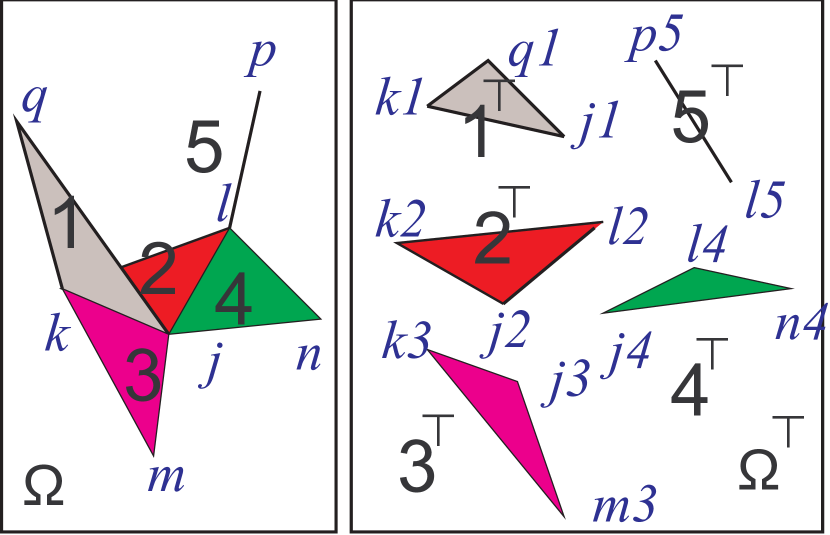
(a)

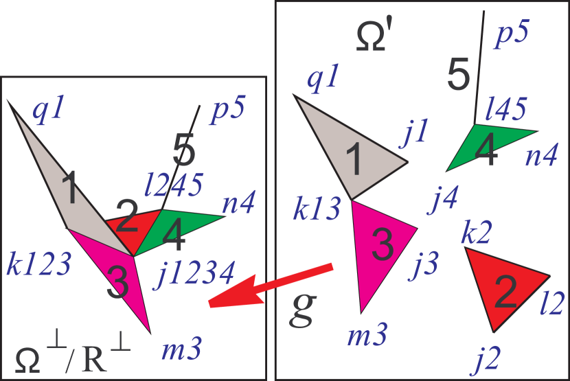
(b)

Figure 5.1: Example of totally exploded decomposition (a) (see Definition 5.3.1) and of $\Omega^{\top}/R^{\top}$ (b) (see Property 5.3.1).

Example 5.3.2.

Consider for instance the complexes in Figure 5.1a. To enhance readability we have labeled top simplices in $\Omega$ with integers. We used the label $1$, for instance, as a shortcut for the simplex $\theta_{1}=\{k,q,j\}$ (we recall that in an abstract simplicial complex a $d$-simplex is a set of $d+1$ Vertices). Similarly, we have labeled Vertices in $\Omega^{\top}$ with alphanumeric strings of the form $vx$ where $v$ is a vertex of $\Omega$ and $x$ is the number that labels a simplex. The label $vx$ stands for the vertex name $v_{\theta_{x}}$. Note that, for instance, label $k1$ stands for $k_{\theta_{1}}$ that, in turn must be unfolded as $k_{\{k,q,j\}}$. For obvious reasons in examples we will use shortcuts as $k1$ instead of this heavy notation. Similarly the label $1^{\top}$ is a shortcut for the simplex $\theta_{1}^{\top}=\{k,q,j\}^{\top}=\{k1,q1,j1\}$. Unfolding shortcuts we can write $\theta_{1}^{\top}=\{k_{\theta_{1}},q_{\theta_{1}},j_{\theta_{1}}\}$ that in turn, by unfolding $1$ becomes $\{k_{\{k,q,j\}},q_{\{k,q,j\}},j_{\{k,q,j\}}\}$. With these conventions we have that the complex $\Omega^{\top}$ on the right of Figure 5.1a is the totally exploded version of $\Omega$ with Vertices chosen according to the conventions described above.

We can stitch together top simplices from $\Omega^{\top}$ and obtain a range of decomposition of $\Omega$ reaching, in the end, $\Omega$ itself. This range of decomposition will be our decomposition lattice. A first step towards the definition of this lattice is the following property that sets top and bottom elements for the decomposition lattice.

Property 5.3.1.

The complex $\Omega^{\top}$ is a decomposition of $\Omega$ and there exist an equivalence $R^{\top}$ such that ${\Omega^{\top}/R^{\top}}\cong\Omega$. The equivalence $R^{\top}$ is unique up to isomorphism.

Proof 5.3.3.

In the situation of the definition 5.3.1 the vertex map ${f}:{\Omega^{\top}}\rightarrow{\Omega}$ defined by $f(v_{\theta})=v$ induce a dimension preserving abstract simplicial map that is a bijection between top simplices that maps simplex $\theta^{\top}$ into $\theta$ and $f(\Omega^{\top})=\Omega$. The map $f$ is uniquely identified by these conditions. We recall that, by Property 4.2.1 Part 3, there is a unique abstract simplicial map associated with each equivalence. Let $R_{\top}$ be the equivalence associated with the abstract simplicial map $f$. By Part 4 of Property 4.2.1 we have that ${\Omega^{\top}/R^{\top}}\cong\Omega$. Therefore there exist an isomorphism $i$ from ${\Omega^{\top}/R^{\top}}$ to $\Omega$. Composing $i$ with $f$ we obtain a dimension preserving abstract simplicial map between $\Omega^{\top}$ and $\Omega$. This proves that $\Omega^{\top}$ is a decomposition.

As an example of application of these concepts consider the following example.

Example 5.3.4.

As an example of the construction of $\Omega^{\top}/R^{\top}$ consider, for instance, the complex $\Omega/R^{\top}$ on the left of Figure 5.1b. It is easy to see that the complexes $\Omega$ in Figure 5.1a and $\Omega^{\bot}$ are isomorphic through the isomorphism $i=[j1234\mapsto j,k123\mapsto k,l245\mapsto l,m3\mapsto m,n4\mapsto n,p5\mapsto p]$

As an example of decomposition consider, for instance, the complex $\Omega^{\prime}$ on the right of Figure 5.1b. The complex $\Omega^{\prime}$ is a decomposition for $\Omega$. In fact it is easy to verify that the abstract simplicial map induced by the vertex map $g=[\{j1,j2,j3,j4\}\mapsto j1234\{k13,k2\}\mapsto k123,\{l45,l2\}\mapsto l245]$ is a dimension preserving abstract simplicial map and we have that $g(\Omega^{\prime})=\Omega/R^{\top}\cong\Omega$. Therefore $\Omega^{\prime}$ is a decomposition for $\Omega$.

5.4 The Decomposition lattice

A first thing to note is that the poset generated by all quotients of $\Omega^{\top}$ is larger than the lattice of decompositions. Indeed the quotient lattice for $\Omega^{\top}$ contains also complexes obtained collapsing some vertices. Consider for instance a complex made up of two adjacent segments $\Omega=\overline{\{ab,bc\}}$. We have that $\Omega^{\top}=\overline{\{a1b1,b2c2\}}$ is the totally exploded version of $\Omega$. In this situation the totally exploded decomposition is the only non trivial decomposition for $\Omega$. Still the quotient $\Omega^{\top}/\{a1\approx c2\}$ is a quotient of $\Omega^{\top}$ that must not be in the lattice of decompositions.

With the results of Property 5.3.1 it is easy to delimit the decomposition lattice as what is between the totally exploded decomposition and $\Omega$. With this idea in mind we are ready to define the decomposition lattice.

Definition 5.4.1 (Decomposition Lattice).

Let be $\Omega$ a complex and let be $R^{\top}$ be the equivalence such that ${\Omega^{\top}/R^{\top}}\cong\Omega$ then we define the Decomposition Lattice as the sublattice of the lattice of quotients of $\Omega^{\top}$ given by the closed interval $[{\Omega^{\top}/{R_{\top}}},{\Omega^{\top}/\Delta_{V^{\top}}}]$ where $\Delta_{V^{\top}}$ is the identity relation over the set of vertices of $\Omega^{\top}$.

We note that the above definition relies on the existence and uniqueness of $R^{\top}$ that is guaranteed by Property 5.3.1.

The decomposition lattice is the sublattice of the lattice of quotients of $\Omega^{\top}$ that is anti-isomorphic to the sublattice of the partiton lattice given by the closed interval $[{\Delta_{V^{\top}}},R_{\top}]$, (see in Appendix A the discussion after Example A.2.2 for related definitions) Whenever this is not ambiguous we will use $\Omega^{\top}$ to denote the top element in the decomposition lattice i.e., the quotient $\Omega^{\top}/{\Delta_{V^{\top}}}$ Similarly we use $v_{\{\theta\}}$ for the vertex $v_{\{\theta\}}/{\Delta_{V^{\top}}}$.

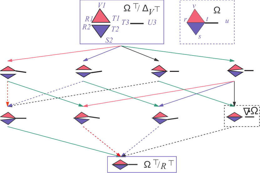
Figure 5.2: The decomposition lattice (See also Example 4.4.2) for the complex $\Omega$.

In Figure 5.2 we present an example of a decomposition lattice. This lattice is isomorphic to the the lattice of Figure 4.4. The reader must understand that these two figures actually contains two different lattices. In Figure 4.4, in the previous chapter, the top element was a quotient of $\Omega$ and in this first example we have chosen for $\Omega$ a complex made up of three connected components, i.e. two triangles and one edge. In Figure5.2 we take for $\Omega$ the complex made up of one connected component, i.e. the two triangles and the edge are stitched together. Then, at the top, in this figure, we have (a quotient of) $\Omega^{\top}$ that is, again, a complex made up of three connected components, two triangles and one edge.

It is easy to prove that the decomposition lattice is actually the lattice of all and alone the decompositions. This is expressed formally by the following two properties.

Property 5.4.1.

All quotients in the decomposition lattice are decompositions.

Proof 5.4.2.

Indeed, for a given element in the decomposition lattice $\Omega^{\prime}=\Omega^{\top}/{\approx}$ we have $\Delta_{V^{\top}}\leq{\approx}\leq R^{\top}$. Thus we always find two abstract simplicial maps one from $\Omega^{\top}/\Delta_{V^{\top}}$ to $\Omega^{\prime}$ and the other from $\Omega^{\prime}$ to $\Omega^{\top}/{R_{\top}}$ (see Properties 4.3.1 and 3.3.2). Since there is a dimension preserving bijection between top simplices in $\Omega^{\top}/\Delta_{V^{\top}}$ and $\Omega^{\top}/{R_{\top}}$ there must be a dimension preserving abstract simplicial map from $\Omega^{\prime}$ to $\Omega^{\top}/{R_{\top}}$. This will induce a bijection between top simplices in $\Omega^{\prime}$ and $\Omega^{\top}/{R_{\top}}$. By Definition 5.2.1 this proves that $\Omega^{\prime}$ is a decomposition of $\Omega^{\top}/{R_{\top}}$.

In general there is a dimension preserving abstract simplicial map between any ordered pair of decompositions in the decomposition lattice (by ordered pair we mean two decompositions such that $\Omega^{\top}/{\approx_{1}}\prec\Omega^{\top}/{\approx_{2}}$).

In the following we will study decompositions by studying the properties of the decomposition lattice. This is perfectly legal since all decompositions are in the decomposition lattice up to isomorphism. This is stated by the following property.

Property 5.4.2.

Each decomposition has an isomorphic copy in the decomposition lattice.

Proof 5.4.3.

$$\begin{CD}\Omega^{\prime}\cong(\Omega^{\prime})^{\top}/(R^{\prime})^{\top}@>{f}>{}>\Omega\cong\Omega^{\top}/R^{\top}\\ @A{(R^{\prime})^{\top}}A{h^{\prime}}A\\ (\Omega^{\prime})^{\top}@<{i}<{}<\Omega^{\top}\end{CD}$$

Let $\Omega^{\prime}$ be a decomposition for $\Omega$. Being $\Omega^{\prime}$ a decomposition there must be a dimension preserving abstract simplicial map $f$ from $\Omega^{\prime}$ to $\Omega\cong\Omega^{\top}/R^{\top}$. The situation of this proof is summarized in the communtative diagram above. This abstract simplicial map $f$ must be also a bijection between top simplices in $\Omega$ and $\Omega^{\prime}$. Hence, there must be a dimension preserving bijection between top simplices in the totally exploded versions of $\Omega$ and in the totally exploded version of $\Omega^{\prime}$. Therefore there must be an isomorphism between these two totally exploded versions. Let us denote with $i$ this isomorphism between $(\Omega^{\prime})^{\top}$ and $\Omega^{\top}$. By Property 5.3.1 there will be an equivalence $(R^{\prime})^{\top}$ and an associated abstract simplicial map $h^{\prime}$ from $(\Omega^{\prime})^{\top}$ to $\Omega^{\prime}\cong(\Omega^{\prime})^{\top}/(R^{\prime})^{\top}$. Similarly we introduce the abstract simplicial map  $h$ and equivalence $R^{\top}$ in the commutative diagram above. If we compose this isomorphism with the abstract simplicial map $h^{\prime}$ we obtain a dimension preserving abstract simplicial map $g$ from $\Omega^{\top}$ to $\Omega^{\prime}$ therefore $\Omega^{\prime}\prec\Omega^{\top}$. Hence, by Property 4.2.1 Part 4. $\Omega^{\top}/R_{g}\cong\Omega^{\prime}$ being $R_{g}$ the equivalence associated with $g$. This proves that $\Omega^{\top}/R_{g}$ is an element of the quotient lattice. We have to show that is in the decomposition lattice. We have $\Omega^{\top}/R^{\top}\cong\Omega\prec\Omega^{\prime}\cong\Omega^{\top}/R_{g}$. Thus $R_{g}\leq R^{\top}$ and therefore $\Omega^{\top}/R_{g}$ is an element of the decomposition lattice and this complexes the proof.

Hence in the following we will restrict our attention to the decomposition lattice and assume that all equivalences we consider are within $[{\Delta_{V^{\top}}},R_{\top}]$.

5.5 Equating Simplices

The elements in the decomposition lattice of a complex $\Omega$ are generated by stitching together vertices from the totally exploded decomposition of $\Omega$. Vertices that are glued together must not belong to the same top simplex. Thus, the decomposition lattice must be anti-isomorphic to the poset of partitions of vertices in the totally exploded decomposition of $\Omega$. In the partition $V^{\top}/{R_{\top}}$ (i.e. the partition of $V^{\top}$ induced by $R_{\top}$) there will be a block $\pi_{w}$ for each vertex $w\in V$. The block $\pi_{w}$ will be the subsets of $V^{\top}$ given by $\{w_{\theta}|\theta\in star({w},{\Omega})\cap\Theta\}$. Directly from the definition of pasting and from properties of the partition lattice $\Pi_{n}$ we have that:

Property 5.5.1 (Structure of the Decomposition Lattice).

1. Each element of the decomposition lattice is a complex given by the nerve of a refinement of the covering $\{R_{[v]}|[v]\in(V^{\top}/{R_{\top}})\}$;

2. the poset of coverings that generate the decomposition lattice, ordered by the refinement relation, is isomorphic with the sublattice $[V^{\top}/R_{\top},{V^{\top}/{\Delta^{V^{\top}}}}]$ of the partitions of $V^{\top}$;

3. in particular we pass from the immediate superior $V^{\top}/\approx_{1}$ to its immediate inferior $V^{\top}/\approx_{2}$ in $[V^{\top}/R_{\top},{V^{\top}/{\Delta^{V^{\top}}}}]$ by uniting together two blocks in $V^{\top}/\approx_{1}$.

By collapsing several pairs of vertices we can equate simplices that are distinct in the totally exploded version of $\Omega$. Let be $\approx\in[{\Delta_{V^{\top}}},R_{\top}]$ an equivalence on the Vertices of $\Omega^{\top}$ and let $\Omega^{\prime}$ be a decomposition in the decomposition lattice. If two distinct simplices $\gamma^{\prime}_{1}$ and $\gamma^{\prime}_{2}$ in $\Omega^{\prime}$ have a common pasted simplex via $\approx$ (i.e. $\gamma^{\prime}_{1}/{\approx}=\gamma=\gamma^{\prime}_{2}/{\approx}$) we will say that $\gamma^{\prime}_{1}$ and $\gamma^{\prime}_{2}$ are equating simplices for $\approx$. In this situation we will say and that $\gamma$ is a splitting simplex that splits into $\gamma^{\prime}_{1}$ and $\gamma^{\prime}_{2}$ when undoing $\approx$. We will say that $\gamma^{\prime}_{1}$ and $\gamma^{\prime}_{2}$ are two simplex copies for $\gamma$ under $\approx$. Note that, by hypothesis, $\Omega^{\prime}/{\approx}$ is still a decomposition. We note that all the non-common faces of the simplex copies (i.e. faces in $(\cup_{i}{\partial\gamma^{\prime}_{i}})-\cap_{i}{\partial\gamma^{\prime}_{i}}$) must be equating simplices for $\approx$.

We will say that a simplex copy $\gamma^{\prime}$ is a manifold equating simplex (resp. non manifold equating simplex) w.r.t. $\approx$ if the corresponding splitting simplex (i.e. $\gamma^{\prime}/{\approx}$) is a manifold (resp. non manifold) simplex.

If an equating simplex $\gamma^{\prime}\in\Omega^{\prime}$, for an equivalence $\approx$, is not a face of another equating simplex we will call $\gamma^{\prime}$ a top equating simplex for $\approx$. Not all the simplex copies of a certain simplex need to be a top equating simplex if one is. Whenever the simplex $\gamma$ is a vertex we will talk about vertex copies and splitting vertex

Chapter 6 Simplex Gluing instructions

6.1 Introduction

In the previous chapter we have studied the lattice of decomposition of a complex $\Omega$. We have seen that this is anti-isomorphic to a closed interval sublattice of the partition lattice. On top of the decomposition lattice we have the totally exploded version $\Omega^{\top}$ of $\Omega$ and we can walk on the decomposition lattice adding equations whose basic effect is to glue together two vertexes of $\Omega^{\top}$. In this section we take a different look at the decomposition lattice. We imagine that we do not have the option to glue single pairs of vertexes each time but we are forced to glue together two top simplexes $\theta^{\top}_{1}$ and $\theta^{\top}_{2}$ gluing together all vertexes they have in common in $\Omega$. We will call this move a simplex gluing instruction (or a gluing instruction for short). Next, in Section 6.4 we will show that gluing instructions define another lattice that is a proper subset of the decomposition lattice. This will complete a three level hierarchy of lattices that we devised to study the decomposition complex.

In this hierarchy, at the lowliest level, we have the lattice of quotients of $\Omega^{\top}$. This quotient lattice spans between the totally exploded decomposition of $\Omega$ and the single vertex resulting from the total collapse of $\Omega$ into a point. The lattice of quotients of $\Omega^{\top}$ offers the finest granularity and the maximum extension providing a representative for all possible modifications of $\Omega$. We believe that several problems in computer graphics can be modeled within the framework provided by this lattice. For instance the Vertex Tree in [82] can be described easily as an implementation of the closed interval $[\Omega^{\top}/(V^{\top}\times V^{\top}),\Omega^{\top}/R^{\top}]$ in the lattice of quotients of $\Omega^{\top}$.

Then we introduced another lattice is more specific for the decomposition problem. Indeed, in the previous chapter we have introduced the decomposition lattice as a closed interval within the lattice of quotient of $\Omega$. In this section, we will introduce the lattice of decomposition generated by sets of gluing instructions. This latter is a sublattice of the decomposition  lattice and represents an abstraction on it. This abstraction is central in the development of this thesis, In fact, Chapter 7, will be devoted to the study of the topological properties of elements in this lattice. In particular we will detail topological properties that are relevant for the decomposition problem. In Chapter 8, in particular in Lemma 8.2.1, we will prove that this lattice actually represents the right abstraction to master the decomposition problem and thus we build, in this lattice, our definition of standard decomposition.

6.2 Simplex Gluing instructions

We introduce gluing instructions to have an handy way to denote the set of stitching equations needed to completely stitch together top simplexes $\theta_{1}$ and $\theta_{2}$. To understand what we mean by ”completely stitch together” we first recall that there is a bijection between top simplexes in a complex $\Omega$ and top simplexes in any decomposition of the complex $\Omega$. Let us consider a pair of top simplexes $\theta_{1}$ and $\theta_{2}$ in $\Omega$ incident at the non-empty simplex $\gamma$ (i.e. $\gamma=\theta_{1}\cap\theta_{2}$). We might find that, in a decomposition $\Omega^{\top}/{\approx}$, the corresponding two top simplexes $\theta_{1}^{\top}/{\approx}$ and $\theta_{2}^{\top}/{\approx}$ might share a simplex $\gamma^{\prime}={\theta_{1}^{\top}/{\approx}}\cap{\theta_{2}^{\top}/{\approx}}$ whose dimension is smaller than $\mbox{\rm dim}{(\gamma)}$. For instance, let be $\theta_{1}$ and $\theta_{2}$ two tetrahedra in a $3$-complex $\Omega$ and let $\gamma$ be their common simplex (i.e. $\gamma=\theta_{1}\cap\theta_{2}$). For instance $\gamma$ could be a triangle. Now there are decomposition $\Omega^{\top}/{\approx}$ where top tetrahedra $\theta_{1}^{\top}/{\approx}$ and $\theta_{2}^{\top}/{\approx}$ do not share a full triangle but simply an edge or a tip. In this case we will say that $\theta_{1}$ and $\theta_{2}$ (or $\theta_{1}^{\top}/{\approx}$ and $\theta_{2}^{\top}/{\approx}$) do not completely stitch together. On the other hand, we will say that, in the decomposition $\Omega^{\top}/{\approx}$, top simplexes $\theta_{1}$ and $\theta_{2}$ completely stitch together if and only if top simplexes $\theta_{1}^{\top}/{\approx}$ and $\theta_{2}^{\top}/{\approx}$ intersect at a simplex with the same dimension of $\gamma=\theta_{1}\cap\theta_{2}$. In the case of our example of the two tetrahedra sharing a triangle in $\Omega$ we will say that they completely stitch together in all decompositions $\Omega^{\top}/{\approx}$ where they share a triangle.

A simplex gluing instruction (or simply a gluing instruction for short) is a pair, $g=\{\theta_{1},\theta_{2}\}\subset\Theta$, of top simplexes in the set of top simplexes $\Theta$ of $\Omega$, The gluing instruction $g$ will be usually written as $\theta_{1}\leftrightarrow\theta_{2}$ (or $\theta_{2}\leftrightarrow\theta_{1}$). If $\gamma$ is the common simplex, i.e. $\gamma=\theta_{1}\cap\theta_{2}$, to highlight the role of the common simplex $\gamma$, we will use $g_{\gamma}$, instead of plain $g$, to denote the gluing instruction made up of a pair of top simplexes that intersect at $\gamma=\theta_{1}\cap\theta_{2}$.

Simplex gluing instructions are synctatic objects that denotes an equivalence on vertexes of $\Omega^{\top}$. With this idea in mind we define the set of equations associated with the gluing instruction $\theta_{1}\leftrightarrow\theta_{2}$. as the set $\{v_{\{\theta_{1}\}}\approx v_{\{\theta_{2}\}}|v\in\theta_{1}\cap\theta_{2}\}$. We will say that ${\theta_{1}\leftrightarrow\theta_{2}}$ denotes the equivalence defined by this set of stitching equations. Whenever we need to put more emphasis on the denoted object we will use the symbol $\approx^{\theta_{1}\leftrightarrow\theta_{2}}$ to talk about the denoted equivalence. In all other cases, when this is not ambiguous, we will use the notation ${\theta_{1}\leftrightarrow\theta_{2}}$ to denote: the simplex gluing instruction, the associated set of stitching equations and the equivalence $\approx^{\theta_{1}\leftrightarrow\theta_{2}}$.

We will say that the equivalence ${\approx}$ satisfies instruction ${\theta_{1}\leftrightarrow\theta_{2}}$ whenever the equivalence $\approx^{\theta_{1}\leftrightarrow\theta_{2}}$, is contained in the equivalence ${\approx}$ (i.e. $\approx^{\theta_{1}\leftrightarrow\theta_{2}}\subset{\approx}$)).

Given a gluing instruction $\theta_{1}\leftrightarrow\theta_{2}$ we will define the gluing instruction order as $\dim{(\theta_{1}\cap\theta_{2})}$. Note that the order of $\theta_{1}\leftrightarrow\theta_{2}$ is one unit less the number of stitching equations associated with the gluing instruction.

Note that we do not ask the two top simplexes $\theta_{1}$ and $\theta_{2}$ to be incident. However, if the two simplexes $\theta_{1}$ and $\theta_{2}$ are disjoint, we have that the associated set of equations is empty. In this case we will call the gluing instruction $\theta_{1}\leftrightarrow\theta_{2}$ empty or void. By convention we assign order $-1$ to empty instructions.

6.3 Sets of gluing instructions

Given a set ${\mathcal{E}}=\{g_{i}\}$ of gluing instructions we associate a set of stitching equations to ${\mathcal{E}}$ by taking all the stitching equations associated with each ${g_{i}}$. We will say that ${\mathcal{E}}$ is associated (or denotes) this set of stitching equations. We will use the symbol $\approx^{\mathcal{E}}$ (or ${\mathcal{E}}$ as a shortcut) to denote the equivalence induced by the set of stitching equations associated with ${\mathcal{E}}$. We extend this notation to the empty set by taking the identity relation for $\approx^{\emptyset}$. If $\approx^{\mathcal{E}}\subset{\approx}$ we will say that equivalence $\approx$ satisfies the set of gluing instructions ${\mathcal{E}}$. This happens if and only if $\approx$ satisfy all stitching equations in ${\mathcal{E}}$. Thus we will write $\Omega^{\top}/{\mathcal{E}}$ and $\gamma/{\mathcal{E}}$ to denote both $\Omega^{\top}/{\approx^{\mathcal{E}}}$ and $\gamma/{\approx^{\mathcal{E}}}$. In particular we will say that the set of gluing instructions ${\mathcal{E}}$ generates the quotient $\Omega^{\top}/{{\mathcal{E}}}$. Furthermore, according to Definition 4.3.5 it is perfectly legal to write $\Omega^{\prime}/{\mathcal{E}}$ for a decomposition $\Omega^{\prime}=\Omega^{\top}/{\mathcal{E}}^{\prime}$. In fact this unfolds to $\Omega^{\prime}/{\mathcal{E}}=(\Omega^{\top}/{\mathcal{E}}^{\prime})/{\mathcal{E}}=(\Omega^{\top}/{\approx^{{\mathcal{E}}^{\prime}}})/{\approx^{\mathcal{E}}}$ and Definition 4.3.5 this becomes $\Omega^{\top}/({\approx^{{\mathcal{E}}^{\prime}}}+{\approx^{\mathcal{E}}})$

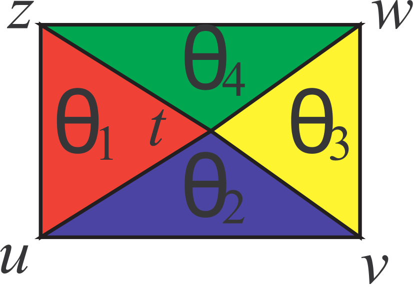
(a)

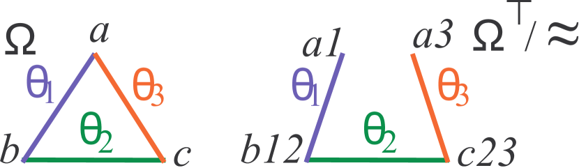
(b)

Figure 6.1: An example of a complex with redundant gluing instructions (a) and non transitivity for $\leftrightarrow$ (b)

Example 6.3.1.

The $\Omega/{\mathcal{E}}$ notation suggest an easy similarity between quotients of the form $\Omega/E$, defined by a set of stitching equations $E$, and quotients of the form ${\Omega/{\mathcal{E}}}$, defined by a set of gluing instructions ${\mathcal{E}}$. Undoubtly strong relation between these two families exists. However, some care must be taken in extending concepts for sets of stitching equations to sets of gluing instructions. A first flaw is in the concept of independent set of equations. There are quite obvious examples of non redundant sets of gluing instruction whose associated set of stitching equations is not independent.

See for instance the complex of Figure 6.1a. Consider the set of gluing instructions ${\mathcal{E}}=\{{\theta_{1}\leftrightarrow\theta_{2}},{\theta_{2}\leftrightarrow\theta_{3}},{\theta_{3}\leftrightarrow\theta_{4}},{\theta_{4}\leftrightarrow\theta_{1}}\}$. The corresponding pairs of stitching equations, a pair for each gluing instructions, above are: $\{{u1\approx u2},{t1\approx t2}\}$, $\{{v2\approx v3},{t2\approx t3}\}$, $\{{w3\approx w4},{t3\approx t4}\}$ and $\{{z4\approx z1},{t4\approx t1}\}$. The set of stitching equations ${\mathcal{E}}$ is a set of non redundant instructions. No instruction in the set ${\mathcal{E}}$ can be deleted without decomposing the generated complex. For instance we cannot delete gluing instruction  $\theta_{4}\leftrightarrow\theta_{1}$. In fact, in this case, we have that equation ${z4\approx z1}$ is not satisfied by the equivalence induced by the first three gluing instruction. However, the set of eight equations associated with ${\mathcal{E}}$ is not a set of independent stitching equations. In fact ${t4\approx t1}$ is already satisfied by the equivalence induced by the six stitching equations in the first three pairs corresponding to the set of gluing instructions:. $\{{\theta_{1}\leftrightarrow\theta_{2}},{\theta_{2}\leftrightarrow\theta_{3}},{\theta_{3}\leftrightarrow\theta_{4}}\}$.

6.4 The lattice of quotients modulo gluing instructions

In this section we will show that sets of gluing instructions define another lattice that is a proper subset of the decomposition lattice. This will complete the three level hierarchy of lattices that we devised to study the decomposition complex.

We will see in this section that the lattice of decomposition generated by sets of gluing instruction is a point lattice that is a proper subset of the decomposition lattice. In fact, in some cases, not all elements of the decomposition lattice can be generated by sets of gluing instruction.

We will denote with ${\mathcal{E}}^{\star}$ the set of all non empty gluing instructions satisfied by $\approx^{\mathcal{E}}$. Directly from the definition we have that $\approx^{{\mathcal{E}}^{\star}}=\approx^{{\mathcal{E}}}$ and $\Omega^{\top}/{\mathcal{E}}^{\star}=\Omega^{\top}/{\mathcal{E}}$. If a set of gluing instructions is such that ${\mathcal{E}}^{\star}={\mathcal{E}}$ we will say that set ${\mathcal{E}}$ is closed. Note that in a closed set of gluing instructions the symbol ${\theta_{1}\leftrightarrow\theta_{2}}$ do not denotes a transitive relation. Indeed we may have complexes $\Omega$ with some decomposition $\Omega^{\top}/{\approx}$ for which we have that $\approx$ satisfy both $\theta_{1}\leftrightarrow\theta_{2}$ and $\theta_{2}\leftrightarrow\theta_{3}$ and yet we might find that $\approx$ do not satisfies $\theta_{1}\leftrightarrow\theta_{3}$. This might happens even if equivalence $\approx$ is defined by a closed set of gluing instructions.

Example 6.4.1.

The simplest example in this sense is given by the $1$-complex $\Omega$ of Figure 6.1b. Complex $\Omega$ is given by the three segments $\theta_{1}=ab$, $\theta_{2}=bc$ and $\theta_{3}=ca$. Consider now the decomposition $\Omega^{\top}/{\approx}$ where edges $\theta_{1}$ and $\theta_{3}$ do not stitch together at $a$. We have that equivalence $\approx$ satisfy gluing instructions $\theta_{1}\leftrightarrow\theta_{2}$ and $\theta_{2}\leftrightarrow\theta_{3}$. However equivalence $\approx$ do not satisfy $a1\approx a3$ and therefore do not satisfy gluing instructions  $\theta_{1}\leftrightarrow\theta_{3}$. Note that the set of stitching equations associated with the set of two gluing instructions. ${\mathcal{E}}=\{\theta_{1}\leftrightarrow\theta_{2},\theta_{2}\leftrightarrow\theta_{3}\}$ is exactly made up by the two stitching equations $b1\approx b2$ and $c2\approx c3$. These two equations defines the equivalence $\approx$. No other gluing instruction is satisfied by $\approx{=}\approx^{\mathcal{E}}$ and therefore the pair of gluing instructions  ${\mathcal{E}}$ is closed.

Closed sets of gluing instructions form a poset that is ordered by set inclusion. To prove this we note that the intersection of two closed sets of gluing instructions is still a closed set of gluing instructions. Thus the set of closed gluing instructions has a closure property (see Appendix A  Section A.4). It is easy to see why the set ${{\mathcal{E}}_{1}}^{\star}\cap{{\mathcal{E}}_{2}}^{\star}$ is closed. If we need to add a gluing instruction to close it this must be both in ${{\mathcal{E}}_{1}}^{\star}$ and in ${{\mathcal{E}}_{2}}^{\star}$ since they are both closed. So it must be in the intersection. In general a set with the closure property is a complete lattice ordered by set inclusion. Whenever the closure property holds it can be proven that lattice operations are ${{\mathcal{E}}_{1}}^{\star}\cap{{\mathcal{E}}_{2}}^{\star}$ and ${({{\mathcal{E}}_{1}}^{\star}\cup{{\mathcal{E}}_{2}}^{\star})}^{\star}$ giving, respectively, the g.l.b. and the l.u.b. of ${{\mathcal{E}}_{1}}^{\star}$ and ${{\mathcal{E}}_{2}}^{\star}$. Thus, we have that closed sets of gluing instructions form a lattice. By definition, this lattice is a point lattice (see Appendix A Definition A.4.2). In fact all elements in this lattice are generated joining (i.e. summing) a basic set of elements called points or atoms. The points for this lattice are singletons of the form $\{\theta_{1}\leftrightarrow\theta_{2}\}$ containing a single gluing instruction.

The mapping that sends each set of gluing instructions ${\mathcal{E}}$ into the decomposition  $\Omega^{\top}/{\mathcal{E}}$, although not injective in general, becomes injective if restricted to closed sets of gluing instructions. This mapping sends the lattice of closed sets of gluing instructions into the set of decomposition  generated by gluing instructions. It is easy two see that this mapping is antitone (i.e. it reverses ordering, see Appendix A Section A.2). Thus the set of decompositions generated by gluing instructions must be a lattice anti-isomorphic to the lattice of closed sets of gluing instructions. Thus the set of decompositions of the form $\Omega^{\top}/{\mathcal{E}}$ is a lattice. Unfortunately this lattice, in general, is not a sublattice of the decomposition lattice. Indeed it is quite easy to build two closed sets of gluing instructions ${{\mathcal{E}}_{1}}^{\star}$ and ${{\mathcal{E}}_{2}}^{\star}$ such that the decomposition $\Omega^{\top}/({\approx^{{{\mathcal{E}}_{1}}^{\star}}}\cdot\approx^{{{{\mathcal{E}}_{2}}}^{\star}})$ is not the l.u.b. of $\Omega^{\top}/{{\mathcal{E}}_{1}}^{\star}$ and $\Omega^{\top}/{{\mathcal{E}}_{2}}^{\star}$ given by $\Omega^{\top}/({{{\mathcal{E}}_{1}}^{\star}}\cup{{{\mathcal{E}}_{2}}}^{\star})$. Therefore $\Omega^{\top}/({\approx^{{{\mathcal{E}}_{1}}^{\star}}}\cdot\approx^{{{{\mathcal{E}}_{2}}}^{\star}})$ is not a decomposition of the form $\Omega^{\top}/{\mathcal{E}}$.

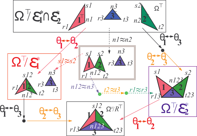
Figure 6.2: A lattice where ${\Omega^{\top}/(\approx^{{\mathcal{E}}_{1}}\cdot{\approx^{{\mathcal{E}}_{2}}})}$ is not a decomposition generated by a set of gluing instructions

Example 6.4.2.

Consider for instance the lattice in Figure 6.2. We have two disjoint sets of gluing instructions ${{\mathcal{E}}_{1}}^{\star}=\{\theta_{1}\leftrightarrow\theta_{2}\}$ and ${{\mathcal{E}}_{2}}^{\star}=\{\theta_{1}\leftrightarrow\theta_{3},\theta_{2}\leftrightarrow\theta_{3}\}$ that generates the two decompositions $\Omega^{\top}/{{\mathcal{E}}_{1}}^{\star}$ and $\Omega^{\top}/{{\mathcal{E}}_{2}}^{\star}$ It is easy to verify that the intersection of the corresponding equivalences $\approx^{{{\mathcal{E}}_{1}}^{\star}}$ and $\approx^{{{\mathcal{E}}_{2}}^{\star}}$ is not empty. This intersection is the equivalence defined by equation $n1\approx n2$.

We have that the decomposition $\Omega^{\top}/{\{{n1\approx n2}\}}$ is the least upper bound in the decomposition lattice for the pair of complexes $\Omega^{\top}/{{\mathcal{E}}_{1}}^{\star}$ and $\Omega^{\top}/{{\mathcal{E}}_{2}}^{\star}$. Similarly equivalence $\{{n1\approx n2}\}$ is the greatest lower bound ${{\approx^{{{\mathcal{E}}_{1}}^{\star}}}\cdot{\approx^{{{\mathcal{E}}_{2}}^{\star}}}}$. Equivalence ${\{{n1\approx n2}\}}$ is not an equivalence of the form ${\approx^{{\mathcal{E}}}}$. Indeed there is not a set of gluing instructions ${\mathcal{E}}$ such that ${\approx^{{\mathcal{E}}}}={\{{n1\approx n2}\}}$.

Furthermore, equivalence generated by sets of gluing instructionform a lattice that is not semimodular. This can be seen in the example of Figure 6.3

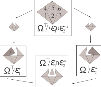
Figure 6.3: A lattice where the two elements ${\Omega^{\top}/{{\mathcal{E}}_{1}}^{\star}}$ and ${\Omega^{\top}/{{\mathcal{E}}_{2}}^{\star}}$ are both immediate superior to $\Omega^{\top}/{{{{\mathcal{E}}_{1}}}^{\star}\cap{{{\mathcal{E}}_{2}}^{\star}}}$ and there is not a a common immediate superior for ${\Omega^{\top}/{{\mathcal{E}}_{1}}^{\star}}$ and ${\Omega^{\top}/{{\mathcal{E}}_{2}}^{\star}}$

Example 6.4.3.

We recall that a lattice is semimodular if and only if  whenever two elements has a common immediate inferior they also have a common immediate superior (see Appendix A Definition A.4.3). In the lattice of Figure 6.3 we have

$${{{{\mathcal{E}}_{1}}^{\star}\cap{{\mathcal{E}}_{2}}^{\star}}=\{{\theta_{4}\leftrightarrow\theta_{1}},{\theta_{1}\leftrightarrow\theta_{2}},{\theta_{2}\leftrightarrow\theta_{3}},{\theta_{3}\leftrightarrow\theta_{6}}\}}$$

. Then adding ${\theta_{4}\leftrightarrow\theta_{5}}$ (i.e. glue the two gray triangles on the left) we get ${{\mathcal{E}}^{\star}_{1}}$ Adding ${\theta_{5}\leftrightarrow\theta_{6}}$ (i.e. glue the two gray triangles on the right) we get ${{\mathcal{E}}_{2}}^{\star}$. The set ${{{\mathcal{E}}_{1}}^{\star}\cap{{\mathcal{E}}_{2}}^{\star}}^{\star}$ is the l.u.b. for the pair ${{\mathcal{E}}_{1}}^{\star}$ and ${{\mathcal{E}}_{2}}^{\star}$. Unfortunately this element is not the immediate superior for neither ${{\mathcal{E}}_{1}}^{\star}$ nor ${{\mathcal{E}}_{2}}^{\star}$. This is due to the presence of the two small unframed complexes in Figure 6.3. This proves that the proposed lattice is not semimodular.

The lack of semimodularity impair the possibility of having a grade for decomposition based on the size of the set of gluing instructions necessary to build them.

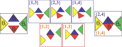
Figure 6.4: Two ways of forming the complex on the right with four (upper path) and three (lower path) gluing instructions. In both paths each gluing instruction always add independent stitching equations

Example 6.4.4.

Consider the situation of Figure 6.4. We can go from the complex on the extreme left to the complex on the extreme right following two paths. The upper path is made up of four hops. Collecting gluing instructions that labels each hop we get a set of four gluing instructions. In each frame we report the gluing instruction that is necessary to reach the complex at the end of each hop. We use the shortcut $\{i,j\}$ for the instruction $\theta_{i}\leftrightarrow\theta_{j}$. With this convention we collect, along the upper path, the four gluing instructions: ${\theta_{1}\leftrightarrow\theta_{3}}$, ${\theta_{2}\leftrightarrow\theta_{3}}$, ${\theta_{1}\leftrightarrow\theta_{4}}$ and ${\theta_{2}\leftrightarrow\theta_{4}}$. Similarly, lower in Figure 6.4, we have a path made up of just three hops. Along this path we collect just three instructions: ${\theta_{1}\leftrightarrow\theta_{2}}$, ${\theta_{1}\leftrightarrow\theta_{3}}$ and ${\theta_{1}\leftrightarrow\theta_{4}}$. Both sets of gluing instructions are associated with a set of four independent stitching equations. Indeed the complex on the extreme left is of grade four in the decomposition lattice.

This example shows that a grade based on the number of gluing instruction is not possible and this is a major consequence of the lack of semimodularity.

We close this section with a very simple example that shows the subset of the lattice of decomposition in Figure 4.4 obtained taking complexes generated by gluing instructions.

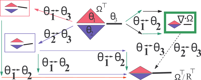
Figure 6.5: A reduced  lattice out of lattice of Figure 4.4

Figure 6.5 is a reduced version of Figure 4.4 obtained by deleting decomposition that are not of the form $\Omega^{\top}/{\mathcal{E}}$. Arrows are reported with the colors they have in Figure 4.4. Colored arrows denote stitching equations that’s why path for a gluing instruction corresponds to more than one arrow. Groups of colored arrows are labeled with the gluing instruction that transforms the complex at the origin of the arrow into the complex at the tip of the arrow. So, for instance, let us start at complex with the thick frame. This is $\Omega^{\top}/{\{\theta_{1}\leftrightarrow\theta_{2}\}}$. By following the black dashed line we must add ${\theta_{1}\leftrightarrow\theta_{3}}$ or ${\theta_{2}\leftrightarrow\theta_{3}}$ and reach (the isomorphic copy of) $\Omega$ at the bottom. The bottom is generated either by the set $\{\theta_{1}\leftrightarrow\theta_{2},\theta_{1}\leftrightarrow\theta_{3}\}$ or by the set $\{\theta_{1}\leftrightarrow\theta_{2},\theta_{2}\leftrightarrow\theta_{3}\}$.

Chapter 7 Simplex Gluing instructions and Topological properties

7.1 Introduction

Given a decomposition generated by a set of gluing instruction  ${\mathcal{E}}$, it is possible to connect the topological properties of $\Omega^{\top}/{{\mathcal{E}}}$ with properties of the set of gluing instruction ${\mathcal{E}}$. Indeed we will develop an analysis of complexes generated by a set of gluing instructions ${\mathcal{E}}$. This analysis gives some topological properties for the decomposition $\Omega^{\top}/{{\mathcal{E}}}$ on the ground of properties of gluing instructions in ${\mathcal{E}}$.

Note that some of the properties for ${\mathcal{E}}$ are defined considering the relation between instructions in the set ${\mathcal{E}}$ and the complex $\Omega$. Properties for the set of instructions ${\mathcal{E}}$ do not refer to the generated complex $\Omega^{\top}/{{\mathcal{E}}}$ and note that, in general, $\Omega^{\top}/{{\mathcal{E}}}$ is not $\Omega^{\top}/{R_{\top}\cong\Omega}$. This formulation is due since we are interested in the set of all complexes of the form $\Omega^{\top}/{{\mathcal{E}}}$ that are decompositions of $\Omega$.

However, we note that topologic properties of complex $\Omega$ can be discussed by considering the set of gluing instructions that builds $\Omega$, (i.e. the set of gluing instructions ${\mathcal{E}}$ such that $\Omega^{\top}/{{\mathcal{E}}}=\Omega^{\top}/{R_{\top}\cong\Omega}$. Thus, results in this chapter applies to all modeling approaches that builds a simplicial complex gluing together top simplices using operators that can be modeled by simplex gluing instructions.

In the following we will derive relations between the structure of a set of gluing instructions ${\mathcal{E}}$ and the topological properties of the complex $\Omega^{\top}/{{\mathcal{E}}}$. We will first consider the usual topological properties defined in Chapter 3 such as regularity, connectivity, pseudomanifoldness and manifoldness. Next we will consider Quasi-manifold [80] and a superset of quasi-manifoldwe called initial-quasi-manifold. The latter being particularly relevant for the forthcoming study of decompositions.

7.2 Regularity, Connectivity Pseudomanifoldness

In this section we give a characterization of topological properties for $\Omega^{\top}/{\mathcal{E}}$ in term of property for the set of gluing instructions ${\mathcal{E}}$.

7.2.1 Regularity

We start with regularity as defined in Section 3.2.4. We will say that a gluing instruction ${\theta_{1}\leftrightarrow\theta_{2}}$ is regular if $\mbox{\rm dim}{(\theta_{1})}=\mbox{\rm dim}{(\theta_{2})}$. For a regular instruction ${\theta_{1}\leftrightarrow\theta_{2}}$ we define the dimension of the instruction as the dimension $\mbox{\rm dim}{(\theta_{1})}=\mbox{\rm dim}{(\theta_{2})}$. Note that the dimension of a regular instruction must not be confused with the order of an instruction given by $\mbox{\rm dim}{(\theta_{1}\cap\theta_{2})}$.

It is easy to show that we can generate a complex whose connected components are regular if and only if we use a set of regular gluing instructions.

Property 7.2.1.

The connected components of   $\Omega^{\top}/{\mathcal{E}}$ are regular if and only if all instructions in ${\mathcal{E}}$ are regular

Proof 7.2.1.

First let us prove that if $\Omega^{\top}/{\mathcal{E}}$ has regular connected components, then all instructions in ${\mathcal{E}}$ must be regular. If ${\theta_{1}\leftrightarrow\theta_{2}}$ is an instruction in ${\mathcal{E}}$ then the two top simplices $\theta^{\top}_{1}/{\mathcal{E}}$ and $\theta^{\top}_{2}/{\mathcal{E}}$ share some simplex in $\Omega^{\top}/{\mathcal{E}}$. Therefore the two top simplices $\theta^{\top}_{1}/{\mathcal{E}}$ and $\theta^{\top}_{2}/{\mathcal{E}}$ belongs to the same connected component. Since each connected component is regular we have $\mbox{\rm dim}{({\theta^{\top}_{1}/{\mathcal{E}}})}=\mbox{\rm dim}{({\theta^{\top}_{2}/{\mathcal{E}}})}$. It is easy to see that we have, for $i=1,2$, $\mbox{\rm dim}{({\theta^{\top}_{i}/{\mathcal{E}}})}=\mbox{\rm dim}{({\theta^{\top}_{i}})}=\mbox{\rm dim}{({\theta_{i}})}$. Thus $\mbox{\rm dim}{({\theta^{\top}_{1}/{\mathcal{E}}})}=\mbox{\rm dim}{({\theta^{\top}_{2}/{\mathcal{E}}})}$ gives $\mbox{\rm dim}{({\theta_{1}})}=\mbox{\rm dim}{({\theta_{2}})}$ This proves that instruction ${\theta_{1}\leftrightarrow\theta_{2}}$ must be regular.

Conversely let be ${\mathcal{E}}$ a set of regular gluing instructions. and let be $E$ the set of independent stitching equations in the set of stitching equations associated with ${\mathcal{E}}$. For each equation $v_{\theta_{1}}\approx v_{\theta_{2}}$ in $E$ we have that $\mbox{\rm dim}{(\theta_{1})}=\mbox{\rm dim}{(\theta_{2})}$. In this case we will say that equation $v_{\theta_{1}}\approx v_{\theta_{2}}$ has dimension $h=\mbox{\rm dim}{(\theta_{1})}=\mbox{\rm dim}{(\theta_{2})}$. We will prove that if stitching equations in $E$ has this property then the connected components of the generated complex $\Omega^{\top}/E$ are regular. In particular the connected components of dimension $h$ are given by $\Omega^{\top}_{h}/E_{h}$ where $\Omega^{\top}_{h}$ is the subcomplex of $\Omega^{\top}$ of all $h$-simplices and $E_{h}$ is the subset of equations of $E$ of dimension $h$. We will prove this by induction on the number $|E|$ of independent stitching equations.

For $|E|=0$ must be $E=\emptyset$ and $\Omega^{\top}/\emptyset\simeq\Omega^{\top}$. Obviously, connected components in $\Omega^{\top}$ are regular. In fact, in $\Omega^{\top}$, each top simplex is a connected component on its own.

Now, for $|E|>0$ let us consider $E^{\prime}=E-\{v_{\theta_{1}}\approx v_{\theta_{2}}\}$ By inductive hypothesis we have that $\Omega^{\top}/{E^{\prime}}$ has regular connected components. We have that, for $i=1,2$. $v_{\theta_{i}}/{E^{\prime}}\in{\theta^{\top}_{i}}/{E^{\prime}}$ and $\mbox{\rm dim}{(\theta^{\top}_{1}/{E^{\prime}})}=\mbox{\rm dim}{(\theta_{1})}=\mbox{\rm dim}{(\theta_{2})}=\mbox{\rm dim}{(\theta^{\top}_{2}/{E^{\prime}})}=h$. So, by inductive hypothesis, $v_{\theta_{1}}/{E^{\prime}}$ and $v_{\theta_{2}}/{E^{\prime}}$ belongs to two regular connected components of $\Omega^{\top}/{E^{\prime}}$ of the dimension $h$ within $\Omega^{\top}_{h}/E^{\prime}_{h}$. Now adding $v_{\theta_{1}}\approx v_{\theta_{2}}$ we map $\Omega^{\top}/{E^{\prime}}$ into $\Omega^{\top}/E$. and $v_{\theta_{1}}/{E^{\prime}}$ collapse with $v_{\theta_{2}}/{E^{\prime}}$. This possibly merges two regular connected components of dimension $h$. Therefore $\Omega^{\top}/E$ will have regular connected components, too.

The complex generated by a set of regular instructions ${\mathcal{E}}$ has regular connected components. From the proof of the previous property we have that all connected components of dimension $h$ are generated by the subset of regular instructions of dimension $h$. This is stated by the following property.

Property 7.2.2.

Let be ${\mathcal{E}}$ a set of regular gluing instructions for a $d$-complex $\Omega$. For all $0\leq h\leq d$ let be ${\mathcal{E}}_{h}$ the subset of instructions of dimension $h$ and let be $\Omega^{\top}_{h}$ the subcomplex of   $\Omega^{\top}$ containing all top simplices of   $\Omega^{\top}$ of dimension $h$. In this situation the set of connected components of dimension $h$ is the subcomplex of   ${\Omega^{\top}/{\mathcal{E}}}$ given by $\Omega^{\top}_{h}/{{\mathcal{E}}_{h}}$.

7.2.2 Connectivity

Another topological property that admits an easy characterization in term of gluing instructions is $h$-connectivity (see Section 3.2.3). It is easy to see that if ${\theta_{1}\leftrightarrow\theta_{2}}$ and ${\theta_{2}\leftrightarrow\theta_{3}}$ are two gluing instructions  in ${\mathcal{E}}$ then $\theta_{1}$ and $\theta_{3}$ are at least $k$-connected where $k$ is the minimum order between that of the two instructions. In general it can be proved that, if we apply a set ${\mathcal{E}}_{k}$ of gluing instructions of order smaller or equal than $k$, we obtain several sets of top simplices bundled in $k$-connected components. More precisely the following property holds:

Property 7.2.3.

Let be $\Omega$ a $d$-complex with top simplices in $\Theta$ and let ${\mathcal{E}}$ be a set of gluing instructions. For for any $k<d$ let ${\mathcal{E}}_{k}$ be the subset of gluing instructions in ${\mathcal{E}}$ of order smaller or equal to $k$. Let $R_{k}$ be the smallest equivalence on $\Theta^{\top}$ that contains the relation $\{(\theta^{\top}_{1},\theta^{\top}_{2})|{\theta_{1}\leftrightarrow\theta_{2}}\in{{\mathcal{E}}_{k}}\}$. In this situation each block in the partition of top simplices $\Theta^{\top}/R_{k}$ gives a set of top simplices $\Omega^{\top}/{\mathcal{E}}$ that are $k$-connected. If ${\mathcal{E}}$ is a closed set of gluing instructions then $\Theta^{\top}/R_{k}$ gives the partition of $\Theta^{\top}$ induced by the $k$-connected components of  $\Omega^{\top}/{\mathcal{E}}$.

Proof 7.2.2.

For each pair of top simplices $\theta^{\top}_{a}$ and $\theta^{\top}_{b}$ in a block of partition $\Theta^{\top}/R_{k}$ we can find a sequence $(\theta^{\top}_{i})_{i=0}^{n}$ of top simplices that describe a $k$-path in $\Omega^{\top}/{\mathcal{E}}$ (i.e. $(\theta^{\top}_{i}/{\mathcal{E}})_{i=0}^{n}$ ) between $\theta^{\top}_{a}/{\mathcal{E}}$ and $\theta^{\top}_{b}/{\mathcal{E}}$. Indeed, being $\theta^{\top}_{a}R_{k}\theta^{\top}_{b}$, we can select the $\theta^{\top}_{i}$ such that $\theta^{\top}_{a}=\theta^{\top}_{0}$, $\theta^{\top}_{n}=\theta^{\top}_{b}$ and such that $\theta^{\top}_{i}R_{k}\theta^{\top}_{i+1}$ (i.e. $\theta_{i}\leftrightarrow\theta_{i+1}$ is in ${\mathcal{E}}_{k}$). Thus, $\theta^{\top}_{i}/{\mathcal{E}}$ and $\theta^{\top}_{i+1}/{\mathcal{E}}$ share a $k$-face in $\Omega^{\top}/{\mathcal{E}}$. This proves that every block in $\Theta^{\top}/R_{k}$ is $k$-connected in $\Omega^{\top}/{\mathcal{E}}$.

Conversely if $\theta^{\top}_{a}/{\mathcal{E}}$ and $\theta^{\top}_{b}/{\mathcal{E}}$ are $k$-connected in $\Omega^{\top}/{\mathcal{E}}$ we can select a $k$-path . $(\theta^{\top}_{i}/{\mathcal{E}})$ made up of top simplices in between $\theta^{\top}_{a}/{\mathcal{E}}$ and $\theta^{\top}_{b}/{\mathcal{E}}$. Thus, $\theta^{\top}_{i}/{\mathcal{E}}$ and $\theta^{\top}_{i+1}/{\mathcal{E}}$ must share at least a $k$-face. Thus $\theta_{i}\leftrightarrow\theta_{i+1}$ must be a gluing instruction of order greater or equal to $k$ and must be satisfied by ${\mathcal{E}}$. Being the set ${\mathcal{E}}$ closed we must have that $\theta_{i}\leftrightarrow\theta_{i+1}$ is in ${\mathcal{E}}$ and thus $\theta^{\top}_{i}R_{k}\theta^{\top}_{i+1}$. Thus $\theta^{\top}_{a}$ and $\theta^{\top}_{b}$ must be in the same block of the partition $\Theta^{\top}/R_{k}$.

For a complex generated by a set of gluing instructions of order greater or equal to $h$ we have that $\Theta^{\top}/R_{k}$ do not change for all $k\leq h$. Thus, this complex must have connected components that are at least $h$-connected. However note that is easy to find examples of complexes generated by set of gluing instructions of order $0$ that have non trivial $1$-connected components. See for instance the upper path for the construction of the rightmost complex in Figure 6.4. This path contains the application of four gluing instructions of order $0$ (i.e. ${\theta_{1}\leftrightarrow\theta_{3}}$, ${\theta_{2}\leftrightarrow\theta_{3}}$, ${\theta_{1}\leftrightarrow\theta_{4}}$ and ${\theta_{2}\leftrightarrow\theta_{4}}$.) and yet the generated complex has non trivial $1$-connected components. This do not contrasts with the second part of Property 7.2.3 since this set of four gluing instructions of order $0$ is not a closed set of gluing instructions. On the other hand, if a complex is $h$-connected and is not $(h+1)$-connected, not necessarily it can be generated by a set of gluing instructions  of order lower than $h$. This is an obvious consequence of the fact that $h$-connectivity need to hold all across the complex.

Example 7.2.3.

Figure 7.1a, shows an obvious example of a $0$-connected complexes that is not $1$-connected and yet can only be generated by sets of gluing instructions that must contain the instruction  ${\theta_{1}\leftrightarrow\theta_{2}}$. This is an instruction of order $1$.

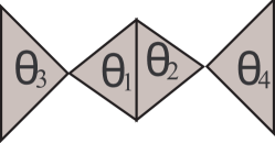
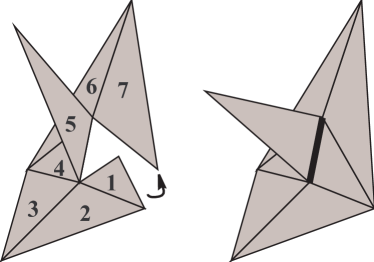
(a) (b)

Figure 7.1: An example (a) of a $0$-connected non $1$-connected complex that cannot be generated using only instructions of order $0$ (see Example 7.2.3). In (b) we have an example of a non-pseudomanifold complex generated by a non closed set set of pseudomanifold instructions (see Example 7.2.7)

7.2.3 Pseudomanifoldness

Next we analyze the relation between a set of instructions ${\mathcal{E}}$ and the pseudomanifoldness of the generated complex. A non void gluing instruction $\theta_{1}\leftrightarrow\theta_{2}$ will be called a manifold (resp. non manifold) instruction (w.r.t $\Omega$) iff $\theta_{1}\cap\theta_{2}$ is a manifold (resp. non manifold) simplex in $\Omega$. In the following, unless otherwise stated, we will assume that manifold and non-manifold instructions are referred to $\Omega$. Therefore we will simply say that an instruction $\theta_{1}\leftrightarrow\theta_{2}$ is a manifold (non-manifold) instruction to mean that $\theta_{1}\leftrightarrow\theta_{2}$ is a manifold (non-manifold) instruction w.r.t $\Omega$.

A first thing to note about pseudomanifoldness is that, in a $d$-complex, we can not have two instructions that shares the same $(d-1)$-simplex whenever one of them is a manifold instruction. This is stated by the following property.

Property 7.2.4.

Let be ${\mathcal{E}}$ the set of gluing instructions that generate the $d$-complex   $\Omega^{\top}/{\mathcal{E}}$. Let $g_{\gamma}=\theta_{1}\leftrightarrow\theta_{2}$ be an instruction of order $(d-1)$ in ${\mathcal{E}}$ and let $\gamma=\theta_{1}\cap\theta_{2}$ be the common simplex of dimension $(d-1)$. If $g_{\gamma}$ is a manifold instruction w.r.t. $\Omega^{\top}/{\mathcal{E}}$ then, no other pair $g^{\prime}_{\gamma}$, with common simplex  $\gamma$, can exist in ${\mathcal{E}}$.

Proof 7.2.4.

The common manifold simplex $\gamma$ must be of dimension $(d-1)$. Since $\gamma$ is a manifold simplex at most two $d$ simplices can share the $(d-1)$ face $\gamma$. Therefore $g_{\gamma}$ is the unique couple of two simplices sharing $\gamma$.

A set of gluing instructions that pairwise satisfy the hypothesis of Property of 7.2.4 is called a pseudomanifold set of gluing instructions. Note that we assume that instructions are of order $(d-1)$.

Definition 7.2.5 (Pseudomanifold set of gluing instructions).

A set of gluing instructions ${{\mathcal{E}}}$ is called a set of pseudomanifold gluing instructions if and only if do not exist in ${\mathcal{E}}$ two instructions of order $(d-1)$ that shares the same $(d-1)$-simplex.

By Property 7.2.4 a set of manifold instructions is also a pseudomanifold set of instructions. Note that in a pseudomanifold set of instructions not necessarily all instructions are manifold (see Example 7.2.7 for a pseudomanifold set of instructions with a non-manifold instructions).

An easy consequence of the Property 7.2.4 is that a closed sets of gluing instructions ${\mathcal{E}}^{\star}$ can generate a pseudomanifold if and only if the subset of gluing  instructions of order $(d-1)$ in ${\mathcal{E}}^{\star}$ is a pseudomanifold set of instructions. This characterization of pseudomanifoldness is stated by the property below.

Property 7.2.5.

Let ${{\mathcal{E}}^{\star}}$ be a closed set of gluing instructions. A $(d-1)$-connected $d$-complex $\Omega^{\top}/{{\mathcal{E}}^{\star}}$ is a pseudomanifold $d$-complex if and only if ${{\mathcal{E}}^{\star}}$ is a pseudomanifold set of regular instructions.

Proof 7.2.6.

Let us first assume that the $d$-complex $\Omega^{\top}/{{\mathcal{E}}^{\star}}$ is a pseudomanifold and let us prove that ${{\mathcal{E}}^{\star}}$ ia a pseudomanifold set of regular instructions. If the $d$-complex $\Omega^{\top}/{{\mathcal{E}}^{\star}}$ is a pseudomanifold the the complex $\Omega^{\top}/{{\mathcal{E}}^{\star}}$ is regular and any $(d-1)$-simplex $\gamma$ in $\Omega^{\top}/{{\mathcal{E}}^{\star}}$ is a manifold $(d-1)$-simplex. By Property 7.2.1 we have that the set ${{\mathcal{E}}^{\star}}$ must be a set of regular instructions. Furthermore any instructions of order $(d-1)$ in ${{\mathcal{E}}^{\star}}$ must be a manifold instruction because all $(d-1)$-simplices are manifold in a pseudomanifold. By applying Property 7.2.4 we get the uniqueness of pairs sharing a certain $(d-1)$-simplex. Therefore we have proven that ${{\mathcal{E}}^{\star}}$ is a pseudomanifold set of regular instructions.

Conversely if ${{\mathcal{E}}^{\star}}$ is a closed set of regular instructions then, by Property 7.2.1, we have that the $d$-complex $\Omega^{\top}/{{\mathcal{E}}^{\star}}$ is regular. Now, let be $\gamma^{\top}/{{\mathcal{E}}^{\star}}$ a $(d-1)$-simplex in $\Omega^{\top}/{{\mathcal{E}}^{\star}}$. Let us assume that more than two $d$-simplices meet at $\gamma^{\top}/{{\mathcal{E}}^{\star}}$ and derive a contradiction. If more than two simplices are incident to $\gamma^{\top}/{{\mathcal{E}}^{\star}}$ let us select three $d$-simplices $\theta_{1}^{\top}/{{\mathcal{E}}^{\star}}$, $\theta_{2}^{\top}/{{\mathcal{E}}^{\star}}$ and $\theta_{3}^{\top}/{{\mathcal{E}}^{\star}}$ incident at $\gamma^{\top}/{{\mathcal{E}}^{\star}}$. Then let us consider the two instructions $\theta_{1}\leftrightarrow\theta_{2}$ and $\theta_{1}\leftrightarrow\theta_{3}$. Since the $d$-simplices $\theta_{1}^{\top}/{{\mathcal{E}}^{\star}}$, $\theta_{2}^{\top}/{{\mathcal{E}}^{\star}}$ and $\theta_{3}^{\top}/{{\mathcal{E}}^{\star}}$ share a $(d-1)$-simplex the two instructions $\theta_{1}\leftrightarrow\theta_{2}$ and $\theta_{1}\leftrightarrow\theta_{3}$ must be satisfied by the equivalence generated by ${{\mathcal{E}}^{\star}}$. Thus instructions $\theta_{1}\leftrightarrow\theta_{2}$ and $\theta_{1}\leftrightarrow\theta_{3}$ must be in ${{\mathcal{E}}^{\star}}$ because the set ${{\mathcal{E}}^{\star}}$ is a closed set of instructions. This is against the hypothesis that do not exist two instructions of order $(d-1)$ in ${\mathcal{E}}^{\star}$ such that the two instructions shares the same $(d-1)$-simplex. Therefore at most two $d$ simplices meet at a generic $(d-1)$ simplex $\gamma^{\top}/{{\mathcal{E}}^{\star}}$. Therefore, being $\Omega^{\top}/{{\mathcal{E}}^{\star}}$ $(d-1)$-connected by hypothesis, this proves that $\Omega^{\top}/{{\mathcal{E}}^{\star}}$ is a pseudomenifold.

Note that the proof of the above property builds essentially on the closure of the set of generating instructions ${{\mathcal{E}}^{\star}}$. Indeed, it is quite easy to find examples of non closed pseudomanifold sets of regular instructions ${{\mathcal{E}}}$ that generates a non-pseudomanifold $d$-complex The construction of such an example is already possible for $d=2$ and rests on the possibility that some instruction can be ”implicit” within a non closed set of gluing instructions ${{\mathcal{E}}}$. We present this situation in the following example.

Example 7.2.7.

The non-pseudomanifold $2$-complex on the right of Figure 7.1b can be generated by the non closed set of gluing  $1$-instructions

$${\mathcal{E}}=\{{\theta_{1}\leftrightarrow\theta_{2}},{\theta_{2}\leftrightarrow\theta_{3}},{\theta_{3}\leftrightarrow\theta_{4}},{\theta_{4}\leftrightarrow\theta_{5}},{\theta_{4}\leftrightarrow\theta_{6}},{\theta_{6}\leftrightarrow\theta_{7}},{\theta_{7}\leftrightarrow\theta_{1}}\}$$

This set of gluing instructions induce the instruction $\theta_{1}\leftrightarrow\theta_{5}$ that is not present in the non-closed generating set ${\mathcal{E}}$. It is easy to see that this example is not a counterexample to Property 7.2.5. In fact, to close set ${\mathcal{E}}$ we must add instruction $\theta_{1}\leftrightarrow\theta_{5}$ to the set ${\mathcal{E}}$. This instruction clashes with instruction $\theta_{4}\leftrightarrow\theta_{5}$ since instructions $\theta_{4}\leftrightarrow\theta_{5}$ and $\theta_{1}\leftrightarrow\theta_{5}$ share the black thick non-manifold edge in Figure 7.1b. Adding the instruction $\theta_{1}\leftrightarrow\theta_{5}$ to the set ${\mathcal{E}}$ we violate condition in Definition 7.2.5 and obtain a non-pseudomanifold set of gluing instruction.

As we have seen in Property 7.2.5 any closed pseudomanifold set of regular instructions will generate a pseudomanifold. The following property offer an alternative formulation of this fact.

Property 7.2.6.

In a closed pseudomanifold set of regular instructions ${{\mathcal{E}}^{\star}}$ all instructions of order $(d-1)$ are manifold w.r.t $\Omega^{\top}/{{\mathcal{E}}^{\star}}$.

Proof 7.2.8.

Let be $\theta_{1}\leftrightarrow\theta_{2}$ an instruction of order $(d-1)$ with $\gamma={\theta_{1}\cap\theta_{2}}$. We have to prove that the $(d-1)$-simplex $\gamma$ is a manifold simplex. Let us assume that $\gamma$ is not a manifold simplex and derive a contradicion. If $\gamma$ is not a manifold simplex then more than two $d$-simplexs are incident to $\gamma$ let us select three $d$-simplices $\theta_{1}$, $\theta_{2}$ and $\theta_{3}$ incident at $\gamma$. Then let us consider the two gluing instructions $\theta_{1}\leftrightarrow\theta_{2}$ and $\theta_{1}\leftrightarrow\theta_{3}$. These two gluing instructions must be in ${{\mathcal{E}}^{\star}}$ because the set ${{\mathcal{E}}^{\star}}$ is a closed set of gluing instructions. This is against the hypothesis that ${{\mathcal{E}}^{\star}}$ is a pseudomanifold set.

7.3 Manifoldness

Next we want to study the relation between sets of gluing instructions and manifoldness. This study will lead to the introduction of two classes of non manifold complexes. We called these classes Quasi-manifold (after [80]) and initial-quasi-manifolds. This will show that it is possible to define several degrees of non-manifoldness. Usually in leterature we just find two classes of non-manifold complexes, namely regular complexes and pseudomanifolds. In the following we will study the notion of quasi-manifold and show that quasi-manifold can be generated by a particular class of sets of gluing instructions. Later on, in order to characterize the connected components of our decomposition scheme we will introduce a superset of quasi-manifold we called initial-quasi-manifold  complexes.

All these notions comes out quite naturally if one attempts to relate manifoldness in the complex $\Omega^{\top}/{{\mathcal{E}}}$ with some property for the set ${{\mathcal{E}}}$. A first step in this direction is the following property that gives an obvious relation between manifold complexes and sets of manifold gluing instructions.

Property 7.3.1.

If $\Omega^{\top}/{{\mathcal{E}}}$ is a combinatorial manifold then all instructions in ${{\mathcal{E}}}$ must be manifold w.r.t $\Omega^{\top}/{{\mathcal{E}}}$.

Proof 7.3.1.

If ${\theta_{1}\leftrightarrow\theta_{2}}$ is an instruction in ${\mathcal{E}}$ then the two top simplices $\theta_{1}/{\mathcal{E}}$ and $\theta_{2}/{\mathcal{E}}$ share some simplex in $\Omega^{\top}/{\mathcal{E}}$. This common simplex is a manifold simplex being $\Omega^{\top}/{{\mathcal{E}}}$ a manifold. Therefore ${\theta_{1}\leftrightarrow\theta_{2}}$ is a manifold instruction.

Note that the converse is not true. In fact, even if all instructions in ${{\mathcal{E}}^{\star}}$ are manifold, it is still possible that $\Omega^{\top}/{{\mathcal{E}}^{\star}}$ is not a combinatorial manifold.

Example 7.3.2.

The simplest example of such a complex is given by the cone to the triangulation of the Moebius strip (see Figure 7.2).

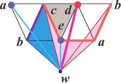
Figure 7.2: A non-manifold $3$-complex where all tetrahedra meet at manifold simplices

Let us consider the (unfolded) Moebius strip in Figure 7.2. This 2-complex is made up of five triangles ($abc$,$bce$,$ced$,$aed$ and $abd$). Next, let us build the cone from $w$ to this triangulation The first thing to note is that vertex $w$ is a non-manifold vertex. In fact, the link of $w$ is a Moebius strip. However, every pair of incident tetrahedra in this cone shares a triangle where just two tetrahedra meet. This can be seen looking at the triangulation of the Moebius strip in Figure 7.2. In this triangulation every triangle incident to an edge with another shares an edge where just two triangles meet. For instance the triangle $cde$ share edge $ce$ with triangle $bce$ and edge $de$ with triangle $ade$. When we take the cone from $w$, we have that the common (red) vertex between two triangles becomes a common edge between two tetrahedra (e.g. the thick edge in violet). Similarly the common (blue) edge becomes a triangle (e.g. the triangle in pale blue). It is easy to see that any pair of tetrahedra in this complex intersect at a manifold simplex. To show this, we first note that the link of the intersection of two triangles in the Moebius strip is the link of a simplex within a manifold (indeed the Moebius strip is a manifold). In particular, when the two triangles shares an edge this link is made up of a couple of points, (e.g. the blue blobs in figure). When the two triangles shares a single vertex this link is a path made up of three consecutive edges (e.g. the the red thick lines in figure). When we take the cone from $w$ we have that the cone to the intersection of two triangles becomes the intersection of two tetrahedra. The cone to the corresponding link becomes the link of the intersection of the two tetrahedra (e.g. the two pale blue edges at $w$ and the three pale red triangles). From the form of these links we can say that any pair of tetrahedra in this complex intersect at a manifold simplex. For this reason, any gluing instruction ${\theta_{1}\leftrightarrow\theta_{2}}$ have a manifold common simplex $\theta={\theta_{1}\cap\theta_{2}}$. Therefore the closed set of instructions that describes this complex is a set of manifold instructions even if the $3$-complex is not a $3$-manifold at point $w$.

So, it is not possible to say that a closed set of manifold instructions will always generate a manifold. Indeed, as we will see in the following, it can be proven that a closed set of manifold instructions generates a quasi-manifold. However, not all quasi-manifold can be generated by closed sets of manifold instructions. Thus, we point out that, the exact characterization of the set of complexes generated by closed sets of manifold gluing instructions is a problem left open by this thesis.

To go on with our study on manifoldness we start by studying some properties of manifold instructions. A first fact is that manifold instructions are regular.

Property 7.3.2.

Manifold instructions are regular instructions. A manifold instruction  cannot be made up of two top simplices of different dimensionality.

Proof 7.3.3.

If ${\theta_{1}\leftrightarrow\theta_{2}}$ is a manifold instruction, then the two top simplices $\theta_{1}$ and $\theta_{2}$ share a simplex $\gamma={\theta_{1}\cap\theta_{2}}$ that must be a manifold simplex in the $d$-complex $\Omega$. By Definition 3.5.6 the link $lk(\gamma)$ must be an $h$-complex (whith $h=d-\dim{\gamma}-1$) that is combinatorially equivalent either to the $h$-sphere or to the $h$-ball. In both cases, by Property 3.5.1 Part 2, we have that $lk(\gamma)$ is an $h$-manifold and hence $lk(\gamma)$ must be a regular $h$-complex. Now $\theta_{1}-\gamma$ and $\theta_{2}-\gamma$ are two simplices in the regular $h$-complex $lk(\gamma)$. Hence $\theta_{1}-\gamma$ and $\theta_{2}-\gamma$ must have the same dimension $h$ and this implies that both $\theta_{1}$ and $\theta_{2}$ have the same dimension. Therefore instruction ${\theta_{1}\leftrightarrow\theta_{2}}$ is a regular instruction.

Manifoldness embodies some notion of regularity. Indeed the location of top simplices around a manifold simplex follows a certain pattern. Therefore no surprise if some of the gluing instructions that stitch top simplices around a manifold simplex are redundant. Indeed all manifold instructions $\theta_{1}\leftrightarrow\theta_{2}$ of order smaller than the maximum (note that the maximum is $\dim{(\theta_{i})}-1$) can be neglected. This is one of the consequences of the following property that relate redundant instructions with connectivity (see Definition 3.2.3) in the generated complex.

Property 7.3.3.

Let be $\theta_{1}$ and $\theta_{2}$ two top $d$-simplices in a $d$-complex $\Omega$. Let be ${\theta_{1}\leftrightarrow\theta_{2}}$ a gluing instruction and let be $\gamma=\theta_{1}\cap\theta_{2}$. Then the following facts holds:

1. If $\star{\gamma}$ is $(d-1)$-connected then there exist a set of regular gluing instructions ${\mathcal{E}}_{\gamma}$, of order $(d-1)$, such that ${\theta_{1}\leftrightarrow\theta_{2}}$ is satisfied by $\approx^{{\mathcal{E}}_{\gamma}}$.

2. If $\star{\gamma}$ is $(d-1)$-manifold-connected then the set ${\mathcal{E}}_{\gamma}$ will be a pseudomanifold set of regular instructions.

Proof 7.3.4.

Not to bother the reader we will embed the proof for the case of manifold connected stars (Part 2) into the proof for plain $(d-1)$-connected stars (Part 1). This will be done by adding, when needed by Part 2, the adjectives (manifold) or (pseudomanifold) between parenthesis. The reader should skip this, or read this, depending on which proof she (or he) wants to read.

Being $\star{\gamma}$ a $(d-1)$-(manifold) connected star there exist, for some $n$ a (d-1)-(manifold) path of $n+1$ $d$-simplices $(\theta^{(i)})_{i=0}^{n}$ in $\star{\gamma}$ with $\theta^{(0)}=\theta_{1}$ and $\theta^{(n)}=\theta_{2}$. Let us consider the regular (pseudomanifold) set ${\mathcal{E}}_{\gamma}$ of $n$ gluing instructions of order $(d-1)$ given by: ${\mathcal{E}}_{\gamma}=\{{\theta^{(i)}\leftrightarrow\theta^{(i+1)}}|i=0,\ldots,(n-1)\}$. We have to show that ${\theta_{1}\leftrightarrow\theta_{2}}$ is satisfied by $\approx^{{\mathcal{E}}_{\gamma}}$. In fact, for any $v\in\gamma$, we have that $v\in\theta^{(i)}$ for all $i=0,\dots,n$. Therefore the set of stitching equations associated with ${{\mathcal{E}}_{\gamma}}$ contains the $n$ equations $v_{\theta^{(i)}}\approx v_{\theta^{(i+1)}}$ for all $i=0,\ldots,(n-1)$. Closing with transitivity we have that equation $v_{\theta^{(0)}}\approx v_{\theta^{(n)}}$ must be in $\approx^{{\mathcal{E}}_{\gamma}}$. By construction we have $\theta^{(0)}=\theta_{1}$ and $\theta^{(n)}=\theta_{2}$. Therefore we have that, for any $v\in\gamma$, the equation $v_{\theta_{1}}\approx v_{\theta_{2}}$ is satisfied by $\approx^{{\mathcal{E}}_{\gamma}}$. So the gluing instruction ${\theta_{1}\leftrightarrow\theta_{2}}$ is satisfied by $\approx^{{\mathcal{E}}_{\gamma}}$.

An easy consequence of the property above is that, in a $d$-complex, a manifold instruction of order smaller than $(d-1)$ can be replaced by a set of of manifold instructions of order $(d-1)$. This is stated in the following property.

Property 7.3.4.

Let $\Omega$ be a $d$-complex and let $\theta_{1}\leftrightarrow\theta_{2}$ be a manifold gluing instructionof order strictly smaller than $(d-1)$. Then, there exist a set of manifold gluing instructions ${\mathcal{E}}_{\gamma}$, of order $(d-1)$, such that ${\theta_{1}\leftrightarrow\theta_{2}}$ is satified by $\approx^{{\mathcal{E}}_{\gamma}}$.

Proof 7.3.5.

Let us denote with $\gamma$ the common simplex i.e. $\gamma=\theta_{1}\cap\theta_{2}$. By hypothesis $\gamma$ is a manifold simplex. Therefore $lk(\gamma)$, being combinatorially equivalent to a $h$-sphere or a $h$-ball, is a connected $h$-manifold (with $h$ the dimension of $lk(\gamma)$). By Property 3.5.2 we have that $lk(\gamma)$ is $(h-1)$-manifold connected and therefore $\star{\gamma}$ is $(d-1)$-manifold connected. By applying the previous Property 7.3.3 Part 2 we get the thesis.

7.4 Initial-Quasi-Manifold

Going on with our analysis of complexes generated by sets of manifold instructions we first consider non closed sets of manifold instructions. We first note that non closed pseudomanifold sets of instructions can generate complexes that are neither manifold, nor pseudomanifold. In the following we will give an example of a non-pseudomanifold $3$-complex that can be generated by a non-closed sets of manifold gluing instruction. In general, for $d\geq 3$, it is possible to find a (non closed) set of manifold instructions that generate a $d$-complex that is not even a pseudomanifold. On the other hand, we have seen in Example 7.3.2 that, for $d\geq 3$, there are examples of closed sets of manifold instructions that generate a non-manifold complex.

At this point, one might wonder whether or not sets of manifold instructions can define any meaningful class of complexes. The answer to this question is positive. In fact, in the following, we will show that two different classes of non-manifold complexes, called Quasi-manifold and Initial-Quasi-Manifolds, are created by sets of manifold gluing instructions, depending on whether the set of instructions is closed or not. The first class is the class of Initial-Quasi-Manifolds complexes. Initial-Quasi-Manifolds are generated by non-closed sets of manifold instructions. This class of non-manifold complexes was introduced for the first time in [36] and. it is important to the sequel of this thesis. Indeed since Initial-Quasi-Manifolds characterize the results of our decomposition of non-manifold complexes.

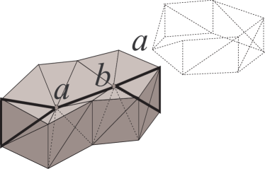
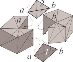
(a) (b)

Figure 7.3: An example of an initial-quasi-manifold complex

Example 7.4.1.

In Figure 7.3a we report a examples of an initial-quasi-manifold complex. Note that the complex is punched at $a$ and $b$. To show this we marked in black a cross section. The complex of Figure 7.3 is an initial-quasi-manifold  $3$-complex. This is not a manifold. In fact, the two central thick Vertices $a$ and $b$ have a link that is not combinatorially equivalent neither to a sphere nor to a disk. The link of vertex $b$ is the dashed surface on the left of Figure 7.3a. Figure 7.3b shows that this complex can be created gluing tetrahedra at manifold triangles. Thus, this complex is generated by a (non-closed) set of manifold gluing instructions of order $2$. These instructions induce the non-manifold gluing instruction ${\theta_{1}\leftrightarrow\theta_{2}}$ of order $1$ (note the two labels 1 and 2 in part b).

Thus in this section we introduce initial-quasi-manifolds as the class of complexes generated by (non-closed) sets of manifold gluing instructions. Next we will characterize initial-quasi-manifolds through local topological properties. In the next section we will show that closed sets of manifold gluing instructions generate the known class of Quasi-manifold introduced by Lienhardt [80].

We start this section introducing an example of a non-pseudomanifold $3$-complex that can be generated by a non-closed pseudomanifold sets of gluing instruction. This correspond to the rather counter intuitive fact there exist non-pseudomanifold $3$-complexes (although not embeddable in ${\rm I\kern-1.99997ptR}^{3}$) that can be generated by glueing together tetrahedra at triangles putting glue on triangles where just two tetrahedra glue at time. In other words non-pseudomanifold adjacency can be induced using the (usual) manifold glue (i.e. manifold adjacencies) on triangles.

Example 7.4.2.

(A non-pseudomanifold $3$-complex generated by glueing at manifold triangles) Here, we present an example of a 3-complex that is not a pseudomanifold and yet it can be generated by a non-closed pseudomanifold sets of instruction. This example is rather complex since it does not admit a geometric embedding in 3D space. Therefore, we describe it as an assembly of pieces that may be built through a pseudomanifold set of gluing $2$-instructions. The general idea is that, while we explicitly glue tetrahedra at manifold triangles, some gluing at non-manifold triangles may be implicitly induced among other faces of such tetrahedra. We first build a pseudomanifold complex that has a cavity that can be filled only through a non-pseudomanifold complex made of three tetrahedra incident at a common triangle. Then, we fill this cavity by gluing new tetrahedra on the cavity boundary. Although each tetrahedron introduced to fill the cavity is glued at three manifold triangles, non-manifold adjacency are induced among such new tetrahedra, and the final complex is necessarily non-pseudomanifold.

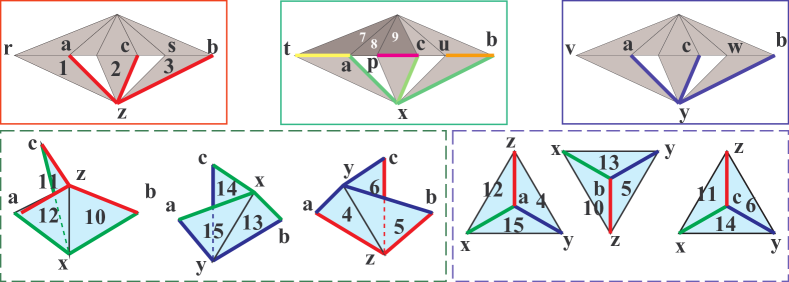
Figure 7.4: A non-pseudomanifold $3$-complex generated by a non-closed pseudomanifold set of $2$-instructions

We start with the 2-complex formed from the three pieces in the first row of Figure 7.4. Such pieces form a connected component since they share three vertices $a$, $b$ and $c$. Each piece contains eight triangles. Then we build the following three cones: from $x$ to the complex on the left (framed in red); from $y$ to the complex in the middle (framed in green); and from $z$ to the complex on the right (framed in blue). Such cones do not share tetrahedra or triangles because the three $2$-complexes in the top row do not share either a triangle or an edge. Therefore, it is easy to see that the resulting complex is a pseudomanifold. The three cones introduce twenty-four tetrahedra. The three cones will share some edges, namely those connecting vertices $x$, $y$ and $z$ to vertices $a$, $b$ and $c$ (thick red, green and blue edges). Due to this fact, the boundaries of the three cones form a closed cavity, which is bounded by the nine incident triangles numbered $4$,$5$,$6$,$10$,$11$,$12$,$13$,$14$ and $15$. On the left side of the second row in Figure 7.4 line) we report these nine triangles organized into three “T”s. Thick red, green and blue edges in the first and second row are shared by the three cones and are on the boundary of this cavity.

Note that additional thick colored lines and some triangle numbering (that now might seem unnecessary) are placed here for later reference. Also the order in which triangles are numbered, that might seem quite arbitrary, is relevant for the second part of this example.

On the right side of the second row in Figure 7.4 we report the same nine triangles organized into three fans of triangles around vertices $a$, $b$ and $c$. From this last presentation, we can see that the three ”T”s form the boundary of a complex made of three tetrahedra $axyz$, $bxyz$ and $cxyz$. Note that the complex we have built so far does not contain these three tetrahedra, while it contains all their faces, except $xyz$. So, we may add such three tetrahedra to the complex through manifold glueing instructions. The resulting complex is non-pseudomanifold since triangle $xyz$ has three incident tetrahedra. The total number of tetrahedra for this complex is twenty-seven. Note that such incidences at $xyz$ were never specified, but implicitly induced, by glueing instructions.

Up to now we have simply detailed the shape of our non-pseudomanifold $3$-complex for this example. The next step is to show that such a complex can be generated by a set on manifold equations of order $2$. More intuitively the question is: can we build this complex by stitching tetrahedra at triangles where only two tetrahedra meet.

This fact can be verified intuitively considering the complex on the left of Figure 7.5. On the left,

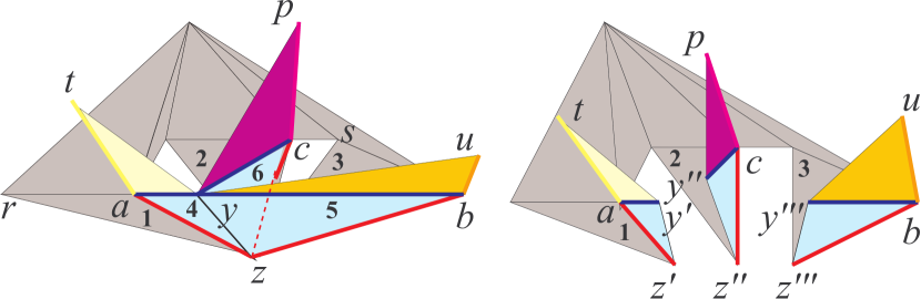
Figure 7.5: How to stitch together $lk(x)$ (on the left) for the complex of Figure 7.4

we have the $2$-complex that is the link of $x$. Pale blue triangles $4$, $5$ and $6$ comes from the three tetahedra added in the cavity. The three colored triangles (yellow,violet and orange) comes from the cone from $y$ to three lines in the complex in the middle of the upper row in Figure 7.4. The triangle in yellow,violet and orange comes from the cone from $y$ to, respectively, the thick yellow,violet and orange edges in the $2$-complex in the middle of upper row of Figure 7.4. Note that, for symmetry, $lk(y)$ and $lk(z)$ must be isomorphic to this complex.

Let us consider the $3$-complex that result from the cone from $x$ to $lk(x)$ (i.e. $\overline{\star{x}}$). This subcomplex cannot be built by stitching together tetrahedra at manifold $2$-faces. However the largest complex we can obtain by stitching together tetrahedra at manifold $2$-faces. is the decomposition obtained as the cone from $x$ to the $2$-complex on the right of Figure 7.5. This takes seven instructions to put in place the gray triangles. Having obtained this complex we start stitching other tetrahedra from $\overline{\star{y}}$ onto it. Note that six tetrahedra from $\overline{\star{y}}$ are already in place. They are the cones from $x$ to the six colored triangles in Figure 7.5. Next we stitch the three tetrahedra, corresponding to the cone from $y$ to the darker triangles $7$, $8$, $9$ in the top row of Figure 7.4. In this way we add four simplex equations. First and last simplex equations are between tetrahedra sharing $tay^{\prime}$ and $pcy^{\prime\prime}$. Others connect the three added tetrahedra. These four simplex equations induce the vertex equation $y^{\prime}\approx y^{\prime\prime}$.

Similarly we consider the four tetrahedra that are cones from $y$ to triangles $10$, $11$, $12$ and $13$. Stitching them from $pcy^{\prime\prime}$ to $uby^{\prime\prime\prime}$ we induce $y^{\prime\prime}\approx y^{\prime\prime\prime}$. Hence by stitching tetrahedra at manifold triangles we build all $\overline{\star{y}}$ and have $y^{\prime}$, $y^{\prime\prime}$ and $y^{\prime\prime\prime}$ collapsing into a unique vertex for $y$.

For symmetry, it is easy to see that, we can consider the triangles $1$, $2$ and $3$ and stitch tetrahedra from $\overline{\star{z}}$ to induce stitching equations $z^{\prime}\approx z^{\prime\prime}$ and $z^{\prime\prime}\approx z^{\prime\prime\prime}$. The whole process stitch together tetrahedra $axy^{\prime}z^{\prime}$, $cxy^{\prime\prime}z^{\prime\prime}$ and $bxy^{\prime\prime\prime}z^{\prime\prime\prime}$ withuot using the non-manifold simplex equations involving $axyz$, $bxyz$ and $cxyz$. This takes twenty-one instructions for the three cones. Finally we introduce nine instructions to fill the cavity for a total of thirty instructions to glue the twenty-seven tetrahedra.

The reader that remains skeptical about this construction could refer to Appendix C where we present a Prolog program for this example. This program details the list ${\mathcal{E}}$ of thirty instructions. Next, the program starts from the totally exploded complex $\Omega^{\top}$ made up of twenty-seven disjoint tetrahedra and execute the list of thirty instructions ${\mathcal{E}}$. At each instruction adjacencies are updated. Finally, when all instruction are executed, the program checks that, in the final complex, $\Omega^{\top}/{\mathcal{E}}$ all tetrahedra join at manifold triangular faces except for a non pseudomanifold triangular face not considered by any instruction in ${\mathcal{E}}$ .

Finally note that taking the cone of from an external vertex to the complex of Example 7.4.2 we can create an example of a 4-complex that is not a pseudomanifold and yet it can be generated by a non-closed pseudomanifold sets of instruction. Then taking again the cone from a fresh new vertex we can create the same sort of example for $d=5$ and so on for all $d\geq 3$.

Even if non-closed set of $(d-1)$ instructions can generate quite wierd complexes it is possible to characterize the set of of regular $d$-complex that can be generated by a non closed set of $(d-1)$-instructions. This characterization is given by the following property that will lead us to the definiton of the class of initial-quasi-manifolds complexes.

Property 7.4.1.

Let $\Omega^{\prime}$ be a complex in the decomposition lattice for a $d$-complex $\Omega$. The following facts hold:

1. If the star of every vertex in $\Omega^{\prime}$ is $(d-1)$-connected then there exist a set of regular $(d-1)$-instructions ${\mathcal{D}}$ such that $\Omega^{\prime}=\Omega^{\top}/{\mathcal{D}}$.

2. If the set ${\mathcal{D}}$ is a set of $(d-1)$-instructions then, in the generated complex $\Omega^{\top}/{\mathcal{D}}$, the star of every vertex is $(d-1)$-connected.

3. If the star of every vertex in ${\Omega^{\prime}}$ is $(d-1)$-manifold-connected then there exist a pseudomanifold set of regular $(d-1)$-instructions ${\mathcal{D}}$, that are manifold w.r.t. $\Omega$, and such that $\Omega^{\prime}=\Omega^{\top}/{\mathcal{D}}$.

4. If the set ${\mathcal{D}}$ is a set of $(d-1)$-instructions that are manifold w.r.t. $\Omega$ then, in the generated decomposition of $\Omega^{\prime}=\Omega^{\top}/{\mathcal{D}}$, the star of every vertex is $(d-1)$-manifold-connected.

Proof 7.4.3.

Let us consider a complex ${\Omega^{\prime}}=\Omega^{\top}/{\mathcal{E}}$ such that the star of every vertex is $(d-1)$-connected. We will show that we can delete in ${\mathcal{E}}$ every gluing instruction provided that we add a certain set of $(d-1)$-instructions. This will prove Part 1. We will also show that this added set can be a set of manifold instructions provided that the star of every vertex in ${\Omega^{\prime}}$ is $(d-1)$-manifold-connected w.r.t. ${\Omega^{\prime}}/R^{\top}$. This will prove Part 3. Not to bother the reader we will embed the proof for the case of manifold connected stars (Part 3) into the proof for plain $(d-1)$-connected stars (Part 1). This will be done, as already done in proof of Property 7.3.3, by adding in some places the adjective (manifold) between parenthesis. The reader should skip this depending on which proof she (or he) is interested in.

Let $\theta_{1}\leftrightarrow\theta_{2}$ be the instruction to be deleted and let be $\gamma=\theta_{1}\cap\theta_{2}$ the common simplex. Let be $v$ a generic vertex in $\gamma$. For this generic vertex $v$ we will provide a set of $(d-1)$ (manifold) gluing instructions ${\mathcal{D}}_{v}$ that satisfy the stitching equation $v_{\theta_{1}}\approx v_{\theta_{2}}$ (one of those added by $\theta_{1}\leftrightarrow\theta_{2}$). To build ${\mathcal{D}}_{v}$, we start by noticing that both $\theta_{1}$ and $\theta_{2}$ belongs to $\star{v}$. The star of $v$ is $(d-1)$-connected in the decomposition, ${\Omega^{\prime}}$. However, pasting ${\Omega^{\prime}}$ with the relation $R^{\top}$ we do not impair $(d-1)$-connectivity. Indeed from ${\Omega^{\prime}}$ to ${\Omega^{\prime}}/R^{\top}$ there an abstract simplicial map that preserve simplex dimension thus preserving $(d-1)$-paths. Therefore the star of any vertex is $(d-1)$-connected in ${{\Omega^{\prime}}/R^{\top}}=\Omega^{\top}/R^{\top}\cong\Omega$. So the star $star({v},{\Omega})$ must be $(d-1)$-(manifold)-connected.

Now we are considering $star({v},{\Omega})$. By hypothesis this star is $(d-1)$-(manifold)-connected. Then we can find a $(d-1)$-(manifold) path $(\theta^{(i)})_{i=1}^{n}$ in $\star{v}$ made up of $n$ $d$-simplices $\theta^{(i)}$. From this path let us build the set of $n-1$ (manifold) instructions. ${\mathcal{D}}_{v}=\{{\theta^{(i)}\leftrightarrow\theta^{(i+1)}}|i=1,\ldots,(n-1)\}$. Proceeding as in the proof of Property 7.3.3 we will find that the set of stitching equations associated with ${\mathcal{D}}_{v}$ contains the $n-1$ equations $v_{\theta^{(i)}}\approx v_{\theta^{(i+1)}}$ with $i=1,\ldots,(n-1)$. Closing with transitivity we have that equation $v_{\theta^{(1)}}\approx v_{\theta^{(n)}}$ must be in $\approx^{{\mathcal{D}}_{v}}$. Being the start and the end of the path respectively $\theta_{1}$ and $\theta_{2}$ we have that equivalence $\approx^{{\mathcal{D}}_{v}}$ satisfy $v_{\theta_{1}}\approx v_{\theta_{2}}$. Summing the sets of the form ${{\mathcal{D}}_{v}}$, for all $v\in\theta$, we will obtain a set of $(d-1)$ (manifold) instructions ${{\mathcal{D}}_{\theta}}=\cup_{v\in\theta}{{{\mathcal{D}}_{v}}}$ such that, for all $v\in\theta$, the stitching equation $v_{\theta_{1}}\approx v_{\theta_{2}}$ must be in $\approx^{{\mathcal{D}}_{\theta}}$. Therefore $\theta_{1}\leftrightarrow\theta_{2}$ is satisfied by $\approx^{{\mathcal{D}}_{\theta}}$.

Iterating this process we can delete from ${\mathcal{E}}$ all instructions of order smaller that $(d-1)$. This completes the proof in the case of plain $(d-1)$ connected stars (Part 1). If we are in the case of manifold connected stars we can use this process also to delete non manifold gluing instructions of order $(d-1)$. If the star of every vertex is $(d-1)$-(manifold)-connected then the added instructions, using the previous construction. can be manifold instructions. Note that, in this second case, by Property 7.2.4, the resulting set of $(d-1)$ instructions, being a set of manifold instructions, is also a pseudomanifold set of instructions. This completes the proof of Part 3.

Parts 2 and 4 can be proven by induction the number $|{\mathcal{D}}|$ of gluing instructions in ${\mathcal{D}}$. As for the first two parts we merge the proofs of these last two parts by adding the adjective (manifold) between parenthesis. This inductive proof is technically possible if we prove the following, stronger, result.

Lemma 7.4.4.

In each $(d-1)$-(manifold)-connected star of a vertex $star({v},{\Omega^{\top}/{{\mathcal{D}}}})$, for two given $d$-simplices in the vertex star: ${\theta^{\top}_{1}}/{\mathcal{D}}$ and ${\theta^{\top}_{n}}/{\mathcal{D}}$, the $(d-1)$-(manifold)-path $({\theta^{\top}_{i}}/{\mathcal{D}})_{i=1}^{n}$ can be selected such that the set of gluing instructions $\{{\theta_{i}\leftrightarrow\theta_{i+1}}|i=1,\ldots,(n-1)\}$ is within ${\mathcal{D}}$.

We start with the inductive basis i.e. we assume $|{\mathcal{D}}|=0$. If $|{\mathcal{D}}|=0$ we have that ${\mathcal{D}}=\emptyset$ and the generated complex is $\Omega^{\top}/\emptyset\cong\Omega^{\top}$. This complex, being a collection of disjoint simplices, satisfy the thesis.

Now let us consider the inductive step. Let be ${\mathcal{D}}={{\mathcal{D}}^{\prime}}\cup\{\theta_{1}\leftrightarrow\theta_{2}\}$ and let us assume that the generated complex $\Omega^{\top}/{{\mathcal{D}}^{\prime}}$ satisfy the thesis. We have to prove that the thesis remains true adding the last gluing instruction $\theta_{1}\leftrightarrow\theta_{2}$. We recall that adding a gluing instruction $\theta_{1}\leftrightarrow\theta_{2}$ we actually add a set of associated stitching equations of the form $v_{\theta_{1}}\approx v_{\theta_{2}}$, one for any $v\in\theta_{1}\cap\theta_{2}$. These stitching equations act on the complex $\Omega^{\top}/{{\mathcal{D}}^{\prime}}$. We have to check that Vertices that are affected do still have a star that is $(d-1)$-(manifold)-connected. Let be $\theta_{1}\leftrightarrow\theta_{2}$ the instruction  to be added and let be $v_{\theta_{1}}\approx v_{\theta_{2}}$ an associated stitching equations not already satisfied by $\approx^{{\mathcal{D}}^{\prime}}$. If such a new equation do not exist the addition of $\theta_{1}\leftrightarrow\theta_{2}$ do not change $\approx^{{\mathcal{D}}^{\prime}}$ and therefore $\Omega^{\top}/{{\mathcal{D}}^{\prime}}=\Omega^{\top}/{{\mathcal{D}}}$ and we are done.

On the other hand, let us assume that there exist an associated stitching equations $v_{\theta_{1}}\approx v_{\theta_{2}}$ not already satisfied by $\approx^{{\mathcal{D}}^{\prime}}$. Adding the gluing instruction $\theta_{1}\leftrightarrow\theta_{2}$, we add the stitching equation $v_{\theta_{1}}\approx v_{\theta_{2}}$, and we cause Vertices ${v_{\theta_{1}}/{{\mathcal{D}}^{\prime}}}$ and $v_{\theta_{2}}/{{\mathcal{D}}^{\prime}}$ to stitch together into the common vertex. Let us call $u$ this common vertex in ${\Omega^{\top}/{{\mathcal{D}}}}$, i.e. $u=v_{\theta_{1}}/{\mathcal{D}}=v_{\theta_{2}}/{\mathcal{D}}$.

For any vertex $v$ we have to prove that $star({v},{\Omega^{\top}/{{\mathcal{D}}}})$ is $(d-1)$-(manifold)-connected via paths that correspond to instructions in ${\mathcal{D}}$. Let us first assume that $v$ is not affected by $\theta_{1}\leftrightarrow\theta_{2}$ and let’s prove that $star({v},{\Omega^{\top}/{{\mathcal{D}}}})$ is $(d-1)$-(manifold)-connected via paths that correspond to instructions that are already in ${\mathcal{D}^{\prime}}$. By inductive hypothesis we have that the star $star({v/{{\mathcal{D}}^{\prime}}},{\Omega^{\top}/{{\mathcal{D}}^{\prime}}})$ is (d-1)-(manifold)-connected.

Furthermore we recall the fact that, by inductive hypothesis, $star({v/{{\mathcal{D}}^{\prime}}},{\Omega^{\top}/{{\mathcal{D}}^{\prime}}})$ is connected through paths corresponding to instructions in ${{\mathcal{D}}^{\prime}}$. We can say that all these $(d-1)$-paths remains in $(d-1)$-paths in $\Omega^{\top}/{{\mathcal{D}}}$ because (by Property 5.4.1) we have an dimension preserving abstract simplicial map between ${\Omega^{\top}/{{\mathcal{D}}^{\prime}}}$ and $\Omega^{\top}/{{\mathcal{D}}}$. These remains paths corresponding to instructions in ${{\mathcal{D}}^{\prime}}$

(in the case of proof for Part 4 note that these instructions are manifold instructions w.r.t. ${\Omega^{\top}/R^{\top}}$. Therefore the $(d-1)$-simplex between the two top simplices in a manifold gluing instruction by inductive hypothesis must be manifold in ${\Omega^{\top}/{{\mathcal{D}}^{\prime}}}$ and must remain manifold in ${\Omega^{\top}/R^{\top}}$ and thus it must be manifold in ${\Omega^{\top}/{{\mathcal{D}}}}$, see Remark 7.4.5 later in this proof for details on this).

Therefore the star $star({v/{{\mathcal{D}}}},{\Omega^{\top}/{{\mathcal{D}}}})$ remains (d-1)-(manifold)-connected whenever $v$ is not affected by $\theta_{1}\leftrightarrow\theta_{2}$.

Now let us return to the case in which, by adding the gluing instruction $\theta_{1}\leftrightarrow\theta_{2}$, we add the stitching equation $v_{\theta_{1}}\approx v_{\theta_{2}}$, and we cause Vertices ${v_{\theta_{1}}/{{\mathcal{D}}^{\prime}}}$ and $v_{\theta_{2}}/{{\mathcal{D}}^{\prime}}$ to stitch together into the common vertex $u=v_{\theta_{1}}/{\mathcal{D}}=v_{\theta_{2}}/{\mathcal{D}}$.

By inductive hypothesis we have that the stars $star({v_{\theta_{1}}/{{\mathcal{D}}^{\prime}}},{\Omega^{\top}/{{\mathcal{D}}^{\prime}}})$ and $star({v_{\theta_{2}}/{{\mathcal{D}}^{\prime}}},{\Omega^{\top}/{{\mathcal{D}}^{\prime}}})$ are (d-1)-(manifold)-connected. Furthermore we recall the fact that they are connected via paths corresponding to instructions in ${{\mathcal{D}}^{\prime}}$. Reasoning as before we can say that all these $(d-1)$-paths remains $(d-1)$-paths in $\Omega^{\top}/{{\mathcal{D}}}$ and they correspond to instructions in ${{\mathcal{D}}^{\prime}}$ (in the case of proof for Part 4 recall that $(d-1)$-simplex between the two top simplices in this manifold gluing instruction and remains manifold in ${\Omega^{\top}/{{\mathcal{D}}}}$, see Remark 7.4.5 later in this proof). Therefore adding ${\theta_{1}\leftrightarrow\theta_{2}}$ we will map $(d-1)$-(manifold)-paths within $star({v_{\theta_{1}}/{{\mathcal{D}}^{\prime}}},{\Omega^{\top}/{{\mathcal{D}}^{\prime}}})$ and $star({v_{\theta_{2}}/{{\mathcal{D}}^{\prime}}},{\Omega^{\top}/{{\mathcal{D}}^{\prime}}})$ into $(d-1)$-(manifold)-paths in $star({u},{\Omega^{\top}/{{\mathcal{D}}}})$.

Next we will show that top simplices in $star({u},{\Omega^{\top}/{{\mathcal{D}}}})$ are $(d-1)$-(manifold)-connected. This will be done by considering the fact that ${\theta^{\top}_{1}/{\mathcal{D}}}\in star({v_{\theta_{1}}/{{\mathcal{D}}}},{\Omega^{\top}/{{\mathcal{D}}}})$ and ${\theta^{\top}_{2}/{\mathcal{D}}}\in star({v_{\theta_{2}}/{{\mathcal{D}}}},{\Omega^{\top}/{{\mathcal{D}}}})$ must share a manifold $(d-1)$-simplex $\gamma_{12}$ in $\Omega^{\top}/{{\mathcal{D}}}$. Paths going between $star({v_{\theta_{1}}/{{\mathcal{D}}^{\prime}}},{\Omega^{\top}/{{\mathcal{D}}^{\prime}}})$ and $star({v_{\theta_{2}}/{{\mathcal{D}}^{\prime}}},{\Omega^{\top}/{{\mathcal{D}}^{\prime}}})$ can always pass through the manifold ”gate” $\gamma_{12}$ and make $star({u},{\Omega^{\top}/{{\mathcal{D}}}})$ a unique $(d-1)$-(manifold)-connected star. .

With this idea in mind we proceed as follows. We note that, since we added the $(d-1)$-(manifold)-instruction $\theta_{1}\leftrightarrow\theta_{2}$, the two $(d-1)$-simplices $\theta^{\top}_{1}/{\mathcal{D}}$ and ${\theta^{\top}_{2}/{\mathcal{D}}}$ will share, in $\Omega^{\top}/{{\mathcal{D}}}$, a $(d-1)$-(manifold)-simplex. Let us denote with $\gamma_{12}$ this simplex in $\Omega^{\top}/{{\mathcal{D}}}$.

Remark 7.4.5.

(In the hypothesis of Part 4 we can prove that $\gamma_{12}$ is a manifold simplex in $\Omega^{\top}/{{\mathcal{D}}}$ with the following steps. First note that instruction $\theta_{1}\leftrightarrow\theta_{2}$ is manifold w.r.t. $\Omega$. Next we note that there is a dimension preserving abstract simplicial map that maps $\Omega^{\top}/{{\mathcal{D}}}$ into $\Omega^{\top}/R^{\top}\cong\Omega$. This must be also a bijection between top simplices. Therefore no more $d$-simplices will share $\gamma_{12}$ in $\Omega^{\top}/{{\mathcal{D}}}$ than those sharing $\gamma_{12}/R^{\top}$ in $\Omega^{\top}/R^{\top}\cong\Omega$. Since $\gamma_{12}$ is the intersection of $\theta^{\top}_{1}/{\mathcal{D}}$ and ${\theta^{\top}_{2}/{\mathcal{D}}}$ the simplex $\gamma_{12}/R^{\top}$ correspond to $\gamma=\theta_{1}\cap\theta_{2}$ w.r.t. the isomorphism that maps $\Omega^{\top}/R^{\top}$ to $\Omega$. Since just two $d$-simplices are sharing $\gamma$ in $\Omega$ two simplices are sharing $\gamma_{12}/R^{\top}$ in $\Omega^{\top}/R^{\top}\cong\Omega$ and no more than two $d$-simplices share $\gamma_{12}$ in $\Omega^{\top}/{{\mathcal{D}}}$ and so ${\theta^{\top}_{1}/{\mathcal{D}}}$ and ${\theta_{2}/{\mathcal{D}}}$ are manifold adjacent in $\Omega^{\top}/{{\mathcal{D}}}$).

We have proven that the two stars $star({v_{\theta_{1}}/{{\mathcal{D}}}},{\Omega^{\top}/{{\mathcal{D}}}})$ and $star({v_{\theta_{2}}/{{\mathcal{D}}}},{\Omega^{\top}/{{\mathcal{D}}}})$ are $(d-1)$-(manifold)-connected through instructions in ${\mathcal{D}}^{\prime}$. Since ${\theta^{\top}_{1}/{\mathcal{D}}}\in star({v_{\theta_{1}}/{{\mathcal{D}}}},{\Omega^{\top}/{{\mathcal{D}}}})$ and ${\theta^{\top}_{2}/{\mathcal{D}}}\in star({v_{\theta_{2}}/{{\mathcal{D}}}},{\Omega^{\top}/{{\mathcal{D}}}})$, paths going from one star to the other can always pass through the ”gate” $\gamma_{12}$. (In the hypothesis of Part 4 we have proven that this is a manifold $(d-1)$-simplex in $\Omega^{\top}/{{\mathcal{D}}}$.) Thus top simplices in $star({u},{\Omega^{\top}/{{\mathcal{D}}}})$ must form a unique $(d-1)$-(manifold)-connected star.

Paths going from one star to the other can always pass through the ”gate” $\gamma_{12}$ in between ${\theta^{\top}_{1}/{\mathcal{D}}}$ and ${\theta^{\top}_{2}/{\mathcal{D}}}$ and satisfy the additional inductive hypothesis we have introduced. Infact in this case paths ”use” the gluing instruction $\theta_{1}\leftrightarrow\theta_{2}$ in ${\mathcal{D}}$. This complete the proof of the inductive step.

The above property supports the definition of initial-quasi-manifolds through local topological properties. Next we will give a property that gives an alternative characterization in term of gluing instructions.

Definition 7.4.6 (Initial-Quasi-Manifold).

An initial-quasi-manifold $d$-complex is a regular $d$-complex where the star of every vertex is $(d-1)$-manifold-connected.

Initial-Quasi-Manifolds are complexes that are generated by sets of manifold gluing instructions.

Property 7.4.2.

Let $\Omega^{\prime}$ be a complex in the decomposition lattice for a $d$-complex $\Omega$. The complex $\Omega^{\prime}$ is an initial-quasi-manifold decomposition if and only if  there exist a set ${\mathcal{D}}$ of manifold $(d-1)$-instructions w.r.t. $\Omega$ such that $\Omega^{\prime}=\Omega^{\top}/{\mathcal{D}}$.

Proof 7.4.7.

By Property 7.4.1 Part 4 we have that a set of $(d-1)$-manifold instructions w.r.t. $\Omega$ generates a regular $d$-complex where the star of every vertex $(d-1)$-manifold-connected. Thus, by Definition 7.4.6 we have. that the complex $\Omega^{\top}/{\mathcal{D}}$ is an initial-quasi-manifold.

Conversely, by Property 7.4.1 Part 3, we have that any initial-quasi-manifold  decomposition of a $d$-complex $\Omega$ can be generated by a pseudomanifold set of regular $(d-1)$-instructions ${\mathcal{D}}$, that are manifold w.r.t. $\Omega$.

Note that, by Property 7.3.4, in a set of manifold instructions ${\mathcal{M}}$, we can purge instructions of order smaller than $(d-1)$. Therefore, if ${\mathcal{M}}$ is a set of manifold instructions w.r.t $\Omega$, then the complex $\Omega^{\top}/{\mathcal{M}}$ is an initial-quasi-manifold decomposition of the $d$-complex $\Omega$.

It is easy to see that manifolds are initial-quasi-manifolds. Initial-Quasi-Manifoldin dimension two are manifolds. In dimension three initial-quasi-manifolds are neither manifolds nor pseudomanifolds. These facts are summarized in the following property

Property 7.4.3.

The following relations holds between manifolds, pseudomanifolds and initial-quasi-manifolds:

1. The class of manifold complexes is a subclass of initial-quasi-manifold complexes.

2. The class of pseudomanifold 3-complexes is neither a subclass nor a superclass of initial-quasi-manifold 3-complexes.

3. Initial-Quasi-Manifolds are $(d-1)$-manifold connected.

4. The class of $2$-manifolds coincide with the class initial-quasi-manifold . $2$-complexes.

Proof 7.4.8.

To prove part 1 we note that a combinatorial manifold is an initial-quasi-manifold since, by Definition 3.5.2, the link of combinatorial $d$-manifold is either a $(d-1)$-sphere or a $(d-1)$-ball. In both cases the link will be $(d-2)$-manifold-connected. Thus, the closed star of a vertex $v$, being the cone from $v$ to its link, will be $(d-1)$-manifold-connected. Thus, by Definition 7.4.6 we have that a combinatorial $d$-manifold is an initial-quasi-manifold.

Since initial-quasi-manifolds are generated by sets of $(d-1)$-manifold instructions we have that by, Property 7.2.3, each connected component in an initial-quasi-manifold is $(d-1)$-connected. Putting together paths in each $(d-1)$-manifold connected vertex star it is easy to see that initial-quasi-manifold are $(d-1)$-manifold-connected. This proves part 3.

To prove part 4 we recall that the link of every vertex in a initial-quasi-manifold is a $(d-1)$-manifold-connected complex. Therefore, for $d=2$, we have that the link of each vertex is $1$-manifold-connected. This means that the link of a vertex in an initial-quasi-manifold $2$-complex must be a graph that is either a chain or a cycle. By Definition 3.5.2, the link of combinatorial $1$-manifold must be combinatorially equivalent either to a $1$-sphere or a $1$-ball. This proves that the set of initial-quasi-manifold $2$-complexes coincides with the set of $2$-manifolds and is a proper subset of $2$-pseudomanifolds.

To prove part 2 we recall that Example 7.4.2 shows that initial-quasi-manifold $3$-complexes are not a subset of $3$-pseudomanifolds. From part 4 we have that the set of initial-quasi-manifold $2$-complexes are a proper subset of $2$-pseudomanifolds.

If we just take decompositions generated by $(d-1)$ manifold gluing instructions, we obtain a decompositions where ”nearly” all singularities are filtered out. Nevertheless this process preserve a good deal of the connectivity in the original complex. Informally we can say that ”good” connectivity is preserved. These ideas will be developed in the next chapter to define the ”best” non singular decomposition for a complex. The following property, that looks quite technical now, will be fundamental to characterize the structure of the ”best” decomposition for a given complex. Informally we can introduce this property by considering that an initial-quasi-manifold $d$-complex can be defined by a rather small set of top $(d-1)$ gluing instructions. The next propperty states that considering all possible top $(d-1)$ gluing instructions and filtering out singular gluing instructions we still preserve ”good” connectivity.

Property 7.4.4.

Let be $\Omega^{\top}/{\mathcal{D}}$ a decomposition for a $d$-complex $\Omega$. The following facts hold:

1. If the set ${\mathcal{D}}$ is the set of all possible $(d-1)$ gluing instructions then, the two top simplices $\theta^{\top}_{a}/{\mathcal{D}}$ and $\theta^{\top}_{b}/{\mathcal{D}}$ are $(d-1)$-connected in $\Omega^{\top}/{\mathcal{D}}$ if and only if $\theta_{a}$ and $\theta_{b}$ are $(d-1)$-connected in $\Omega$.

2. If the set ${\mathcal{D}}$ is the set of all possible $(d-1)$ gluing instructions that are manifold w.r.t. $\Omega$ then, the two top simplices $\theta^{\top}_{a}/{\mathcal{D}}$ and $\theta^{\top}_{b}/{\mathcal{D}}$ are $(d-1)$-manifold-connected in $\Omega^{\top}/{\mathcal{D}}$ if and only if $\theta_{a}$ and $\theta_{b}$ are $(d-1)$-manifold-connected in $\Omega$.

Proof 7.4.9.

We will prove Part 1 and Part 2. merging the two proofs as the in proof of Property 7.3.3. Proof of Part 2 is obtained by considering the adjective (manifold), that will be placed between parenthesis. The reader should skip or not this depending on which proof is interested in (note that the proof for Part 1 spans the next paragraph and the third, then all the rest of the proof is for Part 2 and is not all italicized or reported in parenthesis).

We will first prove that if $\theta_{a}$ and $\theta_{b}$ are two top simplices $(d-1)$-(manifold)-connected in $\Omega$. then $\theta^{\top}_{a}/{\mathcal{D}}$ and $\theta^{\top}_{b}/{\mathcal{D}}$ are $(d-1)$-(manifold)-connected in $\Omega^{\top}/{\mathcal{D}}$. Now let be $\theta_{a}$ and $\theta_{b}$ two top simplices in $\Omega$. These are $(d-1)$-(manifold) connected if and only if there exist a $(d-1)$-(manifold) path $(\theta_{i})_{i=1}^{n}$ made up of $n$ $d$-simplices $\theta_{i}$ with $\theta_{a}=\theta_{1}$ and $\theta_{b}=\theta_{2}$. From this path let us build the set of $n-1$ gluing (manifold) instructions ${\mathcal{D}}_{v}=\{{\theta_{i}\leftrightarrow\theta_{i+1}}|i=1,\ldots,(n-1)\}$. These must be in ${\mathcal{D}}$ because this contains all (manifold) $(d-1)$-instructions for $\Omega$. Being $\Omega^{\top}/{\mathcal{D}}$ a decomposition of $\Omega$ there is a dimension preserving abstract simplicial map between $\Omega^{\top}/{\mathcal{D}}$ and $\Omega^{\top}/{R^{\top}}$ that is a bijection between top simplices. For this reason ${\theta_{i}}/{\mathcal{D}}$ and ${\theta_{i+1}}/{\mathcal{D}}$ must share a $(d-1)$ complex in $\Omega^{\top}/{\mathcal{D}}$. This completes the first half (i.e. $(d-1)$-connected in $\Omega$ implies $(d-1)$-connected in $\Omega^{\top}/{\mathcal{D}}$ ) of the proof for Part 1.

(To complete the proof for Part 2 we have to note that, being $\Omega^{\top}/{\mathcal{D}}$ a decomposition, the number of $d$-complexes incident to ${\theta_{i}}/{\mathcal{D}}\cap{\theta_{i+1}}/{\mathcal{D}}$, can only be smaller that those incident to $\theta_{1}\cap\theta_{2}$. Therefore, in the hypothesis of Part 2, we have that ${\theta_{i}}/{\mathcal{D}}$ and ${\theta_{i+1}}/{\mathcal{D}}$ must share a $(d-1)$ manifold complex in $\Omega^{\top}/{\mathcal{D}}$. Therefore $(\theta_{i})_{i=1}^{n}$ is a $(d-1)$-manifold path. This complete the first half ot the proof for Part 2)

Conversely, now, we will prove that if $\theta_{a}/{\mathcal{D}}$ and $\theta_{b}/{\mathcal{D}}$ are two $d$-simplices that are $(d-1)$-(manifold)-connected in $\Omega^{\top}/{\mathcal{D}}$ then $\theta_{a}$ and $\theta_{b}$ must be $(d-1)$-(manifold)-connected in $\Omega$. Let be $\theta_{a}/{\mathcal{D}}$ and $\theta_{b}/{\mathcal{D}}$ two top simplices that are just $(d-1)$-connected in $\Omega^{\top}/{\mathcal{D}}$. Being $\Omega^{\top}/{\mathcal{D}}$ a decomposition of $\Omega$ there is a dimension preserving abstract simplicial map between $\Omega^{\top}/{\mathcal{D}}$ and $\Omega^{\top}/{R^{\top}}$ that is a bijection between top simplices. Indeed any $(d-1)$-path in $\Omega^{\top}/{\mathcal{D}}$ is preserved in in $\Omega/R^{\top}\cong\Omega$. This completes the second half of the proof for Part 1.

Next, to complete the proof for Part 2, we have to prove that manifold connectivity in ${\Omega^{\top}/{\mathcal{D}}}$ is preserved in $\Omega/R^{\top}\cong\Omega$. Let be $({\theta^{\top}_{i}}/{\mathcal{D}})_{i=1}^{n}$ a $(d-1)$-manifold path in $\Omega^{\top}/{\mathcal{D}}$ in between $\theta^{\top}_{a}/{\mathcal{D}}$ and $\theta^{\top}_{b}/{\mathcal{D}}$. Let be ${\theta^{\top}_{k}}/{\mathcal{D}}$ and ${\theta^{\top}_{k+1}}/{\mathcal{D}}$ two manifold-adjacent $d$-simplices in this $(d-1)$-manifold-path. Actually it might happen that ${\theta_{k}}$ and ${\theta_{k+1}}$ are not manifold adjacent in $\Omega$. In this case we show that we can find a $(d-1)$-manifold path in between ${\theta_{k}}$ and ${\theta_{k+1}}$ in $\Omega$.

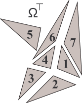
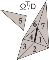
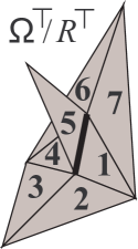
(a) (b) (c)

Figure 7.6: A decomposition $\Omega^{\top}/{\mathcal{D}}$ (b) where a manifold path $(\theta_{1},\theta_{4})$ is no longer a manifold path in $\Omega^{\top}/R^{\top}$ (c)

An example of this situation is shown in Figure 7.6. From the totally exploded version in $\Omega^{\top}$ in Figure 7.6a we obtain the decomposition $\Omega^{\top}/{\mathcal{D}}$ in Figure 7.6b with the set of all manifold gluing instructions ${\mathcal{D}}=\{{\theta_{1}\leftrightarrow\theta_{2}},{\theta_{2}\leftrightarrow\theta_{3}},{\theta_{3}\leftrightarrow\theta_{4}},{\theta_{4}\leftrightarrow\theta_{6}},{\theta_{6}\leftrightarrow\theta_{7}},{\theta_{7}\leftrightarrow\theta_{1}}\}$. In this decomposition the path $(\theta_{1},\theta_{4})$ is a manifold path and is no longer a manifold path in $\Omega^{\top}/{R^{\top}}$. However we can turn around one of the non manifold vertices and obtain back a manifold path, between $\theta_{1}$ and $\theta_{4}$ e.g. with the path $(\theta_{1},\theta_{2},\theta_{3},\theta_{4})$. Such a creation of a new path can be done in general and we will use this fact to prove the thesis.

So the rest of this is to prove Part 2. By Property 1 Part 4, since ${\mathcal{D}}$ is a set of $(d-1)$ manifold instructions, the star of every vertex in $\Omega^{\top}/{\mathcal{D}}$ must be $(d-1)$-manifold connected. Let be $v$ a vertex in ${\theta^{\top}_{k}}/{\mathcal{D}}\cap{\theta^{\top}_{k+1}}/{\mathcal{D}}$. The star $star({v},{\Omega^{\top}/{{\mathcal{D}}}})$ must be $(d-1)$-manifold connected. Therefore there will be a $(d-1)$-manifol-path in $star({v},{\Omega^{\top}/{{\mathcal{D}}}})$ in between the two top simplices ${\theta^{\top}_{k}}/{\mathcal{D}}$ and ${\theta^{\top}_{k+1}}/{\mathcal{D}}$. Now we recall that in the proof of Property 4 Parts 2 and 4 we have proven the following Lemma (see Lemma 7.4.4):

in each $(d-1)$-(manifold)-connected star of a vertex $star({v},{\Omega^{\top}/{{\mathcal{D}}}})$, for two given $d$-complexes in the vertex star: ${\theta^{\top}_{1}}/{\mathcal{D}}$ and ${\theta^{\top}_{n}}/{\mathcal{D}}$, the $(d-1)$-(manifold)-path $({\theta^{\top}_{i}}/{\mathcal{D}})_{i=1}^{n}$ can be selected such that the set of gluing instructions $\{{\theta_{i}\leftrightarrow\theta_{i+1}}|i=1,\ldots,(n-1)\}$ is within ${\mathcal{D}}$.

We apply this result and find a $(d-1)$-manifold-path in $star({v},{\Omega^{\top}/{{\mathcal{D}}}})$ in between ${\theta^{\top}_{k}}/{\mathcal{D}}$ and ${\theta^{\top}_{k+1}}/{\mathcal{D}}$ such that the set of corresponding instructions are in ${\mathcal{D}}$. For this reason these instructions must be manifold w.r.t $\Omega$. This set of instructions trace a $(d-1)$-manifold path in between ${\theta_{k}}$ and ${\theta_{k+1}}$ in $\Omega$. This happens even if ${\theta_{k}}$ and ${\theta_{k+1}}$, are not manifold adjacent in $\Omega$.

Resuming we started with a $(d-1)$-(manifold) path $({\theta_{i}}/{\mathcal{D}})_{i=1}^{n}$ in $\Omega^{\top}/{\mathcal{D}}$. We noted that it can happen that, for some $1\leq k\leq n$, the two top $d$-simplices ${\theta_{k}}$ and ${\theta_{k+1}}$ are not manifold adjacent in $\Omega^{\top}/R^{\top}$. In this case we have shown that we can find a $(d-1)$-manifold path in between ${\theta_{i}}$ and ${\theta_{i+1}}$ in $\Omega$. Therefore $(d-1)$-manifold connectivity is preserved, although possibly through alternative paths, passing from $\Omega^{\top}/{\mathcal{D}}$ to $\Omega/R^{\top}\cong\Omega$. This complete the second half ot the proof for Part 2

7.5 Quasi-manifolds

Quasi-manifolds The problem of characterizing complexes generated by a closed set of manifold instructions will bring in a known family of complexes called quasi-manifold. The informal idea behind this class is that, from the combinatorial point of view the definition of manifold might seem rather arbitrary. In fact there is no reason to privilege the sphere as the canonical form for the link of a vertex. If we just want links to be, somehow, regular we can accept toroidal links or even we can accept the projective plane as a link. This idea leads us to the definition of quasi-manifold. This class was introduced by Lienhardt [80] as the class of complexes modeled by n-G-maps. In this framework we introduce quasi-manifolds by studying complexes generated by a $(d-1)$-closed set of manifold instructions. This will give a new characterization of quasi-manifolds in term of local topologic properties.

We will say that a set ${\mathcal{D}}$ made up of instructions of order $(d-1)$ is $(d-1)$-closed if all the instructions of order $(d-1)$ in ${\mathcal{D}}^{\star}$ are already in ${\mathcal{D}}$. Note that if a $(d-1)$-closed set of $(d-1)$ instructions ${\mathcal{D}}$ generates a $d$-complex $\Omega$ then we can find in ${\mathcal{D}}$ all $(d-1)$ instructions that are satisfied by the equivalence associated to $\Omega$. The following property gives a characterization of complexes generated by a $(d-1)$-closed set of $(d-1)$ manifold instructions.

Property 7.5.1.

A $d$-complex $\Omega$ can be generated by a $(d-1)$-closed set ${{\mathcal{D}}}$ of $(d-1)$-manifold instructions w.r.t. $\Omega$, if and only if, the complex $\Omega$ is a $d$-pseudomanifold where the star of every vertex is $(d-1)$-connected.

Proof 7.5.1.

Let us assume that $\Omega$ can be generated by the $(d-1)$-closed set of $(d-1)$-manifold instructions ${\mathcal{D}}$ and let us prove that $\Omega$ is a pseudomanifold. We have that $\Omega$ can also be generated by the closed set ${\mathcal{D}}^{\star}$. Since all $(d-1)$ instructions in ${\mathcal{D}}^{\star}$ are those in ${\mathcal{D}}$ and since they are all manifold then the set ${\mathcal{D}}^{\star}$ is a closed pseudomanifold set of instructions. Therefore, by Property 7.2.5, the complex generated by ${\mathcal{D}}^{\star}$ is a pseudomanifold. Next we want to prove that in the generated complex $\Omega^{\top}/{\mathcal{D}}$ the star of a vertex $v$ is $(d-1)$-manifold-connected. Infact we have that ${{\mathcal{D}}}$ is a set of $(d-1)$ manifold instructions, therefore, by Property 7.4.1 Part 4, the star of every vertex in the generated complex $\Omega^{\top}/{\mathcal{D}}$ is $(d-1)$-connected.

Conversely, for a given $d$-pseudomanifold $\Omega$ where the star of every vertex is $(d-1)$-connected. we have to build a $(d-1)$-closed set ${{\mathcal{D}}}$ of $(d-1)$ instructions that must be manifold w.r.t. $\Omega$ and s.t. $\Omega^{\top}/{{\mathcal{D}}}\cong\Omega$. By Property 3 Part 4 we have that (an isomorphic copy of) the $d$-complex $\Omega$ can be generated by a set ${{\mathcal{D}}_{0}}$ of $(d-1)$-manifold instructions w.r.t. $\Omega$ (i.e. $\Omega\cong\Omega^{\top}/{{\mathcal{D}}_{0}}$). Let be ${{\mathcal{D}}}$ the set obtained adding to ${{\mathcal{D}}_{0}}$ the other $(d-1)$-instructions that are in ${{\mathcal{D}}_{0}}^{\star}$. Adding the other $(d-1)$-instructions that are in ${{\mathcal{D}}_{0}}^{\star}$ the generated complex do not change. Thus $\Omega^{\top}/{{\mathcal{D}}_{0}}=\Omega^{\top}/{{\mathcal{D}}}\cong\Omega$. By Property 7.2.5, since $\Omega\cong\Omega/{{{\mathcal{D}}_{0}}^{\star}}$ is a pseudomanifold, the set of gluing instructions ${{\mathcal{D}}_{0}}^{\star}$ must be a pseudomanifold set of gluing instructions. By Property 7.2.6 all $(d-1)$ instructions in ${{\mathcal{D}}_{0}}^{\star}$ are manifold w.r.t. $\Omega$. Therefore all $(d-1)$-instructions in the $(d-1)$-closed set ${\mathcal{D}}$ are manifold w.r.t. $\Omega$ and $\Omega^{\top}/{{\mathcal{D}}}\cong\Omega$. This completes the proof.

The above property supports a non constructive definition of quasi-manifold. In fact by the above Property 7.5.1 the following definition is equivalent to that given by Lienhardt in (see the definition of Numbered simplicial quasi-manifolds in [80] Pg. 7 and the discussion in Section 2.2.3).

Definition 7.5.2 (Quasi-manifold).

A $d$-quasi-manifold is a $d$-pseudomanifold where the star of each vertex is $(d-1)$-connected.

From the above definition and from Definition 7.4.6 it is easy to see that quasi-manifolds are a subset of initial-quasi-manifold. By Property 7.4.3 it is easy to see that $2$-quasi-manifolds coincide with initial-quasi-manifold $2$-complexes that in turn coincide with $2$-manifolds. For $d\geq 3$ $d$-quasi-manifolds are a proper superset of $d$-manifolds and a proper subset of $d$-pseudomanifolds. For $d\geq 3$ $d$-quasi-manifolds are a proper subset of initial-quasi-manifold $d$-complexes. This proper inclusion is given by the fact that, for $d\geq 3$, there are initial-quasi-manifold $d$-complexes that are not pseudomanifolds (See Example 7.4.2).

Chapter 8 Standard Decomposition

8.1 Introduction

In Chapter 7 we have developed a classification of complexes generated by a set of gluing instructions ${\mathcal{E}}$. This classification gives some topological properties for the decomposition $\Omega^{\top}/{{\mathcal{E}}}$ on the ground of properties of instructions in ${\mathcal{E}}$. The careful reader may argue that this can be of limited interest speaking about decomposition because (in Example 6.4.2 of Chapter 6 we have seen that) not all decompositions for $\Omega$ can be generated by sets of gluing instruction.

This remark is perfectly legal here because we are not interested in properties of $\Omega^{\top}/{{\mathcal{E}}}$ on its own. We are interested in $\Omega^{\top}/{{\mathcal{E}}}$ as a decomposition of  $\Omega$. This issue, in the first part of this chapter. However note that the results in Chapter 7 might still have some interest if considered on their own. In fact, whenever $\Omega^{\top}/{{\mathcal{E}}}\cong\Omega$, the simplex instructions in ${\mathcal{E}}$ might be regarded as the set of primitive operations modeling $\Omega$. From this point of view results in Chapter 7 gives the topological properties of the resulting complex on the ground of syntactical properties of the set of instructions ${\mathcal{E}}$.

8.2 The Decomposition lattice and gluing instructions

Now let us revert to the decomposition problem. We have seen that gluing instructions cannot generate all decompositions for $\Omega$. In other words sets of gluing instructions are not sufficient to label every path from $\Omega^{\top}$ down to a decomposition $\Omega^{\top}/{\approx}$. However, we can prove that sets of gluing instructions are sufficient to label every path from a decomposition $\Omega^{\top}/{\approx}$ down to $\Omega^{\top}/R^{\top}$. Therefore sets of gluing instructions gives a set of transformations quite meaningful in this context. In fact, here, we focus our attention on the way in which we go from a decomposition $\Omega^{\top}/{\approx}$. down to the original complex $\Omega\cong\Omega^{\top}/R^{\top}$. Next Lemma shows that, for such a focus, we can restrict our attention to paths that can be labeled by sets of gluing instructions.

In particular, we will prove that, for every pair of equating simplices $\nu_{1}$, $\nu_{2}$, in a certain decomposition $\Omega^{\top}/{\approx}$, we can find a gluing instruction  $g=\theta_{1}\leftrightarrow\theta_{2}$ that completely stitch together $\nu_{1}$ and $\nu_{2}$. By completely stitch we mean that adding $\theta_{1}\leftrightarrow\theta_{2}$ to $\approx$ we jump into a decomposition $\Omega^{\top}/{\approx^{\prime}}$ where $\nu_{1}/{\approx^{\prime}}$ and $\nu_{2}/{\approx^{\prime}}$ becomes the same simplex. Furthermore, if at least one of the two equating simplices $\nu_{i}$ is a top equating simplex in $\Omega^{\top}/{\approx}$, then the image of both $\nu_{1}/R^{\top}$ and $\nu_{1}/R^{\top}$ in $\Omega^{\top}/R^{\top}\cong\Omega$ is exactly the common simplex $\gamma^{\bot}=\theta_{1}^{\top}/R^{\top}\cap\theta_{2}^{\top}/R^{\top}$ (i.e. the isomoprhic image in $\Omega^{\top}/R^{\top}\cong\Omega$ of the common simplex $\gamma={\theta_{1}\cap\theta_{2}}$ ”glued” by $\theta_{1}\leftrightarrow\theta_{2}$).

This fact is formally expressed by the following Lemma.

Lemma 8.2.1.

In a decomposition $\Omega^{\top}/\approx$ there exist a pair of distinct equating simplices $\nu_{1}$, $\nu_{2}$ if and only if there exist a gluing instruction $\theta_{1}\leftrightarrow\theta_{2}$ that is not satisfied by $\approx$ and such that the common image of $\nu_{1}$ and $\nu_{2}$ in $\Omega^{\top}/R^{\top}$, (i.e. $\nu_{1}/R^{\top}=\nu_{2}/R^{\top}$) lies within the simplex $\gamma^{\bot}\in\Omega^{\top}/R^{\top}$ corresponding to the common face $\gamma=\theta_{1}\cap\theta_{2}$ in $\Omega$. In symbols it must hold $\nu_{1}/R^{\top}=\nu_{2}/R^{\top}\leq\gamma^{\bot}$ If either $\nu_{1}$ or $\nu_{2}$ is a top equating simplex the their common image in $\Omega^{\top}/R^{\top}$ is exactly $\gamma^{\bot}$.

Proof 8.2.2.

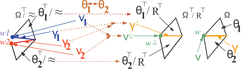
Figure 8.1: Proof of Lemma 8.2.1. Dashed arrows denote the abstract simplicial map induced by a path in the quotient lattice (see Property 4.3.1). All other arrows are used to name objects in the figure. Note that for simplicity, in this particular case, we used equating vertices $w_{1}$ and $w_{2}$ i.e. we take $w_{1}=\nu_{1}$ $w_{2}=\nu_{2}$

A situation coherent with the hypothesis of this Lemma is depicted, just for reference, in Figure 8.1. We first start from the two distinct equating simplices $\nu_{1}$ and $\nu_{2}$ and find a gluing instruction $\theta_{1}\leftrightarrow\theta_{2}$ that is not satisfied by $\approx$ with the properties given in the thesis.

Let $\theta^{\top}_{1}/{\approx}$ and $\theta^{\top}_{2}/{\approx}$ be two top simplices in $\Omega^{\top}/\approx$ that are cofaces of the two equating distinct simplices $\nu_{1}$ and $\nu_{2}$ (in certain complexes several choices are possible for $\theta^{\top}_{i}/{\approx}$ ). Furthermore, we take indices so that $\nu_{i}\leq(\theta_{i}^{\top}/{\approx})$ for $i=1,2$. The top simplices $\theta^{\top}_{1}/{\approx}$ and $\theta^{\top}_{2}/{\approx}$ must be distinct (i.e. cannot be $\theta^{\top}_{1}/{\approx}\textsection=\theta^{\top}_{2}/{\approx}$) because going from a decomposition to another, in particular going from $\Omega^{\top}/{\approx}$ down to $\Omega^{\top}/R^{\top}$, we can not merge two distinct faces $\nu_{1}$ and $\nu_{2}$ within the same top simplex. In fact there is always a dimension preserving map between two decompositions that is a bijection between top simplices (See Definition 5.2.1). Informally, in simple words, this is about assembling not collapsing. The intersection $\gamma=\theta_{1}\cap\theta_{2}$ cannot be empty. In fact the isomorphic copy of $\gamma$ in $\Omega^{\top}/R^{\top}$, denoted by $\gamma^{\bot}$ must contain $\nu_{1}/R^{\top}\cap\nu_{2}/R^{\top}$. To show this note that $\gamma^{\bot}=\theta_{1}^{\top}/R^{\top}\cap\theta_{2}^{\top}/R^{\top}$ and, using $\nu_{i}\leq(\theta_{i}^{\top}/{\approx})$ for $i=1,2$ with identites 4.3.2, it is easy to see that. $\theta_{1}^{\top}/R^{\top}\cap\theta_{2}^{\top}/R^{\top}$ must contain $\nu_{1}/R^{\top}\cap\nu_{2}/R^{\top}$. This proves a part of the thesis. In fact the common image of two equating simplices in $\Omega^{\top}/R^{\top}$, i.e. the simplex $\nu_{1}/R^{\top}=\nu_{2}/R^{\top}$, must be within $\gamma^{\bot}=\theta_{1}^{\top}/R^{\top}\cap\theta_{2}^{\top}/R^{\top}$.

We have proven that the intersection $\gamma=\theta_{1}\cap\theta_{2}$ cannot be empty and therefore $\theta_{1}\leftrightarrow\theta_{2}$ is a gluing instruction for $\Omega$ that stitches together $\nu_{1}$ and $\nu_{2}$. We have to prove that this instruction is not satified by $\approx$. To this aim we note that $\nu_{1}$ and $\nu_{2}$, that are distinct in $\Omega^{\top}/{\approx}$ and thus they must differ for at least two distinct Vertices $w_{1}$ and $w_{2}$ in $\Omega^{\top}/{\approx}$. Let us assume that we take indices so that $w_{i}\in\nu_{i}\leq\theta_{i}^{\top}/{\approx}$ for $i=1,2$. These two vertices must map into a common vertex $w^{\bot}=w_{1}/R^{\top}=w_{2}/R^{\top}$. The common image of two equating simplices in $\Omega^{\top}/R^{\top}$ must be within $\gamma^{\bot}$ and therefore the vertex $w^{\bot}$ must be in $\gamma^{\bot}$. Let $w$ in $\Omega$ be the vertex corresponding to $w^{\bot}$ in $\Omega^{\top}/R^{\top}$. We have that $w\in\gamma$ because $w^{\bot}$ is in $\gamma^{\bot}$. We will show that $\theta_{1}\leftrightarrow\theta_{2}$ is not satisfied by $\approx$ by showing that $w_{\{\theta_{1}\}}\not\approx w_{\{\theta_{2}\}}$. To this aim we note that $w_{i}\in\theta_{i}^{\top}/{\approx}$ for $i=1,2$. Furthermore it must be $w_{\{\theta_{i}\}}/{\approx}\in\theta_{i}^{\top}/{\approx}$ for $i=1,2$. Since $w^{\bot}=w_{i}/R^{\top}=w_{\{\theta_{i}\}}/R^{\top}$ it is impossible that $w_{i}\neq w_{\{\theta_{i}\}}$ otherwise top simplex $\theta_{i}^{\top}/{\approx}$ will decrease its dimension passing from $\Omega^{\top}/{\approx}$ to $\theta_{i}^{\top}/R^{\top}$ in $\Omega^{\top}/R^{\top}$. This is not possible since $\Omega^{\top}/{\approx}$ and $\Omega^{\top}/R^{\top}$ are two decomposition and between top simplices in a decomposition there is always a dimension preserving bijection. Thus $w_{i}=w_{\{\theta_{i}\}}/{\approx}$ Since we know that $w_{1}\neq w_{2}$ we have that $w_{\{\theta_{1}\}}/{\approx}\neq w_{\{\theta_{2}\}}/{\approx}$ and this proves $w_{\{\theta_{1}\}}\not\approx w_{\{\theta_{2}\}}$. This proves $\theta_{1}\leftrightarrow\theta_{2}$ is not satisfied by $\approx$.

Finally w.l.o.g. let us assume that $\nu_{1}$ is a top equating simplex we have to show that $\nu_{1}/R^{\top}=\nu_{2}/R^{\top}=\gamma^{\bot}$. Let us pose $\nu^{\bot}=\nu_{1}/R^{\top}=\nu_{2}/R^{\top}$. We have that $\gamma^{\bot}$ is equal to $\theta_{1}^{\top}/R^{\top}\cap\theta_{2}^{\top}/R^{\top}$ and $\theta_{1}^{\top}/R^{\top}\cap\theta_{2}^{\top}/R^{\top}$ must contain $\nu_{1}/R^{\top}\cap\nu_{2}/R^{\top}=\nu^{\bot}$. Thus we have $\nu^{\bot}\leq\gamma^{\bot}$ Let, for $i=1,2$, $\gamma_{i}$ the face of $\theta_{i}^{\top}/R^{\top}$ s.t. $\gamma_{i}/R^{\top}=\gamma^{\bot}$ this must exist since $\gamma^{\bot}\subset\theta_{i}^{\top}/R^{\top}$. Simplex $\gamma_{i}$ is an equating simplex and being $\nu^{\bot}\leq\gamma^{\bot}$ by remark to Definition 3.3.1 this implies $\nu_{i}\leq\gamma_{i}$ for $i=1,2$. Being $\nu_{1}$ a top equating simplex this cannot be a proper face of an equating simplex, Thus we must have $\nu_{1}=\gamma_{1}$ and thus $\nu_{1}/R^{\top}=\nu_{2}/R^{\top}=\gamma^{\bot}$.

Conversely whenever the equation $\theta_{1}\leftrightarrow\theta_{2}$ is not satisfied by $\approx$ there must be a stitching equation such that $w_{\{\theta_{1}\}}\not\approx w_{\{\theta_{2}\}}$. Thus $w_{\{\theta_{1}\}}/{\approx}\neq w_{\{\theta_{2}\}}/{\approx}$ and yet $w_{\{\theta_{1}\}}/R^{\top}=w_{\{\theta_{2}\}}/R^{\top}$ must be in $\gamma^{\bot}$. Thus taking $\nu_{i}=w_{\{\theta_{i}\}}/{\approx}$ for $i=1,2$ we get the thesis.

In the situation of Lemma 8.2.1 we will say that the gluing instruction $\theta_{1}\leftrightarrow\theta_{2}$ is associated to the equating simplices $\nu_{1}$ and $\nu_{2}$. Note that for a couple of equating simplices there are several different gluing instruction that can be associated. Note, also, that if one of two equating simplices $\nu_{1}$ and $\nu_{2}$ is a top equating simplex not necessarily the other is a top equating simplex, too.

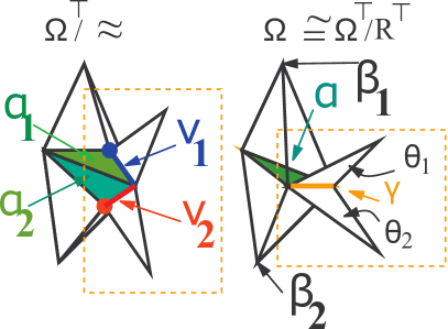
Figure 8.2: An example that shows that the conditions of Lemma 8.2.1 are not sufficient to imply the existience of top equating  simplices.

Example 8.2.3.

Note that the fact that $\nu_{1}/R^{\top}=\theta_{1}^{\top}/R^{\top}\cap\theta_{2}^{\top}/R^{\top}$ do not implies that $\nu_{1}$ is a top equating  simplex. Consider the situation shown in Figure 8.2. In the complex $\Omega$ there is a pair of top 3-simplices $\beta_{1}$ and $\beta_{2}$ such that $\beta_{1}\leftrightarrow\beta_{2}$ is a gluing instruction not satisfied in the decomposition  $\Omega^{\top}/\approx$. In this situation the common simplex $\alpha=\beta_{1}\cap\beta_{2}$ splits in $\Omega^{\top}/\approx$ into two simplices $\alpha_{1}$ and $\alpha_{2}$. Each $\alpha_{i}$, is coface of $\nu_{i}$. Such a situation can be found in the decomposition on the left of Figure 8.2.

In the $3$-complex $\Omega^{\top}/\approx$ we have that the stitching simplices $\nu_{i}$ are non top stitching simplices and is coface of the top stitching triangles $\alpha_{i}$. Note that the pair of simplices $\alpha_{2}$ and $\nu_{1}$ and the gluing instruction  $\beta_{2}\leftrightarrow\theta_{1}$ satisfy the hypothesis of Lemma 8.2.1 and only $\alpha_{2}$ is the top equating simplex between $\alpha_{2}$ and $\nu_{1}$.

Finally note that the pair of top simplices $\nu_{1}$ and $\nu_{2}$ and the gluing instruction $\theta_{1}\leftrightarrow\theta_{2}$ satisfy the hypothesis of Lemma 8.2.1. In this situation the common image of $\nu_{1}$ and $\nu_{2}$ in $\Omega^{\top}/R^{\top}$ is isomorphic to $\gamma=\theta_{1}\cap\theta_{2}$. Thus all the condition in the hypothesis and in the thesis of Lemma 8.2.1 are verified and yet neither $\nu_{1}$ nor $\nu_{2}$ are top equating simplices.

In order to introduce the central theorem in this thesis (Theorem 8.3.4) we present a second lemma that gives more details on the relation between manifoldness of the stitching simplex and manifoldness of the associated simplex instruction $\theta_{1}\leftrightarrow\theta_{2}$. Indeed, by Lemma 8.2.1, for each equating simplex $\gamma^{\prime}$ in $\Omega^{\top}/\approx$ there exist at least one associated gluing instruction $\theta_{1}\leftrightarrow\theta_{2}$ such that this equation is not satisfied by $\approx$ and the pasted version of $\gamma^{\prime}$ is contained in $\gamma^{\bot}=\theta_{1}^{\top}/R^{\top}\cap\theta_{2}^{\top}/R^{\top}$. Note that there are several different gluing instruction with this properties that can be associated.

Lemma 8.2.4.

Let be $\nu^{\prime}$ an equating simplex in $\Omega^{\top}/\approx$ then there exist at least one associated gluing instruction  $\theta_{1}\leftrightarrow\theta_{2}$ such that the following facts holds:.

1. if $\nu^{\prime}$ is a manifold equating simplex the associated gluing instruction must be manifold.

2. if $\nu^{\prime}$ is a top non manifold equating  simplex then the associated gluing instruction must be non-manifold.

3. For each manifold gluing instruction $\theta_{1}\leftrightarrow\theta_{2}$ not satisfied by $\approx$ there exist a manifold equating  simplex $\nu^{\prime}$ in $\Omega^{\top}/{\approx}$ such that $\theta_{1}\leftrightarrow\theta_{2}$ can be associated to $\nu^{\prime}$.

4. For each non manifold gluing instruction  $\theta_{1}\leftrightarrow\theta_{2}$ not satisfied by $\approx$ there exist a non manifold equating  simplex $\nu^{\prime}$ in $\Omega^{\top}/{\approx}$ such that $\theta_{1}\leftrightarrow\theta_{2}$ can be associated to $\nu^{\prime}$.

Proof 8.2.5.

In the proof of Lemma 8.2.1 we have seen (Refer to Figure 8.1 and assume, for instance, $\nu^{\prime}=\nu_{1}$) that the pasted version of an equating simplex $\nu^{\prime}$ is within (an isomorphic copy of) $\gamma=\theta_{1}\cap\theta_{2}$ in $\Omega^{\top}/R^{\top}$. The pasted version is exactly $\gamma^{\bot}$ if $\nu^{\prime}$ is a top equating simplex. This proves part 2. If $\nu^{\prime}$ is not top then its pasted version is a face of $\gamma^{\bot}$. We prove Part 1 since it can be proved (see Remark 3.5.9) that a coface of a manifold simplex is a manifold simplex too.

To prove the remaining two parts we note that we can take for $\nu^{\prime}$ an equating simplex (e.g. $\gamma_{1}$ in Figure 8.1) whose pasted version will be $\gamma^{\bot}$. This will proof Part 3 and Part 4

Note that in general the coface of a manifold simplex is a manifold simplex while the face of a non-manifold simplex is a non-manifold simplex (see Property 3.5.1 Part 4). On the other hand the face of a manifold simplex need not to be a manifold simplex and also the coface of a non-manifold simplex need not to be a non-manifold simplex.

Example 8.2.6.

As a comment to results in Lemma 8.2.4, we present some counterexamples to claims obtained by slight (and wrong) variatons of some of the properties in the above Lemma. The counterexamples are shown in the three Figures 8.3a, 8.3b, 8.3c. In each figure we represent on the left the complex $\Omega^{\top}/\approx$. In this complex we label with $1$ and $2$, the pair of top simplices corresponding to the top simplices $\theta_{1}$ and $\theta_{2}$ mentioned in Lemma 8.2.4. In the complex on the left of each figure the red dot represents the stitching simplex $\nu^{\prime}$. On the right of each figure we present the final complex $\Omega^{\top}/{\approx+\{\theta_{1}\leftrightarrow\theta_{2}\}}$. In the complex on the right of each figure the red dot stands for the pasted version of $\nu^{\prime}$ in $\Omega^{\top}/{\approx+\{\theta_{1}\leftrightarrow\theta_{2}\}}$. Similarly labels $1$ and $2$ are used for the pasted version of simplices $\theta_{1}$ and $\theta_{2}$. With this conventions the three figures show that all the claims below are false.

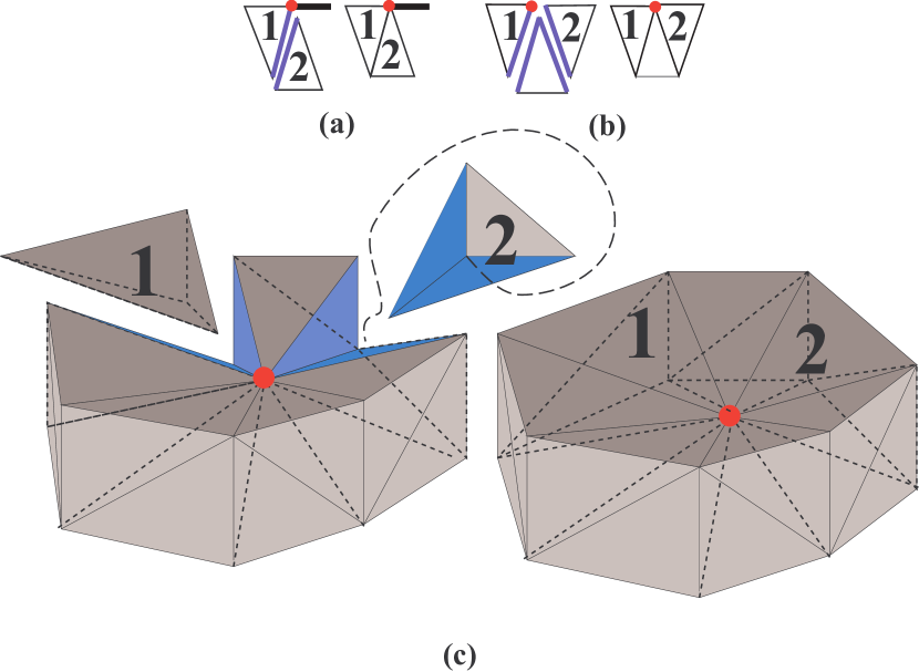
Figure 8.3: Counter examples to some claims about manifold and non manifold stitching simplices

Wrong variation of Part 2 of Lemma 8.2.4

if $\nu^{\prime}$ is a (forget top) non manifold stitching simplex then the associated gluing instruction must be non-manifold.

Indeed in Figure 8.3a the red dot is a non top, non manifold, stitching simplex. The red dot is a face of the blue edge that is a manifold stitching simplex. The claim is wrong because in the complex on the left we can only associate the red dot to the manifold gluing instruction  $\theta_{1}\leftrightarrow\theta_{2}$

Wrong variaton of Part 3 of Lemma 8.2.4

For each manifold gluing instruction $\theta_{1}\leftrightarrow\theta_{2}$ not satisfied by $\approx$ there exist a top (added top) manifold stitching simplex $\nu^{\prime}$ in $\Omega^{\top}/{\approx}$ associated to $\theta_{1}\leftrightarrow\theta_{2}$.

Indeed in Figure 8.3b the top simplices in the gluing instruction $\theta_{1}\leftrightarrow\theta_{2}$ intersect at the red dot that is a non top manifold stitching simplex. Top manifold stitching simplices are the blue edges

Wrong variaton of Part 4 of Lemma 8.2.4

For each non manifold gluing instruction  $\theta_{1}\leftrightarrow\theta_{2}$ not satisfied by $\approx$ there exist a (add top) top non manifold stitching simplex $\nu^{\prime}$ in $\Omega^{\top}/{\approx}$ associated to $\theta_{1}\leftrightarrow\theta_{2}$

Indeed in Figure 8.3c the gluing instruction $\theta_{1}\leftrightarrow\theta_{2}$ is a non manifold gluing instruction. The red dot is the unique non manifold stitching simplex. Furthermore the red dot is the unique stitching simplex to which $\theta_{1}\leftrightarrow\theta_{2}$ can be associated. Some other stitching simplices are the triangles in blue. The 3-simplex numbered 2 is represented turned upside down to show these manifold stitching 2-faces. You have to turn it following the dashed line before stitching it. So the red dot is a non top stitching simplex. The red dot is an example of a non manifold stitching simplex that is face of a top manifold stitching simplex

8.3 Standard decomposition

Usually one perceives pasted non manifold top stitching simplices as ”joints” and seems reasonable to expect to build a decomposition by splitting the complex at non manifold joints. In this section we formalize this concept of ”reasonable” decomposition and show, in Theorem 8.3.4, that the set of such decompositions admits a least upper bound that is made up of initial-quasi-manifold complexes. A consequence of this result will be that, in general, it is not possible to decompose $d$-complexes breaking the complex only at non manifold simplices and expect to obtain manifold connected components. Indeed neither pseudomanifolds connected components can be assured. This is true for all $d\geq 3$. On the other hand a decomposition into manifold components exists for non-manifold surfaces.

Actually it is not possible even to decide if a certain $d$-complex admit a decomposition into $d$-manifold components for all $d$. This fact is an easy consequence of the non recognizability of $d$-manifolds for $d\geq 6$ (see Theorem 3.5.3)

Property 8.3.1.

It is not possible, for $d\geq 6$, to build an algorithm that takes as input an abstract simplicial $d$-complex $\Omega$ and decompose it if and only if  $\Omega$ is non-manifold.

Proof 8.3.1.

Such an algorithm can be used to recognize manifolds simply checking if its output is equal or isomorphic to its input. Thus this algorithm do not exist for $d\geq 6$.

8.3.1 Essential decompositions

An assumption underlying this work is that we are interested in decompositions that splits the original complex only at non manifold simplices. We will call this kind of decomposition an essential decompositions. Since we split at non manifold joint it seemed plausible that decomposition components for essential decompositions must be manifold. This is not always the case. Actually there are complexes for which an essential decomposition with manifold components do not exist. We start the discussion of these problems with the definition of essential decomposition.

Definition 8.3.2 (Essential Decomposition).

A decomposition $\Omega^{\prime}$ will be called an essential decomposition for $\Omega$ if and only if all top equating simplices in $\Omega^{\prime}$ are non-manifold.

We recall that $\gamma^{\prime}$ is a non manifold stitching simplex iff its pasted version is a non manifold simplex. in $\Omega$

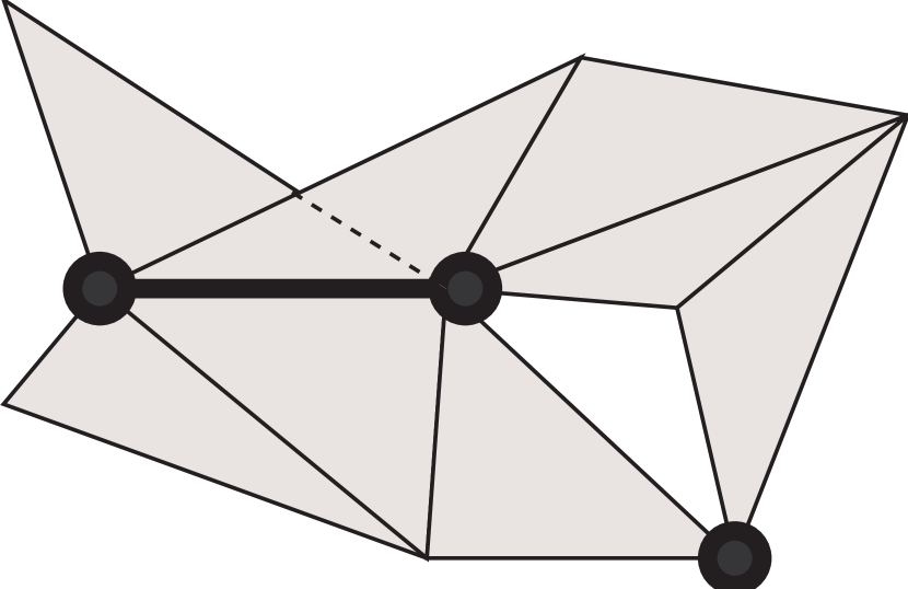
(a)

(b)

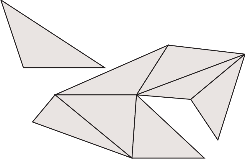
(c)

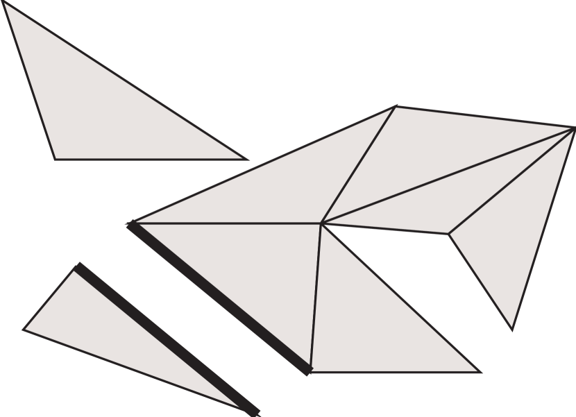
(d)

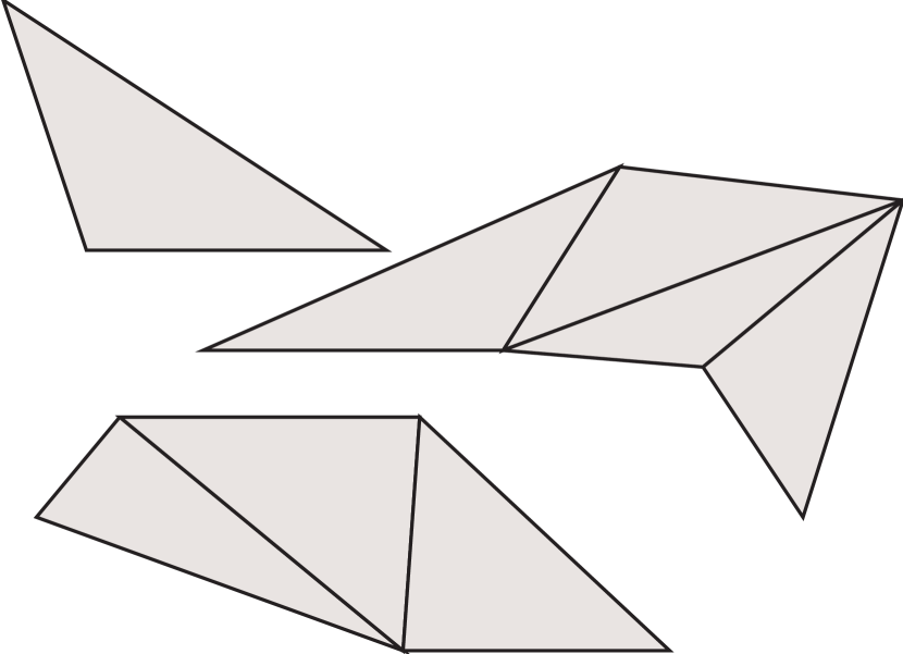
(e)

Figure 8.4: Four decomposition of the complex (a) Decompositions in (b), (c) and (e) are essential, decomposition in (d) is not

Example 8.3.3.

In Figure 8.4 we present three decompositions of the complex in (a). Thick dots and the thick edge in figures (a) and (b) are non manifold simplices. Decomposition in Figure (b) is essential but is still a non manifold complex. Decomposition in Figure (c) and (e) are essential decomposition and connected components are a manifold complex. Decomposition in Figure (d) is a manifold complex but is not a essential decomposition because we split along the thick black edge that is manifold.

A nice property of essential decompositions is that they allow us to define a standard decomposition among essential ones. This decomposition, in some sense, is the ”most general” decomposition among those that are essential. This is expressed by the following theorem that is the main result of this thesis.

Theorem 8.3.4.

Among decompositions for $\Omega$ there exist a unique (up to isomorphism) essential decomposition complex $\nabla\cdot{\Omega}$ that is bigger in the Decomposition Lattice than any other essential decomposition complex. We will call $\nabla\cdot{\Omega}$ the standard decomposition for $\Omega$.

Proof 8.3.5.

We first recall that we only need to consider decompositions in the lattice of decompositions (defined in 5.4.1). Indeed, this lattice, by Property 5.4.2, contains an isomorphic copy of any decomposition of $\Omega$.

We prove the existence of a standard decomposition by explicilty building the standard decomposition $\nabla\cdot{\Omega}$ for $\Omega$. Let be ${\mathcal{M}}$ the set of gluing instructions obtained taking all manifold gluing instructions We will show that $\nabla\cdot{\Omega}=\Omega^{\top}/{\mathcal{M}}$.

First of all we show that $\Omega^{\top}/{\mathcal{M}}$ is essential. Let us consider a top equating simplex in $\Omega^{\top}/{\mathcal{M}}$ and show that it is non-manifold. By Lemma 8.2.1 we have that for every top equating simplex $\gamma^{\prime}$ in $\Omega^{\top}/{\mathcal{M}}$ we can find a gluing instruction  $g=\theta_{1}\leftrightarrow\theta_{2}$ such that $g\notin{\mathcal{M}}$ and such that the pasted version of $\gamma^{\prime}$ is exactly $\gamma^{\prime}/R^{\top}=\gamma^{\bot}=\theta_{1}^{\top}/R^{\top}\cap\theta_{2}^{\top}/R^{\top}$. Since $g\notin{\mathcal{M}}$ we have that $g$ is a non manifold gluing instruction and so, by definition 7.2.3 is $\gamma^{\bot}$. Hence any generic top equating simplex $\gamma^{\prime}$ in $\Omega^{\top}/{\mathcal{M}}$ is non-manifold and therefore $\Omega^{\top}/{\mathcal{M}}$ is essential.

Second we show that for any essential decomposition $\Omega^{\top}/{\approx}$ we have $\Omega^{\top}/{\approx}\leq\Omega^{\top}/{\mathcal{M}}$. We will prove this by proving that for every instruction $g\in{\mathcal{M}}$ we have that $g$ is satisfied by ${\approx}$. Therefore we will have that ${\approx^{\mathcal{M}}}{\subset}{\approx}$ and therefore $\Omega^{\top}/{\approx}\leq\Omega^{\mathcal{M}}$. So let be $\Omega^{\top}/{\approx}$ an essential decomposition and let us assume that there exist a manifold gluing instructions $g=(\theta_{1}\leftrightarrow\theta_{2})\in{\mathcal{M}}$ such that $g$ is not satisfied by ${\approx}$. We can derive a contradiction from this assumption. By Lemma 8.2.4 part 3 there must be a manifold equating simplex $\gamma^{\prime}$ such that $\gamma^{\prime}/R^{\top}=\theta_{1}^{\top}/R^{\top}\cap\theta_{2}^{\top}/R^{\top}$. By definition any equating simplex is always a face of a top equating simplex. Therefore $\gamma^{\prime}$ is face of a top equating simplex. $\gamma^{{\prime\prime}}$ in $\Omega^{\top}/{\approx}$ (i.e. $\gamma^{\prime}\leq\gamma^{\prime\prime}$). Thus, by Equation 4.3 in Property 4.3.2 we have $\gamma^{\prime}/R^{\top}\leq\gamma^{\prime\prime}/R^{\top}$ and thus $\gamma^{\prime}/R^{\top}$ must be face of a $\gamma^{\prime\prime}/R^{\top}$. Being $\Omega^{\top}/\approx$ essential we have that $\gamma^{\prime\prime}$ is a non-manifold equating simplex and therefore $\gamma^{\prime\prime}/R^{\top}$ is a non-manifold simplex is $\Omega^{\top}/R^{\top}$. Faces of a non manifold simplex are non manifold and so must be $\gamma^{\prime}/R^{\top}$. This results in a contradiction since $\gamma^{\prime}$ is a manifold stitching simplex. Hence for all $g\in{\mathcal{M}}$ we have that $g$ is satisfied by ${\approx}$. Therefore, ${\approx^{\mathcal{M}}}{\subset}{\approx}$ and therefore $\Omega^{\top}/{\approx}\leq\Omega^{\mathcal{M}}$.

This proves that is the l.u.b. of the set of essential decompositions. Uniqueness then comes from the fact that the set of all decomposition is a lattice.

In the example of Figure 8.4 the decomposition in (d) is the standard decomposition for the complex in (a).

Theorem 8.3.4 proves that the standard decomposition is the least upper bound among essential decomposition. Indeed, it might happen that more interesting decomposition exist ”below” the standard decomposition. For instance, decomposing particular surfaces, we can have decompositions with larger manifold connected components. For instance in Figure 8.4 we have that the complex in figure (d) is the standard decomposition of the complex in figure (a). Yet the complex of figure (b) is a decomposition obtained by further stitching of the standard decomposition with just two manifold connected components instead of the three in figure (d). However the reduction of these connected components is, somehow, arbitrary. Indeed, in general, if there exist an essential decomposition $\nabla^{\prime}$ strictly smaller than ${\nabla\cdot{\Omega}}$ (i.e. $\nabla^{\prime}<{\nabla\cdot{\Omega}}$) there must be another essential decomposition $\nabla^{\prime\prime}$ that cannot be compared against $\nabla^{\prime}$ and such that $\nabla^{\prime\prime}<{\nabla\cdot{\Omega}}$. In this sense the two essential decomposition $\nabla^{\prime}$ and $\nabla^{\prime\prime}$ are two arbitrary options (i.e. neither $\nabla^{\prime}<\nabla^{\prime\prime}$ nor $\nabla^{\prime\prime}<\nabla^{\prime}$). This is expressed by the following Property

Property 8.3.2.

Let $\nabla^{\prime}$ be a essential decomposition of $\Omega$ in the decomposition lattice such that ${\Omega^{\top}/R^{\top}}<\nabla^{\prime}<\nabla\cdot{\Omega}$. In this situation, in the decomposition lattice there always exist another essential decomposition $\nabla^{\prime\prime}\neq\nabla^{\prime}$ such that the following diagram holds in the decomposition lattice:

$$\begindc{\commdiag}[500]\obj(1,1)[b]{\mbox{\large$\nabla\cdot{\Omega}$}}\par\par\obj(0,0)[a1]{\mbox{\large$\nabla^{\prime}$}}\obj(2,0)[c1]{\mbox{\large$\nabla^{\prime\prime}$}}\par\obj(1,-1)[b2]{\mbox{\large$\Omega^{\top}/R^{\top}$}}\par\par\mor{b}{a1}{}\mor{b}{c1}{}\mor{a1}{b2}{}\mor{c1}{b2}{}\enddc$$

In the diagram at right below, all arrows have the (def i.e. ${\Omega^{\top}/R^{\top}}<\nabla^{\prime\prime}<\nabla\cdot{\Omega}$

Proof 8.3.6.

We can write $\nabla\cdot{\Omega}$ as $\Omega^{\top}/E$ for some set of stitching equations $E$. We can write $\nabla^{\prime}$ as $\Omega^{\top}/(E+E^{\prime})$ for some additional set of stitching equations $E^{\prime}$ and we can write ${\Omega^{\top}/R^{\top}}$ as $\Omega^{\top}/(E+E^{\prime}+E^{\prime\prime})$ for some additional set of stitching equations $E^{\prime\prime}$. Since the . Similarly (see section A.5 in Appendix A). By semimodularity we can draw the diamond:

$$\begindc{\commdiag}[500]\obj(1,1)[b]{\mbox{\large$E+E^{\prime}+E^{\prime\prime}$}}\par\par\obj(0,0)[a1]{\mbox{\large$E^{\prime}$}}\obj(2,0)[c1]{\mbox{\large$E^{\prime\prime}$}}\par\obj(1,-1)[b2]{\mbox{\large$E$}}\par\par\mor{b}{a1}{}\mor{b}{c1}{}\mor{a1}{b2}{}\mor{c1}{b2}{}\enddc$$

We obtain the diamond in the thesis taking all the quotients of $\Omega^{\top}$ w.r.t. the sets of stitching equations: $E$, $E^{\prime}$, $E^{\prime\prime}$, $E+E^{\prime}+E^{\prime\prime}$ and naming. $\nabla^{\prime\prime}$ the quotient $\Omega^{\top}/E^{\prime\prime}$

Thus, the decomposition ${\nabla\cdot{\Omega}}$ is the less decomposed complex obtained cutting only at non-manifold simplices. The standard decomposition is an essential decomposition and all other essential decompositions, in different ways, are less decomposed than ${\nabla\cdot{\Omega}}$.

We note that the proof of Theorem 8.3.4 is a constructive proof since it gives a procedure to build the standard decomposition $\nabla\cdot{\Omega}$. This allows to give some properties of the complex $\nabla\cdot{\Omega}$. The first fact about standard decomposition is that this decomposition tears apart features with mixed dimensionality. This is due to the fact that manifold gluing instructions must be regular. This is expressed by the following property:

Property 8.3.3.

The connected components of the standard decomposition $\nabla\cdot{\Omega}$ are regular

Proof 8.3.7.

In the proof of Theorem 8.3.4 We have seen that $\nabla\cdot{\Omega}=\Omega^{\top}/{\mathcal{M}}$ being $M$ a set of manifold gluing instruction. By Property 7.3.2 we have that instructions in ${\mathcal{M}}$ must be all regular. Hence, we can apply Property 7.2.1 and state that connected components of $\Omega^{\top}/{\mathcal{M}}=\nabla\cdot{\Omega}$ must be regular.

A second, deeper, characterization of the complex $\nabla\cdot{\Omega}$ comes from the fact that, to build this complex, we used manifold instructions. The consequence of this fact is that the resulting complex has connected components that are initial-quasi-manifold complexes. This is stated in the following property

Property 8.3.4.

The connected components of the standard decomposition $\nabla\cdot{\Omega}$ are initial-quasi-manifold complexes.

Proof 8.3.8.

In the proof of Theorem 8.3.4 we have seen that $\nabla\cdot{\Omega}=\Omega^{\top}/{\mathcal{M}}$ being $M$ a set of manifold gluing instructions. We have seen in Property 7.3.2 that all manifold instructions must be regular. Therefore we can assign a dimension to instructions in ${\mathcal{M}}$. Let be ${\mathcal{M}}_{h}$ the set of instructions of dimension $h$ in ${\mathcal{M}}$. By Property 7.2.2 we have that connected components of dimension $h$ are all those within the regular $h$-complex $\Omega^{\top}_{h}/{{\mathcal{M}}_{h}}$, where $\Omega^{\top}_{h}$ is the subcomplex of top simplices of $\Omega^{\top}$ of dimension $h$. Since instructions within ${{\mathcal{M}}_{h}}$ are all manifold by repeated application of Property 7.3.4 we can replace all equations of order smaller than $(h-1)$ with some others manifold instructions of order $(h-1)$. The added instructions can generate more identification than the original instruction,but this is not important since we are interested in showing that this process will produce a set of $(h-1)$-manifold instructions ${{\mathcal{M}}^{\prime}_{h}}$ such that ${\Omega^{\top}_{h}/{{\mathcal{M}}^{\prime}_{h}}}={\Omega^{\top}_{h}/{{\mathcal{M}}_{h}}}$. In the end this shows that the connected components of order $h$ can be generated by a set of $(h-1)$-manifold instructions. This implies, by Property 7.4.1 Part 2 that the link of every vertex in ${\Omega^{\top}_{h}/{{\mathcal{M}}_{h}}}$ is $(h-1)$-manifold connected. Therefore each connected component within ${\Omega^{\top}_{h}/{{\mathcal{M}}_{h}}}$ is an initial-quasi-manifold.

We note that there are examples of 3-complexes $\Omega$ for which the decomposition $\nabla\cdot{\Omega}$ is non manifold.

The complex on the right of Figure 8.3 part (c) shows that it is impossible in general to find a decomposition of certain non manifolds $d$-complex by splitting the complex only at pasted non manifold top stitching simplices. In fact the $3$-complex on the right of Figure 8.3c is an initial-quasi-manifold  complex. All simplices but the central (thick red) vertex are manifold simplices. The central vertex is not a manifold vertex because its link is not homeomorphic to a sphere or a triangle. Nevertheless the star of the central vertex is, obviously, a $2$-manifold-connected complex.

Therefore this complex is an initial-quasi-manifold $2$-complex and its standard decomposition is the complex itself. This decomposition is therefore a non-manifold complex. This is not too counter-intuitive since we really do not have a good reason to decide how to break this complex into manifold pieces. Probably intuition suggests to inflate this complex to make it more regular. In fact the standard decomposition of the surface that is the boundary of this complex split the central vertex in two and yields a decomposition homeomorphic to a sphere. We recall, from Example 7.4.2, that there are initial-quasi-manifold $3$-complexes that are not pseudomanifolds and therefore there are standard decompositions for $3$-complexes that are not $3$-pseudomanifolds. Finally we note that being the set of initial-quasi-manifold $2$-complexes equivalent to $2$-manifolds (see Part 4 of Property 7.4.3) it is always possible to decompose $2$-complexes into $2$-manifolds.

8.4 Computing $\nabla\cdot{\Omega}$

A byproduct of the findings in the proof of Property 8.3.4 is the following property that gives a first procedure to build the standard decomposition.

Property 8.4.1.

The standard decomposition $\nabla\cdot{\Omega}$ for a $d$-complex $\Omega$ is generated by the set obtained taking, for all $1\leq h\leq d$, all simplex pairs ${\Pi_{\theta}^{h}}=\{\theta_{1},\theta_{2}\}$ that satisfy the following constraints:

• ${\Pi_{\theta}^{h}}$ is regular of dimension $h$ (i.e. such that $\mbox{\rm dim}{(\theta_{1})}=\mbox{\rm dim}{(\theta_{2})}=h$);

• ${\Pi_{\theta}^{h}}$ is of order $(h-1)$ (i.e. $\mbox{\rm dim}{(\theta_{1}\cap\theta_{2})}=h-1$);

• ${\Pi_{\theta}^{h}}$ is such that the two simplices $\theta_{1}$ and $\theta_{2}$ gives the star of their intersection (i.e. $\star{(\theta_{1}\cap\theta_{2})}=\{\theta_{1},\theta_{2}\}$ ).

The set ${{\mathcal{M}}_{h}}$ of all pairs of dimension $h$ that satisfy the above requirements will generate the regular connected components of dimension $h$. If $\Omega^{\top}_{h}$ is the set of top simplices of dimension $h$ in $\Omega^{\top}$ we have that the $h$-complex $\Omega^{\top}_{h}/{{\mathcal{M}}_{h}}$ is made up of all connected components of dimension $h$ in $\nabla\cdot{\Omega}$.

Proof 8.4.1.

In the proof of Property 8.3.4 we have that each connected component of dimension $h$ is generated by the set of regular $(h-1)$-manifold instructions of dimension $h$ (denoted by ${{\mathcal{M}}_{h}}$). Furthermore in the proof of that property we have noticed that the set of connected $h$-components is given by the complex $\Omega^{\top}_{h}/{{\mathcal{M}}_{h}}$. Since these are manifold instructions only $h$ simplices must be incident to $\theta=\theta_{1}\cap\theta_{2}$. Since $\mbox{\rm dim}{(\theta)}=(h-1)$ only two $h$-simplices must be incident to $\theta$. These two $h$-simplices must be $\theta_{1}$ and $\theta_{2}$.

Property 8.4.1 gives a computable procedure to select a limited number of instructions. By applying these instructions repeatedly to simplices in $\Omega^{\top}$ we can effectively compute the standard decomposition $\nabla\cdot{\Omega}$ by a top down process. If $n$ is the number of top simplices in the $d$-complex $\Omega$ the construction of $\nabla\cdot{\Omega}$ can be done with a time complexity of $O((nd)^{2})$. Infact we simply have to intersect every top simplex with all others to build an incidence relation between top simplices. Each intersection can be done in $O(d^{2})$ and therefore all intersections can be computed in $O((nd)^{2})$ time. For each top $h$-simplex we allocate record with $2^{(h+1)}-1$ entries to store possible incidence at a certain face. When this incidence relation is built, a linear scan of the $n$ records in the relation will inspect all incidence relation for each simplex and select those that must be preserved in $\nabla\cdot{\Omega}$. Since the possible different incidence pairs are $O(n^{2})$ this process takes at most $O(n^{2})$. This accounts for an overall time complexity of $O((nd)^{2})$ and an overall space complexity of $O(n2^{d})$ to store the incidence relation.

This top down construction, from $\Omega^{\top}$ down to $\nabla\cdot{\Omega}$ is only partially satisfactory. Indeed, for several pragmatic reasons, it is interesting to develop a decomposition procedure that splits the original complex and produces the decompostion bottom up by a progressive refinement at different points. Furthermore we want to develop a decomposition procedure that splits a certain vertex $v$ using local topological information round the vertex $v$.

8.5 Computing $\nabla\cdot{\Omega}$ by local editing

In this Section, we present a decomposition algorithm that builds the standard decomposition $\nabla\cdot{\Omega}$ by splitting $\Omega$ at vertices that violate the condition for initial-quasi-manifoldness. The algorithm works iteratively on the vertices of the input complex and recursively on its dimension.

The algorithm for computing $\nabla\cdot{\Omega}$ is given by the pseudocode in the Algorithm 8.5.1. This algorithm defines a recursive procedure ${\rm DECOMPOSE}(\Omega,d)$ that returns the connected components of the standard decomposition for a $d$-complex $\Omega$. In the design of this algorithm we assume that Vertices are coded as distinct positive integers and that each top simplex receive an index that is a positive integer, too. We assume that the complex $\Omega$ is presented in input as a $TV$ map between top simplex and Vertices, We assume to have a function ${\rm CONNECTED\_COMPONENTS}(\Omega_{c})$ that takes the $TV$ representation of a complex $\Omega_{c}$ and returns a set of $TV$ maps one for each connected component of $\Omega_{c}$. Note that we assume that this function need not to change the coding for vertices and top simplices. Similarly we commit not to change this coding when providing the output of ${\rm DECOMPOSE}(\Omega,d)$. We assume that a standard implementation for sets is used by ${\rm CONNECTED\_COMPONENTS}(\Omega_{c})$ to provide its output. As a consequence sets operations are freely used with a rather abstract stlye in the design of the algorithm.

This function starts by initializing a variable $\Omega_{c}$ with a copy of $\Omega$. The $\Omega_{c}$ holds the current decomposition of $\Omega$ and the algorithm splits $\Omega_{c}$ until it contains $\nabla\cdot{\Omega}$. The algorithm considers each vertex $v$ of $\Omega$ and computes recursively the decomposition of the link of $v$ in $\Omega$ (not the link in $\Omega_{c}$). Based on such a decomposition, the algorithm decides whether and how $\Omega_{c}$ should be split at $v$. Recursion stops for $d=0$ since the decomposition of either a $0$-complex, or of an empty complex trivially coincides with the complex itself.

Algorithm 8.5.1 (Computes the connected components in $\nabla\cdot{\Omega}$ for the $d$-complex $\Omega$).

 

1:  function DECOMPOSE($\Omega$,$d$)

2:  $\Omega_{c}\leftarrow\Omega$

3:  if $d>0$ and $\Omega\neq\emptyset$ then

4:     for all vertices $v$ of $\Omega$ do

5:        $LK\leftarrow lk({v},{\Omega})$ {$LK$ is the link of $v$ in $\Omega$}

6:        $h\leftarrow\mbox{\rm dim}(LK)$ {$h$ is the dimension of $LK$}

7:        $L\leftarrow{\rm DECOMPOSE}(LK,h)$ {compute the components of ${\nabla\cdot{LK}}$}

8:        if ($h>0$ and $|L|>1$) or ($h=0$ and $|L|>2$) then {$v$ must split}

9:           for all $\Psi\in L$ do {split $v$ in $\Omega_{c}$}

10:              Create $v_{\Psi}$ {create a new copy $v_{\Psi}$ for $v$}

11:              Replace $v$ with $v_{\Psi}$ in top simplices of $star({v},{\Omega_{c}})$ incident to a simplex in $\Psi$

12:           end for{the decomposition of vertex $v$ has been completed}

13:        end if

14:     end for

15:  end if

16:  return CONNECTED_COMPONENTS($\Omega_{c}$) {returns connected components of $\Omega_{c}$}

 

The general idea at the basis of this algorithm is to test vertices of $\Omega$ for the local property that characterizes initial-quasi-manifolds (i.e. the star of each vertex $v$ of an initial-quasi-manifold must be manifold-connected) and to split the complex in case a vertex violates such a property. The manifold connection of the star of a vertex is ensured iff its link (which has a lower dimension) is manifold-connected. This is true because adding vertex $v$ to all simplices in the link we obtain all and alone the simplices in the closed vertex star. Therefore, we want to decompose the link of $v$ into manifold-connected components. This process induces only all those splits that are necessary to obtain the standard decomposition. Note that the recursive algorithm actually decomposes the link of a vertex into initial-quasi-manifold components rather than manifold-connected components. On the basis of Part 2 in Property 7.4.4 this result is equivalent, for our purposes, because the partition of top simplices among connected components is the same in the two cases.

Property 8.5.1 (Correctness of Algorithm 8.5.1).

Let $\Omega$ be a TV map of an abstract simplicia $d$-complex. The algorithm 8.5.1 terminates and upon completion the function ${\rm DECOMPOSE}(\Omega,d)$ returns a set of TV maps each representing a connected component of $\nabla\cdot{\Omega}$. The function ${\rm DECOMPOSE}(\Omega,d)$ do not change the assignment of indexes given in input.

Proof 8.5.1.

Termination can be proved easily by induction on the dimension of the input $d$-complex $\Omega$. For $d=0$ procedure stops immediately. On the other hand, if $d>0$, the computation performs a finite number of cycles, one for each vertex $v$ in $\Omega$, calling recursively itself to compute the decomposition of link $lk(v)$. Since each link is at most of dimension $(d-1)$, by inductive hypothesis, we can assume that the decomposition of each link completes. Therefore the overall process must complete, too.

The correctness trivially holds for all $d$ whenever $\Omega=\emptyset$ (i.e. $\Omega$ is a map with no entry). Whenever $\Omega\neq\emptyset$ the proof can be done by induction on the dimension $d$ of the complex $\Omega$. If $d=0$ we have $\nabla\cdot{\Omega}=\Omega$ and the property trivially holds, too.

If $d>0$ we assume that the property holds for $d-1$ and show that it holds for $d$. Thus, by inductive hypothesis we have that the call to ${\rm DECOMPOSE}(LK,h)$ returns the set of connected components in the standard decomposition of the link $lk({v},{\Omega})$. By the result in Part 2 in Property 7.4.4 we have that this is equivalent to the partition into manifold connected components of set of top simplices in $lk({v},{\Omega})$. By Property 8.3.4 the components of $\nabla\cdot{\Omega}$ must be initial-quasi-manifold an therefore by Definition 7.4.6 the link of each vertex in $\nabla\cdot{\Omega}$ is manifold-connected. Thus for each vertex $v$ in $\Omega$ the partition of top simplices in $lk({v},{\Omega})$ induced by the decomposition $\nabla\cdot{\Omega}$ is a (possibly identical) further decomposed version of the partition computed by the algorithm 8.5.1. In fact at line 11 we take the cone from the new vertex copy $v_{\Psi}$ to each component of the partition into manifold connected components of $lk({v},{\Omega})$. Thus $\nabla\cdot{\Omega}$ must be a decomposition of the output of ${\rm DECOMPOSE}(\Omega,d)$ (up to isomorphism).

On the other hand the partition of top simplices in $lk({v},{\Omega})$ used by the algorithm is the partition in $\nabla\cdot{lk({v},{\Omega})}$. This complex in general is a decomposition of the complex ${lk({v},{\nabla\cdot{\Omega}})}$. This second complex induces a partition of top simplices in $lk({v},{\Omega})$ that is the partition induced by the decomposition $\nabla\cdot{\Omega}$. Thus this proves that the partition of top simplices in $lk({v},{\Omega})$ induced by the decomposition computed by the algorithm 8.5.1. is a (possibly identical) partition of the decomposition induced by $\nabla\cdot{\Omega}$. Thus the output of ${\rm DECOMPOSE}(\Omega,d)$. must be a decomposition of $\nabla\cdot{\Omega}$.

We have proven both that $\nabla\cdot{\Omega}$ must be a decomposition of ${\rm DECOMPOSE}(\Omega,d)$ and that the output of ${\rm DECOMPOSE}(\Omega,d)$. must be a decomposition of $\nabla\cdot{\Omega}$. This proves that ${\rm DECOMPOSE}(\Omega,d)$ computes an isomorphic copy of $\nabla\cdot{\Omega}$ and this completes the proof .

At an intuitive level we can say that we can obtain the decomposition $\nabla\cdot{\Omega}$ gluing top simplices in $\Omega^{\top}$ using manifold gluing instructions ${\mathcal{M}}$. Indeed the algorithm splits a vertex $v$ in $\Omega$ into a certain number of vertex copies $v_{\Psi}$ to be used in $\nabla\cdot{\Omega}$. Then the stars of all vertex copies $v_{\Psi}$ (i.e. $\overline{star({v_{\Psi}},{\nabla\cdot{\Omega}})}$) can be partially formed from the totally exploded version of $\overline{star({v},{\Omega})}$ applying all manifold gluing instructions of the form $\theta_{1}\leftrightarrow\theta_{2}$ that mention a pair of top simplices in $\overline{star({v},{\Omega})}$.

From the definition of standard decomposition this means that we glue from the totally exploded version of ${\overline{star({v},{\Omega})}}$ down towards $\nabla\cdot{\overline{star({v},{\Omega})}}$ establishing all manifold joints between top simplices in ${\overline{star({v},{\Omega})}}$. Thus the manifold connected components in the stars ${\overline{star({v_{\Psi}},{\nabla\cdot{\Omega}})}}$ and in $\nabla\cdot{\overline{star({v},{\Omega})}}$ must be formed by the same top simplices.

This do not means that the star $\nabla\cdot{\overline{star({v},{\Omega})}}$ and the collection of stars ${\overline{star({v_{\Psi}},{\nabla\cdot{\Omega}})}}$ need to be the same (isomorphic) complex. Actually the links of $v_{\Psi}$ in the standard decomposition can be less decomposed than $\nabla\cdot{lk({v},{\Omega})}$ See for instance the example of Figure

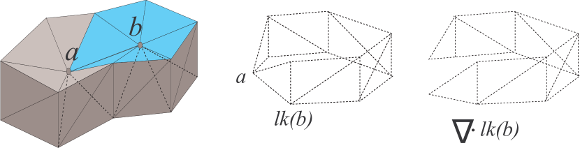
Figure 8.5: An example of a complex where ${\overline{star({b},{\nabla\cdot{\Omega}})}}$ is less decomposed than $\nabla\cdot{lk({b},{\Omega})}$

In Figure 8.5 we report an initial-quasi-manifold complex. This complex is not decomposed be the standard decomposition. Let see why. The link of $b$ in this complex is the dashed surface in the middle of this figure. The $\nabla\cdot{lk({b},{\Omega})}$ is the dashed surface on the right of this figure. It still have one connected component. Therefore we do not split b. The ${\overline{star({b},{\nabla\cdot{\Omega}})}}$ is the complex in pale blue and is less decomposed than $\nabla\cdot{lk({b},{\Omega})}$. The situation for $a$ is similar.

In spite of this example, connecting fresh vertex copies (i.e. ${v_{\Psi}}$ to the connected components of $\nabla\cdot{lk({v},{\Omega})}$ we establish the right number of vertex copies for $v$ and connect them properly to the right component in the link. ${lk({v_{\Psi}},{\nabla\cdot{\Omega}})}$. Doing this for all vertices (as the main cycle of the algorithm does) we get $\nabla\cdot{\Omega}$.

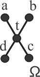
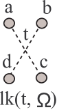
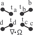
(a)   (b)   (c)

Figure 8.6: An example of the decomposition process for the $1$-complex in (a)

Example 8.5.2.

We illustrate how the algorithm works on some examples in $1$ and $2$ dimensions. Consider first the 1-complex on Figure 8.6a. In this complex, the link of vertices $a$, $b$, $c$ and $d$ is always the vertex $t$ and, thus, the algorithm does not split these four vertices. The link of vertex $t$ is composed of the four gray vertices $a$, $b$, $c$ and $d$ depicted in Figure 8.6b. This is a $0$-complex and is left unchanged, but it consists of four connected components. The algorithm then decides to introduce four copies of $t$, one copy for each connected component in $lk({t},{\Omega})$. Vertex $t_{a}$ is introduced for the connected component made of vertex $a$. Next $t$ is replaced with $t_{a}$ in simplex $ta$ yielding in the new edge $t_{a}a$. Similar moves lead to the introduction of the three edges $t_{b}b$, $t_{c}c$ and $t_{d}d$. This generates the complex of Figure 8.6c that is the standard decomposition of the starting complex $\Omega$.

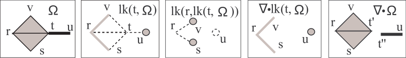
Figure 8.7: Examples of the decomposition process for the $2$-complex of Figure 4.4.

The decomposition of the $2$-complex (used in the running examples of Figures 4.4, 5.1 and many others. is depicted in Figure 8.7. From left to right, we summarize the step of the algorithm for vertex $t$, which is the only vertex that induces a split. First the link $lk({t},{\Omega})$ is computed, next the decomposition of the complex $lk({t},{\Omega})$ is attempted. We have that the link of $u$ in the complex ${lk({t},{\Omega})}$ is the empty set (i.e. $lk({u},{lk({t},{\Omega})})=\emptyset$). Thus, vertex $u$ is left unchanged in $\nabla\cdot{lk({t},{\Omega})}$. The link of $r$ in the complex ${lk({t},{\Omega})}$ is a $0$-complex containing the two vertices $u$ an $v$. Thus, the algorithm does not split vertex $r$ in $lk({t},{\Omega})$. Therefore, we obtain that $\nabla\cdot{lk({t},{\Omega})}={lk({t},{\Omega})}$. The complex $\nabla\cdot{lk({t},{\Omega})}$ it consists of two connected components. Therefore, the algorithm splits $t$ into two copies $t^{\prime}$ and $t^{\prime\prime}$, and this yields the decomposition in the rightmost frame. Next, for vertex $r$, we must consider $\nabla\cdot{lk({r},{\Omega})}$ (not shown in Figure 8.7). It is easy to see that $\nabla\cdot{lk({r},{\Omega})}={lk({r},{\Omega})}$. The complex ${lk({r},{\Omega})}$ has just one connected component and thus the algorithm do not split $r$. The same happens for the other vertices (i.e. $s$,$u$ and $v$) that do not split. Thus, the final $\nabla\cdot{\Omega}$ is the one depicted in the rightmost frame.

It is easy to prove that the Algorithm 8.5.1 has a time complexity that is slightly superlinear in the size of output.

Property 8.5.2.

The computation of  ${\rm DECOMPOSE}(\Omega,d)$ can be done in $O({d!}\cdot(NT\log{NT}))$ where $NT$ is the number of top simplices in the $d$-complex $\Omega$.

Proof 8.5.3.

It can be seen that all operations, but the computation of connected components and the decomposition of the link $LK$ can be done in $O(d\cdot NT\log{NT})$ . We start this analysis proving this fact. To prove this we recall that we have assumed that vertices and top simplices are coded as integers and that the complex $\Omega$ is presented in input as a $TV$ map between (indexes for) top simplex and $(d+1)$ array of vertices. The array will be padded with default values for non maximal top simplices. With these assumptions, it is easy to see that all operations, but the computation of connected components and the decomposition of $LK$ can be done in $O(d\cdot NT\log{NT})$.

We assume a standard implementation for the $TV$ map, for instance through a binary search tree. It is known that insertion and deletion in such $TV$ map can be done in logarithmic time vs. the size of the map [9]. Thus, the copy operation $1$ can be done with $NT$ reads and $NT$ writes into a map and this costs $\Theta(NT\log{NT})$ for each read we copy a $(d+1)$ array of Vertices and all these copies costs $\Theta((d+1)t)$. Thus operation $1$ takes $O(d\cdot NT\log{NT})$.

To deal with operations $4$,$5$ and $6$ we assume that, in an initialization phase, omitted in the abstract version of the algorithm, with time complexity of order $\Theta(NV\log{NV})$, where $NV$ is the number of vertices in $\nabla\cdot{\Omega}$, we can generate a $VT$ map where, for each vertex $v$, we store the simplex indexes for top simplices in $star({v},{\Omega})$. Being $NV\leq(d+1)NT$ we have that $\Theta(NV\log{NV})$ is $O(d\cdot NT\log{NT})$.

Then, for a given vertex $v$, we can build the $TV$ map for the representation for $lk(v)$. This can be done with just one access to the $VT$ map (costing $\Theta(\log{NV})$ and $O(log{NT})$) and $NT_{v}$ access to the $TV$ being $NT_{v}$ the number of top simplices in $lk(v)$ each costing $\Theta(\log{NT})$. For each access we copy up to $(d+1)$-Vertices and find the real dimension of the link. Thus for vertex $v$ for $5$ and $6$ we spend $O(log{NT})+\Theta(NT_{v}\log{NT})+\Theta(NT_{v}(d+1))$ that is $O(NT_{v}\log{NT})$. Thus we can provide a $TV$ representation for all links in $O(NT\log{NT})$. Thus we can extract in $4$ one after another Vertices in $\Omega$ in $\Theta(1)$ and all steps $5$ and $6$ takes $O(NT\log{NT}))$.

We note that size of a set and sequential access to all its elements can be done in $\Theta(1)$ and thus we perform $8$ in constant time once for each vertex for an overall cost of $\Theta(NV)$ and $O(d\cdot NT)$.

Sequential access to the element in $L$ and the creation of the new vertex can be done in constant time and all the repetitions of operations in $9$ and $10$ accounts for a time that is $\Theta(NC)$ where $NC$ is the number of vertex copies introduced by the decomposition process. Obviously we cannot have more vertex copies than the number of Vertices in the totally exploded version of $\Omega$ and thus $NC\leq(d+1)NT$. This proves that also $9$ and $10$ can be done in $O(d\cdot NT)$.

Finally step $11$ recalls for the editing of the $TV$ map encoding $\Omega_{c}$. Reasoning as for step $5$ we have that, for a given vertex $v$, we can edit the $TV$ map for the representation for $star({v},{\Omega_{c}})$. Sequential access to the elements in the domain of the map $\Psi$ will give the indexes of the $NT_{v_{\Psi}}$ top simplices to be modified, being $NT_{v_{\Psi}}$ the number of top simplices in $\Psi$. For each simplex we pay $NT_{v_{\Psi}}$ access to the $TV$ each costing $\Theta(\log{NT})$. For each a access we compare up to $(d+1)$-Vertices and find the entries to be modified. If $NT_{v}$ is the number of top simplices in $star({v},{\Omega_{c}})$ for step $11$ we spend $\Theta(NT_{v}\log{NT})+\Theta(NT_{v}(d+1))$ that is $O(NT_{v}\log{NT})$ to process a single vertex. Since summing all $NT_{v}$ for all Vertices yields at most $(d+1)NT$ we have that we can edit the $TV$ representation for all vertices in $O(d\cdot NT\log{NT})$.

This proves that all operations, but $7$ and $16$ can be done in $O(d\cdot NT\log{NT})$.

The subdivision of a complex into connected components (i.e., the ${\rm CONNECTED\_COMPONENTS}(\Omega_{c})$ call in line $16$) can be performed as the computation of connected components in a graph with $(d+1)NT$ arcs and $NT+NV^{\prime}$ nodes, where $NV^{\prime}$ is the number of vertices in $\nabla\cdot{\Omega}$ (note that $NV^{\prime}\leq(d+1)NT$). This is known (see [3]) to take $\Theta(d\cdot NT+NV^{\prime})$ and thus less than $O(d\cdot NT)$.

Thus, if we denote with $T^{d}(NT)$ the order of time complexity for the computation of ${\rm DECOMPOSE}(\Omega,d)$ we have that

$$T^{d}(NT)=O(d\cdot NT\log{NT})+\sum_{v\in V}{T^{(d-1)}(NT_{lk(v)})}$$

where: $V$ is the set of vertices in $\Omega$, and $NT_{lk(v)}$ is the number of top simplices in $lk(v)$. We can rewrite this recurrence using the trial solution $T^{d}(NT)=O({d!}\cdot NT\log{NT})$. With some standard algebra and using the fact that $\sum_{v\in V}{NT_{lk(v)}}\leq(d+1)NT$ we have the thesis.

Chapter 9 Non-Manifold Modeling Through Decomposition

9.1 Introduction

In this chapter, we consider the problem of describing a non-manifold object through its decomposition. Based on the theoretical framework from Chapter 8 we design a two-level data structure for non-manifold simplicial complexes in arbitrary dimension. In such a structure, each decomposition  component is represented through a topological data structure, while the connectivity relation among components is represented in a second layer describing how to stitch components at non-manifold joints. The resulting data structure is scalable since all information about non-manifold features for an object are represented in the upper-layer which becomes void in the manifold case. Moreover, the data structure is space-efficient and allows navigating in a non-manifold $d$-complex. In this chapter, we show that we are able to answer queries on adjacency and incidence relations efficiently. Please note that from now on we will switch from $d$ to $h$ for the letter used to give the dimension of the complex. This is to stress that, in the applications we have in mind, the dimension is something known and fixed. Even if we have developed many dimension independent results (i.e. for any $h$) still we do not expect to see applications that uses these results and one day are used for $h=2$ (i.e. surfaces) and the next day turn to handle volumetric data i.e. $h=3$. On the other hand, previous material was application independent.

This chapter is organized as a self contained unit. Therefore, in Section 9.2, we introduce some background notions that are used just in this chapter. In particular there is a quite lengthy section on face number relations that will be used to assess complexity of our data structure. The reader not interested in technical details of the proofs is advised to skip this. Next, in Section 9.3, we introduce basic supporting data structures, like: lists, sets etc., that will be used for the development of our algorithms and for the definition of the two layer data structure.

After these two background sections, in Section 9.4, we will introduce the data structure that will be used to encode the decomposition components. This data structure is defined and analyzed in this section. In particular we give algorithms to build and traverse a decomposition component and evaluate time and space requirements for these tasks.

Next, in Section 9.5 we introduce the second layer data structure. In particular, in Section 9.5.2, we will introduce a data structure to encode, in a unique framework, all the components of the decomposition. $\nabla\cdot{\Omega}$.

In Sections 9.5.3 and 9.5.4 we introduce data structures used to encode non-manifold features. This is the second layer of our data structure for non-manifolds. We give algorithms to build this second layer and we evaluate the time needed to build this data structure from the output of the decomposition algorithm. In the second part of this section we develop algorithms to extract topological relations in the original complex $\Omega$.

In section 9.5.4 we resume the definitions for the two layer data structure and present global formulas that gives time and space requirements of our two layer data structure. Next we compare these requirements against time and space requirements of most relevant proposals for non-manifold modeling.

9.2 Background

In this section we report some background notions that are necessary for the development of this chapter. In particular in sub-section 9.2.1, we introduce basic notations for topological relations. In sub-section 9.2.2 we report known results on the number of faces in particular simplicial complexes.

9.2.1 Topological Relations

In the following we will evaluate the effectiveness of our two layers representation by considering the complexity for retrieval of basic topological relations between simplices. Therefore we first introduce basic notations for topological relations we want to compute. Next we will introduce some standard naming used in modeling for certain topological relations that are usually called the TV,VT and TT relations.

The $S_{{nm}}$ relation

For a given $n$-simplex $\gamma\in\Omega$ in a $h$-complex $\Omega$, for any $n<m\leq h$, we will define the retrieval function $S_{{nm}}(\gamma)$ as the intersection between the star of $\gamma$ and the the set of simplices of order $m$ of $\Omega$ i.e. $S_{{nm}}(\gamma)=\star{\gamma}\cap\Omega^{[m]}$ (we recall that $\Omega^{[m]}$ denotes the set of simplices of $\Omega$ of order $m$). We can extend the definition of $S_{{nm}}(\gamma)$ to the case $n>m$ as $S_{{nm}}(\gamma)=2^{\gamma}\cap\Omega^{[m]}$ where $2^{\gamma}$ denotes the set of parts of $\gamma$. Finally we will define for $n>0$ the set $S_{{nn}}(\gamma)$ as the set of $n$-simplices in $\Omega$ that are $(n-1)$-adjacent to $\gamma$. For $n=0$ we will define $S_{{00}}(v)$ as the set of vertices $w$ s.t. $\{v,w\}$ is a simplex of $\Omega$. Both sets $S_{{nn}}$ and $S_{{00}}$ can be defined using sets $S_{{nm}}$ for $n<m$ being:

$$S_{{00}}(v) = \cup_{e\in S_{{01}}(v)}\{e-\{v\}\}$$ (9.1)

$$S_{{nn}}(\gamma) = \cup_{v\in\gamma}{S_{{(n-1)n}}(\gamma-\{v\})}$$ (9.2)

When needed we will emphasize the fact that the face relation is relative to a certain complex $\Omega$ by writing $S_{{nm}}(\gamma)$ as $S_{{nm}}(\gamma,\Omega)$. We note that the set union in formula 9.2 is a union between disjoint sets. Thus, the computation of $S_{{nn}}(\gamma)$ requires the computation of $S_{{(n-1)n}}(\gamma-\{v\})$ for all $v\in\gamma$. Similarly, all edges of the form $\{e-\{v\}\}$ in formula 9.1 are distinct. Thus, the computation of $S_{{00}}(v)$ reduces to the computation of $S_{{01}}(v)$. In the following we will assume that $S_{{nn}}$, for $n\geq 0$, is computed using formulas 9.1 and 9.2. Therefore, we do not exhibit a specific algorithm for the computation of $S_{{nn}}$. According to this assumption the time complexity for the computation of $S_{{00}}(v)$ will be the time complexity for the computation of $S_{{01}}(v)$. Similarly, the time complexity for the computation of $S_{{nn}}(\gamma)$ will be the sum of the time complexity for the computation of all $S_{{(n-1)n}}(\gamma-\{v\})$ for all $v\in\gamma$.

Finally we note that for $n>m$ the computation of $S_{{nm}}(\gamma)$ is obvious since it reduces to the generation of all subsets of $\gamma$ with $m$ elements. Thus in the following we will only consider the computation of $S_{{nm}}$ for $n\leq m$. For $n\neq m$ the set $S_{{nm}}(\gamma)$ is the set of $m$-simplices that are in a incidence relation with $\gamma$ (see Section 3.2.2). Therefore the set $S_{{nm}}$ is usually called a relation. In particular relation $S_{{nm}}$ is called a boundary relation if $n>m$ a co-boundary relation if $n<m$ and an adjacency relation if $n=m$ Boundary and coboundary relations toghether are called incidence relations. As already noted above, in the following we will only consider those relation we called coboundary relations.

The TV. VT and TT relations

All topological relations between simplices in an abstract simplicial complex are captured by the set of $S_{{nm}}$ relations. Nevertheless, a few alternative relations can be defined, In particular we will consider TV, VT and TT relations. The TV relation, probably, is the most elementary representation for an abstract simplicial complex.

For an abstract simplicial complex $\Omega$ the most obvious representation is given by the triple $(V,\Theta,\sigma_{0})$ where: $V$ is the set of vertices in $\Omega$; $\Theta$ is the set of top simplices in $\Omega$ (considered here as atomic objects) and $\sigma_{0}$ is the function ${\sigma_{0}}:{\Theta}\rightarrow{2^{V}}$, with $2^{V}$ being the set of parts of $V$.

The function $\sigma_{0}$ is usually referred to as the TV-relation. Similarly the triple $(V,\Theta,\sigma_{0})$ will be referred to as the $TV$ representation. A TV representation $(V,\Theta,\sigma_{0})$ defines the simplicial complex with vertices in $V$ given by the set of simplices $\cup_{\theta\in\Theta}\{\sigma_{0}(\theta)\}$. Two TV representations are equivalent if there are bijections between respective $V$s and $\Theta$s that commutes with $\sigma_{0}$. It is easy to see that equivalent TV representations defines isomorphic simplicial complexes. The function $\sigma_{0}$ can be defined in term of the previously defined topologic relations as $\sigma_{0}(t)=S_{{h0}}(t)$, where $h$ is the dimension of $t$.

A dual representation is the VT representation given by the triple $(V,\Theta,\sigma_{t})$ where $\sigma_{t}$ is the function ${\sigma_{t}}:{V}\rightarrow{2^{\Theta}}$ such that $\sigma_{t}(v)$ is given by the set of top simplices (of any dimension) incident in $v$. Thus we have $\sigma_{t}(v)=\cup_{0\leq h\leq d}S_{{0h}}(v)$. It is easy to see that $\sigma_{0}(t)=\{v|t\in\sigma_{t}(v)\}$. Since we can derive a TV representation from a VT representation, we have that the VT representation is unique up to isomorphism and is non-ambiguous, too.

For a regular abstract simplicial $h$-complex $\Omega$ we can define another topological relation we called the TT relation. We define the TT relation ${\mathcal{A}}$ as the relation ${\mathcal{A}}\subset\Theta^{2}$ defined by the condition: $\theta_{1}{\mathcal{A}}\theta_{2}$ iff $\theta_{1}$ and $\theta_{2}$ are adjacent. Note that relation ${\mathcal{A}}$ is always symmetric. For a given regular $d$-complex $\Omega$ its TT relation is uniquely defined. Unfortunately given a TT relation ${{\mathcal{A}}}$ there is not a unique regular $d$-complex whose TT relation is ${{\mathcal{A}}}$. This is true for any $d\geq 2$.

9.2.2 Face number relations

We define the $m$-th face number for an abstract simplicial complex $\Omega$ (denoted by $f_{m}(\Omega)$ or $f_{m}$) as the number of $m$-simplices in $\Omega$ i.e. $f_{m}(\Omega)={|\Omega^{[m]}|}$. (see Section 3.2 for the definition of $\Omega^{[m]}$). In this section we report some results for face numbers in arbitrary dimension. These are probably not relevant per se but they will be used to assess complexity of algorithms in the forthcoming sections. Many theorems gives relations between face numbers being the Kruskal-Katona theorem the most known result in this field (see [17] for a survey). We start recalling some simple relations for face numbers in manifold surfaces.

Manifold Surfaces

For a closed manifold surface $\Omega$ we have

$$\frac{3}{2}f_{2}(\Omega)=f_{1}(\Omega)$$ (9.3)

while, for a connected manifold surface with boundary, we have that:

$${3}f_{2}(\Omega)\leq 2f_{1}(\Omega)-3$$ (9.4)

Simplicial $h$-complexes embeddable in ${\rm I\kern-1.99997ptR}^{h}$

Next we will show that there are linear inequalities between face numbers $f_{h}$, $f_{h-1}$ and $f_{h-2}$ in the star of a vertex of an $h$-complex that can be geometrically embedded into ${\rm I\kern-1.99997ptR}^{h}$ as a compact geometric simplicial complex.

Property 9.2.1.

Let $\Omega$ be an $h$-complex geometrically embeddable into ${\rm I\kern-1.99997ptR}^{h}$ then $(h+1)f_{h}=2f_{h-1}$ for closed complexes and $(h+1)f_{h}\leq 2f_{h-1}-(h+1)$ for complexes with non empty boundary.

Proof 9.2.1.

To prove this property we proceed as follows. Let $\Gamma\in\Delta(\Omega)$ be an embedding of $\Omega$. We first show that at most two geometric $h$-simplices in $\Gamma$ can share a geometric $(h-1)$-face. The proof can be done by contradiction assuming that three geometric $h$-simplices $\theta_{1}$, $\theta_{2}$ and $\theta_{3}$ share an $(h-1)$-simplex $\gamma$. In this case the supporting hyperplane for $\gamma$ divides ${\rm I\kern-1.99997ptR}^{h}$ in two disjoint half-spaces. If we assume that $\theta_{1}$ and $\theta_{2}$ fall in the same half-space then these two geometric simplices must share interior points and this is not allowed in a geometric simplicial complex. Thus we have $(h+1)f_{h}=2f_{h-1}$ for closed complexes and $(h+1)f_{h}\leq 2f_{h-1}-(h+1)$ for complexes with non empty boundary. This is because the smallest boundary has (h+1) (h-1)-simplices. This completes the proof.

Next we show that, in general, for $h\geq 3$ there is a linear inequality between face numbers $f_{h}(star({\gamma},{\Omega}))$ and $f_{h-2}(star({\gamma},{\Omega}))$ in the open star of a $(h-3)$-simplex $\gamma$. This holds for whenever the simplicial complex $\Omega$ can be imbedded into ${\rm I\kern-1.99997ptR}^{h}$ as compact simplicial complex

Property 9.2.2.

For $h\geq 3$ let $\Omega$ be a regular $h$-complex geometrically embeddable into ${\rm I\kern-1.99997ptR}^{h}$ as a compact geometric simplicial complex and let $\gamma$ be an $(h-3)$-simplex in $\Omega$. In this situation the link of $lk({\gamma},{\Omega})$ is a triangulation embeddable in the $2$-sphere and, for the open star of $\gamma$ (i.e. $star({\gamma},{\Omega})$), we have $f_{h}(star({\gamma},{\Omega}))\leq 2(f_{h-2}(star({\gamma},{\Omega}))-2)$.

Proof 9.2.2.

We first note that, in a regular $h$-complex, the link of an $(h-3)$-simplex is a regular $2$-complex. We simply have to prove that we can imbed $lk({\gamma},{\Omega})$ in a $2$-sphere. Let $\Gamma$ be a geometric simplicial complex in ${\rm I\kern-1.99997ptR}^{h}$ that is the compact geometric realization of $\Omega$. This exists by hypothesis. It is easy to see that a geometric realization of the closed star ${\overline{star({\gamma},{\Omega})}}$ can be a compact geometric simplicial subcomplex of $\Gamma$. Let us call $S$ this subcomplex. Obviously $S$ is embeddable in ${\rm I\kern-1.99997ptR}^{h}$ and its boundary $\partial S$ is a geometric realization for $lk({\gamma},{\Omega})$.

With this situation in mind we first treat the case for $h=3$. In this case the geometric realization of the $(h-3)$-simplex $\gamma$ must be a single geometric vertex. Let $P_{0}$ be this point. It is easy to see that we can find a radius $r$ such that the complex $S$ fall outside the 2-sphere $\Sigma$ of radius $r$ centered in $P_{0}$. (i.e. ${\|{P-P_{0}}\|}>r$ for all $P\in\partial S$). It is easy to see that we can map geometric vertex $P\in\partial S$ onto the $2$-sphere $\Sigma$ through the continuous mapping $P\mapsto P_{0}+(P-P_{0})/{{\|{P-P_{0}}\|}}$. This mapping, restricted to $\partial S$, is invertible with continuous inverse. This proves that $\Sigma$ and $\partial S$ are homeomorphic and thus for $h=3$ we have proved that we can imbed $lk({\gamma},{\Omega})$ in a $2$-sphere.

For $h>3$ let $\{P_{0},\ldots,P_{h-3}\}$ the geometric simplex that is the geometric realization of $\gamma$ in ${\rm I\kern-1.99997ptR}^{h}$. Geometric Vertices $\{P_{0},\ldots,P_{h-3}\}$ must be affinely independent. This implies that in the euclidean vector space ${\rm I\kern-1.99997ptR}^{h}$ (see [72] Chapter 4 for basic definitions in Linear Algebra) the $(h-3)$ vectors $\{(P_{i}-P_{0})|i=1,\ldots,(h-3)\}$ are linearly independent and they generate a $(h-3)$-dimensional subspace of ${\rm I\kern-1.99997ptR}^{h}$. Let $W^{\gamma}$ be this subspace and let $W^{\gamma}_{\bot}$ the $3$-dimensional space such that the direct sum ${W^{\gamma}}\oplus{W^{\gamma}_{\bot}}$ gives ${\rm I\kern-1.99997ptR}^{h}$ (see for instance Ex. 5.49 [72]). Next we consider the abstract simplicial map $g$ that maps all and alone the Vertices of $\gamma$ into a single vertex $v$. This abstract simplicial map induces a geometric simplicial map defined as $|g|=[P_{i}\mapsto P_{0}|i=1,h-3]$ between $\Gamma$ and the geometric realization of $g(\Omega)$. In particular we have that $|g|(S)$ must be the geometric realization of $g({\overline{star({\gamma},{\Omega})}})$. Since $g(\gamma)=\{v\}$ we have that $g({\overline{star({\gamma},{\Omega})}})$ is the cone from $v$ to $lk({\gamma},{\Omega})$. Next we note that $|g|({W^{\gamma}})=\{0\}$ and $|g|({W^{\gamma}_{\bot}})={W^{\gamma}_{\bot}}$. Thus we have that $|g|({\rm I\kern-1.99997ptR}^{h})={W^{\gamma}_{\bot}}$ and therefore ${W^{\gamma}_{\bot}}$ must include $|g|(S)$. Thus we have a geometric realization for the cone from $v$ to $lk({\gamma},{\Omega})$ in the euclidean subspace ${W^{\gamma}_{\bot}}$. This is a $3$-dimensional subspace of ${\rm I\kern-1.99997ptR}^{h}$. Thus we have a geometric realization for the cone from $v$ to $lk({\gamma},{\Omega})$ in ${\rm I\kern-1.99997ptR}^{3}$. Reasoning as in the case for $h=3$ we prove that $lk({\gamma},{\Omega})$ can be embedded in a $2$-sphere. This proves the first part of the thesis.

The second part comes easily from the Euler formula. We have just proven that the link of each $(h-3)$-simplex $\gamma$ is a triangulation that can be imbedded in a $2$-sphere. If the link is homeomorphic to the $2$-sphere we have $f_{2}-f_{1}+f_{0}=2$ and $3f_{2}=2f_{1}$. This yields $f_{2}=2(f_{0}-2)$. When the link is not homeomorphic to the $2$-sphere we can write $f^{k}_{2}-f^{k}_{1}+f^{k}_{0}=1$ and $\frac{3}{2}f^{k}_{2}\leq f^{k}_{1}-1$ being $f^{k}_{i}$ the face numbers for the $k$-th connected component of the link. This yields $f^{k}_{2}\leq 2(f^{k}_{0}-2)$ in the $k$-connected connected component of the link. Summing over the $c$ different connected components of the link we get $f_{2}\leq 2(f_{0}-2c)$. Thus we can write $f_{2}\leq 2(f_{0}-2c)\leq 2(f_{0}-2)$. . Now we note that to a $j$-face in $lk({\gamma},{\Omega})$ correspond a $h-2+j$ face in the open star $star({\gamma},{\Omega})$ and thus we rewrite the previous formula for $lk({\gamma},{\Omega})$ as $f_{h}(star({\gamma},{\Omega}))\leq 2(f_{h-2}(star({\gamma},{\Omega}))-2)$. This completes the proof.

Note that summing all over the $(h-3)$ simplices in a manifold $h$-abstract simplicial complex  $\Omega$ we have the following property:

Property 9.2.3.

Let $\Omega$ a closed manifold $h$-complex imbeddable in ${\rm I\kern-1.99997ptR}^{h}$ in this situation

$${{h+1\choose h-2}}f_{h}(\Omega)-{{h\choose h-2}}f_{h-1}(\Omega)+{{h-1\choose h-2}}f_{h-2}(\Omega)=2f_{h-3}$$

Proof 9.2.3.

In a closed $h$-manifold complex $\Omega$ we have every link $lk({\gamma},{\Omega})$ of an $(h-3)$-simplex $\gamma$ is homeomorphic to a sphere and by Euler formula applied to that link we have $f_{2}-f_{1}+f_{0}=2$. Now there are, respectively, a 2-simplex or a 1-simplex or a 0-simplex in $lk({\gamma},{\Omega})$ for, respectively, every top $h$-simplex or $(h-1)$-simplex or $(h-2)$-simplex in $star({\gamma},{\Omega})$, because $\gamma$ is a $(h-3)$-simplex. Thus summing the relation $f_{2}-f_{1}+f_{0}=2$ all over the links of all $(h-3)$ simplices in a manifold abstract simplicial complex  $\Omega$ we mention each top simplex in $\Omega$ once for each $h-3$ face it has. Thus summing $f_{2}-f_{1}+f_{0}=2$ all over the complex we obtain something like $\ldots=2f_{h-3}$. Let us see what to put instead of dots. On the other hand an $h$-simplex $\theta_{h}$ is mentioned in this sum as many times as $\theta_{h}$ enters in a star of some of its $(h-3)$-faces. Thus we have to count the number of $(h-3)$-faces of $\theta_{h}$ and put this to multiply $f_{h}$. The number of $h-3$ faces of an $h$-simplex is given by a choice od $h-2$ vertices among its $h+1$ vertices. So an $h$ face is mentioned ${{h+1\choose h-2}}$ times. Thus summing $f_{2}-f_{1}+f_{0}=2$ all over the complex we obtain something like ${{h+1\choose h-2}}f_{h}+\ldots=2f_{h-3}$. Similarly an $(h-1)$-simplex $\theta_{h-1}$ is mentioned in this sum as many times as $\theta_{h-1}$ enters in a star of some of its $(h-3)$-faces. Thus we have to count the number of $(h-3)$-faces of $\theta_{h-1}$ and put this to multiply $f_{h-1}$. The number of $h-3$ faces of an ${h-1}$-simplex is given by a choice of $h-2$ vertices among its $h$ vertices. So an $h-1$ face is mentioned ${{h\choose h-2}}$ times. Thus summing $f_{2}-f_{1}+f_{0}=2$ all over the complex we obtain something like ${{h+1\choose h-2}}f_{h}-{{h\choose h-2}}f_{h-1}\ldots=2f_{h-3}$ Similarly we mention each $(h-2)$-simplex ${{h-1\choose h-2}}$ times. Thus we obtain the formula of the thesis.

Non-linear relations between $f_{4}$ and $f_{0}$ for stars in $4$-balls

In the following we will be interested in evaluating the complexity of traversal of our two layer data structure. This require some understanding of how face numbers are related in generic $h$-complexes. These notions will be specialized to initial quasi-manifolds. The results shows that, in higher dimension, complexity must be, at least, quadratic because the complexity of the structure of the complex could be quadratic, or more.

In the previous section we have found linear relations between face numbers $f_{h}$, $f_{h-1}$ and $f_{h-2}$ in the star of a vertex of an $h$-complex that can be geometrically embedded into ${\rm I\kern-1.99997ptR}^{h}$. For $4$-complexes this ensure a linear relation among $f_{4}$, $f_{3}$ and $f_{2}$. We note that, for $h=4$, the Properties 9.2.1 and 9.2.2 do not ensure a linear inequality between the face numbers $f_{4}$ and $f_{1}$. Similarly no linear relation could be found, in general, between face numbers $f_{4}$ and $f_{0}$. in the star of a vertex of a $4$-complex. In this sub-section we will study what happens to face numbers in stars of $4$-complexes while, in the following section, we will investigate face number relations for complexes that cannot be embedded in ${\rm I\kern-1.99997ptR}^{h}$.

In particular, we will exhibit a manifold $4$-complex $\Omega$ with a vertex $v$ s.t. $f_{4}(\overline{star({v},{\Omega})})=f_{0}(f_{0}-3)/2$ with $f_{0}=f_{0}(\overline{star({v},{\Omega})})$. Therefore complexity of this relation could be quadratic.

In fact it is possible to build a triangulation of the $4$-ball where there is at least a vertex $w$ for which $f_{4}(\overline{star({w},{\Omega})})=f_{0}(f_{0}-3)/2$ where $f_{0}=f_{0}(\overline{star({w},{\Omega})})$ is the number of vertices in $\overline{star({w},{\Omega})}$ that are distinct form $w$. To build such a complex we just have to take as $4$-complex the cone from an arbitrary vertex $w$ to the boundary of the Cyclic Polytope $C_{4}(f_{0})$. To show this fact we introduce polytopes.

Definition 9.2.4 (Polytope and Cyclic Polytope).

A $k$-polytope with $n$ Vertices (denoted as $\Pi(n)$) is the convex-hull of a set of $n$ points in ${\rm I\kern-1.99997ptR}^{k}$. The cyclic $k$-polytope with $n$-points (denoted by $C_{k}(n)$) is a polytope in ${\rm I\kern-1.99997ptR}^{k}$ that has the property of having the maximum face number $f_{i}$ for all $0\leq i<k$.

Following the conventions used in this thesis we denote with $f_{0}$ the number of points $n$ and therefore we will use $\Pi(f_{0})$ instead of $\Pi(n)$.

The cyclic $k$-polytope has the maximum face number $f_{i}$ for all $0\leq i<k$. Any other $k$-polytope has the face number $f_{i}$ smaller than the corresponding face number of the cyclic polytope. The so called Upper Bound Theorem by McMullen [84] gives a sets of formulas to compute these upper bounds for face numbers. (See [60] for an extension of this result to spheres and recently to homology manifolds [102] and [17] Pg. 298-300).

The explicit formula for the computation of all the face numbers $f_{i}$ of the cyclic polytope vertices is quite complex (See [41] Sections 4.7.3. and 9.6.1). We just report the specialization of this formula for $i=d-1$:

$$f_{d-1}={f_{0}-\left\lceil{d/2}\right\rceil\choose\left\lfloor{d/2}\right\rfloor}+{f_{0}-\left\lfloor{d/2}\right\rfloor-1\choose\left\lceil{d/2}\right\rceil-1}$$ (9.5)

In particular for $C_{4}(f_{0})$ we have $f_{3}=f_{0}(f_{0}-3)/2$ (simply put $d=4$ in equation 9.5). Since $C_{4}(f_{0})$ is a polytope we have that $\partial C_{4}(f_{0})$ is homeomorphic to the $3$-sphere. Thus, for all the classes of $3$-complexes that includes the $3$-sphere (e.g. manifolds, pseudomanifold, initial-quasi-manifold, etc.) we can say that there cannot be, in general, a linear relation between $f_{0}$ and $f_{3}$.

Property 9.2.4.

There exist a triangulation $TB^{4}$ of the $4$-ball imbeddable in ${\rm I\kern-1.99997ptR}^{4}$ and a vertex $w$ such that $f_{4}(\overline{star({w},{TB^{4}})})=f_{0}(f_{0}-3)/2$ with $f_{0}$ the number of vertices in $\overline{star({w},{TB^{4}})}$ distinct from $w$.

Proof 9.2.5.

We take as $TB^{4}$ the cone from $w$ to the boundary of the cyclic $4$-polytope $C_{4}(f_{0})$. Thus taking the cone from $w$ to a tetrahedron in the boundary of $C_{4}(f_{0})$ we obtain a $4$-simplex in $\overline{star({w},{TB^{4}})}$. Thus, $f_{4}(\overline{star({w},{TB^{4}})})$ is the number of tetrahedra in the boundary of $C_{4}(f_{0})$, This number is given by $f_{3}=f_{0}(f_{0}-3)/2$ where $f_{0}$ is the number of vertices in $\overline{star({w},{TB^{4}})}$ distinct from $w$.

Now we just have to prove that what we called $TB^{4}$ is a triangulation of the $4$-ball. To take this cone we just have to take $w$ not in $C_{4}(f_{0})$. Since all $3$-spheres are combinatorially equivalent [94] we can also say that $\partial C_{4}(f_{0})$ is a triangulation of the $3$-sphere embedded in ${\rm I\kern-1.99997ptR}^{4}$ that is a combinatorial manifold. Thus, by Property 3.5.3, the cone $TB^{4}$ from $w$ to $\partial C_{4}(f_{0})$ is a triangulation of the $4$-ball as a combinatorial manifold. If we choose the geometric realization of $w$ within the the geometric realization of $C_{4}(f_{0})$ it is easy to see that the cone $TB^{4}$ admits a geometric realization in ${\rm I\kern-1.99997ptR}^{4}$.

The above Property generalize to $d$-balls showing that the number of top simplices in a vertex star can become quite large.

Property 9.2.5.

There exist a triangulation $TB^{d}$ of the $d$-ball embeddable in ${\rm I\kern-1.99997ptR}^{d}$ such that, for a certain vertex $w$ in $TB^{d}$, $f_{d}(\overline{star({w},{TB^{d}})})=\Theta(f_{0}^{\left\lfloor{d/2}\right\rfloor})$ with $f_{0}$ is the number of vertices in $\overline{star({w},{TB^{d}})}$.

Proof 9.2.6.

Using the explicit formula for face numbers in cyclic polytopes ${C_{d}(f_{0})}$ (see Formula 9.5) and the approximation suggested by the Stirling formula

$$\lim_{n\rightarrow\infty}{\frac{{n!}}{n^{n}e^{-n}\sqrt{2\pi\ n}}}=1$$

(see, for instance, [75] §21.4-2) one easily shows that the number of top simplices in the cyclic polytope ${C_{d}(f_{0})}$ is given by $f_{d-1}=\Theta(f_{0}^{\left\lfloor{d/2}\right\rfloor})$ (see 9.2.3 for the definition of the complexity order $\Theta(n)$). Therefore, with arguments similar to those used in the proof of Property 9.2.4, one builds $TB^{d}$ by selecting a vertex $w$ within the geometric realization of ${C_{d}(f_{0})}$ in ${\rm I\kern-1.99997ptR}^{d}$ and then takes the cone from $w$ to $\partial C_{d}(f_{0})$. The polytope ${C_{d}(f_{0})}$ has a boundary that is a combinatorial $(d-1)$-sphere. Thus, the resulting cone is a triangulation of the combinatorial $d$-ball embeddable in ${\rm I\kern-1.99997ptR}^{d}$. Considering the star of vertex $w$ we have $f_{d}(\overline{star({w},{TB^{d}})})=\Theta(f_{0}^{\left\lfloor{d/2}\right\rfloor})$ with $f_{0}$ the number of vertices in $\overline{star({w},{TB^{d}})}$. In fact a $d$-simplex in this star correspond to a $(d-1)$-simplex in the cyclic polytope ${C_{d}(f_{0})}$.

Following the ideas in the proofs above it is easy to build a $d$-ball $TB^{d}$, for $d$ sufficiently high, in which there exist an $n$-simplex $\gamma$ for which $f_{d}(\overline{star({\gamma},{TB^{d}})})=f_{3}=f_{0}(f_{0}-3)/2$ with $f_{0}$ the number of vertices in $\overline{star({\gamma},{TB^{d}})}$ that are not in $\gamma$ . The property below gives a formal statement of this fact.

Property 9.2.6.

For any natural $n\geq 0$, there exist a combinatorial $d$-ball $TB^{d}$ that can be embedded in ${\rm I\kern-1.99997ptR}^{d}$, for $d=4+n$, and an $n$-simplex $\gamma$ such that $f_{d}(\overline{star({\gamma},{TB^{d}})})=f_{3}=f_{0}(f_{0}-3)/2$ with $f_{0}$ the number of vertices in $\overline{star({\gamma},{TB^{d}})}$ that are not in $\gamma$.

Proof 9.2.7.

To build such a triangulation of $B^{d}$ we consider objects in the euclidean space ${\rm I\kern-1.99997ptR}^{d}$ for $d=n+4$. We first take the geometric realization of the cyclic polytope ${{C_{4}(f_{0})}}$ in ${\rm I\kern-1.99997ptR}^{d}$. Next we take a geometric realization of the standard $n$-simplex $\gamma$ in ${\rm I\kern-1.99997ptR}^{d}$ that fits in the interior of the geometric realization of the cyclic polytope ${{C_{4}(f_{0})}}$. Then, the complex $TB^{d}$ is obtained as the cone from $\gamma$ to ${\partial C_{4}(f_{0})}$. We have that ${\partial C_{4}(f_{0})}$ is combinatorially equivalent to the $3$-sphere and thus the cone from the $n$-simplex $\gamma$ to the boundary ${\partial C_{4}(f_{0})}$ is combinatorially equivalent to the $d$-ball with $d=n+3+1$ (See Property 3.5.3). The complex $TB^{d}$ is realizable in ${\rm I\kern-1.99997ptR}^{d}$ and is a triangulation of the $d$-ball as a combinatorial manifold.

Thus, also the number of top simplices in an $n$-simplex star might become extremely large in a $d$-complex in higer dimension. The above property refers to the case $d=n+4$. However, combining the proof above and that of Property 9.2.5 it is easy to build an $h$-complex $TB^{h}$, for $h$ sufficiently high, in which there exist a $n$-simplex $\gamma$ for which $f_{d}(\overline{star({\gamma},{TB^{d}})})=\Theta(f_{0}^{\left\lfloor{d/2}\right\rfloor})$ with $f_{0}$ is the number of vertices in $\overline{star({\gamma},{TB^{d}})}$.

Face numbers in stars of non embeddable $3$-manifolds

In the second part of this section we will study the influence of non embeddability on face numbers for $3$-complexes. We will find examples of $3$-complexes non-embeddable in ${\rm I\kern-1.99997ptR}^{3}$ that contains a vertex $v$ for which there is not a linear relation between $f_{3}(\overline{star({v},{\Omega})})$ and $f_{0}(\overline{star({v},{\Omega})})$.

The above properties shows that a quite large number of $(d-1)$-faces can fit in the boundary of a cyclic $d$-polytope as $d$ grows. This enables us to build $4$-balls where there is a vertex whose star has a number of top simplices that is non-linear w.r.t. the number of incident vertices. Therefore one might suspect that our requirement on embeddability in ${\rm I\kern-1.99997ptR}^{h}$ might be unnecessary when $h$ is low and that it is not possible to have $3$-complex where the number of tetrahedra in a vertex star in non-linear w.r.t. the number of vertices in the star its-self. This is not the case. In fact similar examples pops up already for in $3$-complexes if we drop the requirement on embeddability in ${\rm I\kern-1.99997ptR}^{3}$. Indeed if we allow (rather exotic) $3$-complexes where a vertex star might have a toroidal surface boundary we obtain quite large face numbers with quite few vertices. These complexes are neither $3$-balls not $3$-manifolds but they fall in the class of initial-quasi-manifold $3$-complexes.

This can be shown by providing a family of manifold surfaces $\Sigma(g)$, with genus $g$, for which do not exist a linear relation between $f_{0}$ and $f_{2}$. If such a family exists, then, with an argument similar to that used in the previous property, we can show that, in the cone from $w$ to $\Sigma(g)$, the number of tetrahedra in the star of $w$ is non-linear w.r.t. the number of vertices in this star.

Indeed the family of minimal triangulations of 2-manifolds provides the required family $\Sigma(g)$.

Property 9.2.7.

There exist countably many initial-quasi-manifold $3$-complexes $B(g)$, for any natural $g>0$, not embeddable in ${\rm I\kern-1.99997ptR}^{3}$, s.t. there exist a vertex $w$ for which $f_{3}(\overline{star({w},{B(g)})})=\Theta({f_{0}}^{2})$ with $f_{0}$ the number of vertices in $\overline{star({w},{B(g)})}$ that are distinct from $w$. In particular we have: ${{(f_{0}^{2}-3f_{0}+8)}/3}<f_{3}(\overline{star({w},{B(g)})})\leq{{f_{0}(f_{0}-1)}/3}$.

Proof 9.2.8.

It can be shown (see [65] Pg. 122) that in a class ${\mathcal{M}}$ of topologically equivalent $2$-manifolds there exist an abstract simplicial complex with a minimal number of triangles given by

$$f_{2}=2\left\lceil{\frac{7+\sqrt{49-24\chi(\mathcal{M})}}{2}}\right\rceil-2\chi(\mathcal{M})$$ (9.6)

where $\chi(\mathcal{M})$ is the common Euler characteristic for the class of homeomorphic surfaces ${\mathcal{M}}$. This holds for all $2$-manifolds minimal triangulation with the exception of the double torus $T_{2}$, of the Klein’s bottle and of the non orientable surface of genus $3$ whose minimal triangulation respectively takes 24, 16 and 20 triangles.

We now prove that, in this family of minimal triangulations of a $2$-manifold, the face number $f_{2}$ is $\Theta(f_{0}^{2})$. This can be proven using the definition of $\chi=f_{2}-f_{1}+f_{0}$ and the fact that, for closed $2$-manifolds, we have that $(3/2)f_{2}=f_{1}$, and thus $f_{0}-(1/2)f_{2}=\chi$. By rewriting $\chi$ in Equation 9.6 we get $f_{0}=\left\lceil{\frac{7+\sqrt{49-24\chi}}{2}}\right\rceil$ and therefore must be $f_{0}\geq{\frac{7+\sqrt{49-24\chi}}{2}}>f_{0}-1$. Solving $f_{0}\geq{\frac{7+\sqrt{49-24\chi}}{2}}$ with $\chi=f_{0}-(1/2)f_{2}$ we obtain $f_{2}\leq{f_{0}(f_{0}-1)}/3$. Solving ${\frac{7+\sqrt{49-24\chi}}{2}}>f_{0}-1$ we obtain $f_{2}>(f_{0}^{2}-3f_{0}+8)/3$ thus we get

$${{(f_{0}^{2}-3f_{0}+8)}/3}<f_{2}\leq{{f_{0}(f_{0}-1)}/3}$$ (9.7)

Thus, to complete the proof we just have to take the minimal triangulation $\Sigma(g)$ of the surface of genus $g$. We recall that for a closed orientable $2$-manifold ${\mathcal{M}}$ the genus $g$ is given by $\chi({\mathcal{M}})=2-2g$ while for closed non-orientable $2$-manifold we have $\chi({\mathcal{M}})=2-g$. In general we can write these two relations using the third Betti number $\beta_{2}$. We recall that $\beta_{2}$ is $0$ for non orientable surfaces and $1$ for orientable surfaces. With this definitions we can write $\chi({\mathcal{M}})=2-(1+\beta_{2})g$. The number of vertices in $\Sigma(g)$ can be obtained by reworking Equation 9.6 and using $\chi({\mathcal{M}})=2-(1+\beta_{2})g$ we get

$$f_{0}=\left\lceil{\frac{7+\sqrt{1+24(1+\beta_{2})g}}{2}}\right\rceil$$

Note that for $f_{0}>4$ we must have $g>0$. Taking the $3$-complex $B(g)$ as the cone from a new vertex $w$ to $\Sigma(g)$ and reasoning as in the proof of Property 9.2.4 we show that in $B(g)$ we have ${{(f_{0}^{2}-3f_{0}+8)}/3}<f_{3}(\overline{star({w},{B(g)})})\leq{{f_{0}(f_{0}-1)}/3}$ being $f_{0}$ the number of vertices in $\overline{star({w},{B(g)})}$ that are distinct from $w$. In particular we have: $f_{3}(\overline{star({w},{B(g)})})=\Theta({f_{0}}^{2})$.

To complete this proof we just have to show that $B(g)$ is an initial-quasi-manifold and that it cannot be embedded in ${\rm I\kern-1.99997ptR}^{3}$. It is easy to see that $lk({v},{B(g)})$ is homeomorphic to the $2$-ball for $v\neq w$ and for $w$ we know $lk({w},{B(g)})=\Sigma(g)$. Thus, for any vertex $v$ in $B(g)$ we have that $lk({v},{B(g)})$ is a $2$-manifold. Thus the link of each vertex is $2$-manifold-connected and, therefore, the star of each vertex is $3$-manifold-connected. Thus $B(g)$ must be an initial-quasi-manifold.

Finally non embeddability is proven by contradiction. Let us assume that $B(g)$ is embeddable in ${\rm I\kern-1.99997ptR}^{3}$. By Property 9.2.2 we have that $lk({w},{B(g)})=\Sigma(g)$ can be embedded in a $2$-sphere. Thus we can take a pole within a triangle of $\Sigma(g)$ and project, by stereographic projection, the $1$-skeleton of $\Sigma(g)$ as a planar graph. This graph has a number of faces that is one less the number of triangles of $\Sigma(g)$ (i.e. $f_{2}-1$). Using the Euler formula we get $1=(f_{2}-1)-f_{1}+f_{0}$. Thus we have that $\chi(\Sigma(g))=2$. This implies $g=0$, that, in general, is false.

9.2.3 Complexity

We recall briefly the standard notation for complexity. Let $T(n)$ be a function expressing the measure of a certain quantity $X$ w.r.t. a certain parameter $n$ (e.g. $T(n)$ could be the time spent for computation w.r.t. the size of the input $n$ or $T(n)$ could be the number of bits needed to store a certain triangulation w.r.t. the number of triangles, etc.). We will say that the quantity $X$ is in $\Theta(f(n))$ if and only if  there are three strictly positive constants $c_{1}$, $c_{2}$ and $n_{0}$ such that $c_{1}f(n)\leq T(n)\leq c_{2}f(n)$ for all $n>n_{0}$.

Similarly we will say that the quantity $X$ is in $O(f(n))$ if and only if  there are two strictly positive constants $c$ and $n_{0}$ such that $T(n)\leq cf(n)$ for all $n>n_{0}$.

Finally we recall we say that the quantity $X$ is in $\Omega(f(n))$ if and only if  there are two strictly positive constants $c$ and $n_{0}$ such that $cf(n)\leq T(n)$ for all $n>n_{0}$. Note that $X$ is in $\Theta(f(n))$ if and only if  $X$ is both in $O(f(n))$ and $\Omega(f(n))$.

9.3 Supporting Data Structures

9.3.1 Introduction

In this section we briefly introduce a number of classic data structures. For each data structure we will specify the primitives that will be used in this thesis to access the data structure, the sintax used to denote these primitives and the time complexity of the standard algorithm used to implement them. We will assume to have a pseudocode language for data type definitions that supports some type constructors we will introduce in the following.

9.3.2 Lists

In the following algorithms we assume to have a pseudocode language that supports data definitions through a set of type constructors. For lists we assume a type constructor of the form list of $T$, being $T$ a generic type that do not have to satisfy any particular constraint. We will denote with ${<\!\mbox{}\!\!>}$ the empty list. If $e$ is an object of type $T$ we will denote with ${<\!e\!\!>}$ the list made up of a single element. We assume to have an implementation for the usual operations on lists. In particular, if $l$ is an object of type list of $T$ we will have that $l.{\rm TOP}$ returns the first element in the list and $l.{\rm POP}$ returns a pointer to the list without the first element. We will use the notation ${<\!e\!\!>}+l$ to denote the list obtained appending $e$ at the beginning of the list $l$. We assume that all the above operations on lists can be done in constant time. For two objects $l_{1}$ and $l_{2}$ of list type we assume to have an operator $l_{1}+l_{2}$ to concatenate lists. This can be done in $\Theta(|l_{1}|)$.

We assume that is possible to have a method to retrieve, in constant time, one after one, all elements $v$ in a list $l$. Thus, we will use an expression of the form ”$v$ in $l$” as control predicate for loops. When list $l$ is used for such an iteration we assume that the list is not modified and we assume that there exists a method, denoted by $l.CircularNext$, that can be used to fetch the element after the one currently returned for the iteration. If the last element is currently returned for iteration then $l.CircularNext$ returns the first element in the list $l$. Obviously we expect to do this in constant time. Finally we assume to have an explicit type casting operation ${\bf list}(s)$ that convert a set $s$ into the list of its elements. This latter operation can be done in time proportional to the size of the output.

Lists will be used for local variables in algorithms and are not used within the topological data structure. Thus the space requirements for this data structure is not analyzed.

9.3.3 Bit and Bit Vectors

Next we assume to have the option to define vectors with a huge number of bits. In fact we will use bit vectors with one bit for each top simplex in the abstract simplicial complex under analysis. We assume that a fresh copy of the bit vector $\Theta$ is allocated by the declaration var $\Theta$: array $[Min,\ldots,Max]$ of bit. This creates $Max-Min+1$ bits initialized to zero. We assume to have three operations on bits. The three operations are: the operation ${\rm SET}$, that sets the bit; the operation ${\rm RESET}$, that resets the bit and the operation ${\rm TEST}$ that returns a boolean value that will be true if and only if  the bit is set. If $B$ is a bit we also use $B$ as a variable that can hold two values $0$ and $1$. Obviously we will say that the bit is set when it contains 1. Finally we assume that we can use bit vectors wherever a positive integer is needed. In this case we assume an implicit cast from bit vectors to positive integers. Bits and bit vectors will be used for temporary marking and are not used within the topological data structure. Thus the space requirements for this data structure are not analyzed.

9.3.4 Sets

We assume that in our language for data type declaration we can write: $\mbox{\bf set of }Domain$ being $Domain$ a data type whose values must form a totally ordered set. We do not assume anything else about sets elements. Thus the time complexity for sets and maps operations is given, in this section, by giving the number of comparisons between two elements in the $Domain$ set. To get the real time complexity for a particular set operation we must multiply the number of comparisons by the time complexity for a single comparison between two elements in $Domain$.

With this assumption about ordering of the type $Domain$ we have that sets can be implemented with binary search trees (BST) maintained as an AVL tree (see [96] Pg. 15-17 for a careful presentation of AVL tree primitives. See also [87] Ch. 4). Sets will be used for local variables in algorithm and are not used within the topologic data structure. Thus the space requirements for these AVL trees is not taken into account here.

We mention the fact that the set data structure is offered as an ”off the shelf” component in the STL (Standard Template Library) [105, 121] that is part of the C++ Standard Library and in the commercial library LEDA [6]. What will be the implementation technique used in these packages we have checked that the time complexity listed in this section are guaranteed by these implementations. In particular we report the time complexity guaranteed by the STL library and add the complexity provided by LEDA when this is different.

If $v$ is an object in set element $Domain$ and $S_{1}$ and $S_{2}$ are object of type $\mbox{\bf set of }Domain$ we assume that are legal expressions of set type $S_{1}\cup S_{2}$ and $S_{1}\cap S_{2}$. Both union and intersection can be done in STL with $O(|S_{1}|+|S_{1}|)$ comparisons between sets elements. In LEDA union takes $O(|S_{2}|\log{|S_{1}|+|S_{1}|})$ and intersection takes $O(|S_{1}|\log{|S_{1}|+|S_{1}|})$ comparisons.

Set membership, denoted by $v\in S$, can be tested in $O(\log{|S|})$ comparisons. We can compute the subset of element of $S_{1}$ that are not in $S_{2}$, denoted by $S_{1}-S_{2}$, with $O(|S_{2}|+|S_{1}|)$ comparisons. This complexity is offered by STL while LEDA uses a different algorithm that takes $O(|S_{2}|\log{|S_{1}|+|S_{1}|})$ comparisons.

We can test in STL whether set $S_{1}$ is included in $S_{2}$, a test denoted by $S_{1}\subset S_{2}$, with $O(|S_{1}|+|S_{2}|)$ comparisons. However we note that this can be done by testing all elements in $S_{1}$ and this takes $O(|S_{1}|\log{|S_{2}|})$. We can test whether a set $S$ is empty, a test denoted by $S=\emptyset$, in constant time. We have that all elements in a set can be provided in constant time and thus we assume that we can control loops with expressions of the form forall $t\in S$, with no extra time overhead.

Finally we recall that we already assumed that is possible to cast an object of set type into a list. Similarly we assume that it is possible to cast an array of $n$ distinct elements $T$ into a set denoted by ${\bf set}(T)$. This can be done in $\Theta(n\log{n})$.

9.3.5 Maps

The map data type offer a natural implementation for functions. In fact, maps, from an abstract point of view, are simply sets of couples, such that there are not two couples with the same first element. Implementation for maps can be obtained from implementation for sets simply adding extra space to hold the second element of the couple. For this reason we assume that maps can be implemented as a BST maintained as an AVL tree. This choice is adopted whenever maps are used for local variables within our algorithms.

However, we anticipate that maps are used in our topological data structure. In particular, maps are used in the second layer of our two layer data structure that encodes information about non-manifoldness. We will build these maps using a AVL tree and convert these maps into a more compact representation at the end of the construction phase. This compact version is obtained by transforming the AVL tree into a left complete binary tree or an heap (see [97] Pg. 41-48 and [32] Ch. 7-8 for an introduction to Heaps). It is well known that an heap can be stored into an array. This conversion can be done in linear time vs. the size of the domain of the map. The heap data structure still guarantees logarithmic time access and supports compact storage of these maps. In fact the space needed to encode the map as an heap is exactly the space needed to hold all the couples in the map.

We assume to have, in our pseudocode, the option to define maps with a type constructor of the form $\mbox{\bf map of }Domain\,\mbox{\bf into }Codomain$. The type $Domain$ must adhere the same requirements we detailed for sets. The type $Codomain$ need not to satisfy any particular requirement. Maps, being sets of couples, inherits all the primitives that we have presented for sets. In particular, in a map $M$, if we filter out the second element, we obtain the set denoted by $domain(M)$. This set is available, in constant time, as a set to control loops.

Maps adds an handy way to store and retrieve elements indexed by elements in the set $Domain$. If $M$ is a map and $d$ is an element in the set $domain(M)$ we will assume that $M[d]$ denotes the element in $Codomain$ such that $(d,M[d])\in M$. The element $M[d]$ can be obtained with $\Theta(\log{|domain(M)|})$ comparisons. Similarly, we assume that, in our pseudocode, we can associate an element $e$ in $Codomain$ to an element $d$ in the $Domain$ by an assignment of the form $M[d]\leftarrow e$. The execution of this assignment, excluding the time necessary to retrieve $e$, requires $\Theta(\log{|domain(M)|})$ comparisons.

Finally we note that maps that are present in the topological data structure are used only for retrieval and, once created, are not modified at all. Thus, the choice of an heap implementation for these maps is feasible. If mesh editing is required then a dynamic data structure is needed and we will have to use an AVL tree for the implementation of these maps. Obviously, this will result in heavier memory requirements. However we note that these requirements applies only to maps that will be used in the second layer dealing with the non-manifold structure of the complex. We recall that one of our main assumptions is that this structure must have a limited extension.

We mention again the fact that the map data structure, implemented with BST is offered as an ”off the shelf” component in STL from the C++ Standard Library. What LEDA calls maps is implemented using hashing and thus it is not suitable for our analysis. Howeve the LEDA data type called dictionary offer the right, tree based, data structure for maps. What will be the implementation technique used in these packages we have checked that operations listed here are offered by these packages with the time complexity listed in this section.

9.3.6 Hashed Sets

We will assume to have the option to define sets implemented with an hash table. Hash tables offers insertion and set membership test in average constant time. Such a set will be defined with a data type declaration of the form var H[n] hashed set of Domain. Where $n$ denotes the size of the hash set. Usually this size must be set to ten times the number of elements that we will ever insert in the set $H$. This guarantees have constant time access to the hashed set (See for instance [70] Section 6.4). We assume that the hashed set is initialized in $O(n)$. We assume that the hashing function is provided by the package that implements the hashed set data type. This assumption is not arbitrary since we always use hashed sets whose elements are made up of a collection of integer indexes. It will not be too difficult to provide an hashing function for such an element.

If $H$ is an hashed set and $t$ is an object in $Domain$ we will denote with $t\in H$ the membership test and with $H\cup\{t\}$ the hashed set obtained inserting the element $t$ in $H$. Hashed sets are offered both by STL and LEDA. More precisely LEDA offers the more classic data type called Hashing array.

9.4 A data structure for initial-quasi-manifolds

In this work we present a two layer data structure to encode a non-manifold complex according to its decomposition into components that are initial-quasi-manifolds $h$-complexes. In an upper layer we encode data necessary to stitch initial-quasi-manifold components together. In a lower layer we use an extension of the Winged Representation [103] to encode each initial-quasi-manifold component. We called this extension the Extended Winged Representation (EWR). The extended winged representation is designed to be extremely compact and yet supports the retrieval of topological relations $S_{{nm}}(\gamma)$, for any $n<m$. In this section we first present the extended winged representation and evaluate space requirements for this data structure. Next we evaluate time requirement to extract all topological relations in an initial-quasi-manifold complex encoded with this representation.

9.4.1 The Winged Representation

We have seen that the TT representation do not offer all the information necessary to define completely an abstract simplicial complex. However, in order to represent an initial-quasi-manifold, it is especially interesting to retain this relation in order to navigate easily the initial-quasi-manifold complex. Indeed the TT relation supports an easy navigation of initial-quasi-manifolds because in this family of $h$-complexes the star of each vertex is $(h-1)$-manifold connected. The most natural option in order to build a representation that contains the TT relation is simply to add the TT relation to the TV representation. This idea is at the basis of of the Winged Representation [103].

The original Winged Representation for a regular $h$-complex $\Omega$ is a pair $(\Omega^{[h]},{\mathcal{A}})$ where $\Omega^{[h]}$ is the subset of the $h$-skeleton $\Omega^{h}$ made up of all $h$-simplices in $\Omega$ and ${\mathcal{A}}$ is an adjacency function that associates each $h$-simplex with the $(h+1)$-tuple of $h$-simplices that are adjacent to it. For simplices that are not adjacent exactly to $(h+1)$ $h$-simplices, the special symbol $\bot$ is used to mean ”no adjacency”. The domain of the winged representation is the subclass of regular complexes such that a $(h-1)$-face is adjacent to, at most, two $h$-simplices.

We extended the Winged Representation, using this scheme, beyond its intended domain to represent initial-quasi-manifold complexes. For this reason we found quite reasonable to give a new name to this representation to distinguish this from the original one. We choose to call this representation the Generalized Winged Representation.

Definition 9.4.1.

The Generalized Winged Representation for an initial-quasi-manifold $h$-complex $\Omega$ is the four tuple $\{V,\Theta,\sigma_{0},{\mathcal{A}}\}$ where:

• $V$ is the set of vertices in $\Omega$;

• $\Theta$ is the set of top simplices in $\Omega$;

• $\sigma_{0}$ is a mapping ${\sigma_{0}}:{\Theta}\rightarrow{2^{V}}$ s.t. the triple $(V,\Theta,\sigma_{0})$ is the TV representation for $\Omega$;

• the relation ${\mathcal{A}}\subset\Theta^{2}$ is a subset of the TT relation for $\Omega$ such that $\theta_{1}{\mathcal{A}}\theta_{2}$ iff the simplex shared by top simplices (indexed by) $\theta_{1}$ and $\theta_{2}$ is a manifold simplex in $\Omega$.

We note that the generalized winged representation coincide with the winged representation but it is generalized in the sense that it is used to represent complexes that are not in the original modeling domain for the winged data structure.

9.4.2 The Extended Winged Representation and Data Structure

In order to implement fast computation of the $S_{{nm}}$ relations we propose to further enrich the Generalized Winged Representation $\{V,\Theta,\sigma_{0},{\mathcal{A}}\}$ with a map ${\sigma_{VT}}:{V}\rightarrow{\Theta}$ that returns, for each vertex $v$, a top simplex in $\Omega$ incident to $v$. We will call $\sigma_{VT}$ the $\mbox{\rm VT}^{\star}$ relation.

This mapping is not exactly defined here and we just assume that it will satisfy the requirement that $v\in\sigma_{VT}(v)$. We will later specify more in detail the $\mbox{\rm VT}^{\star}$ relation showing an optimization that supports the implicit encoding of this relation using no space at all. The generalized winged representation, extended with the $\mbox{\rm VT}^{\star}$ relation, will be called the Extended Winged Representation. The extended winged representation is the representation we used to encode initial-quasi-manifold components in our two layer data structure.

Definition 9.4.2.

The Extended Winged Representation is a couple $EWS=(W,{\sigma_{VT}})$ where $W={\{V,\Theta,\sigma_{0},{\mathcal{A}}\}}$ is a generalized winged representation and ${\sigma_{VT}}:{V}\rightarrow{\Theta}$ is a function such that $v\in\sigma_{VT}(v)$. This function is called the $\mbox{\rm VT}^{\star}$ relation of the representation $EWS$.

In the next section we will define an implementation of the data structure for the extended winged representation. We will provide an algorithm for the construction of this data structure and evaluate the complexity of the construction procedure.

Data Structure Implementation

Let $\Omega$ be an $h$-complex with Vertices in $V$ and top simplices in $\Theta$. We assume that Vertices in $V$ will be represented by a set of integer values (denoted by the identifier Vertex) that we will take as ${\rm Vertex}=[{\rm MinV},\ldots,{\rm MaxV}]$ with ${\rm MaxV}-{\rm MinV}+1=NV=|V|$.

Similarly, top simplices will be represented by a set of integer values (denoted by the identifier TopSimplex) that, in this implementation, we will take as ${\rm TopSimplex}=[{\rm MinT},\ldots,{\rm MaxT}]$ with ${\rm MaxT}-{\rm MinT}+1=NT=|\Theta|$. We assume to have two special values outside the range ${\rm TopSimplex}$: one to represent the symbol $\bot$ and another to represent the special value ${\Upsilon}$ that will be used in the following.

In the following, where this is not ambiguous, we will freely use the terms ”vertex” to mean ”vertex index”. Vertex indexes will be denoted by lowercase letters such as $v$, $w$, $o$ Similarly we will use the term ”simplex” to mean ”simplex index”. Simplex indexes will be denoted by lowercase letters such as $t$. Sometimes we will use the term ”simplex” to denote a set of vertex indexes. These objects will be usually denoted by lowercase greek letters such as $\psi$,$\gamma$ or $\theta$.

Indexes will be organized in the following data structure to represent the TV,TT and $\mbox{\rm VT}^{\star}$ relations.

Data Structure 9.4.1 (TT and TV and $\mbox{\rm VT}^{\star}$ Data Structure).

 

type
 Vertex = [MinV..MaxV];
 TopSimplex = [MinT..MaxT];
var
 TV:array[MinT..MaxT,0..h] of Vertex;
 TT:array[MinT..MaxT,0..h] of TopSimplex;
 VT*:array[MinV..MaxV] of TopSimplex;

 
We will call this data structure the Extended Winged Data Structure. Note that this data structure takes $NT(h+1)\log{NV}+(NT(h+1)+NV)\log{NT}$ bits to encode an $h$-dimensional component of the decomposition $\nabla\cdot{\Omega}$.

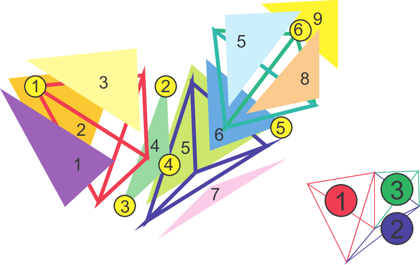
Figure 9.1: A simple 3-complex used for a running example of the implementation of the Extended Winged  data structure.

TV[1..3,0..3]
	0	1	2	3
1	1	2	3	4
2	2	3	4	5
3	2	4	5	6

VT*[1..6] 1 1 2 1 3 1 4 1 5 2 6 3 TT[1..3,0..3] 0 1 2 3 1 2 $\bot$ $\bot$ $\bot$ 2 $\bot$ 3 $\bot$ 1 3 $\bot$ $\bot$ $\bot$ 2

Figure 9.2: An example of TV,TT and $\mbox{\rm VT}^{\star}$ relations for the 3-complex of Figure 9.1

Note that sets of integers ${\rm Vertex}$ and ${\rm TopSimplex}$ need to be a set of consecutive integers. We will develop algorithms in this section using the identifier ${\rm Vertex}$ for the range $[{\rm MinV},\ldots,{\rm MaxV}]$ and the identifier ${\rm TopSimplex}$ for the range $[{\rm MinT},\ldots,{\rm MaxT}]$. This will be done to stress the fact that our results are still correct even if we take, for the sets ${\rm Vertex}$ and ${\rm TopSimplex}$, two sets of non contiguous, integers. This will be useful in Section 9.5.2 when we will merge all the TT, TV, and $\mbox{\rm VT}^{\star}$ arrays, one for each connected component, into two larger arrays TT’ and TV’ for all connected components of the original non-manifold complex. For optimization reasons, that will be apparent in Appendix B, in this merge will be useful to spread the range of indexes for TT into a non contiguous set of indexes for TT’. A similar scattering will be considered for indexes of TV over the array TV’.

TV and VT* Construction

We assume that, at the end of the decomposition process, we are left with a TV map ${\sigma_{TV}}:{{\rm TopSimplex}}\rightarrow{2^{{\rm Vertex}}}$ for each connected component of $\nabla\cdot{\Omega}$. We recall that we assume an implementation for these map that supports the sequential access to all elements in the domain of $\sigma_{TV}$ in constant time. Therefore, with a linear scan of the map $\sigma_{TV}$, we can fill the arrays TV and VT* in $\Theta(NT)$.

Therefore the construction of TV and $\mbox{\rm VT}^{\star}$ relations do not pose particular problems. Some more details are needed to show how to fill the TT array.

Example 9.4.3.

In Figure 9.2 we report the result of filling TV and VT* arrays for the 3-complex in Figure 9.1.

TT Construction

The TT array, that encodes the TT relation, is is filled in two steps. First we build a map ${\sigma_{{\mathcal{A}}}}:{\Omega^{[h-1]}}\rightarrow{{\bf listof}\,\,{\rm TopSimplex}}$. Upon completion of this first step, the domain of the map ${\sigma_{{\mathcal{A}}}}$ will be the set of $(h-1)$-simplices in $\nabla\cdot{\Omega}$. For each $(h-1)$-simplex $\psi$ the map ${\sigma_{{\mathcal{A}}}}[\psi]$ will give the list of indexes for the top $h$-simplices that are cofaces of $\psi$.

In a second step we fill the TT array in a way such that TT[$t$,$k$] will be the top simplex adjacent to simplex $t$ and such that the vertex TV[$t$,$k$] is not in the top simplex TT[$t$,$k$]. Thus TT[$t$,$k$] points the top simplex adjacent to $t$ and incident to its $(h-1)$-face that do not contain vertex TV[$t$,$k$].

Such a top simplex do not exist whenever the $(h-1)$-face of $t$ that do not contain the vertex TV[$t$,$k$] is on the boundary. In this case we put $TT[$t,k$]=\bot$.

Example 9.4.4.

In Figure 9.2 we report what must contain the TT array for the 3-complex in Figure 9.1.

Whenever the complex is non-pseudomanifold we will find situations where two or more top simplices satisfy the above condition for $t$. In this situation we treat this condition in a way similar to a boundary condition and put $TT[$t,k$]={\Upsilon}$ This is the main difference between this structure and the classical Winged Representation. An alternative approach to this construction, that organize top simplices adjacent to a non-pseudomanifold $(h-1)$-simplex into a cycle using will be presented in Section 9.4.4.

To sketch the construction algorithm we need to use sets of vertex indexes and maps from sets of vertex indexes to sets of top simplices. To comply with requirements of section 9.3.4 we assume that sets of vertex indexes can be ordered in the following way. We will say that the set of vertices $s_{1}$ is smaller than $s_{2}$ iff the ordered sequence of vertices in $s_{1}$ is lexicographically smaller than the ordered sequence of vertices in $s_{2}$. Thus for instance set $s_{1}=\{3,2,1\}$ is smaller than $s_{2}=\{1,4,2\}$. In fact the ordered sequence of elements in $s_{1}$ is ${<\!1,2,3\!\!>}$ while the ordered sequence of elements in $s_{2}$ is ${<\!1,2,4\!\!>}$. Lexicographic comparison shows that ${<\!1,2,3\!\!>}$ is smaller than ${<\!1,2,4\!\!>}$.

Finally we assume to have a function OPPOSITE(TV,$t$,$\psi$) that returns the position in the array TV[$t$] of the vertex in the top $h$-simplex $t$ that is not in its $(h-1)$-face $\psi$ (i.e. the vertex in $t$ opposite to $\psi$). In other words the function OPPOSITE must satisfy the assertion: TV[$t$,OPPOSITE(TV,$t$,$\psi$)]$\not\in\psi$. With this assumptions we lay the algorithm to fill the TT array as follows:

Algorithm 9.4.1 (Fill the TT array).

 

  var $\sigma_{{\mathcal{A}}}$: map set of Vertex into list of TopSimplex;

  $\sigma_{{\mathcal{A}}}\leftarrow(\forall x)[x\mapsto{<\!\mbox{}\!\!>}]$ {initially the map $\sigma_{{\mathcal{A}}}$ always returns the empty list}

  for all $t\in{\rm TopSimplex}$ do

     $\gamma\leftarrow$ set(TV[$t$])

     for all $v\in\gamma$ do

        ${{\sigma_{{\mathcal{A}}}}[\gamma-\{v\}]}\leftarrow{<\!t\!\!>}+{{\sigma_{{\mathcal{A}}}}[\gamma-\{v\}]}$ {add $t$ to the previous value of ${\sigma_{{\mathcal{A}}}}[\gamma-\{v\}]$}

     end for

  end for

  for all $\psi$ in the domain on $\sigma_{{\mathcal{A}}}$ do

     $star_{\psi}\leftarrow\sigma_{{\mathcal{A}}}[\psi]$ {$star_{\psi}$ is the list of cofaces of $(h-1)$-simplex $\psi$}

     if $star_{\psi}={<\!t\!\!>}$ then {$\psi$ is on the boundary}

        TT[$t$,OPPOSITE(TV,$t$,$\psi$)]=$\bot$ {$\bot$ stands for no adjacency}

     else if $star_{\psi}={<\!t,t^{\prime}\!\!>}$ then {$\psi$ is a manifold $(h-1)$-simplex}

        TT[$t$,OPPOSITE(TV,$t$,$\psi$)]=$t^{\prime}$

        TT[$t^{\prime}$,OPPOSITE(TV,$t^{\prime}$,$\psi$)]=$t$

     else {$\psi$ is a non-manifold $(h-1)$-simplex}

        TT[$t$,OPPOSITE(TV,$t$,$\psi$)]=${\Upsilon}$ {${\Upsilon}$ stands for non-manifold adjacency}

     end if

  end for

 

Example 9.4.5.

As an example we report the Algorithm 9.4.1 commented with assertions that applies when filling TT array for the 3-complex in Figure 9.1. Loops and instructions within loops are commented with an assertion that holds only the first time the loop is executed. With this convention this example shows how are filled two entries, i.e. TT[1,0]=2 and TT[2,3]=1 in the table TT of Figure 9.2. The annotated algorithm also shows some actual values for this tiny complex.

  var $\sigma_{{\mathcal{A}}}$: map set of 1..6 into list of 1..3;

  $\sigma_{{\mathcal{A}}}\leftarrow(\forall x)[x\mapsto{<\!\mbox{}\!\!>}]$

  for all $t\in{\tt 1..3}$ do {$t=1$}

     $\gamma\leftarrow$ set(TV[$t$]) {$\gamma=\{1,2,3,4\}$}

     for all $v\in\gamma$ do {$v=1$}

        ${{\sigma_{{\mathcal{A}}}}[\gamma-\{v\}]}\leftarrow{<\!t\!\!>}+{{\sigma_{{\mathcal{A}}}}[\gamma-\{v\}]}$ {${{\sigma_{{\mathcal{A}}}}[\{2,3,4\}]={<\!1\!\!>}}$}

     end for

  end for

  for all $\psi$ in the domain on $\sigma_{{\mathcal{A}}}$ do {$\psi=\{2,3,4\}$}

     $star_{\psi}\leftarrow\sigma_{{\mathcal{A}}}[\psi]$ {$star_{\psi}={<\!1,2\!\!>}$}

     if $star_{\psi}={<\!t\!\!>}$ then {$\psi=\{2,3,4\}$ is not on the boundary, skip}

        TT[$t$,OPPOSITE(TV,$t$,$\psi$)]=$\bot$ {$\bot$ stands for no adjacency}

     else if $star_{\psi}={<\!t,t^{\prime}\!\!>}$ then {${<\!t,t^{\prime}\!\!>}={<\!1,2\!\!>}$}

        TT[$t$,OPPOSITE(TV,$t$,$\psi$)]=$t^{\prime}$ {TT[1,0]=2 since OPPOSITE(TV,1,$\{2,3,4\}$)=0}

        TT[$t^{\prime}$,OPPOSITE(TV,$t^{\prime}$,$\psi$)]=$t$ {TT[2,3]=1 since OPPOSITE(TV,2,$\{2,3,4\}$)=3}

     else {$\psi$ is a non-manifold $(h-1)$-simplex}

        TT[$t$,OPPOSITE(TV,$t$,$\psi$)]=${\Upsilon}$ {${\Upsilon}$ stands for non-manifold adjacency}

     end if

  end for

If we postulate a standard implementation for maps and sets, then the following fact holds:

Property 9.4.1.

Let the TV array the encoding of a TV relation for a regular $h$-complex $\Omega$ with $NT$ $h$-simplices. Then the Algorithm 9.4.1 computes the TT relation for $\Omega$ and completes in $O(h^{2}NT\log{NT})$

Proof 9.4.6.

To evaluate the time complexity of Algorithm 9.4.1 we assume that we can use a standard implementation for lists, sets and maps as postulated in Section 9.3. When we use maps that have sets as keys (as in ${\sigma_{{\mathcal{A}}}}[\gamma-\{v\}]$) we have to consider the fact that each key must be lexicographically compared. Since sets are kept ordered into BSTs the comparison between two sets of $h$ elements can be done in $O(h)$.

With our assumption about sets we have that all the array-to-set conversions performed by calls to set(TV[$t$]) are done in $O(h\log{h}\cdot NT)$. The construction of $\sigma_{{\mathcal{A}}}$ is done updating this map at most $(h+1)NT$ times. For each update we retrieve the list ${{\sigma_{{\mathcal{A}}}}[\gamma-\{v\}]}$ and add an element. Since the list can be updated in constant time the whole construction of $\sigma_{{\mathcal{A}}}$ can be done with $O(h\cdot NT\log{NT})$ comparisons between arguments of the form $(\gamma-\{v\})$. Each comparison is in $O(h)$. Therefore the overall time complexity for the construction of $\sigma_{{\mathcal{A}}}$ must be $O(h^{2}NT\log{NT})$. Upon termination of this phase the map ${\sigma_{{\mathcal{A}}}}[\psi]$ gives the $h$-simplices incident at the $(h-1)$-simplex $\psi$.

Next we fill the array TT that has, at most, $(h+1)NT$ entries. Actually we consider only $(h-1)$-simplices that have at most two incident $h$-simplices. To fill each entry we have to compute OPPOSITE(TV,$t$,$\psi$). This gives the correct TT entry to store into and proves the correctness of algorithm. The computation of OPPOSITE can be done testing for all elements in TV[$t$] if they are in the set $\psi$. This takes at most $h\log{h}$. Therefore we can fill TT in $O(h^{2}NT\log{h})$ and, assuming that $h<NT$, we can say that the whole construction can be done in $O(h^{2}NT\log{NT})$

TT Navigation and retrieval of $S_{{0h}}(v)$ in Initial-quasi-manifolds

The TT array encodes the TT relation, therefore for every top $h$-simplex indexed by $t$, we have that:

1. for $k=0\ldots h$ the top simplex recorded in TT[$t$,$k$] is adjacent with $t$;

2. the simplices indexed by $t$ and TT[$t$,$k$] shares a $(h-1)$-simplex that do not contains the vertex indexed by TV[$t$,$k$].

These two facts that comes directly from the definition of the TT relation, easlily implies the following property

Property 9.4.2.

Let $v$ be a vertex of simplex $t$ such that TV[$t$,$h$]$=v$ and let $t^{\prime}=$TT[$t$,$k$] for some $k\neq h$. Then the top simplices $t$ and $t^{\prime}$ are adjacent and they both belongs to the star of $v$.

Example 9.4.7.

As an example we consider the 3-complex in Figure 9.1 and the table TT of Figure 9.2. Let’s take $t=2$ and $v=5$. With this choice we have that TV[2,3]=5 so we take $h=3$ and $k=0,1,2$. Among TT[2,0], TT[2,1] and TT[2,2] only for $k=1$ TT[2,1] returns a tetrahedron that is tetrahedron 3 that actually shares a triangle with tetrahedron 2. Tetrahedra 2 and 3 belongs to the star of vertex 5. The vertex TV[2,1] is vertex 3 that is neither in the star of 5 nor in the triangle shared by tetrahedra 2 and 3.

Considering the above property and the fact that our complex is an initial-quasi-manifold we have that the set of top simplices in $\star{v}$ can be collected simply using the TT relation. In fact we can travel completely the star of a vertex by adjacency because, in an initial-quasi-manifold, the star of each vertex must be $(h-1)$-manifold-connected.

Therefore, we are ready to devise an algorithm for computation of $S_{{0h}}(v)$ in an $h$-complex:

In the following pseudocode we will use lists as defined in Section 9.3.2 and a bit vector of $\Theta$ of $NT$ bits, i,e., one bit for each top simplex in the complex (see Section 9.3.3 for the definiton of bit vectors).

$\Theta$ : array $[{\rm MinT},\ldots,{\rm MaxT}]$ of bit.

This bit vector will be used to mark top simplices visited by our algorithm. We assume that when the application is started this bit vector is allocated

With these ancillary data structures it easy to devise an algorithm for the computation of $S_{{0h}}(v)$ in a generic $h$-complex:

Algorithm 9.4.2 (Computation of $S_{{0h}}(v)$ in an initial-quasi-manifold $h$-complex).

 

  Function $S_{{0h}}(v:{\tt Vertex})$ returns list of TopSimplex

  $N\leftarrow S\leftarrow{\bf list}(\sigma_{VT^{\star}}(v))$

  while $N\neq{<\!\mbox{}\!\!>}$ do

     $t\leftarrow N.{\rm TOP}$; $N\leftarrow N.{\rm POP}$; $\Theta[t].{\rm SET}$

     for $k=0$ to $h$ do

        if TV[$t$,$k$]$\neq v$ then

           $t^{\prime}\leftarrow$ TT[$t$,$k$]

           if not $\Theta[t^{\prime}].{\rm TEST}$ and $t^{\prime}\neq\bot$ and $t^{\prime}\neq{\Upsilon}$ then

              $N\leftarrow{<\!t^{\prime}\!\!>}+N$; $S\leftarrow{<\!t^{\prime}\!\!>}+S$

           end if

        end if

     end for

  end while

  for all t in S do

     $\Theta[t].{\rm CLEAR}$

  end for

  return $S$

 
Following the informal idea given in the introduction to this algorithm we can prove the following property stating algorithm total correctness.

Property 9.4.3.

Let $\Omega$ be an initial-quasi-manifold $h$-complex. For any vertex $v\in\Omega$ the above algorithm for $S_{{0h}}(\{v\})$ terminates. Upon termination in the variable $S$ we find the list of elements in the set $S_{{0h}}(\{v\})$.

Proof 9.4.8.

By Property 9.4.2 we have that all simplices added to $S$ belongs to the star of $v$. To prove termination we note that this computation cannot loop indefinitely because of the following facts:

• a simplex is added to the list $N$ iff it is added to $S$;

• a simplex already in $S$ is not added to $N$;

• the algorithm cannot loop for more than $h+1$ steps without deleting an element in $N$.

So to loop indefinitely the algorithm must add continuously elements in $N$ and therefore an indefinite number of new elements must come into $S$. This is impossible because $S$ is a subset of the star of $v$.

Obviously the computation for $S_{{0h}}(v)$ returns a subset of the star of $v$. We note that during the computation of $S_{{0h}}$ if a simplex $t$ is inserted in $S$ then all the simplices that are manifold adjacent w.r.t. $t$ will be inserted in $S$, if not already in. By transitivity all simplices in the star of $v$ that are $(h-1)$-manifold-connected with those in $S$ will eventually fit into $S$. Being within an initial-quasi-manifold $h$-complex the star of $v$ is $(h-1)$-manifold-connected by Property 7.4.3 Part 3. Therefore upon termination $S$ must contain the star of $v$.

The above algorithm computes $S_{{0h}}(v)$ in optimal time i.e. in $\Theta(|S_{{0h}}(v)|)$. This is stated in the following property.

Property 9.4.4.

The computation of $S_{{0h}}(v)$ takes $\Theta(h|S_{{0h}}(v)|)$.

For each top simplex inserted in $N$ we perform $(h+1)$ access to the TV table and next performs $h$ times the test $\Theta[t^{\prime}].{\rm TEST}$. Assuming a standard implementation for the bit vector we can perform this test in constant time for an overall complexity of $\Theta(h)$ comparisons for each top simplex added to $N$. All other operations take a constant time and are performed once for each element in the output All simplices inserted in $N$ are recorded in $S$ and therefore the total number of elements added to $N$ is given by the size of the output of the set $S_{{0h}}={S_{{0h}}(v)}$. Therefore the algorithm perform a loop for each element added in the output. Thus we have a total complexity of $\Theta(h|S_{{0h}}|)$.

Initial-quasi-manifold Navigation and the computation of $S_{{nm}}(\gamma)$

In the previous section we presented an algorithm for the computation of ${S_{{0h}}}$ In this section we present a couple of algorithms needed for the computation of and of ${S_{{nm}}}$ for $n<m$. Next we evaluate the time complexity of these algorithms. First we need to develop a function FaceOf($m,\beta$,CoTop) that returns the list of $m$-cofaces of $\beta$ that are $m$-faces of $h$-simplices in CoTop. The algorithm is developed assuming that all $h$-simplices in CoTop are cofaces of $\beta$. In other words the function FaceOf is defined by the equation:

$${\rm FaceOf}(m,\beta,CoTop)=\{\gamma|\mbox{\rm dim}(\gamma)=m\,\mbox{\bf and}\,(\exists\tau\in CoTop)(\beta\leq\gamma\leq\tau)\}$$

This auxiliary function can be computed in $O(|CoTop|)$ using the following algorithm:

Algorithm 9.4.3 (Computation of FaceOf($m,\beta$,CoTop)).

 

  FaceOf($m$, $\beta$: set of Vertex, CoTop: list of (set of Vertex)) returns list of (set of Vertex) var Inserted[$10\cdot{h+1\choose m+1}|CoTop|$]: hashed set of (set of Vertex).

  Result$\leftarrow{<\!\mbox{}\!\!>}$

  $n\leftarrow|\beta|$

  for all $\tau\in CoTop$  do

     $\psi\leftarrow\tau-\beta$

     for all $\{v_{0},\ldots,v_{m-n}\}\subset\psi$ do

        Face $\leftarrow\beta\cup\{v_{0},\ldots,v_{m-n}\}$

        if Face $\not\in$ Inserted then {Face not already in}

           Result $\leftarrow{<\!{\rm Face}\!\!>}$ + Result;

           Inserted $\leftarrow$ Inserted $\cup\{{\rm Face}\}$;

        end if

     end for

  end for

 
The correctness of the above algorithm is obvious. Its complexitiy is discussed by the following property:

Property 9.4.5.

The algorithm 9.4.3 is linear in the size of the input CoTop

Proof 9.4.9.

All operations needed to generate Face can be done in $O(h\log{h})$, being $h$ the dimension of the complex. We have taken in the implementation the variable ”Inserted” as an hash set. The size of this hash table is taken ten times ${h+1\choose m+1}|CoTop|$. The number ${h+1\choose m+1}|CoTop|$ represents an upper bound for the number of $m$-faces of simplices in CoTop. Due to this space provision for variable ”Inserted”, marking and testing in the hash set ”Inserted” can be considered to be done in constant time.

The test Face $\not\in$ Inserted is performed at most ${h+1\choose m+1}|CoTop|$. Thus the overall execution time must be in $O({h\log{h}}{{h+1\choose m+1}|CoTop|})$.

Using the auxiliary function FaceOf, the $S_{{nm}}(\gamma)$ relation can be computed following the algorithm below:

Algorithm 9.4.4 (Computation of $S_{{nm}}(\gamma)$ in a initial-quasi-manifold $h$-complex).

 

  Function $S_{{nm}}(\gamma:\mbox{\bf set of }{\tt Vertex})$ returns list of (set of Vertex)

  select $v$ in $\gamma$

  $S_{{0h}}\leftarrow S_{{0h}}(v)$; $Top\leftarrow{<\!\mbox{}\!\!>}$

  for all $t\in S_{{0h}}$ do

     $\theta\leftarrow$ set(TV[$t$]);

     if $\gamma\subset\theta$ then

        $Top\leftarrow{<\!\theta\!\!>}+Top$

     end if

  end for

  return FaceOf($m$,$\gamma$,$Top$)

 
We assume that the statement select $v$ in $S$ randomly select an element in $S$. It is easy to see that the algorithm above computes the total function $S_{{nm}}(\gamma)$ for every $\gamma\in\Omega$. The time complexity of this computation in general is not optimal as it shows the following property.

Property 9.4.6.

The computation of $S_{{nm}}(\gamma)$ can be done in $O(h|S_{{0h}}(v)|)$.

Proof 9.4.10.

The computation of $S_{{nm}}(\gamma)$ accounts for an initial computation of $S_{{0h}}(v)$ for some $v\in\gamma$. This, by property 9.4.4, takes $\Theta(h|S_{{0h}}(v)|)$. We will show that this dominates the complexity of all other operations. Having computed $S_{{0h}}(v)$ we are left with a set of $|S_{{0h}}(v)|$ top $h$-simplices with $h>n+m$. For each one of these top simplices we check if $\gamma$ is a subset of $\theta$. This inclusion check can be done in $\Theta(n\log{(h)})$ for a total complexity of $\Theta(n\log{(h)}|S_{{0h}}(v)|)$. From the subset of top simplices left we generate all $m$-faces that include $\gamma$. This is done with the call to FaceOf($m$,$\gamma$,$Top$) that takes $O(|Top|)$ Since elements in $Top$ are a subset of the elements in $|S_{{0h}}(v)|$ thus this operation must be in $O(h|S_{{0h}}(v)|)$. This completes the proof.

We notice that the expressions for the complexity of $S_{{nm}}(v)$ are only partially satisfactory since they do not give an expression that relates complexity of the computation with the size of the output Indeed the retrieval of topologic relations within this data structure can require the exploration of all top simplices around a vertex. thus the complexity for ${S_{{nm}}(\gamma)}$ depends on $\Theta(S_{{0h}}(v))$ for some $v\in\gamma$.

Obviously for $n>0$ the extraction of ${S_{{nm}}(\gamma)}$ can be grossly inefficient (See Property 9.2.6 in the next section) but this is a direct consequence of the fact that $n$-simplices do not receive a explicit representation in this data structure. In section 9.5.5 we will show that we can enrich this data structure with an indexing structure and obtain optimal extraction of ${S_{{nm}}(\gamma)}$ for $n>0$.

However, in this section we raise the question whether this data structure is acceptable at least for the extraction of topological relations among the entities that are explicitly modeled (i.e. vertices). More precisely we want to show when the data structure can extract in optimal time $S_{{0m}}$ for $0<m<h$. In the next subsection we will show that for certain class of complexes the idea of running around a vertex $v$ to find all top simplices do not impair the optimality of the extraction process, even if we are just interested in $m$-simplices.

9.4.3 Performance for $S_{0m}$

The algorithm for the computation of $S_{nm}$ is only partially satisfactory because its complexity, in general, do not depends on the size of the output. On the other hand, as we have shown, our data structure, in general, supports the optimal computation of ${S_{0h}(v)}$ in an $h$-complex. In fact ${S_{0h}(v)}$ can be recovered in $O(h|{S_{0h}(v)}|)$. Since in this data structure vertices receive explicit representation we expect that also all the $S_{0m}$ relations, for $0<m<h$ can be extracted in optimal time.

In this section, we will show that optimal extraction of $S_{0m}$, for $0<m<h$, is possible for initial-quasi-manifold surfaces and for initial-quasi-manifold tetrahedralizations that are embeddable in ${\rm I\kern-1.99997ptR}^{3}$ as a compact geometric simplicial complex. In particular we will show that in manifold surfaces $S_{01}(v)$ is computable in $O(|{S_{01}(v)}|)$. Similarly we will show that in a initial-quasi-manifold $3$-complex embeddable in ${\rm I\kern-1.99997ptR}^{3}$ $S_{01}(v)$ is computable in $O(|{S_{01}(v)}|)$ and $S_{02}(v)$ is computable in $O(|{S_{02}(v)}|)$. To this aim we will use the relation between face numbers we introduced in Section 9.2.2.

Manifold Surfaces

We know that all initial-quasi-manifold surfaces are manifold surfaces and, in turn, manifold surfaces are pseudomanifolds. Thus we can apply linear inequalties for face numbers we have introduced in Section 9.2.2. In particular we will use the fact that $\frac{3}{2}f_{2}\leq f_{1}$.

We have that $S_{01}(v)$ is computable in $O(|{S_{02}(v)}|)$. Being ${|S_{02}(v)|}=f_{2}(\star{v})$ and being $\frac{3}{2}f_{2}\leq f_{1}$ (see Equation 9.4 and apply some algebra) we have that $S_{01}(v)$ is computable in $O(|{S_{01}(v)}|)$. This proves that, at least for initial-quasi-manifold surfaces, the extraction algorithm is optimal for the computation of $S_{01}(v)$, too.

Simplicial $h$-complexes imbeddable in ${\rm I\kern-1.99997ptR}^{h}$

Next we will show that our data structure supports optimal extraction of topological relations also for tetrahedralizations that can be embedded in ${\rm I\kern-1.99997ptR}^{3}$. To this aim, in this section, we will use the linear inequalities between face numbers $f_{h}$, $f_{h-1}$ and $f_{h-2}$ we have developed in Section 9.2.2. From this we will derive that, for a complex imbeddable in ${\rm I\kern-1.99997ptR}^{h}$, the number of elements in $S_{0h}(v)$ is $O(|S_{0m}(v)|)$ for all $(h-3)\leq m\leq(h-1)$. From this it is easy to prove that the proposed algorithm is optimal for the extraction of $S_{0m}$ for $(h-2)\leq m\leq h$ whenever the given $h$-complex is embeddable in ${\rm I\kern-1.99997ptR}^{h}$. This will prove that our extraction algorithm is optimal for the computation of $S_{01}$ and $S_{02}$ for initial-quasi-manifold tetrahedralizations embeddable in ${\rm I\kern-1.99997ptR}^{3}$. In particular this proves that our algorithm is optimal for the extraction of all vertex based topological relations for initial-quasi-manifold tetrahedralizations embeddable in ${\rm I\kern-1.99997ptR}^{3}$. This is expressed by the following property.

Property 9.4.7 (Optimality for $S_{0(h-1)}$ $S_{0(h-2)}$).

The computation of $S_{0m}$ for $(h-2)\leq m\leq h$ for an initial-quasi-manifold $h$-complex $\Omega$ can be done in $O(|S_{0m}|)$ whenever the given abstract simplicial complex is embeddable in ${\rm I\kern-1.99997ptR}^{h}$.

Proof 9.4.11.

We already know that computation of $S_{0m}$ for an initial-quasi-manifold $h$-complex can be done in $O(|S_{0h}|)$. Thus properties 9.2.1 and 9.2.2 shows that $|S_{0h}|$ is both $O(|S_{0(h-1)}|)$ (by Property 9.2.1) and $O(|S_{0(h-2)}|)$ (by Property 9.2.2). This proves that the computation of $S_{0m}$ can be done in $O(|S_{0m}|)$ for all $(h-2)\leq m\leq h$.

Non-optimal Extraction in $4$-manifolds

Although we have assessed the optimality of vertex based extractions for tetrahedralizations in ${\rm I\kern-1.99997ptR}^{3}$. A natural question is what happens for $4$-complexes. By property 9.4.7 we know that if the $4$-complex is an initial-quasi-manifold embeddable in ${\rm I\kern-1.99997ptR}^{4}$ our data structure supports optimal extraction of relations $S_{04}$, $S_{03}$ and $S_{02}$, while the optimal extraction of $S_{01}$ is not assured. In this section we will prove that our algorithm is not always optimal for the extraction of $S_{01}$ in a $4$-complexes. Next we will show that non optimal extraction exist in $3$-complexes not embeddable in ${\rm I\kern-1.99997ptR}^{3}$. To this aim we will use the results of Section 9.2.2

For the $4$-dimensional case it is possible to build a triangulation of the $4$-ball where there is at least a vertex $w$ for which the extraction of $S_{01}(w)$ takes much more than $|S_{01}(w)|$. To build such a complex we just have to take as $4$-simplex the triangulation of the $4$-ball mentioned in Property 9.2.4 obtained as the cone from an arbitrary vertex $w$ to the boundary of the Cyclic Polytope in ${\rm I\kern-1.99997ptR}^{4}$.

Property 9.4.8.

There exist a triangulation $TB^{4}$ of the $4$-ball imbeddable in ${\rm I\kern-1.99997ptR}^{4}$ and a vertex $w$ such that the extraction of $S_{01}(w)$ following algorithm 9.4.4 takes $\Omega(|S_{01}(w)|^{2})$.

Proof 9.4.12.

As $4$-complex we take the triangulation $TB^{4}$ of the $4$-ball mentioned in Property 9.2.4. This ensure that there is a vertex $w$ for which $f_{4}(\overline{star({w},{TB^{4}})})=f_{0}(f_{0}-3)/2$ with $f_{0}$ the number of vertices in $\overline{star({w},{TB^{4}})}$. Next we consider the computation of $S_{01}(w)$ and recall that the computation of $S_{01}(w)$ implies the computation of $S_{04}(w)$. Thus we have that the computation of $S_{01}(w)$ is $\Omega({|S_{04}(w)|})$. For the $4$-complex $TB^{4}$ we have that ${|S_{04}(w)|}=f_{3}({\partial C_{4}(f_{0})})=f_{0}(f_{0}-3)/2$ where $f_{0}$ must be ${|S_{01}(w)|}$. Thus, for this particular $4$-complex, the computation of $S_{01}(w)$ takes $\Omega(|S_{01}(w)|^{2})$. Thus our algorithm fails to be optimal for a $4$-complexes embeddable in ${\rm I\kern-1.99997ptR}^{4}$.

The above Property generalize to $h$-balls showing that the extraction of $S_{01}(w)$ is non-optimal and can become quite inefficient as $h$ grows.

Property 9.4.9.

There exist a triangulation $TB^{h}$ of the $h$-ball embeddable in ${\rm I\kern-1.99997ptR}^{h}$ such that, for a certain vertex $w$ in $TB^{h}$, the extraction of $S_{01}(w)$, performed by algorithm 9.4.4 is non-optimal and is $\Omega(|S_{01}(w)|^{\left\lfloor{h/2}\right\rfloor})$.

Proof 9.4.13.

By Property 9.4.9 we know that there exist a triangulation $TB^{h}$ of the $h$-ball embeddable in ${\rm I\kern-1.99997ptR}^{h}$ such that, for a certain vertex $w$ in $TB^{h}$, $f_{h}(\overline{star({w},{TB^{h}})})=\Theta(f_{0}^{\left\lfloor{h/2}\right\rfloor})$ with $f_{0}$ is the number of vertices in $\overline{star({w},{TB^{h}})}$. Next we consider the computation of $S_{01}(w)$ and recall that the computation of $S_{01}(w)$ implies the computation of $S_{0h}(w)$. Thus we have that the computation of $S_{01}(w)$ is $\Omega({|S_{0h}(w)|})$. For the complex $TB^{h}$ we have that ${|S_{0h}(w)|}=f_{h}(\overline{star({w},{TB^{h}})})=\Theta(f_{0}^{\left\lfloor{h/2}\right\rfloor})$ with $f_{0}$ is the number of vertices in $\overline{star({w},{TB^{h}})}$. Therefore $|S_{01}(w)|$ is $\Omega(|S_{01}(w)|^{\left\lfloor{h/2}\right\rfloor})$.

Following Property 9.2.6 it is easy to build an $h$-ball $TB^{h}$, for $h$ sufficiently high, in which there exist an $n$-simplex $\gamma$ for which $S_{n(n+1)}(\gamma)$ is $\Omega(|S_{n(n+1)}(\gamma)|^{2})$. The property below, as formal statement of this fact, gives a concrete reference for our claim for non optimality of $S_{nm}$ we gave in Section 9.4.2.

Property 9.4.10.

For any natural $n>0$, there exist a combinatorial $h$-ball $TB^{h}$ that can be embedded in ${\rm I\kern-1.99997ptR}^{h}$, for $h=4+n$, and an $n$-simplex $\gamma$ such that the computation of $S_{n(n+1)}(\gamma)$ is $\Theta(|S_{n(n+1)}(\gamma)|^{2})$.

Proof 9.4.14.

By Property 9.2.6, for $h=4+n$, there exist a combinatorial $h$-ball $TB^{h}$ that can be embedded in ${\rm I\kern-1.99997ptR}^{h}$, $f_{h}(\overline{star({\gamma},{TB^{h}})})=f_{0}(f_{0}-3)/2$ with $f_{0}$ the number of vertices in $\overline{star({\gamma},{TB^{h}})}$ that are not in $\gamma$.

By Property 9.4.4 we have that the computation of $S_{n(n+1)}(\gamma)$ can be done in $\Theta(|S_{0h}(v)|)$ being $v$ a vertex in $\gamma$. By the way we have built $TB^{h}$ $|S_{0h}(v)|=f_{h}(\overline{star({\gamma},{TB^{h}})})=f_{0}(f_{0}-3)/2$ and therefore, with some easy algebra, we show that the computation of $S_{n(n+1)}(\gamma)$ is $\Theta(f_{0}^{2})$ .i.e. $\Theta(|S_{n(n+1)}(\gamma)|^{2})$.

Thus, also the computation of $S_{nm}(\gamma)$ in an $h$-complex might become grossly inefficient for $m=n+1$. Finally, combining the proof above and that of Property 9.2.5 it is easy to build an $h$-complex $B^{h}$, for $h$ sufficiently high, in which there exist a $n$-simplex $\gamma$ for which $S_{n(n+1)}(\gamma)$ is $\Theta(|S_{n(n+1)}(\gamma)|^{\left\lfloor{h/2}\right\rfloor})$.

Non-optimal Extraction in non embeddable $3$-manifolds

The above property shows that the algorithm 9.4.4 is non optimal in dimension higher than three. Lack of optimality is also present in relation extraction for $3$-complexes if we drop the requirement on embeddability in ${\rm I\kern-1.99997ptR}^{3}$. This is an easy consequence of properties developed in Section 9.2.2.

Property 9.4.11.

There exist countably many initial-quasi-manifold $3$-complexes $B(g)$, for any natural $g>0$, not embeddable in ${\rm I\kern-1.99997ptR}^{3}$, such that there exist a vertex $w$ for which $|S_{03}(w)|=\Theta(|S_{01}(w)|^{2})$. In particular we have ${{(S_{01}^{2}-3S_{01}+8)}/3}<S_{03}\leq{{S_{01}(S_{01}-1)}/3}$.

Proof 9.4.15.

The proof builds easily upon the result in Property 9.2.7 Taking the family of $3$-complexes $B(g)$ mentioned in this property and the associated vertex $w$ and reasoning as in the proof of Property 9.2.4 we show that in $B(g)$ we have $|S_{03}(w)|=\Theta({|S_{01}(w)|}^{2})$.

9.4.4 Extended Winged Data Structure for non-pseudomanifolds

In this section we describe a further extension for the extended winged data structure (EWDS) that will be crucial in Section 9.5.2 to travel the star of a generic $n$-simplex $\gamma$ in an initial-quasi-manifold. In fact, in an initial-quasi-manifold $h$-complex, the star of a vertex must be $(h-1)$-manifold connected. This condition ensures the correctness of the extraction algorithms 9.4.2 and 9.4.4. Whenever we pretend to travel the star of an arbitrary $n$-simplex, for $n>0$, we cannot assume this star to be manifold-connected. Thus, in this section, we will present a revised version of the extended winged representation that takes into account non-pseudomanifold adjacencies. This will allow to navigate the star of $\gamma$ whenever this is $(h-1)$-connected even if it is not $(h-1)$-manifold connected. Next in section 9.5.4 we will introduce the $\sigma_{\nabla}$ relation that will allow to jump from one $(h-1)$-connected component into another $(h-1)$-connected component in the star of a given simplex $\gamma$. These two extension will allow to retrieve in optimal time all top simplices in the star of a arbitrary simplex. This extension to the EWDS exploits the fact that some features in this data structure were left unspecified or unused. In particular we will use the indexes of the TT relation holding the symbol ${\Upsilon}$ to express non-pseudomanifold adjacencies.

We recall that an initial-quasi-manifold $d$-complex in general is not a $d$-pseudomanifold. In Example 7.4.2 we have shown that this is the case for $d\geq 3$. However we can ensure that the star of each vertex, in an initial-quasi-manifold $h$-complex, is manifold-connected and this supports the correctness of the algorithms developed so far. Thus a first thing to note is that using the ${\Upsilon}$ simbol for other purposes do not impair neither the correctness nor the complexity of the given algorithms that remain the same.

The idea at the basis of this extension is that we can use indexes previously set to ${\Upsilon}$ to connect the three or more $h$-simplexes sharing the same $(h-1)$-simplex, in a non-pseudomanifold initial-quasi-manifold. This extension do not require to modify the algorithm for the extraction of $S_{0m}$. We simply have to modify the way in which the TT relation is built. Therefore we adopt the assumption of Section 9.3.2 about lists. In particular we recall that is possible to have a method to retrieve, in constant time, one after one, all elements in a list. When list $l$ is used to control an iteration we recall that $l.CircularNext$ can be used to fetch, in the list $l$, the element after the one currently returned for the iteration, w.r.t. the circular order induced by the list $l$.

With these assumptions it easy to see that the following algorthm do the job and fills the TT array without using the symbol ${\Upsilon}$. In the following we will assume that this algorithm is used instead of Algorithm 9.4.1 to fill the TT array in the EWDS we use.

Algorithm 9.4.5 (Fill the TT array for non-pseudomanifolds).

 

  var $\sigma_{{\mathcal{A}}}$: map set of Vertex into list of TopSimplex;

  $\sigma_{{\mathcal{A}}}\leftarrow(\forall t)[t\mapsto{<\!\mbox{}\!\!>}]$ {initially the map $\sigma_{{\mathcal{A}}}$ always returns the empty list}

  for all $t\in{\rm TopSimplex}$ do

     $\gamma\leftarrow$ set(TV[$t$])

     for all $v\in\gamma$ do

        ${{\sigma_{{\mathcal{A}}}}[\gamma-\{v\}]}\leftarrow{<\!t\!\!>}+{{\sigma_{{\mathcal{A}}}}[\gamma-\{v\}]}$ {add simplex $t$ to the list in ${\sigma_{{\mathcal{A}}}}[\gamma-\{v\}]$}

     end for

  end for

  for all $\psi$ in the domain on $\sigma_{{\mathcal{A}}}$ do

     $l\leftarrow\sigma_{{\mathcal{A}}}[\psi]$

     if $l={<\!t\!\!>}$ then

        TT[$t$,OPPOSITE(TV,$t$,$\psi$)]=$\bot$ {$\bot$ stands for no adjacency}

     else

        for all  $t$ in $l$  do

           TT[$t$,OPPOSITE(TV,$t$,$\psi$)]=$l$.CircularNext

        end for

     end if

  end for

 
This algorithm has the same requirements and performance of the Algorithm 9.4.1 from which it is derived. In fact all added operations can be done in constant time and each added operation sets an entry that the previous algorithm was filling with ${\Upsilon}$. A ${\Upsilon}$ entry is used, in the previous algorithm, when there are three or more top simplices $t_{1},t_{2},\ldots,t_{n}$ that are jointly adjacent. In the new TT relation, now we have a sequence of $n>2$ indexes $j_{1},j_{2},\ldots,j_{n}$ such that, whenever in the previous algorithm we had TT[$t_{k}$,$j_{k}$]=${\Upsilon}$ now we have: $t_{k+1}=TT[t_{k},j_{k}]$ for $1\geq k\geq n$ with $t_{n+1}$=$t_{1}$.

Remark 9.4.16.

This extension require a slight modification in the definition of the generalized winged representation that is the main component of the extended winged representation. We recall that, in definition 9.4.1, we required that the relation ${\mathcal{A}}\subset\Theta^{2}$ must be a subset of the TT relation for $\Omega$ such that $\theta_{1}{\mathcal{A}}\theta_{2}$ iff the simplex shared by top simplexes (indexed by) $\theta_{1}$ and $\theta_{2}$ is a manifold simplex in $\Omega$. Now we extend this definition by removing this requirement and simply ask that the relation ${\mathcal{A}}\subset\Theta^{2}$ must be a subset of the TT relation for $\Omega$. In the following we will assume that the extended winged representation satisfy this, more general, definition.

9.5 The Non-manifold Layer

In the previous section we have considered the problem of representing a single initial-quasi-manifold component through the Extended Winged Representation. This representation is the basis for the lower layer of our two layer data structure. In this section we introduce the Non-manifold Winged representation and give a rationale for this representation. Next we define a data structure to store this representation and evaluate its space requirements. We will give procedures to build this data structures using the output of the decomposition process. Finally we will show that the two layers together supports the extraction of all topological relations in $O(n\log{n})$ for a $h$-complex for $h\leq 3$, being $n$ the size of the output.

In general, for $h>3$ for an $h$-complex embeddable in ${\rm I\kern-1.99997ptR}^{h}$, the two layer data structure supports the extraction of $S_{0m}$ for $(h-2)\leq m\leq h$ and the extraction of $S_{nm}$ for $(h-3)\leq n<m\leq h$ in $O(n\log{n})$ . On the other hand, as already shown in Property 9.4.9, for instance, for $4$-complexes the extraction of relation $S_{01}$ is non-optimal.

9.5.1 The Non-manifold Winged Representation

To give the definition of the Non-manifold Winged we need some preliminary notation. If $\Omega$ is an abstract simplicial complex with Vertices in $V$ and top simplices in $\Theta$ we will use the notation $\nabla\cdot{V}$ and $\nabla\cdot{\Theta}$ to denote, respectively, the set of vertices and top simplices in $\nabla\cdot{\Omega}$. We will denote with $\mathcal{N}M$ the subset of non-manifold $n$-simplices $\gamma$ in $\Omega$ having one these two problem:

• the simplex $\gamma$ is a splitting simplex w.r.t. the decomposition $\nabla\cdot{\Omega}$;

• the simplex $\gamma$ is not splitting simplex and its star in $\nabla\cdot{\Omega}$ is not $(h-1)$-connected.

Note that the second issue can occur only for an $n$-simplex $\gamma$ for $n>0$. Indeed for $n=0$ we know that the star of a vertex in an $h$-component in $\nabla\cdot{\Omega}$ is always $(h-1)$-connected being $\nabla\cdot{\Omega}$ an initial-quasi-manifold (see Definition 7.4.6 and Property 8.3.4). We will denote with $\nabla\cdot{\mathcal{N}M}$ the set of all simplex copies for all simplices in $\mathcal{N}M$. Note that non-splitting simplices in $\mathcal{N}M$ remains in $\nabla\cdot{\mathcal{N}M}$, too. In Figure 9.3 there is an example of an initial-quasi-manifold  3-complex. In this non-manifold complex the star of the orange central edge is made up of the two colored tetrahedra. Thus the orange edge has a star that is not a 2-connected complex. Therefore, the set $\mathcal{N}M$ for this complex is the singleton containing the orange edge.

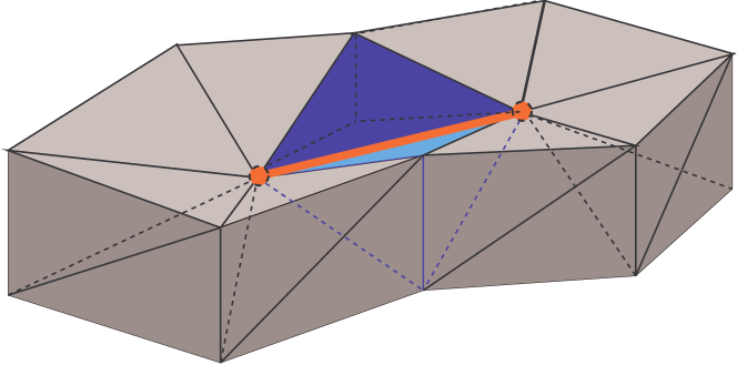
Figure 9.3: A 3-complex in which the central orange edge has a star that is not 2-connected.

Note that in general, in the following, we will use primed symbols (e.g. $\gamma^{\prime}$) for elements in $\nabla\cdot{\Omega}$ and non primed symbols for the corresponding element in $\Omega$. Whenever the operator $\nabla$ is used in our notation we will define things so that the element coming from the not decomposed complex must stay after $\nabla$, as in $\nabla\cdot{\Omega}$, while the elements from $\Omega$ are usually placed before $\nabla$. With this idea in mind we can introduce the pair of relations $\nabla$ and ${\geq^{\nabla}}^{\star}$ that represents the upper layer of our two layer representation.

The first relation combines a splitting simplex $\gamma\in\Omega$ with all its simplex copies $\gamma^{\prime}\in\nabla\cdot{\Omega}$. We will write ${\gamma^{\prime}}\nabla{\gamma}$ to mean that $\gamma^{\prime}$ is a simplex copy for $\gamma$.

The second relation ${\geq^{\nabla}}^{\star}$ is a subset of the restriction of the face relation to the set ${(\nabla\cdot{\Theta})\times(\nabla\cdot{\mathcal{N}M})}$. This simply means that whenever ${\theta^{\prime}}{\geq^{\nabla}}^{\star}{\gamma^{\prime}}$ we must have that ${\gamma^{\prime}}\in\nabla\cdot{\mathcal{N}M}$ and ${\theta^{\prime}}\in\nabla\cdot{\Theta}$ and $\theta^{\prime}\geq\gamma^{\prime}$. This sub relation is not uniquely identified but it must satisfy the following requirements:

• first we ask ${\theta^{\prime}}{\geq^{\nabla}}^{\star}{\gamma^{\prime}}$ for some top simplex $\theta^{\prime}\in\nabla\cdot{\Theta}$ if and only if  $\overline{star({\gamma^{\prime}},{\nabla\cdot{\Omega}})}$ has at least two $(h-1)$-connected components;

• second, we ask that for each $(h-1)$-connected component in the $\overline{star({\gamma^{\prime}},{\nabla\cdot{\Omega}})}$ there must be one and only one top simplex $\theta^{\prime}\in\nabla\cdot{\Omega}$ such that ${\theta^{\prime}}{\geq^{\nabla}}^{\star}{\gamma^{\prime}}$;

With the above notations we can define the Non-manifold Winged  Representation as follows:

Definition 9.5.1.

If $\Omega$ is an abstract simplicial complex with Vertices in $V$ and top simplices in $\Theta$ then the Non-manifold Winged Representation for $\Omega$ is a triple $NMWS=(EWS,\nabla,{\geq^{\nabla}}^{\star})$ where:

• $EWS$ is an Extended Winged Representation for $\nabla\cdot{\Omega}$;

• the relation $\nabla\subset(\nabla\cdot{\Omega})\times\Omega$ is such that${\gamma^{\prime}}\nabla{\gamma}$ if and only if  $\gamma$ is a splitting simplex and $\gamma^{\prime}$ is one of its simplex copies;

• the relation ${\geq^{\nabla}}^{\star}\subset(\nabla\cdot{\Theta})\times(\nabla\cdot{\mathcal{N}M})$ is such that the following conditions are satisfied:

  1. for each $(h-1)$-connected component in the star $star({\gamma^{\prime}},{\nabla\cdot{\Omega}})$ there exist a top simplex $\theta^{\prime}\in\nabla\cdot{\Omega}$ for which ${\theta^{\prime}}{\geq^{\nabla}}^{\star}{\gamma^{\prime}}$;

  2. if ${\theta_{1}^{\prime}}{\geq^{\nabla}}^{\star}{\gamma^{\prime}}$ and ${\theta_{2}^{\prime}}{\geq^{\nabla}}^{\star}{\gamma^{\prime}}$ then $\theta_{1}$ and $\theta_{2}$ must belong to two distinct $(h-1)$-connected component in the star $star({\gamma^{\prime}},{\nabla\cdot{\Omega}})$

We will refer to the couple of relations $\nabla$ and ${\geq^{\nabla}}^{\star}$ as the upper layer of our two layer representation. On the other hand the $EWS$ Extended Winged Representation will be referred as the lower layer of the Non-manifold Winged Representation

To define a data structure for this representation we assume that is possible to represent the complex $\nabla\cdot{\Omega}$ with a global Extended Winged Data Structure obtained by the merge of all data structures for each connected component in $\nabla\cdot{\Omega}$. We assume that exists a data type named EWDS for such a data structures. In particular if $NV^{\prime}$ and $NT^{\prime}$ are respectively the number of vertices and top simplices in $\nabla\cdot{\Omega}$. Obviously $NT=NT^{\prime}$ but we choose to use two different symbols to have a uniform notation. We assume that the declaration ${\bf var}EWS:EWDS(NV^{\prime},NT^{\prime})$ expands to the declaration of a valid data structure to encode $\nabla\cdot{\Omega}$. The data structure for EWDS is developed from data structure in 9.4.1. The EWDS data structure and its optimization will be discussed in the following Section 9.5.2.

With these assumptions the data structure encoding the Non-manifold Winged is the following:

Data Structure 9.5.1 (Non-manifold Winged Data Structure for $\Omega$).

 

type
	Vertex = [1..NV];$\{$range of indexes for vertices of $\Omega$ $\}$
	TopSimplex = [1..NT];$\{$range of indexes for top simplices of $\Omega$ $\}$
	Simplex = set of Vertex;$\{$a generic simplex of $\Omega$ represented as a set of vertex indexes $\}$
	Vertex’ = [1..NV’];$\{$range of indexes for vertices of $\nabla\cdot{\Omega}$ $\}$
	TopSimplex’ = [1..NT’];$\{$range of indexes for top simplices of $\nabla\cdot{\Omega}$ $\}$
	Simplex’ = set of Vertex’;$\{$a generic simplex of $\nabla\cdot{\Omega}$ represented as a set of vertex indexes $\}$
var
	EWS	: EWDS(NV’,NT’);
		$\{$ A Global Extended Winged Data Structure for $\nabla\cdot{\Omega}$ (see Section 9.5.2)$\}$
	$\sigma$	: map of Vertex’ into Vertex; $\sigma^{-1}$	: map of Vertex into set of Vertex’;$\{$See Section 9.5.3$\}$
		$\{$$\sigma[v^{\prime}]$ maps a vertex copy $v^{\prime}$ into the corresponding splitting vertex in ${\Omega}$ $\}$
		$\{$$\sigma^{-1}[v]$ maps a splitting vertex $v$ into the set of its corresponding vertex copies in $\nabla\cdot{\Omega}$ $\}$
	$\sigma_{\nabla}$	: map of Simplex into (map of Simplex’ into set of TopSimplex’);
		$\{\theta\in\sigma_{\nabla}[\gamma][\gamma^{\prime}]$ if and only if  ($\gamma=\gamma^{\prime}\mbox{ \bf or }{\gamma^{\prime}}\nabla{\gamma})\mbox{ \bf and }{\theta^{\prime}}{\geq^{\nabla}}^{\star}{\gamma^{\prime}}\}$ (see Section 9.5.4)

 
As reported before, note that in this data structure definition, we have used primed identifiers (e.g. Vertex’) to denote elements that refers to the decomposition $\nabla\cdot{\Omega}$. Similarly will use primed letters, e.g. $v^{\prime}$, $\gamma^{\prime}$ to denote elements in the decomposition $\nabla\cdot{\Omega}$. Plain letters and identifiers (e.g. Vertex) are used for elements that refers to $\Omega$.

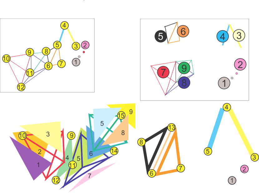
Figure 9.4: A 3-complex $\Omega$ used for a running example of the implementation of the Non-manifold Winged Representation. On the top left we have the un-decomposed complex $\Omega$. Note that we do not stitch to the definition On the top right the decomposed complex $\nabla\cdot{\Omega}$ with top simplices numbering. In larger bottom figure vertices numbers are given in yellow balls. Note that, due to the addition of dimensionally mixed parts, the vertices and simplices numbers are different from those in Figure 9.1. All other numbers are for $(h-1)$ simplices in the $h$-complexes in the decomposition.

Example 9.5.2.

With reference to Figure 9.4 we can begin a chain of running examples where we apply the concepts so far defined. Up to now we can say that for this complex the first part of the data structure rewrites as

type
	TopSimplex = [1..9];$\{$range of indexes for vertices of $\Omega$ $\}$
	Vertex = [1..12];$\{$range of indexes for vertices of $\Omega$ $\}$
	Vertex’ = [1..15];$\{$range of indexes for vertices of $\nabla\cdot{\Omega}$ $\}$
	TopSimplex’ = [1..9];$\{$range of indexes for top simplices of $\nabla\cdot{\Omega}$ $\}$

being NV=12, NT=9,NV’=15 and NT=NT’=9.

9.5.2 A Global Data Structure for $\nabla\cdot{\Omega}$

We can build, quite easily, a single Extended Winged data structure EWDS(NV’,NT’) that contains the representation for all the initial-quasi-manifold components of $\nabla\cdot{\Omega}$. Let $\Omega$ be a $d$-complex with Vertices in $V$ and top simplices in $\Theta$ (note that $d$ is used for the dimension of the complex ${\Omega}$ and $h$ for the dimension of each component in $\nabla\cdot{\Omega}$). A global data structure for $\nabla\cdot{\Omega}$ is the following:

Data Structure 9.5.2 (Global Extended Winged Data Structure for $\nabla\cdot{\Omega}$).

 

type
	Vertex’ = [1..NV’];
	TopSimplex’ = [1..NT’];
	INDEX =[1..SIZE];
var
	TV’:array[][][] of Vertex’;
	TT’:array[][][] of TopSimplex’;
	VT*’:array[1..NV’] of TopSimplex’;
	TBase,TBaseAddr:array[0..D] of INDEX;

 
Where $NT^{\prime}$ and $NV^{\prime}$ are, respectively the number of top simplices and of vertices in the decomposition $\nabla\cdot{\Omega}$. To build a global data structure for $\nabla\cdot{\Omega}$ we simply have to take the data structures for each components in $\nabla\cdot{\Omega}$ (see the Data Structure 9.4.1) and assume that the ranges of indexes ${\rm Vertex}=[{\rm MinV},\ldots,{\rm MaxV}]$ and ${\rm TopSimplex}=[{\rm MinT},\ldots,{\rm MaxT}]$ for different components are a partition of the the larger ranges, $[1,\ldots,NV^{\prime}]$ and $[1,\ldots,NT^{\prime}]$.

We can assume that space for the TT, TV and TV* arrays for each decomposition components is allocated in non overlapping sub-areas within the areas for the corresponding TT’, TV’and TV*’ arrays. We assume that allocation starts from components of dimension $0$ and goes up. That is to say elements in lower dimensional components receive lower indexes.

Note that within the TT’ and TV’ arrays coexist slices of different length. This require some ancillary data structures for indexing. To this goal ve provided the ${\rm TBase}$ and the ${\rm TBaseAddr}$ arrays. We discuss in the next lines details of this allocation mechanism. With the notation TV’:array[][][] of Vertex’; and TT’:array[][][] of TopSimplex’; we denote arrays whose three ranges are not known at compile time. These array will be allocated dynamically to the size given by ${\rm SIZE}=\sum_{0\leq h\leq d}{|\Theta^{[h]}|(h+1)}$, where with $\Theta^{[h]}$ we denote the set of top $h$-simplices. In the following discussion we assume that we can use each of these two arrays as large unidimensional arrays ${\rm TT^{\prime}}[1,\ldots,{\rm SIZE}]$ and ${\rm TV^{\prime}}[1,\ldots,{\rm SIZE}]$.

The occupation of the Global Extended Winged Data Structure is given by the following property:

Property 9.5.1.

Let $\Omega$ a $d$-complex with top simplices in $\Theta$ and vertices in $V$. Let $NS$ and $NC$ be respectively the number of splitting vertices and the number all vertices that are the vertex copies of the $NS$ splitting vertices standard decomposition $\nabla\cdot{\Omega}$. In this situation the TT’, TV’, VT*’ arrays in the Global Extended Winged Data Structure takes

$${\rm SIZE}\cdot(\log{NT^{\prime}}+\log{NV^{\prime}})+NV^{\prime}\log{NT^{\prime}}\,\mbox{\rm bits}$$

where: ${\rm SIZE}=\sum_{0\leq h\leq d}{|\Theta^{[h]}|(h+1)}$, with $\Theta^{[h]}$ the set of top $h$-simplices in $\Omega$. $NT^{\prime}=\sum_{0\leq h\leq d}{|\Theta^{[h]}|}$ is the number of top simplices in $\Omega$ and $NV^{\prime}=|V|-NS+NC$.

Proof 9.5.3.

It is easy to see that the number $NV^{\prime}$ of vertices in $\nabla\cdot{\Omega}$ is given by $NV^{\prime}=|V|-NS+NC$. On the other hand the number of top simplices is NT’ both in $\Omega$ and in $\nabla\cdot{\Omega}$. The TT’, TV’, VT*’ arrays in the global data structure takes ${\rm SIZE}\cdot(\log{NT^{\prime}}+\log{NV^{\prime}})+NV^{\prime}\log{NT^{\prime}}$ bits to store $\nabla\cdot{\Omega}$. This formula comes easily from thee fact that $\log{NV^{\prime}}$ bits are used to code a pointer to a vertex for each top simplex in the TV’ array. Thus an $h$ top simplex takes $(h+1)\log{NV^{\prime}}$ bits and all $h$ top simplices take $|\Theta^{[h]}|(h+1)\log{NV^{\prime}}$. Summing for all $h$ we obtain ${\rm SIZE}\cdot(\log{NV^{\prime}})$ bits occupation for TV’. Then $\log{NT^{\prime}}$ bits are necessary to code a reference to a top simplex in the TT’ table, so summing all over the TT’ table we obtain an occupation of ${\rm SIZE}\cdot(\log{NT^{\prime}})$ bits. Then Finally the VT*’ table has NV’ entries each storing a pointer to a top simplex taking $\log{NT^{\prime}}$ bits for an overall sum of $NV^{\prime}\log{NT^{\prime}}$. This completes the proof.

An obvious possible space optimization can be implemented by coding these $\log{NT^{\prime}}$ and $\log{NV^{\prime}}$ pointers as displacements within the ranges of ${\rm Vertex}=[{\rm MinV},\ldots,{\rm MaxV}]$ and ${\rm TopSimplex}=[{\rm MinT},\ldots,{\rm MaxT}]$.

In the array element ${\rm TBase}[h]$ we store the index assigned to the first top $h$-simplex. In the array element ${\rm TBaseAddr}[h]$ we store the base address to access data for $h$-simplices in TT’ and TV’ arrays. More precisely ${\rm TBaseAddr}[h]$ stores the index of the last element of the last slice of $h$ elements within the TT’ and TV’ arrays. The array ${\rm TBase}$ is filled when we build the global data structure for $\nabla\cdot{\Omega}$ by counting the number of top $h$-simplices inserted. We will put ${\rm TBase}[h]={\rm TBase}[h+1]$ if no top $h$-simplex exist. When the array ${\rm TBase}[h]$ is filled the array ${\rm TBaseAddr}[h]$ is computed using the recurrence ${\rm TBaseAddr}[0]=1$ and

$${\rm TBaseAddr}[h+1]={\rm TBaseAddr}[h]+(h+1)({\rm TBase}[h+1]-{\rm TBase}[h])$$

For a top $h$-simplex that received as index $t^{\prime}$ we will retrieve the TT slice of length $h+1$ starting beyond TT’[TBaseAddr[$h$]+$(t^{\prime}-{\rm TBase}[h])(h+1)$]. Similarly we will retrieve the TV slice of length $h+1$ starting beyond TV’[TBaseAddr[$h$]+$(t^{\prime}-{\rm TBase}[h])(h+1)$]. In the following we will forget these access details and use the shortcuts:

$${\rm TT^{\prime}}[h,t^{\prime},k]=\\ {{\rm TT^{\prime}}[{\rm TBaseAddr}[h]+(t^{\prime}-{\rm TBase}[h])(h+1)+k-1]}\mbox{ with }1\leq k\leq h+1$$ (9.8)

$${\rm TV^{\prime}}[h,t^{\prime},k]=\\ {{\rm TV^{\prime}}[{\rm TBaseAddr}[h]+(t^{\prime}-{\rm TBase}[h])(h+1)+k-1]}\mbox{ with }1\leq k\leq h+1$$ (9.9)

Note that this is just a convenient notation and must be implemented directly (for instance using macros in C). In fact such an array, where the range of the second and third index depends upon the value of the first index are not supported by standard programming languages.

We note that the dimension of a top simplex $t^{\prime}$ can be computed in $\Theta(d)$ by finding the index $h$ for which ${\rm TBase}[h]\leq t^{\prime}<{\rm TBase}[h+1]$. Thus in the following we will use the notation $\mbox{\rm dim}(t^{\prime},\nabla\cdot{\Omega})$ to denote the result of this computation, i.e. the dimension of the simplex (indexd by) $t^{\prime}$. In general we will denote with $\mbox{\rm dim}(v^{\prime},\nabla\cdot{\Omega})$ the dimension of the component of $\nabla\cdot{\Omega}$ to which $v^{\prime}$ belongs to. The function $\mbox{\rm dim}(v^{\prime},\nabla\cdot{\Omega})$ can be computed in $\Theta(d)$ with using the $\mbox{\rm VT}^{\star}$ relation with the formula $\mbox{\rm dim}(v^{\prime},\nabla\cdot{\Omega})=\mbox{\rm dim}(\sigma_{VT^{\star}}(v^{\prime}),\nabla\cdot{\Omega})$. Similarly for a simplex $\gamma^{\prime}\in\nabla\cdot{\Omega}$ we will define $\mbox{\rm dim}(\gamma^{\prime},\nabla\cdot{\Omega})$ as $\mbox{\rm dim}(\gamma^{\prime},\nabla\cdot{\Omega})=\mbox{\rm dim}(v^{\prime},\nabla\cdot{\Omega})$ for some $v^{\prime}\in\gamma^{\prime}$. When this is not ambiguous we will use simply $\mbox{\rm dim}(\gamma^{\prime})$ as a shortcut for $\mbox{\rm dim}(\gamma^{\prime},\nabla\cdot{\Omega})$

Example 9.5.4.

We continue our running example started at Example 9.5.2. W.r.t. Figure 9.4 we can say that, in the situation of Property 9.5.1 we have $d=3$, NS=3 and NC=6. The top simplices are of order 0,1,2,3 and we have $\Theta^{[0]}=2$, $\Theta^{[1]}=2$, $\Theta^{[2]}=2$ and $\Theta^{[3]}=3$. Therefore SIZE must be 24. The arrays TBaseand TBaseAddr are filled as shown in Figure 9.5. To play with them we can try to develop the expression in Formula 9.9

$${\rm TV^{\prime}}[2,5,3] = {{\rm TV^{\prime}}[{\rm TBaseAddr}[2]+(5-{\rm TBase}[2])(2+1)+3-1]}$$

$$= {\rm TV^{\prime}}[7+(5-5)3+3-1]={\rm TV^{\prime}}[9]=8$$

i.e. the third vertex of 2-simplex 5 is 8. Next we report in Figure 9.6 the complete filling of TV’ and TT’.

TBase[0..3]
0	1
1	3
2	5
3	7

TBaseAddr[0..3] 0 1 1 3 2 7 3 13

Simplex	@	TV’[1..24]				Comment
1	1	1				TBaseAddr[0]=1
2	2	2
3	3:4	3	4			TBaseAddr[1]=3
4	5:6	4	5
5	7:9	6	13	8		TBaseAddr[2]=7
6	10:12	6	7	13
7	13:16	10	9	12	11	TBaseAddr[3]=13
8	17:20	9	12	11	14
9	21:24	9	11	14	15	SIZE=24

Figure 9.5: An example of arrays TBase, TBaseAddr, TV’for the 3-complex of Figure 9.4. Note that in these tables the values in contiguous cells in the array TV’, whenever needed, are grouped horizontally in slices. Thus $x:y$ on the @ column corresponds to $y-x+1$ cells on the right, showing values stored at $x,x+1,\ldots,y$. Vector VT*’ is represented horizontally simply to save space.

VT*’[1..15]
1	2	3	4	5	6	7	8	9	10	11	12	13	14	15
1	2	3	3	4	6	6	5	7	7	7	7	5	8	9

Simplex	@	TT’[1..24]				Comment
1	1	$\bot$				TBaseAddr[0]=1
2	2	$\bot$
3	3:4	4	$\bot$			TBaseAddr[1]=3
4	5:6	$\bot$	3
5	7:9	$\bot$	$\bot$	6		TBaseAddr[2]=7
6	10:12	$\bot$	5	$\bot$
7	13:16	8	$\bot$	$\bot$	$\bot$	TBaseAddr[3]=13
8	17:20	$\bot$	9	$\bot$	8
9	21:24	$\bot$	$\bot$	$\bot$	8	SIZE=24

Figure 9.6: An example of arrays TT’and VT*’ for the 3-complex of Figure 9.4. Vector VT*’ is represented horizontally simply to save space.

Example 9.5.5.

We continue our running example from Example 9.5.4. W.r.t. Figure 9.4 the arrays VT*’ and TT’ are filled as shown in Figure 9.6. To play with them we can try to develop the expression in Formula 9.8

$${\rm TT^{\prime}}[2,5,3] = {{\rm TT^{\prime}}[{\rm TBaseAddr}[2]+(5-{\rm TBase}[2])(2+1)+3-1]}$$

$$= {\rm TT^{\prime}}[7+(5-5)3+2]={\rm TT^{\prime}}[9]=6$$

i.e. the top 2-simplex adjacent to top 2-simplex 5 opposite to TV’[2,5,3] is 6. Indeed, from Example 9.5.5 we have TV’[2,5,3]=8 and looking at Figure 9.4 we can see that the triangle adjacent to 5 opposite to 8 is 6.

In the next section, we will discuss a possible space optimization that brings the size of our global data structure below the usual reference limit, attained by the Winged edge, of six pointers per triangle.

9.5.3 Splitting Vertices: Maps $\sigma$ and $\sigma^{-1}$ as a $\nabla$ restriction

In this section we start to discuss the relation $\nabla$ in the Non-manifold Winged Representation (see Definition 9.5.1). In particular we will introduce maps $\sigma$ and $\sigma^{-1}$. These two maps are mentioned in the Non-manifold Winged Data Structure 9.5.1. We will detail them here and define them as the restriction of relation ${\gamma^{\prime}}\nabla{\gamma}$ to pair of vertices. We first introduce some ideas and then state them formally giving a proof in Property 9.5.2.

To this aim we recall that, upon termination of the decomposition process, we are left with a simplicial complex $\nabla\cdot{\Omega}$ that represents the decomposition (see Algorithm 8.5.1). The decomposition Algorithm 8.5.1 can be patched to return some ancillary data structures. We will introduce here the patches and discuss the (negligible) impact on time complexity.

Indeed, upon completion of the decomposition process, we need to have a map ${\sigma}:{{\nabla\cdot{V}}}\rightarrow{V}$ that gives, for each vertex copy $v^{\prime}$ in $\nabla\cdot{\Omega}$ the corresponding splitting vertex in $\Omega$. We also assume that the decomposition process gives a set of Vertices $V_{\mathcal{N}M}$ with potential problems. The set $V_{\mathcal{N}M}$ and its construction will be described more precisely in Section 9.5.4.

We model the splitting process by the $\nabla$ relation in the upper layer of our representation. The relation $\nabla$ is a non symmetric relation $\nabla\subset(\nabla\cdot{V})\times V$. When restricted to Vertices the relation $\nabla$ relates each splitting vertex $v$ in $\Omega$, with the set of its vertex copies in $\nabla\cdot{\Omega}$. In other words ${v^{\prime}}\nabla{v}$ iff $v$ is a splitting vertex and $v^{\prime}$ is one of its vertex copies. More in general $\nabla$ is a relation between pairs of simplices, i.e. $\nabla\subset(\nabla\cdot{\Omega})\times\Omega$. We will write ${\gamma^{\prime}}\nabla{\gamma}$ whenever $\gamma^{\prime}$ is a splitting simplex for $\gamma$.

In the Non-manifold Winged Data Structure 9.5.1 we represent separately the restriction of $\nabla$ to set of vertices, i.e. the restriction of $\nabla$ to $(\nabla\cdot{V})\times V$. This portion of the relation $\nabla$ is represented with the two maps $\sigma^{-1}$ and ${\sigma}$. The map $\sigma$ can be constructed with a minor modification of the Algorithm 8.5.1 and the other map ${\sigma^{-1}}:{\nabla\cdot{V}}\rightarrow{V}$ is defined by the condition $v^{\prime}\in\sigma^{-1}[\sigma[v^{\prime}]]$.

We will extend $\sigma^{-1}$ and $\sigma$ to all Vertices in $\Omega$ and $\nabla\cdot{\Omega}$ by assuming $\sigma^{-1}(v)=\{v\}$ whenever $v$ is not a splitting vertex. Similarly we will pose $\sigma(v^{\prime})=v^{\prime}$ whenever $v^{\prime}$ is not a vertex copy. Given a simplex copy $\gamma^{\prime}$ in the decomposed complex we will denote with $\sigma(\gamma^{\prime})$ its translation into the original complex (i.e. $\cup_{v^{\prime}\in\gamma^{\prime}}{\sigma({v^{\prime}})}$). Similarly given a set of simplices $\Gamma\subset\nabla\cdot{\Omega}$ we define $\sigma(\Gamma)=\{\sigma(\gamma)|\gamma\in\Gamma\}$. These extensions are used for convenience in proofs and statements but it is not necessary to implement them, now. Actually only $\sigma$ and $\sigma^{-1}$ are detailed here.

The requirements for construction and storage of $\sigma$ and $\sigma^{-1}$ are given by the following property.

Property 9.5.2.

Let $NS$ be the number of splitting Vertices in $\Omega$ and let $NC$ be the total number of vertex copies introduced by the decomposition process. In this situation the following facts holds:

1. the construction of the map $\sigma$ takes $\Theta(NC\log{NC})$;

2. the construction of the map $\sigma^{-1}$ takes $\Theta(NC\log{NC})$;

3. the map $\sigma^{-1}$ takes up to $NS\log{NS}+NC\log{NC}$ bits to be encoded.

4. the map $\sigma$ takes up $NC(\log{NC}+\log{NS})$ bits to be encoded.

Proof 9.5.6.

We note, as detailed in 9.3.5, that a standard implementation for maps can attain a logarithmic access time.

Looking at Algorithm 8.5.1 it is easy to see that step 10 can be modified to build the $\sigma$ map with time complexity $\Theta(NC\log{NC})$. Indeed each vertex copy deserve just one attempt to be stored in $\sigma$. This storage is done in logarithmic time. Hence the map $\sigma$ can be constructed in $\Theta(NC\log{NC})$. This proves part 1. The original Algorithm 8.5.1 time complexity was $O({d!}\cdot(NT\log{NT}))$. Where $NT$ is the number of top simplices in the $d$-complex $\Omega$ (see 8.5.2). Being $NC\leq(d+1)\cdot NT$, we can say that this patch to line 10 of Algorithm 8.5.1 do not change its time complexity.

For proving the other parts we note that a standard implementations of maps usually supports sequential access to the elements of the domain of the map in constant time. Each entry in $\sigma^{-1}$ is a set of vertex copies and again we assume a standard implementation for these sets with a logarithmic access time. Thus, scanning the domain of the map $\sigma$, it is easy to build the map $\sigma^{-1}$ in $\Theta(NC\log{NC})$. This is done by the following fragment of code.

  for all $v^{\prime}\in{\rm domain}(\sigma)$ do

     ${\sigma^{-1}[\sigma[v^{\prime}]]}\leftarrow{\sigma^{-1}[\sigma[v^{\prime}]]}\cup\{v^{\prime}\}$

  end for

This is done in $O(NC\log{NC})$. In fact, it is easy to see, that this loop is executed once for each vertex copy $v^{\prime}$ and thus the loop gets executed $NC$ times. At each iteration we retrieve, modify and store back the entry ${\sigma^{-1}[\sigma[v^{\prime}]]}$. Modification is done in constant time and store and retrieval takes $O(\log{NS}+\log{NC})$, that is $O(\log{NC})$.

To analyze space requirements for these map we note that maps can be implemented with binary search trees (BST) that in turn can be implemented using heaps i.e. maintaining the BST a complete binary tree. Thus it can be represented with an array with just one index for each node in the tree. Thus, if $NS$ be the number of splitting Vertices in $\Omega$ then the map $\sigma^{-1}$ will take $NS\log{NS}$ bits for the indexing structure for this map. Similarly sets in map entries can be implemented as complete BST. Then we have that all sets takes less than $NC\log{NC}$ bits for all the sets of vertex copies. With these assumptions we have that $\sigma^{-1}$ takes up to $NS\log{NS}+NC\log{NC}$ bits to be encoded. No sets are needed for $\sigma$, being $\sigma(v^{\prime})$ a single vertex in $V$. Thus, the space requirement for the map $\sigma$ will be $NC(\log{NC}+\log{NS})$.

Finally we note that our data structure the Non-manifold Winged representation (see Definition 9.5.1) implicitly requires that vertex index used for a vertex $v$ in $\Omega$ is used again in $\nabla\cdot{\Omega}$ even if $v$ is a splitting vertex. So we assume that, when generating an index for a new vertex copy $v^{\prime}$, when splitting $v$, we store in $\sigma$ the same index for $v$ for the first copy and a brand new index only at the second try. With this last assumption we can draw a small example for the $\sigma$ and $\sigma^{-1}$ maps.

Example 9.5.7.

We continue our running example from Example 9.5.5. W.r.t. Figure 9.4 we have that the two maps $\sigma$ and $\sigma^{-1}$ must be.

$v$	$\sigma^{-1}$
5	$\{5,13\}$
6	$\{6,14\}$
8	$\{8,15\}$

$v^{\prime}$ $\sigma$ 5 $5$ 6 $6$ 8 $8$ 13 $5$ 14 $6$ 15 $8$

This completes the description and analysis of the two maps $\sigma$ and $\sigma^{-1}$ that are the first two elements in the upper layer of our representation. Using the data structures $\sigma$ and $\sigma^{-1}$ we can devise algorithms to extract, in optimal time, the topological relations $S_{0m}(\nabla\cdot{\Omega},v^{\prime})$, for $0<m\leq h$.

Extraction of $S_{0m}$ in the Non-manifold Complex

The two maps $\sigma$ and $\sigma^{-1}$ are sufficient to perform vertex based queries and navigation of a non-manifold complex $\Omega$ using the Extended Winged Representation of the decomposition $\nabla\cdot{\Omega}$. In fact starting from a vertex $v$ in $\Omega$ we can find all the topological relations $S_{0m}(\Omega,v)$ in $\Omega$ using the topological relations ${S_{0m}}$ in $\nabla\cdot{\Omega}$ following formula:

$${S_{0m}(\Omega,v)}=\bigcup_{v^{\prime}\in\sigma^{-1}[v]}{\sigma(S_{0m}(\nabla\cdot{\Omega},v^{\prime}))}$$ (9.10)

We must turn this formula into an algorithm with some care. The problem that requires some care is related to non regularity in the $\Omega$ complex. Indeed we must not perform the computation of $S_{0m}(\nabla\cdot{\Omega},v^{\prime})$ for those vertex copies $v^{\prime}$ that fall in an initial-quasi-manifold  of dimension strictly smaller than $m$.

With this caveat it is easy to translate formula 9.10 into an algorithm and it is easy to see that the computation of $S_{0m}(\Omega,v)$ can be done in optimal time only if $S_{0m}(\nabla\cdot{\Omega},v^{\prime})$ can be done in optimal time. However this condition might not be sufficient. We will see that this is a sufficient condition for $3$-complexes. In general, the algorithm for the computation of ${S_{0m}(\Omega,v)}$ is the following:

Algorithm 9.5.1 (Computation of $S_{0m}(\Omega,v)$).

 

  Function $S_{0m}(v:{\tt Vertex})$ returns set of Vertex

  if $v\in{\rm domain}(\sigma)$ then {$v$ is a splitting vertex}

     $VertexCopies\leftarrow\sigma^{-1}[v]$;

  else

     $VertexCopies\leftarrow\{v\}$;

  end if

  $Result\leftarrow\emptyset$;

  for all $v^{\prime}\in VertexCopies$ and $\mbox{\rm dim}{(v^{\prime},\nabla\cdot{\Omega})}\geq m$ do

     $Result\leftarrow Result\cup\sigma(S_{0m}(\nabla\cdot{\Omega},v^{\prime}))$ {refer to Algorithm 9.4.4 for $S_{0m}(\nabla\cdot{\Omega},v^{\prime})$}

  end for

  return $Result$;

 
According to the forthcoming results of Property 9.5.8 we have the following property.

Property 9.5.3.

Let $\Omega$ be a $d$-dimensional abstract simplicial complex  and let $v$ be a vertex in $\Omega$. In this situation the relation $S_{0m}({\Omega},v)$ in $\Theta(n\log{n})$, being $n$ the size of the output in the following cases:

• for $d=2$ and $1\leq m\leq 2$;

• for $d=3$ and $1\leq m\leq 3$ whenever $\Omega$ is embeddable in ${\rm I\kern-1.99997ptR}^{3}$;

Proof 9.5.8.

This property is a particular case of Property 9.5.8. The latter can be proven independently of this one, thus we reference to the proof of Property 9.5.8 for a proof of this property. Note that Property 9.5.8 deals about the computation of ${S_{0m}({\Omega},v|\theta^{\prime})}$ i.e. the computation of ${S_{0m}({\Omega},v)}$ provided that a top simplex $\theta^{\prime}$ incident to $v$ in $\Omega$ is known. This applies to this case since we can write ${S_{0m}({\Omega},v)}$ as ${S_{0m}({\Omega},v)}=S_{0m}({\Omega},v|VT*^{\prime}[v])$.

Optimal extraction is possible for $S_{01}$ and $S_{02}$ in $2$-complexes and for $S_{01}$, $S_{02}$ and $S_{03}$ in $3$-complexes embeddable in ${\rm I\kern-1.99997ptR}^{3}$ as compact geometric complexes. The extraction algorithm fail to be optimal for $4$-complexes For an example of non optimality of $S_{01}$ in a $4$-complex see Property 9.4.9.

9.5.4 Computation of $S_{nm}(\Omega,\gamma)$: the $\nabla$ and ${\geq^{\nabla}}^{\star}$ Relations and $\sigma_{\nabla}$

Introduction

In the previous section we have given a rationale for the introduction of $\sigma$ and $\sigma^{-1}$ by showing that these relations support the extraction of $S_{0m}$ in optimal time at least for $2$ and $3$-complexes. We note here that these two maps are necessary to develop such an extraction. The rationale for the introduction of $\nabla$, ${\geq^{\nabla}}^{\star}$ and $\sigma_{\nabla}$ is slightly different. We introduce the relations $\nabla$, ${\geq^{\nabla}}^{\star}$ in the Non-manifold Winged representation to support the computation of $S_{nm}(\Omega,\gamma)$ in optimal time. These relations are not necessary to perform this task. This is a consequence of the fact that the Extended Winged Representation match exactly the decomposition procedure and thus all information about the non-manifoldness that has been removed by the decomposition can be encoded in the $\sigma$ map. Furthermore this result is dimension independent.

In fact the computation of $S_{nm}(\Omega,\gamma)$ can be performed as follows. If $\gamma=\{v_{1},\ldots,v_{n}\}$ is an $n$-simplex in $\Omega$ it is easy to see that, for all $n\leq m$:

$$S_{nm}(\Omega,\{v_{1},\ldots,v_{n}\})=\bigcup_{v_{i}^{\prime}\in\sigma^{-1}(v_{i})}\sigma({S_{nm}(\nabla\cdot{\Omega},\{v^{\prime}_{1},\ldots,v^{\prime}_{n}\})})$$ (9.11)

It is easy to turn equation 9.11 into an algorithm. In fact the algorithm we have proposed for (the computation of) $S_{nm}(\nabla\cdot{(}\Omega),\gamma)$ (see Algorithm 9.4.4) gives a correct result (i.e. the empty set) even if the supplied argument $\{v^{\prime}_{1},\ldots,v^{\prime}_{n}\}$ is a set of $n$ Vertices that is not a simplex in $\nabla\cdot{\Omega}$.

Therefore the Extended Winged Data Structure extended with maps $\sigma$ and $\sigma^{-1}$ contains sufficient information to extract the topological relations $S_{nm}$. However this cannot be done in optimal time, In fact the extraction of $S_{nm}(\nabla\cdot{\Omega},\gamma)$, performed following Algorithm 9.4.4 can be grossly inefficient. In fact our algorithms always fetch a fan of top simplices around a vertex whatever will be the topological relation requested. In higher dimension and we have shown that, in some cases, for $m=n+1$, Algorithm 9.4.4 yields a processing time for $S_{n(n+1)}(\gamma)$ that is polynomial i.e. ${S_{n(n+1)}(\nabla\cdot{\Omega},\gamma)}$ is $\Theta(|S_{n(n+1)}(\nabla\cdot{\Omega},\gamma)|^{\left\lfloor{h/2}\right\rfloor}{\log{|S_{n(n+1)}(\nabla\cdot{\Omega},\gamma)|}})$. (see the remark at the end of Property 9.4.10).

In this section we will analyze and solve this problem introducing the $\nabla$ and ${\geq^{\nabla}}^{\star}$ relations.

The $S_{nh}(\Omega,\gamma|\theta)$ topological relation

A processing time of $\Theta(n^{\left\lfloor{h/2}\right\rfloor}{\log{n}})$ for the computation of ${S_{n(n+1)}(\nabla\cdot{\Omega},\gamma)}$ is not acceptable since the TT relation contains all information that are necessary to perform this computation in optimal time. We feel that this problem comes from two facts.

A first, quite obvious, fact is that both in the original Winged Representation and in the Extended Winged Representation in each $h$-dimensional component the $n$-simplices, for $0<n<h$, do not receive a direct representation. In fact we represent $n$-simplices as set of $n$ Vertices. For $n=0$ and $n=h$ we assign an explicit representation to $0$-simplices in the range $[1\ldots NV^{\prime}]$ and we assign an explicit representation to $h$-simplices in the range $[1\ldots NT^{\prime}]$. Representing explicitly $n$-simplices can be quite heavy and, furthermore, there are many situations in which this is not needed. In fact, there are situations in which we start from a top $h$-simplex $\theta$ and want to find all top $h$-simplices in the star $\star{\gamma}$ being $\gamma$ a proper face of $\theta$. In this case we will say that we want to compute the topologic relation $S_{nh}(\Omega,\gamma|\theta)$ (read $S_{nh}(\Omega,\gamma)$ given $\theta$). Next we take a retrieved $h$-simplex $\theta^{\prime}\in S_{nh}(\Omega,\gamma|\theta)$, select a face $\gamma^{\prime}\leq\theta^{\prime}$ and repeat this kind of query. In this case we do not need to introduce an explicit modeling entity for $n$-simplices. In fact, as we will show, our data structure can support the computation of $S_{nh}(\Omega,\gamma|\theta)$ in optimal time. So, in this section, we will discuss the $\nabla$ and ${\geq^{\nabla}}^{\star}$ relations that are introduced to support the computation of $S_{nh}(\Omega,\gamma|\theta)$ in optimal time. In Section 9.5.5 we will devise an auxiliary data structure, the $V^{n}T$ map, that introduces an explicit representation for $n$-simplices thus supporting the computation of $S_{nh}(\Omega,\gamma)$ in optimal time.

For sake of clarity we choose to leave the $V^{n}T$ out of the Non-manifold Winged Representation. In fact, the problem of giving an explicit representation to intermediate objects need not to be confused with the problem of representing non-manifoldness. Another benefit of the Non-manifold Winged is that these two aspects can be clearly identified and treated with separate mechanism.

To support the optimal computation of $S_{nh}(\Omega,\gamma|\theta)$ we need to take care of a second issue. In general, in an initial-quasi-manifold complex, the star $star({{\gamma}},{\Omega})$ of a generic $n$-simplex $\gamma$, for $n>0$, it is not $(h-1)$-connected. This might happen because $\gamma$ splits into several copies $\gamma^{\prime}_{i}$. However it is also possible to find complexes $\Omega$ for which $\Omega=\nabla\cdot{\Omega}$ and yet there exist an $n$-simplex $\gamma\in\Omega$ that have non-$(h-1)$-connected star. We have shown [36] that this problem do not depends on the particular decomposition process. In fact there are $h$-complexes, for $h\geq 3$, that can not be decomposed into a complex where all simplices has $(h-1)$-connected star. A complex where all the stars of all simplices are $(h-1)$-connected is called a regularly adjacent complex. A simplex whose star is $(h-1)$-connected will be called a regularly adjacent simplex. In Figure 9.3 we have shown an example of an initial-quasi-manifold 3-complex with a 2-simplex that is not regularly adjacent.

We note that the problem related to non-$(h-1)$-connectedness of a $n$-simplex stars is present if and only if  the complex $\Omega$ is a non-manifold complex. For this reason we do not want to solve this second problem adding a mechanism that adds extra memory when the complex $\Omega$ is regularly adjacent or even manifold. The introduction of the relations $\nabla$ and ${\geq^{\nabla}}^{\star}$ solves this problem in this direction and supports, with a small increase in memory requirements, the optimal computaton of $S_{nh}(\gamma|\theta)$

The $\nabla$ and ${\geq^{\nabla}}^{\star}$ Relations

Thus we want to overcome these two problems in order to obtain a data structure that supports the optimal extraction of $S_{nm}$ by adding an explicit representation just for the subset of non-manifold $n$-simplices $\gamma$ in $\Omega$ having one these two problem:

• the simplex $\gamma$ is a splitting simplex w.r.t. the decomposition $\nabla\cdot{\Omega}$;

• the simplex $\gamma$ is not splitting simplex and its star in $\nabla\cdot{\Omega}$ is not $(h-1)$-connected.

The set of simplices with one of these problems will be denoted by $\mathcal{N}M$. Similarly we will denote with $\nabla\cdot{\mathcal{N}M}$ the set of all simplex copies for all splitting simplices in $\mathcal{N}M$ plus all non-splitting simplices in $\mathcal{N}M$ (i.e. $\nabla\cdot{\mathcal{N}M}=\{\gamma^{\prime}|\sigma(\gamma^{\prime})\in\mathcal{N}M\}$). We first note that it might happen that the simplex $\gamma$ is a splitting simplex and still for one or more of its simplex copies $\gamma^{\prime}$ the complex $star({\gamma^{\prime}},{\nabla\cdot{\Omega}})$ is not $(h-1)$-connected. Second note that we simply ask for $(h-1)$-connectivity and not for $(h-1)$-manifold-connectivity. This is due to the possibilities offered by the optimization described in Section 9.4.4. In fact using the relation TT’, optimized deleting symbols ${\Upsilon}$, we can retrieve all the top simplices that are adjacent to a given simplex even if we traverse non-manifold $(h-1)$-simplices.

With the above discussion in mind, we are ready to devise completelty the two relations in the upper layer of our representation. We have already presented the relation $\nabla$ in Section 9.5.3 and we have encoded its restriction to $0$-simplices with the maps $\sigma$ and $\sigma^{-1}$. We choose to encode separately this restriction because, as shown by equation 9.11, these two maps are sufficient to extract all topological relations.

The second relation that is present in the Non-manifold Winged Representation, denoted by ${\geq^{\nabla}}^{\star}$, is the relation ${\geq^{\nabla}}^{\star}\subset\nabla\cdot{\Theta}\times\nabla\cdot{\mathcal{N}M}$ such that the following conditions are satisfied:

• for each $(h-1)$-connected component in the star $star({\gamma^{\prime}},{\nabla\cdot{\Omega}})$ there exist a top simplex $\theta^{\prime}\in\nabla\cdot{\Omega}$ for which ${\theta^{\prime}}{\geq^{\nabla}}^{\star}{\gamma^{\prime}}$;

• if ${\theta_{1}^{\prime}}{\geq^{\nabla}}^{\star}{\gamma^{\prime}}$ and ${\theta_{2}^{\prime}}{\geq^{\nabla}}^{\star}{\gamma^{\prime}}$ then $\theta_{1}$ and $\theta_{2}$ must belong to two distinct $(h-1)$-connected component in the star $star({\gamma^{\prime}},{\nabla\cdot{\Omega}})$

The $\sigma_{\nabla}$ Map

The remaining part of relation $\nabla$ and the ${\geq^{\nabla}}^{\star}$ relation will be jointly implemented in the Non-manifold Winged Data Structure by the map $\sigma_{\nabla}$. Putting together the two things, somehow, make things a little obscure. The remaining part of the relation $\nabla$ is the subset of the relation $\nabla\subset\nabla\cdot{\Omega}\times\Omega$ obtained deleting the couples in $\nabla\cdot{V}\times V$ from the relation $\nabla$. We will have that ${\gamma^{\prime}}\nabla{\gamma}$ if and only if  $\gamma$ is a splitting $n$-simplex and $\gamma^{\prime}$ is one of its simplex copies.

The two relations $\nabla$ and the ${\geq^{\nabla}}^{\star}$ are jointly coded into $\sigma_{\nabla}$ by taking map $\sigma_{\nabla}$ as a map that sends each simplex $\gamma\in\mathcal{N}M$ into a particular map. In other words the element returned by $\sigma_{\nabla}[\gamma]$ is a map ${\sigma_{\nabla}[\gamma]}:{(\nabla\cdot{\mathcal{N}M})}\rightarrow{2^{\nabla\cdot{\Theta}}}$. Sometimes, however, we will use $\sigma_{\nabla}[\gamma,\gamma^{\prime}]$ for $\sigma_{\nabla}[\gamma][\gamma^{\prime}]$. The most handy definition of $\sigma_{\nabla}$ is given by the procedure below

   Function $\sigma_{\nabla}(\gamma,\gamma^{\prime})$ returns subset of ${\nabla\cdot{\Theta}}$

  if $\gamma$ is a splitting simplex then {${\gamma^{\prime}}\nabla{\gamma}$}

     return$\{\theta_{1}\ldots\theta_{n}\}$ { Each $\theta_{i}$ from a distinct $(h-1)$-connected component in $star({\gamma^{\prime}},{\nabla\cdot{\Omega}})$}

  else

     if $\gamma$ is not a splitting simplex then {must be $\gamma=\gamma^{\prime}$}

        return$\{\theta_{1}\ldots\theta_{n}\}$ { Each $\theta_{i}$ from a distinct $(h-1)$-connected component in $star({\gamma^{\prime}},{\nabla\cdot{\Omega}})$}

     end if

  end if

Looking at $\sigma_{\nabla}$ as a map that returns a map we can say that the domain of the map $\sigma_{\nabla}[\gamma]$ (denoted by ${\rm domain}(\sigma_{\nabla}[\gamma])$ is the set of simplex copies for $\gamma$. This domain is a sigleton for all and alone simplices in $\mathcal{N}M$ that are not splitting simplices. Thus we have:

$${\gamma^{\prime}}\nabla{\gamma}\Leftrightarrow(\,{|{\rm domain}(\sigma_{\nabla}(\gamma))|>1}\,\mbox{\bf and }{\gamma^{\prime}\in{\rm domain}(\sigma_{\nabla}(\gamma))\,)}.$$ (9.12)

More in general, the map $\sigma_{\nabla}(\gamma)$ is defined completely by the condition:

$$\theta\in\sigma_{\nabla}[\gamma][\gamma^{\prime}]\Leftrightarrow((\,\gamma=\gamma^{\prime}\mbox{\bf or }{\gamma^{\prime}}\nabla{\gamma}\,)\mbox{\bf and }{\theta^{\prime}}{\geq^{\nabla}}^{\star}{\gamma^{\prime}}\,).$$ (9.13)

The implementation of this map can be done using a well known data structure for dictionaries called trie and is described in Section 9.5.5 together with the implementation of similar data structures that will be introduced later.

Example 9.5.9.

We continue our running example from Example 9.5.7. W.r.t. Figure 9.4 we have that $\sigma_{\nabla}[\gamma]$ is defined only for $\gamma=\{6,8\}$ and ${\rm domain}(\sigma_{\nabla}[\{6,8\}])=\{\{6,8\},\{14,15\}\}$

${\gamma^{\prime}}$	$\sigma_{\nabla}[\{6,8\}][{\gamma^{\prime}}]$
$\{6,8\}$	$\{5\}$
$\{14,15\}$	$\{9\}$

Construction of the map $\sigma_{\nabla}$

In this section we assume a standard implementation for this map and describe an algorithm to fill the $\sigma_{\nabla}$ map. Unless otherwise stated, in the description of this algorithm, we will use the greek primed letters, e.g. $\gamma^{\prime}$ and $\theta^{\prime}$, to denote simplices in $\nabla\cdot{\Omega}$ that are represented as sets of indexes. We will use latin letters, e.g. $t^{\prime}$ or $v^{\prime}$ to denote top simplices and vertices in $\nabla\cdot{\Omega}$ that are represented as sets of indexes.

This algorithm is described in two parts. First we develop a recursive procedure ${\rm TravelStar}(\gamma^{\prime},t^{\prime})$ that travels the star of $\gamma^{\prime}$ in $\nabla\cdot{\Omega}$ by adjacency, using the ${\mathcal{A}}$ relation (i.e. the TT’ array). The visit performed by ${\rm TravelStar}(\gamma^{\prime},t^{\prime})$ starts from top simplex $\theta^{\prime}$ and marks all visited top simplices. Marking of top simplices in $\nabla\cdot{\Omega}$ is performed setting a bit into an the array of bits

FT_FLAGS: array [1..NT’][1..2**(d+1)-2] of bits

All bits in this array are initially reset to zero. We have a bit for each face of each top simplex. We assume to have function INDEX($t^{\prime}$,$\gamma^{\prime}$) that takes a top simplex index $t^{\prime}$ and a $n$-simplex $\gamma$ and returns a bit pattern of length $(h+1)$ with $n$ ”1” such that INDEX($t^{\prime}$,$\gamma^{\prime}$)[$i$]=”1” if and only if  TV’[$h$,$t^{\prime}$,$i$]$\in\gamma^{\prime}$. We will use this index to locate the right flag to be set. In particular we will have that the bit FT_FLAGS[$t^{\prime}$][INDEX($t^{\prime}$,$\gamma^{\prime}$)] will be set to ”1” to indicate that the algorithm, exploring the star of $\gamma^{\prime}$, has taken into account the top simplex $\tau\in star({\gamma^{\prime}},{\nabla\cdot{\Omega}})$ indexed by $t^{\prime}$. For this reason we extend the FT_FLAGS array from $1$ to $2^{d+1}-2$. We leave out of this range $0$, corresponding to the empty face, and $2^{(d+1)}-1$, corresponding to the top $d$-simplex itsself.

With these assumptions we have that the algorithm for ${\rm TravelStar}(\gamma^{\prime},t^{\prime})$ is the following.

Algorithm 9.5.2 (${\rm TravelStar}(\gamma^{\prime},t^{\prime})$ travels $star({\gamma^{\prime}},{\nabla\cdot{\Omega}})$ by adjacency and marks visited top simplices in global variable $FT\_FLAG$).

 

  Procedure TravelStar($\gamma^{\prime}$: set of Vertex’, $t^{\prime}$: TopSimplex’)

  $FLAG\leftarrow{\rm INDEX}(t^{\prime},\gamma^{\prime})$;

  if not $FT\_FLAGS[t^{\prime}][FLAG]$ then {simplex $t^{\prime}$ not visited yet when going round $\gamma^{\prime}$}

     $FT\_FLAGS[t^{\prime}][FLAG]\leftarrow 1$ {we are going to visit it so mark it}

     $h\leftarrow\mbox{\rm dim}(t^{\prime},\nabla\cdot{\Omega})$;

     for all $1\leq i\leq h+1$ and FLAG[$i$]=0 do { FLAG[$i$]=0 iff ${\rm TV^{\prime}}[h,t^{\prime},i]\not\in\gamma^{\prime}$ }

        ${\rm TravelStar}(\gamma,{\rm TT^{\prime}}[h,t^{\prime},i])$;

     end for

  end if

 

It is easy to see that the simplices marked during the execution of ${\rm TravelStar}(\gamma^{\prime},t^{\prime})$ are all and alone the top simplices in $(h-1)$-connected component of $star({\gamma^{\prime}},{\nabla\cdot{\Omega}})$ that contains $t^{\prime}$. The time complexity of ${\rm TravelStar}(\gamma^{\prime},\theta^{\prime})$ is linear w.r.t. the number of top simplices in this $(h-1)$-connected component.

With this procedure at hand it is quite easy to give an algorithm that builds the map $\sigma_{\nabla}$. We recall that the map $\sigma_{\nabla}$ uses simplices as indexes and returns a map between simplices and top simplex indexes. Thus the assignment $\sigma_{\nabla}[\gamma][\gamma^{\prime}]\leftarrow t^{\prime}$ is perfectly legal and associate in the map $\sigma_{\nabla}[\gamma]$ the top simplex $t^{\prime}$ to the key $\gamma^{\prime}$. We also need an inverse to the function ${\rm INDEX}$. We will denote this inverse with SIMPLEX($t^{\prime}$,$Idx$). The function SIMPLEX takes an $h$-simplex index $t^{\prime}$, a bit pattern $Idx$ with $n$ ”1”, and returns the $n$-simplex $\gamma^{\prime}$ such that $t^{\prime}$ is a face of $\gamma^{\prime}$ and INDEX($t^{\prime}$,$\gamma^{\prime}$)=$Idx$. The two functions INDEX and SIMPLEX can easily be implemented using the TV’ array. The two functions must jointly satisfy the equations:

$${{\rm INDEX}(t^{\prime},{{\rm SIMPLEX}(t^{\prime},Idx)})=Idx}\,\mbox{\bf and }\,{{\rm SIMPLEX}(t^{\prime},{{\rm INDEX}(t^{\prime},\gamma^{\prime})})=\gamma^{\prime}}$$

We also need to use an auxiliary function CopiesOf($v$). This function must return the set $\sigma^{-1}(v)$ if $v$ is a splitting vertex and returns the singleton $\{v\}$ otherwise. Finally we assume that we can delete a key in the map $\sigma_{\nabla}$ with a call to the method $\sigma_{\nabla}$.RemoveKey($\gamma^{\prime}$). The algorithm for the construction of $\sigma_{\nabla}$ will consider all simplices incident to a vertex. It would be nice to limit the set of vertices considered to those with potential problems. This is the set of Vertices in $\Omega$, denoted by $V_{\mathcal{N}M}$ such that $v\in V_{\mathcal{N}M}$ if and only if  one of the following two conditions occurs:

• the vertex $v$ is a splitting vertex in $\Omega$ and there exist a vertex copy $v^{\prime}$ of $v$ incident to a non- regularly adjacent simplex in $\nabla\cdot{\Omega}$.

• the vertex $v$ is not a splitting vertex and yet $v$ is incident to a non- regularly adjacent simplex in $\nabla\cdot{\Omega}$.

The set $V_{\mathcal{N}M}$ is a superset of Vertices incident to a non- regularly adjacent simplex. On the other hand the set $V_{\mathcal{N}M}$ is always a subset of the set of non-manifold vertices. In the following we assume that some initialization loads the set $V_{\mathcal{N}M}$ possibly setting $V_{\mathcal{N}M}=V$ With these assumptions we are ready to devise the algorithm that builds the map $\sigma_{\nabla}$.

Algorithm 9.5.3 (Builds the map $\sigma_{\nabla}$ ).

 

  for all $v\in V_{\mathcal{N}M}$ do {consider all Vertices $v$ in $\Omega$ with potential problems}

     for all $v^{\prime}\in$ CopiesOf($v$) do {consider all vertex copies of $v$}

        $h\leftarrow{\mbox{\rm dim}(v^{\prime},\nabla\cdot{\Omega})}$

        for all $t^{\prime}\in{S_{0h}(\nabla\cdot{\Omega},v^{\prime})}$ do {for all $t^{\prime}$ incident to $v^{\prime}$ (see Algorithm 9.4.2 for $S_{0h}(\nabla\cdot{\Omega},v^{\prime})$)}

           for $Idx=1$ to $2^{d+1}-2$ do {loop for all $\gamma^{\prime}\subset t^{\prime}$}

              if not $FT\_FLAGS[t^{\prime}][Idx]$ then

                 $\gamma^{\prime}\leftarrow SIMPLEX(t^{\prime},Idx)$ {$\gamma^{\prime}$ not visited yet}

                 $\sigma_{\nabla}[\sigma(\gamma^{\prime})][\gamma^{\prime}]\leftarrow t^{\prime}$; {(†1) record $t^{\prime}$ then mark and forget all other top simplices…}

                 ${\rm TravelStar}(\gamma^{\prime},t^{\prime})$ {…. in the $(h-1)$-connected component for $t^{\prime}$ in $star({\gamma^{\prime}},{\nabla\cdot{\Omega}})$}

              end if

           end for

        end for

     end for

  end for

  for all $\gamma\in{\rm domain}(\sigma_{\nabla})$ do

     for all $\gamma^{\prime}\in{\rm domain}(\sigma_{\nabla}[\gamma])$ do

        if $|{\rm domain}(\sigma_{\nabla}[\gamma])|<2$ then {$\gamma$ is not a splitting simplex}

           if $|\sigma_{\nabla}[\gamma][\gamma^{\prime}]|=1$  then {$\gamma$ has 1 $(d-1)$-connected component}

              $\sigma_{\nabla}$.RemoveKey($\gamma$);

           end if

        end if

     end for

  end for

 
The time complexity of this algorithm is given by the following property:

Property 9.5.4.

The Algorithm 9.5.3 computes the map $\sigma_{\nabla}$ in $O(NSP\cdot 2^{d}\log{NSP})$ being $NSP$ the number of top simplices in $\Omega$ incident to a non-manifold vertex in $V_{\mathcal{N}M}$.

Proof 9.5.10.

In fact the set $V_{\mathcal{N}M}$ is a subset of non-manifold Vertices in $\Omega$. Therefore the set of top simplices incident to a vertex in $V_{\mathcal{N}M}$ is smaller than $NSP$. The Algorithm 9.5.3 visits each face of each top simplex incident to a vertex in $V_{\mathcal{N}M}$ once. These faces are less than $NSP\cdot 2^{d}$. For each visit operations that are performed are dominated by the map insertion at line (†1). This map insertion take less that $\log{|S|}$ being $|S|$ the number of elements in the map when we execute line (†1). Thus this operation takes less than $\log({NSP\cdot 2^{d}})$. The term $2^{d}$ comes from the fact that a top simplex in the $d$-complex $\Omega$ has at most $2^{d}$ faces. Summing over all the insertion we obtain the upper bound $O(NSP\cdot 2^{d}\log{NSP})$.

The complexity of $O(NSP\cdot 2^{d}\log{NSP})$ represent a drastic reduction in complexity w.r.t. a global analysis. A reduction is possible if load in $V_{\mathcal{N}M}$ a small set.

Computation of $S_{nh}(\nabla\cdot{\Omega},\gamma^{\prime}|\theta^{\prime})$

In this section we develop algorithms to extract the topological relation $S_{nh}(\nabla\cdot{\Omega},\gamma^{\prime}|\theta^{\prime})$ being $h$ the dimension of the component of $\nabla\cdot{\Omega}$ containing simplex $\gamma^{\prime}$. The computation of the relation $S_{nh}(\nabla\cdot{\Omega},\gamma^{\prime}|\theta^{\prime})$ can be done in optimal time using the $\sigma_{\nabla}$ map. In this section we will exhibit an algorithm to compute the function that returns the set of indexes for top simplices in $S_{nh}(\nabla\cdot{\Omega},\gamma^{\prime}|\theta^{\prime})$. We will denote this function with $S_{nh}[\nabla\cdot{\Omega}](\gamma^{\prime},t^{\prime})$ In this algorithm we assume that $t^{\prime}$ is the index of a top $h$-simplex $\theta^{\prime}$ incident to $\gamma^{\prime}$. We recall that $S_{nh}(\nabla\cdot{\Omega},\gamma^{\prime}|\theta^{\prime})$ must contain just all $h$-simplices that are incident to $\gamma^{\prime}$ in $\nabla\cdot{\Omega}$. Since we are assuming that $h=\mbox{\rm dim}(\theta^{\prime},\nabla\cdot{\Omega})$ we have that all $h$-simplices in $S_{nh}(\nabla\cdot{\Omega},\gamma^{\prime}|\theta^{\prime})$ must be top $h$-simplices. Nevertheless, if $\gamma^{\prime}$ is a splitting simplex there can be non top $h$-simplices that are incident to another simplex copy of $\sigma(\gamma^{\prime})$ in another component of $\nabla\cdot{\Omega}$. Since they are in another component they are not included in $S_{nh}(\nabla\cdot{\Omega},\gamma^{\prime}|\theta^{\prime})$. The algorithm that computes $S_{nh}[\nabla\cdot{\Omega}](\gamma^{\prime},t^{\prime})$ is the following

Algorithm 9.5.4 (Computation of $S_{nh}[\nabla\cdot{\Omega}](\gamma^{\prime},t^{\prime})$).

 

  Function $S_{nh}[\nabla\cdot{\Omega}]$($\gamma^{\prime}$: set of Vertex’, $t^{\prime}$: TopSimplex’) returns set of TopSimplex’

  $\gamma\leftarrow\sigma(\gamma^{\prime});$

  $h\leftarrow\mbox{\rm dim}(t^{\prime},\nabla\cdot{\Omega})$;

  if $\gamma\in{\rm domain}{(\sigma_{\nabla})}$ then

     $S\leftarrow{\sigma_{\nabla}[\gamma][\gamma^{\prime}]};$

  else {$\gamma$ is not a splitting simplex and $star({\gamma^{\prime}},{\nabla\cdot{\Omega}})$ is $(h-1)$-connected}

     $S\leftarrow{\{t^{\prime}\}};$

  end if{ (†1) an element in $S$ for each $(h-1)$-connected component in $star({\gamma^{\prime}},{\nabla\cdot{\Omega}})$}

  $N\leftarrow S$ {$t^{\prime}\in N\subset{star({\gamma^{\prime}},{\nabla\cdot{\Omega}})}$ iff $t^{\prime}$ adjacent to a simplex in $S$ and $t^{\prime}$ not visited}

  for all $t^{\prime}\in N$ do

     for $k=1$ to $(h+1)$ do {search for a new $t^{\prime\prime}$ incident to $\gamma^{\prime}$ and adjacent to $t^{\prime}$}

        if TV’[$h$,$t^{\prime}$,$k$]$\not\in\gamma^{\prime}$ then

           $t^{\prime\prime}\leftarrow$ TT’[$h$,$t^{\prime}$,$k$]

           if $t^{\prime\prime}\notin S$ and $t^{\prime\prime}\neq\bot$ then {found a new $t^{\prime\prime}$ incident to $\gamma^{\prime}$ and adjacent to $t^{\prime}$}

              $N\leftarrow N\cup\{t^{\prime\prime}\}$

              $S\leftarrow S\cup\{t^{\prime\prime}\}$

           end if

        end if

     end for

     $N\leftarrow N-\{t^{\prime}\}$ {all top simplices adjacent to $t^{\prime}$ has been visited}

  end for

  return $S$

 
The following property gives correcteness and complexity of the above algorithm.

Property 9.5.5.

Let $\Omega$ be a $d$-complex and let $\gamma^{\prime}$ be a $n$-simplex in $\nabla\cdot{\Omega}$. For any top $h$-simplex $\theta^{\prime}\in star({\nabla\cdot{\Omega}},{\gamma^{\prime}})$ we have that the above algorithm for $S_{nh}(\nabla\cdot{\Omega},\gamma^{\prime}|\theta^{\prime})$ terminates. Upon termination in the variable $S$ we find the set of top $h$-simplices in $S_{nh}(\nabla\cdot{\Omega},\gamma^{\prime})$. This computation can be done in $\Theta(nt\log{nt})$ where $nt$ is the number of top $h$-simplices in $S_{nh}(\nabla\cdot{\Omega},\gamma^{\prime})$.

Proof 9.5.11.

The proof of the correctness of this algorithm is nearly the same as in Property 9.4.3 and will not be developed in detail. The only relevant difference with the proof of Property 9.4.3 is that after the execution of the if-then-else (†1) we have in $S$ an $h$-simplex for each $(h-1)$-connected component of $star({\nabla\cdot{\Omega}},{\gamma^{\prime}})$. Similarly the proof of optimal time complexity follows the proof of property 9.4.4

Computation of $S_{nm}(\Omega,\gamma|\theta)$

If $\theta$ is a top simplex of any dimension incident to the $n$-simplex $\gamma$, in a $d$-complex $\Omega$, then, for any $n<m\leq d$ we can easily compute $S_{nm}(\Omega,\gamma|\theta)$ using the map $\sigma_{\nabla}$ and Algorithm 9.5.4. We recall that $S_{nm}({\Omega},\gamma|\theta)$ must contain all $m$-simplices that are incident to $\gamma$ in ${\Omega}$. The computation of $S_{nm}({\Omega},\gamma|\theta)$ can be done with the Algorithm 9.5.6 that computes the function $S_{nm}[\Omega](\gamma,t)$. In this algorithm we assume that $t$ is the index of the top simplex $\theta$ incident to $\gamma$. We note that the decomposition algorithm do not introduce new top simplices thus we have that the identity is the conversion function between types TopSimplex and TopSimplex’. Thus we can assume to have a valid type cast between these two types such that ${\tt TopSimplex}(t^{\prime})=t$ and ${\tt TopSimplex^{\prime}}(t)=t^{\prime}$.

We assume to have function FaceOf($m,\beta$,Top) that returns the set of $m$-cofaces of $\beta$ that are $m$-faces of simplices in Top. In other words the function FaceOf is defined by the equation:

$${\rm FaceOf}(m,\beta,Top)=\{\gamma|\mbox{\rm dim}(\gamma)=m\,\mbox{\bf and}\,(\exists\tau\in Top)(\beta\leq\gamma\leq\tau)\}$$

In order to develop Algorithm 9.5.6 we present the function $\sigma_{n}^{-1}(\gamma,t)$ that returns, for a non-splitting $n$-simplex $\gamma$, the $n$-simplex $\gamma^{\prime}\in\nabla\cdot{\Omega}$ such that $\sigma(\gamma^{\prime})=\gamma$. The index $t$ is given as an hint and is a top simplex incident to $\gamma$ in $\Omega$. The function $\sigma_{n}^{-1}(\gamma,t)$ is computed by the following fragment of code:

Algorithm 9.5.5 (Computation of $\sigma_{n}^{-1}(\gamma,t)$).

 

  Function $\sigma_{n}^{-1}(\gamma$: set of Vertex, $t$: TopSimplex) returns set of Vertex’

  $t^{\prime}\leftarrow{\tt TopSimplex^{\prime}}(t)$; {cast $t$ into the index type for the data structure for $\nabla\cdot{\Omega}$}

  $h\leftarrow\mbox{\rm dim}(t,\Omega)$;

  $\theta^{\prime}\leftarrow SetOf({\rm TV^{\prime}}[h,t^{\prime}])$; {(†1) convert index $t^{\prime}$ into a set of Vertices in $\nabla\cdot{\Omega}$}

  $\gamma^{\prime}\leftarrow\emptyset$; {accumulate in $\gamma^{\prime}$ the simplex such that $\sigma(\gamma^{\prime})=\gamma$}

  for all $v^{\prime}\in\theta^{\prime}$ do {(†2) check all verices of $\theta^{\prime}$}

     if $\sigma(v^{\prime})\in\gamma$ then

        $\gamma^{\prime}\leftarrow\gamma^{\prime}\cup\{v^{\prime}\}$

     end if

  end for

  return $\gamma^{\prime}$;

 
The correctness of this algorithm is given by the following property:

Property 9.5.6.

Let $\gamma\in\Omega$ be a non-splitting $n$-simplex incident to the top simplex $\theta\in\Omega$ and let $t$ be the index for $\theta$. Let (EWS,$\sigma$,$\sigma^{-1}$,$\sigma_{\nabla}$) an Non-manifold Winged Data Structure for $\Omega$. Let $NC$ be the total number of vertex copies introduced by the standard decomposition $\nabla\cdot{\Omega}$.

In this situation there exist a unique $n$-simplex $\gamma^{\prime}\in\nabla\cdot{\Omega}$ such that $\gamma=\sigma(\gamma^{\prime})$ and the Algorithm 9.5.5 returns in $O(h(\log{h}+\log{NC}))$ the simplex $\gamma^{\prime}$ (with $h=\mbox{\rm dim}(t,\Omega)$).

Proof 9.5.12.

By hypothesis we have $\gamma\leq\theta$. There is a top simplex $\theta^{\prime}\in\nabla\cdot{\Omega}$ such that $\theta=\sigma(\theta^{\prime})$. Therefore $\gamma\leq\sigma(\theta^{\prime})$ and thus there is a simplex $\gamma^{\prime}\leq\theta^{\prime}$ such that $\gamma=\sigma(\gamma^{\prime})\leq\sigma(\theta^{\prime})$. Being $\gamma$ a non splitting simplex there can not be two distinct simplices $\gamma^{\prime}$ and $\gamma^{\prime\prime}$ such that $\gamma=\sigma(\gamma^{\prime})=\sigma(\gamma^{\prime\prime})$. Therefore such a $\gamma^{\prime}$ is unique.

Line (†1) in Algorithm 9.5.5 find a $\theta^{\prime}$ such that $\theta=\sigma(\theta^{\prime})$. The loop (†2) checks all verices of $\theta^{\prime}$ and builds a simplex $\gamma^{\prime}\leq\theta^{\prime}$ such that $\sigma(\gamma^{\prime})\leq\gamma$. Eventually we will reach the condition $\gamma=\sigma(\gamma^{\prime})\leq\sigma(\theta^{\prime})$.

To reach this condition we perform the body of loop (†2) at most $h$ times. The body of the loop contains set operations (element insertion and set membership) that takes $O(\log{h})$ The application of map $\sigma$ to a simplex takes $O(h\log{NC})$. Summing the two terms we obtain the thesis.

With these auxiliary functions we can give the algorithm for the computation of $S_{nm}[\Omega](\gamma,t)$:

Algorithm 9.5.6 (Computation of $S_{nm}[\Omega](\gamma,t)$).

 

  Function $S_{nm}[\Omega](\gamma$: set of Vertex, $t$: TopSimplex) returns set of(set of Vertex)

  $t^{\prime}\leftarrow{\tt TopSimplex^{\prime}}(t)$;

  if $\gamma\not\in{\rm domain}{(\sigma_{\nabla})}$ then {$\gamma$ do not split and its star is regularly adjacent}

     $\gamma^{\prime}\leftarrow{\sigma_{n}^{-1}(\gamma,t)}$;

     $h\leftarrow\mbox{\rm dim}(\gamma^{\prime},\nabla\cdot{\Omega})$

     if $h\geq m$ then

        $Top\leftarrow{S_{nh}[\nabla\cdot{\Omega}](\gamma^{\prime},t^{\prime})}$; {(†1)}

     end if

  else

     $Top\leftarrow\emptyset$;

     for all $\gamma^{\prime}\in{\rm domain}({\sigma_{\nabla}[\gamma]})$ do {${\rm domain}(\sigma_{\nabla}[\gamma])$ is the set of simplex copies of $\gamma$}

        $h\leftarrow\mbox{\rm dim}(\gamma^{\prime},\nabla\cdot{\Omega})$

        if $h\geq m$ then

           for all $t^{\prime}\in\sigma_{\nabla}[\gamma][\gamma^{\prime}]$ do {a $t^{\prime}$ for each $(h-1)$-connected part in $star({\gamma^{\prime}},{\nabla\cdot{\Omega}})$}

              $Top\leftarrow Top\cup{S_{nh}[\nabla\cdot{\Omega}](\gamma^{\prime},t^{\prime})}$; {(†2) see Algorithm 9.5.4 for $S_{nh}[\nabla\cdot{\Omega}](\gamma^{\prime},t^{\prime})$}

           end for[all $(h-1)$-connected component in $star({\gamma^{\prime}},{\nabla\cdot{\Omega}})$ visited]

        end if

     end for[all simplex copies of $\gamma$ considered]

     return FaceOf($m,\gamma$,$\sigma(Top)$); {(†3)}

  end if

 
It is easy to see that the above algorithm computes $S_{nm}(\Omega,\gamma)$.

Property 9.5.7.

If $t$ is the index of a top simplex $\theta$, incident to the $n$-simplex $\gamma$ in $\Omega$, then Algorithm 9.5.6, upon termination computes, returns the set $S_{nm}(\Omega,\gamma)$

Proof 9.5.13.

By Property 9.5.5 we have that $S_{nh}[\nabla\cdot{\Omega}](\gamma^{\prime},t^{\prime})$ computes all top $h$-simplices incident to the simplex copy $\gamma^{\prime}$. Control ensure that the algorithm computes this function for all the $\gamma^{\prime}$ that are simplex copies of $\gamma$ with $\mbox{\rm dim}(\gamma^{\prime},\nabla\cdot{\Omega})\geq m$. The result of this computation are all disjoint and are accumulated into the variable $Top$ at lines (†1) and (†2). Taking $\sigma{(Top)}$ we have all top $h$-simplices incident to $\gamma$ in $\Omega$ for $h\geq m$. Taking the $m$-faces with ${\rm FaceOf}(m,\gamma,\sigma(Top))$ (see line (†3)) we generate, from the set $\sigma{(Top)}$ of all top $h$-simplices incident to $\gamma$, the set of all $m$-faces $\beta$ such that $(\exists\tau\in\sigma(Top))(\gamma\leq\beta\leq\tau)$ This proves the correctness of Algorithm 9.5.6

The complexity of this computation is not always satisfactory but, under some reasonable conditions the above algorithm is acceptable. In particular the above algorithm supports the optimal extraction of $S_{12}(\gamma|\theta)$ and $S_{13}(\gamma|\theta)$ in a $3$-complex embeddable in ${\rm I\kern-1.99997ptR}^{3}$. This fact is expressed in the following property.

Property 9.5.8.

The computation of $S_{nm}(\Omega,\gamma|\theta)$ in a $d$-complex $\Omega$ for $(d-3)\leq n<m\leq d$ can be done in $O(|S_{nm}|\log{|S_{nm}|})$ whenever the given complex is embeddable in ${\rm I\kern-1.99997ptR}^{d}$.

Proof 9.5.14.

We have to split this proof in several cases according to different $n$ and $m$. There are six cases, three as $n=d-3$ and $m\in\{d-2,d-1,d\}$, two as $n=d-2$ and $m\in\{d-1,d\}$ and one for $n=d-1$ and $m=d$. In the body of this proof we will use $S_{nm}$ as a shortcut for $S_{nm}(\Omega,\gamma|\theta)$. Similarly we will use $T_{nh}(\Omega,\gamma)$ or $T_{nh}$ to denote the set of top $h$-simplices incident at $\gamma$. Since the standard decomposition neither creates nor deletes any top simplex in $\Omega$ we have that the set $T_{nh}(\Omega,\gamma)$ is accumulated in the variable $Top$ during the computation of $S_{nm}$. Thus, by Property 9.5.5 Algorithm 9.5.6 performs in $\Theta(nt\log{nt})$ with $nt=\sum_{h\leq m}{{|{\rm T}_{nh}(\Omega,\gamma)|}}$.

For $m=d$ we have that the algorithm takes all top simplices incident to each simplex copy of $\gamma$ and insert them in $Top$. For each simplex copy the incident top $d$-simplices are retrieved in optimal ($n\log{n}$) time as proven in Property 9.5.5. Thus the thesis is proven for the three cases with $m=d$ and for all $(d-3)\leq n\leq(d-1)$. For $n=(d-1)$ we must only consider the case $m=d$ and therefore the thesis remains proven for all $m$ when $n=(d-1)$. Now let us increase $n=(d-2)$ and add the two cases $m=(d-1)$ and $m=d$

Following the scheme used in the proof of Property 9.2.2, it is easy to see that for any $n$-simplex $\gamma$ in a $d$-complex $\Omega$ embeddable in ${\rm I\kern-1.99997ptR}^{d}$ then the cone from a new vertex $w$ to $lk({\gamma},{\Omega})$ is embeddable in ${\rm I\kern-1.99997ptR}^{d-n}$ and the link $lk({\gamma},{\Omega})$ is embeddable in the $(d-n-1)$-sphere. being $\gamma$ an $n$-simplex in $\Omega$.

For $n=(d-2)$ we can have $m=d$ and $m=(d-1)$. The case for $m=d$ has already been proved. For $m=(d-1)$, for the computation of $S_{(d-2)(d-1)}$ we consider all top $d$-simplices and all top $(d-1)$-simplices. We have that the algorithm performs in $O(nt\log{nt})$ with $nt=|T_{(d-2)(d)}|+|T_{(d-2)(d-1)}|$. Top $(d-1)$-simplices in ${T_{(d-2)(d-1)}}$ are inserted directly in the output and therefore $|{T_{(d-2)(d-1)}}|\leq|S_{(d-2)(d-1)}|$. To complete the case for $m=(d-1)$ we have to show that $|T_{(d-2)d}|$ is ${O(|S_{(d-2)(d-1)}|)}$. To this aim we note that we can project the geometric realization of $lk({\gamma},{\Omega})$ onto a $1$-sphere $\Gamma$. This projection is a bijection that sends the set $T_{(d-2)d}$ to a sets of $f_{1}$ non-overlapping arcs in $\Gamma$. The set $S_{(d-2)(d-1)}$ will project to the set of $f_{0}$ endpoints of these arcs. Clearly must be $f_{1}\leq 2f_{0}$. Therefore $|T_{(d-2)d}|\leq 2|S_{(d-2)(d-1)}|$ and thus it remains proven that $|T_{(d-2)d}|$ is ${O(|S_{(d-2)(d-1)}|)}$. Therefore $|T_{(d-2)(d-1)}|+|T_{(d-2)(d-1)}|$ is ${O(|S_{(d-2)(d-1)}|)}$. Since the computation of $S_{(d-2)(d-1)}$ can be done in $O(nt\log{nt})$ with $nt=|T_{(d-2)d}|+|T_{(d-2)(d-1)}|$ we have that the computation of $S_{(d-2)(d-1)}$ can be done in $O(nt\log{nt})$ with $nt=|S_{(d-2)(d-1)}|$. This completes the case $m=(d-1)$ and $n=(d-2)$ and therefore for $n=(d-2)$ all cases has been proved.

For $n=(d-3)$ regardless of $m$ we have that we can project the link of $\gamma$ onto a $2$-sphere $\Sigma$. Using Properties 9.2.1 and 9.2.2, we obtain that the number of top $d$-simplices in the star of $\gamma$ (i.e. $|T_{(d-3)d}|$) is both $O(|S_{(d-3)(d-1)}|)$ (by Property 9.2.1) and $O(|S_{(d-3)(d-2)}|)$ (by Property 9.2.2).

With this idea, for $n=(d-3)$, we have to show a proof for $m=(d-2)$ and $m=(d-1)$ being $m=d$ already proved in the beginning. For the case $m=(d-1)$ i.e. for the computation of $S_{(d-3)(d-1)}$ we have that the algorithm performs in $O(nt\log{nt})$ with $nt=|T_{(d-3)(d-1)}|+|T_{(d-3)d}|$. We have that $|T_{(d-3)d}|$ is $O(|S_{(d-3)(d-1)}|)$ (by Property 9.2.1). Similarly top $(d-1)$-simplices in $T_{(d-3)(d-1)}$ are inserted directly in the output and therefore $|T_{(d-3)(d-1)}|\leq|S_{(d-3)(d-1)}|$, Therefore $nt=|T_{(d-3)(d-1)}|+|T_{(d-3)d}|$. is $O(|S_{(d-3)(d-1)}|)$ and thus the computation of $S_{(d-3)(d-1)}$ can be done in $O(nt\log{nt})$ with $nt=|S_{(d-3)(d-1)}|$. This completes the case $m=(d-1)$.

For $m=(d-2)$ i.e. for the computation of $S_{(d-3)(d-2)}$ the we have that the algorithm performs in $O(nt\log{nt})$ with $nt=|T_{(d-3)(d-2)}|+|T_{(d-3)(d-1)}|+|T_{(d-3)d}|$. We have that $|T_{(d-3)d}|$ is, by Property 9.2.2, $O(|S_{(d-3)(d-2)}|)$. Similarly top $(d-1)$-simplices in $T_{(d-3)(d-2)}$ are inserted directly in the output and therefore $|T_{(d-3)(d-2)}|\leq|S_{(d-3)(d-2)}|$, To end this proof we have to prove that $|T_{(d-3)(d-1)}|$ is $O(|F_{(d-3)(d-2)}|)$ where $F_{(d-3)(d-2)}$ is the set of $(d-2)$-faces of simplices in $T_{(d-3)(d-1)}$. When we project the link of $\gamma$ onto the $2$-sphere $\Sigma$ the top $(d-1)$-faces in $|T_{(d-3)(d-1)}|$ project to an arc on $\Sigma$ and each $(d-2)$-face in $T_{(d-3)(d-2)}$ project to an arc endpoint. Between arcs $e$ and vertices $v$ in a graph on a sphere holds the relation $e\leq 3v-5$ thus $|T_{(d-3)(d-1)}|$ is $O(|F_{(d-3)(d-2)}|)$. Being $F_{(d-3)(d-2)}\subset S_{(d-3)(d-2)}$ we have $|F_{(d-3)(d-2)}|\leq|S_{(d-3)(d-2)}|$. In conclusion $n=|T_{(d-3)(d-2)}|+|T_{(d-3)(d-1)}|+|T_{(d-3)d}|$. is $O(|S_{(d-3)(d-2)}|)$. Thus we can say that the algorithm perform the extraction of $S_{(d-3)(d-2)}$ in $O(|S_{(d-3)(d-2)}|\log){|S_{(d-3)(d-2)}|}$. This completes the proof.

The above property shows that within $3$-complexes we are able to compute $S_{12}(\Omega,\gamma|\theta)$ and $S_{13}(\Omega,\gamma|\theta)$ in optimal time. Similarly for $4$-complexes we are able to compute $S_{12}$,$S_{13}$,$S_{14}$,$S_{23}$ and $S_{24}$ in optimal time. Thus for $3$-complexes embeddable in ${\rm I\kern-1.99997ptR}^{3}$ all topological relations can be computed in optimal time if we can provide a top simplex within the set to be computed. For $4$-complexes, even for those embeddable in ${\rm I\kern-1.99997ptR}^{4}$ this algorithm fails to be optimal for $S_{01}$ (see 9.4.9).

9.5.5 The relation $S_{nm}(\Omega,\gamma)$

The computation of the relation $S_{nm}(\Omega,\gamma)$ reduces to the computation of $S_{nm}(\Omega,\gamma|\theta)$ if we can provide a top simplex $\theta$ incident to $\gamma$. To satisfy this requirement one will have to introduce some sort of indexing for $n$-simplices and associate a top simplex with each $n$-simplex. Thus we can extend the upper layer of our representation with an optional function $V^{n}T$ that, for each $n$-simplex $\gamma$ gives a top simplex in the star of $\gamma$, i.e. $V^{n}T(\gamma)$ is a top simplex such that $V^{n}T(\gamma)\in star({\gamma},{\Omega})$.

This relation represent a possible option for the explicit modeling of $n$-simplices in $\Omega$. The choice of this kind of modeling for $n$-simplices is actually quite compact. In fact, in general, modeling explicitly $n$-simplices means to introduce some sort of association between $n$-simplices and some other entity in the model. Whatever will be the class of elements $n$-simplices are associated with, we will have to add at least an array storing a pointer for each $n$-simplex. This requires something in between $f_{n}(\Omega)\log{NV}$ and $f_{n}(\Omega)\log{NT}$ bits for this array. (recall that $f_{n}(\Omega)$ is the number of $n$ simplices in $\Omega$). We believe that is impossible, in general, to obtain optimal extraction of $S_{nm}(\gamma)$ without this extra price. A comparison with existing data structures for manifold tetrahedralizations that support the optimal extraction of $S_{12}$ and $S_{13}$ is shown in the conclusions and confirms this claim. However extra memory requirements must be as close as possible to $f_{n}(\Omega)\log{NV}$.

We note that due to our prior decomposition procees, we have confined non-manifoldness into maps $\sigma$, $\sigma^{-1}$ and $\sigma_{\nabla}$. In this section we will show that it is possible to compute in optimal time $S_{nm}$ extending the Extended Winged Representation with an auxiliary relation (denoted by $V^{n}T$) whose data structure takes less than $f_{n}\log{f_{n}}+f_{n}\log{NT}$ bits. Note that here and in the following we use $f_{n}$ for the face number of the original, un-decomposed complex $\Omega$ i.e. $f_{n}=f_{n}(\Omega)=|\Omega^{[n]}|$.

Furthermore we will show that we can compress all auxiliary data structures for $V^{k}T$ relations, for $k\leq n$, in the the data structure for $V^{n}T$ and encode them using less than $f_{n}\log{f_{n}}+\sum_{0<k\leq n}f_{k}\log{NT}$ bits. In particular for $n=d-1$ we have that we can code all what is needed to extract in optimal time all topological relations using less than than $f_{d-1}\log{f_{d-1}}+\sum_{0<k\leq{d-1}}f_{k}\log{NT}$.

DictionariesDictionaries for $n$-simplices

We now consider the design of an efficient data structure to encode the mapping $V^{m}T$ and the relation $\sigma_{\nabla}$. These data structures are similar since they are maps whose keys are simplices represented as set of vertex indexes. To develop a compact and efficient implementation for these abstract data structures we consider the set of $m$-simplices in $\Omega$ as a set of words of length $m+1$ over an alphabet given by the set of vertex indexes given by $Vertex=[1.\ldots,NV]$. Thus the design of a data structure for these maps reduces to the probelm of designing a dictionary.

For a dictionary the trie [39] is the classic data structure. In the following we will introduce tries and specialize them to this particular task. The result will be a data structure that can encode collectively relations $V^{m}T$ for $0\leq m<d$ using exactly $|\Omega^{d-1}|\log{|\Omega^{d-1}|}$ bits for the indexing structure where ${|\Omega^{d-1}|}$ is the number of (all) simplices in the $(d-1)$-skeleton of $\Omega$. This trie will support access to $V^{m}T(\gamma)$ in $O(\log{|\Omega^{[}m]|})$ (i.e. $O(\log{f_{m}(\Omega)})$). Similar, logarithmic access time holds for the $\sigma_{\nabla}$ data structure.

Tries

In particular a sub-section is reserved to present tries. A trie is a data structure used to encode dictionaries. In the context of this thesis tries are used as an indexing structure whose keys are simplices described by the ordered sequence of simplex vertices.

Maps are used in this thesis to implement functions of the form $\sigma[\gamma]$ being $\gamma$ an $m$-simplex represented by a set of vertex indexes. Obviously a binary search tree (BST) whose nodes holds sets of vertices is the simplest option to implement the map $\sigma[\gamma]$. In this case the access to the map $\sigma$ implies lexicographic comparison between two sets representing two $d$-simplices in a $d$-complex. Since each sets is kept within a BST the comparison between two simplices is in $O(d)$ and operations on the map $\sigma$ takes $O(dn\log{n})$, where $n=|domain(\sigma)|$ is the number of elements in the map.

To develop a compact and efficient implementation for these maps we consider the set of $m$-simplices in the map domain as a set of words of length $m+1$ over an alphabet given by the set of vertex indexes. Thus the problem of implementing a map $\sigma[\gamma]$. for simplices is quite similar to the problem of implementing a dictionary.

The trie data structure is the classical solution to implement dictionaries. A trie [39] is a tree-like abstract data type for storing words in which there is one node for every common prefix. The name trie comes from retrieval. We will briefly describe tries and a possible implementation.

Let $V$ be an ordered set called the alphabet, we will call $w$ a word if $w$ is a list of elements in $V$. If $W$ is a set of finite words ${<\!v_{1}\ldots v_{n}\!\!>}$ we will denote with $W/v$ the set of words obtained deleting the prefix $v$ from the words of $W$ that starts with $v$. If no word in $W$ starts with $v$ the set $W/v$ is an empty set. In particular if $W$ contains the word ${<\!v\!\!>}$, then $W/v$ contains the empty word ${<\!\mbox{}\!\!>}$. With this notation we can associate a tree to a set of words with $W$. This tree will be denoted by ${\rm trie}(W)$. This tree is defined inductively as follows:

Definition 9.5.15 (Trie).

Given a finite set $V$, called alphabet, and a set $W\subset V^{\star}$ of sequences of symbols in $V$, called a word set, we will define the trie associate to $W$, denoted by ${\rm trie}(W)$, as the tree inductively defined as follows.

1. If $W=\emptyset$, ${\rm trie}(W)$ is a tree with just one node. We will say that this node consumes the empty word.

2. If $W=\{\omega\}$, i.e. $W$ contains just one word, then ${\rm trie}({\{\omega\}})$ is a tree with just one node labeled with word $\omega$. We will say that this node consumes the word $\omega$.

3. In all other cases ${\rm trie}(W)$ is the tree where the root has a subtree ${\rm trie}(W/v)$ for each (vertex) $v\in V$ such that $W/v$ is non empty. In this case we will say that the root of the subtree ${\rm trie}(W/v)$ is a node labeled with $v$ and that the transition from the root to this node consumes $v$.

The fundamental property of a trie is that a word $\omega$ is in $W$ iff in the trie ${\rm trie}(W)$ we can go from the root to some leaf $l$ by consuming all and alone the symbols in $\omega$ in the order in which they appear in $\omega$. In this situation we will say that the word $\omega$ indexes the leaf $l$. In this sense the trie ${\rm trie}(W)$ is the Deterministic Finite Automaton (DFA) that recognize all and alone the words in $W$. A trie is an indexing data structure and we will say that a word indexes a particular leaf of the tree ${\rm trie}(W)$ iff $\omega\in W$.

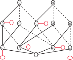
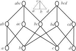
(a) (b)

Figure 9.7: Hasse diagrams and tries: the Hasse diagram for the lattice of faces of the two triangles $abc$, $bcd$ from Figure A.1 (b) and the corresponding trie (a) (see Example 9.5.16)

Example 9.5.16.

Consider for instance a set of words $W$ over the vocabulary $V=\{a,b,c,d\}$. Let be $W=\{a,ab,ac,abc,b,bc,bd,bcd,c,cd,d\}$. The corresponding trie ${\rm trie}(W)$ is shown in Figure 9.7a The red nodes consume an empty word and the dashed lines must be ignored and are there for future reference.

Tries can be implemented using a map for each node in the tree ${\rm trie}(W)$. Each map can be implemented as a binary search trees (BST). This kind of data structure was proposed in [8, 29] under the name of ternary search tree. In a ${\rm trie}(W)$, implemented with a ternary search tree, we can decide whether $\omega\in W$ or access information indexed by $\omega$ or insert a key $\omega$ with $\Theta(\log{|W|})$ comparisons (see Theorem 5 in [8]).

Each BST in a trie node can be heapified and represented with an array with no extra space. This array representation for each heap can be packed within a single array. For each map we propose to store a heapified BST. This could take at least, $\log{|V|}$ bits for each symbol to be consumed and $\log{N}$ bits to store and index for the next node to go. Here $N$ is the number of nodes in the tree. It can be proven that this minimal occupation can be attained (See references in section 9.3.5) With this convention the lenght of the array representation for all BST is easily available. Each node in the trie is reached from just one path and therefore we can implement the trie ${\rm trie}(W)$ using at most $\log{|V|}+\log{N}$ bits for each node in the tree ${\rm trie}(W)$. We note that this space is used to build the indexing data structure for the tree ${\rm trie}(W)$ and we still have to add the space for the information associated to each word in $W$.

Tries and Complexes

It is easy to associate a set of words, $W(\Omega)$ to an abstract simplicial complex $\Omega$ with Vertices in $V^{\prime}$. We just have to take for each simplex $\gamma=\{v_{j}|j=1,\ldots,n\}$ the word $\omega(\gamma)={<\!v_{p_{1}},\dots,v_{p_{n}}\!\!>}$ being $p_{i}$ the permutation of ${1\ldots n}$. such that $v_{p_{i}}>v_{p_{i+1}}$ in the (now ordered) set $V$. Thus we can associate a set of words $W(\Omega)$ to an abstract simplicial complex $\Omega$ given by $W(\Omega)=\{\omega(\gamma)|\gamma\in\Omega\}$. Similarly we can associate the trie ${\rm trie}(W(\Omega))$ to the abstract simplicial complex $\Omega$.

We note there is a tight relation between the abstract simplicial complex $\Omega$ and the associated trie ${\rm trie}(W(\Omega))$. In fact it can be proved that the Hasse diagram for the lattice associated with $\Omega$ contains (an isomorphic copy of) the forest of trees obtained from the trie ${\rm trie}(W(\Omega))$ deleting the root and all leaves consuming an empty word. For this reason we will reserve a special notation to this forest and we will denote it as ${\rm trie}(\Omega)$.

It can be proved that the forest ${\rm trie}(\Omega)$ spans completely the Hasse diagram, i.e. ${\rm trie}(\Omega)$ contains all Vertices in the Hasse diagram. The proof of this property builds upon the fact the forest obtained deleting the root from the trie subtree ${\rm trie}(W(\Omega)/v)$ is a forest that is (isomorphic to) a subgraph within the Hasse diagram for $lk(v)$. This forest spans completely the Hasse diagram for $lk(v)$, too.

Example 9.5.17.

Consider for instance the complex $\Omega$ made up of two adjacent triangles $abc$ and $bcd$ in Figure 9.7b. The corresponding set of words $W(\Omega)$ is $\{a,ab,ac,abc,b,bc,bd,bcd,c,cd,d\}$ and the corresponding ${\rm trie}(\Omega)$ is shown in Figure 9.7a. In Figure 9.7b we have the Hasse diagram for the lattice of the set of faces in an abstract simplicial complex $\Omega$ ordered by the face relation (see Definition 3.2.1). This is well known poset called the face lattice (see Example A.2.2). Looking at the two figures is easy to see that the ${\rm trie}(W(\Omega))$ is contained in the face lattice, just delete the red nodes, the root and add dashed lines.

This happens in general for every abstract simplicial complex. This claims is proven in the following property

Property 9.5.9.

Let $\Omega$ an abstract simplicial complexwith Vertices in $V$ with $|V|>1$. An isomorphic copy of a forest contained in ${\rm trie}(\Omega)$ is contained in the lattice induced by the poset of simplices of $\Omega$ ordered by the face relation. This forest spans completely all elements of the poset for $\Omega$. For each vertex $v$ in $\Omega$ we have that the forest obtained deleting the root and leaves from the ${\rm trie}(W(\Omega)/v)$ is isomorphic to a forest within the lattice for $lk(v)$. This forest spans completely all elements of the poset for $lk(v)$.

Proof 9.5.18.

The proof comes easily by induction of the number $|V|$ of Vertices in $\Omega$. If $|V|=1$ we have $\Omega={\{\{a\}\}}$ and both ${\rm trie}(\Omega)$ and the Hasse diagram for the face lattice are isomorphic, with just one node.

For the case $|V|>1$ we first note that the face lattice associated to $\Omega$ is a geometric lattice (see [31] §IV.11) whose minimal elements are vertices and whose maximal elements are top simplices. Directly from the definition of link we can say that the lattice for $lk({v},{\Omega})$ is isomorphic to a sublattice of $\Omega$ that contains the set of simplices $\gamma$ such that $v\in\gamma$. Thus, for each forest $F$ contained in the lattice for $lk({v},{\Omega})$, whose roots are minimal elements in $lk({v},{\Omega})$, we can find, in the lattice for $\Omega$ a tree rooted at $v$ and whose elements of depth $1$ are roots of the forest $F$.

Next we note that ${W(\Omega)/v}$ is exactly ${W(lk({v},{\Omega}))}$ and thus by inductive hypothesis deleting the root from ${\rm trie}(W(\Omega)/v)$ and empty leaves we obtain a forest within the Hasse diagram for $lk({v},{\Omega})$ that spans all nodes in $lk({v},{\Omega})$. Thus ${\rm trie}(W(\Omega)/v)$ is a tree within the lattice for $\Omega$. By the trie definition, deleting the root in ${\rm trie}(W(\Omega))$, we obtain a forest whose trees are the trees ${\rm trie}(W(\Omega)/v)$, one for each vertex $v$. Thus an isomorphic copy of the forest ${\rm trie}(\Omega)$ is contained in the lattice $\Omega$. We note that for all $v\in V$ the set of words ${W(\Omega)/v}$ is non-empty therefore we span all nodes in the lattice for $\Omega$.

We note that different forests ${\rm trie}(\Omega)$ are generated changing the ordering of $V$. However a particular forest, in general, is a proper subgraph of the Hasse diagram of the lattice $\Omega$ simply because some edges are missing. In general the tree ${\rm trie}(\Omega)$ contains all and alone the paths in the lattice for simplex $\gamma$.

Trie implementation

The implementation of this trie provide easily a data structure for the collective implementation of maps $V^{m}T$ for $0\leq m<d$. We just have to link information for $V^{m}T(\gamma)$ to the leaf node indexed by $\omega(\gamma)$. Similarly the map $\sigma_{\nabla}$ and each map indexed by $\sigma_{\nabla}(\gamma)$ can be implemented using a trie.

Tries can be implemented using binary search trees (BST) that in turn can be maintained as a complete binary trees and implemented by an heap using arrays using just one index for each node in the tree. If we assume this fact we can prove the following.

Property 9.5.10.

1. The construction of a collective trie for $V^{m}T$ for $0\leq m<d$ can be done with a time complexity of $O(|\Omega^{d-1}|\log{|\Omega^{d-1}|})$. where $|\Omega^{d-1}|$ is the number of simplices in the $d-1$ skeleton $\Omega^{d-1}$.

2. The the access time to $V^{m}T(\gamma)$ is $O(\log{f_{m}})$.

Proof 9.5.19.

To prove 1 we proceed as follows. The construction of $V^{m}T$ proceeds by inserting one after one all the words $\omega(\gamma)$ one for each $m$ simplex $\gamma$. Each insertion takes $m+1$ access to $m+1$ BST down the trie tree. Each access can be done in $\Theta(\log{s_{k}})$ where $s_{k}$ is the number of sons of the $k$-th node in the trie path we are following for insertion. The total access time is $\Theta(\log{s_{1}s_{2}\ldots s_{m+1}})$. Obviously the product ${s_{1}s_{2}\ldots s_{m+1}}$ is smaller than the number of leaves in the trie for $V^{m}T$. The number of leaves in the trie for $V^{m}T$ must be smaller than the face number $f_{m}$ of $m$-simplices in $\Omega$. Therefore the construction of the trie for $V^{m}T$ takes $O(f_{m}\log{f_{m}})$ and the construction of a collective trie for $V^{m}T$ for $0\leq m<d$ takes $O(|\Omega^{d-1}|\log{|\Omega^{d-1}|})$. where $|\Omega^{d-1}|$ is the total number of all simplices (not only top simplices) in the $d-1$ skelton $\Omega^{d-1}$.

Similar arguments can be used to prove Part 2. In fact the mechanism used to insert $\gamma$ is used also to access $V^{m}T(\gamma)$. Therefore the access to $V^{m}T(\gamma)$ takes $O(\log{f_{m}})$ even if a single trie is used to implement collectively all the $V^{m}T$ for $0\leq m<d$.

To analyze space requirements for this trie we assume that the BST is implemented using heaps. This choice do not change access time that remains logarithmic. With this implementation each BST in each trie node is maintained as complete binary tree. Thus it can be represented with an array with just one index for each node in the tree. Thus the number of indexes needed is just the number of nodes in the trie minus one. With this assumption we can prove the following

Property 9.5.11.

The construction of a collective trie for $V^{m}T$ for $0\leq m<d$ takes less than $|\Omega^{d-1}|(\log{|\Omega^{d-1}|}+\log{|V|}+\log{NT})$ bits.

Proof 9.5.20.

Now, due to the relation between the trie ${\rm trie}(\Omega)$ and the lattice for $\Omega$, expressed by Property 9.5.9, we can say that the number of nodes in ${\rm trie}(\Omega)$ is exactly $|\Omega^{d-1}|$. Therefore each index will take $\log{|\Omega^{d-1}|}$ bits and the whole indexing structure will take $|\Omega^{d-1}|(\log{|\Omega^{d-1}|}+\log{|V|})$.

Next we need to evaluate the space needed to reference a top simplex for each node in the trie for ${\rm trie}(\Omega)$. We have that each node $n$ in the trie corresponds to a simplex $\gamma(n)$ and must point a top simplex in $star({\gamma},{\Omega})$. Actually, we can reduce the number of these references to top simplices. We need only to associate top simplices to leaves of the trie tree. Infact when we reach $n(\gamma)$ we can still travel the tree to a leaf successor of $n$ and find a top simplex $\theta$ referenced by that leaf. This successor will be associated to a coface of $\gamma$ and therefore the top simplex $\theta$ must be incident to $\gamma$, too. Note that the leaves associated to $(d-1)$-simplices are not all the leaves of the tree ${\rm trie}(\Omega)$ and there are leaves that are associated to non-top simplices in $\Omega$. Thus these references will be coded with less than $|\Omega^{d-1}|\log{NT}$ Summing the two terms we obtain the thesis

Finally note that we do not need to insert in the trie ${\rm trie}(\Omega)$ the simplices that are already in the domain of $\sigma_{\nabla}$. These simplices will never be used as keys to access $V^{m}T$. Thus we can save in the implementation of the trie for ${\rm trie}(\Omega)$ the space needed for the indexing structure of $\sigma_{\nabla}$. The following property evaluates the space needed to code the elements in the codomain of the map $\sigma_{\nabla}$.

Property 9.5.12.

All the elements of the form $\sigma_{\nabla}[\gamma]$ can be encoded using less than $\phi(d\cdot\log{d\cdot\phi}+\log{NT^{\prime}})$ bits where $\phi=(2^{d+1}-(d+3))NSP$ and with $NSP$ we denote with $NSP$ the number of top simplices in the $d$-complex that are incident at least to a non-manifold simplex.

Proof 9.5.21.

We need to count the number of references to top simplices in the maps of the form $\sigma_{\nabla}[\gamma]$. The non-manifold simplices and the simplex copies in $\nabla\cdot{\Omega}$ maps to a subset of the non-manifold simplices in $\Omega$. Therefore simplices referenced by the map $\sigma_{\nabla}$ are simplices that are incident to a non-manifold simplex in $\Omega$. There cannot be, in the $\sigma_{\nabla}$ map, more references to a certain top simplex $\theta$ than the number of its $m$-faces, for $0<m<d$. In fact, if for the same simplex $\gamma^{\prime}$ in $\nabla\cdot{\Omega}$ we have non empty entries in $\sigma_{\nabla}[\gamma][\gamma^{\prime}]$ and $\sigma_{\nabla}[\beta][\gamma^{\prime}]$ must be $\gamma=\beta$. The overall number of $m$-faces for for $0<m<d$ is exactly $(2^{d+1}-(d+3))$. Thus there are at most $\phi=(2^{d+1}-(d+3))NSP$ references to top simplices in $\sigma_{\nabla}$. Considering that each reference to a top simplex takes $\log{NT^{\prime}}$ bits we need $\phi\log{NT^{\prime}}$ for all these references. Assuming the worst case of a tree with a distinct chain of maximum length for each reference we have $d\phi$ nodes and $d\log{d\phi}$ bits for each reference. This leads to $\phi d\log{d\phi}$ bits for the whole indexing structure of this trie. Summing the two terms we get the thesis.

We note that this is not a rough estimate of the space requested by this structure. It is quite easy to find a non-manifold for which the standard decomposition generates exactly $\phi=(2^{d+1}-(d+3))NSP$ simplex copies. We present this situation in the next example.

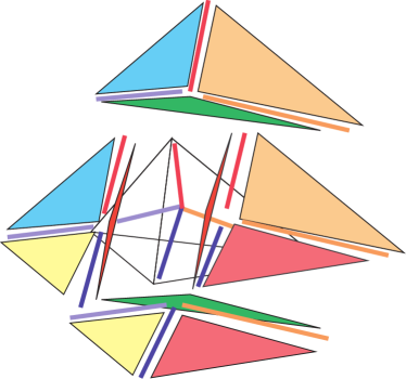
Figure 9.8: A 2-complex whose standard decomposition is totally exploded, see Example 9.5.22

Example 9.5.22.

The simplest example is given for $d=2$ by the $2$-skeleton of the tetrahedralization obtained by starring the standard $3$-simplex at some internal point. See Figure 9.8. The four transparent traingles defines the initial tetrahedron. This starring will split the $3$-simplex into a $3$-complex with $4$ tetrahedra. The $2$-skeleton of this complex has $10$ triangles. In Figure each new triangle is represented thrice with the same color. They are six. The triangles of the original tetrahedron are transparent and represented only once. The $2$-skeleton has $10$ edges. Each edge is a non-manifold edge. Indeed all edges are adjacent to three triangles. We represented internal edges with thick colored lines, four copies for each. Edges of the original tetrahedron are thin and black. Each is represented once. Thus each triangle is incident to a non-manifold edge. Thus for this complex we have $NSP=10$ and $d=2$ and therefore $\phi=30$. The standard decomposition of this complex is its totally exploded version with $10$ distinct triangles. Thus we have $30$ $1$-simplex copies.

9.6 Summary and Discussion

In this section we recall the proposed representation and the associated date structure. We summarize space and time performance and compare space requirements with existing solutions.

The Non-manifold Winged Representation (see Definition 9.5.1) and the associated Data Structure (see Data Structure 9.5.1) NMWDS=(EWS,$\sigma$,$\sigma^{-1}$,$\sigma_{\nabla}$) can encode a $d$-complex $\Omega$ encoding its standard decomposition $\nabla\cdot{\Omega}$. This representation is a two layer representation. In the lower layer we encode the connected components of the complex $\nabla\cdot{\Omega}$ using the Extended Winged Representation ($EWS$ ) (see Definition 9.4.2). The associated Data Structure (see Data Structure 9.4.1) is extended to a Global Extended Winged Data Structure (see Data Structure 9.5.2) to accommodate, in the single data structure $EWS$, the decomposition $\nabla\cdot{\Omega}$. This data structure is then optimized to the the more compressed Implicit Data Structure B.0.2.

On the other hand, the upper layer is made up of the two relations $\nabla$ and ${\geq^{\nabla}}^{\star}$ implemented by the three maps: $\sigma$,$\sigma^{-1}$ (see Section 9.5.3) and $\sigma_{\nabla}$ (see Section 9.5.4).

9.6.1 Space Requirements

If the original complex has $NV$ vertices and $NT$ top simplices and if we denote with $NS$ the number of splitting vertices and with $NC$ the number of vertex copies introduced by the decomposition process we have that the encoding of $\nabla\cdot{\Omega}$ takes (see Property 9.5.1)

$${\rm SIZE}(\log{NT^{\prime}}+\log{NV^{\prime}})+NV^{\prime}\log{NT^{\prime}}\,\mbox{\rm bits}$$

where: ${\rm SIZE}=\sum_{0\leq h\leq d}{|\Theta^{[h]}|(h+1)}$, being $\Theta^{[h]}$ the set of top $h$-simplices in $\Omega$. and $NV^{\prime}=NV-NS+NC$. This representation can be compressed saving (see Property B.0.1) $NV^{\prime}(\log{NV^{\prime}}+\log{NT^{\prime}})$ bits.

The upper layer, made up of the maps: $\sigma$,$\sigma^{-1}$ and $\sigma_{\nabla}$ takes:

1. up to $NS\log{NS}+NC\log{NC}$ bits to encode the map $\sigma^{-1}$ (see Property 9.5.2)

2. $NC(\log{NC}+\log{NS})$ bits to be encode the map $\sigma$ (see Property 9.5.2)

3. the map $\sigma_{\nabla}$ can be encoded using less than $\phi(d\log{d\phi}+\log{NT^{\prime}})$ bits where $\phi=(2^{d+1}-(d+3))NSP$ and where with $NSP$ we we denote the number of top simplices in the $d$-complex that are incident at least to a non-manifold simplex.(see Property 9.5.12)

9.6.2 Information and Non-Manifoldness

Note that the three parameters $NS$, $NSP$, $NC$ gives a measure of three different aspects of the non manifoldness in the complex $\Omega$: $NS$ gives an idea how how many singularities are present. $NSP$ gives an idea of which portion of the original complex is incident to non-manifold situations. $NC$ gives an idea of the severity of the non-manifoldness in terms of the complexity of the actions needed to split the complex into initial-quasi-manifold components. The results above shows that, for a complex with a certain number $NT^{\prime}$ of top simplices, the information needed to encode its singularities is an increasing function of these three parameters. Thus, this gives some theoretical foundation to a classification of the complexity of the non-manifold structure of a complex in term of the three parameters $NC$, $NS$ and $NSP$, using the information given by the formula:

$$\widehat{H(\Omega)}=NS\log{NS}+NC\log{NC}+\phi(d\log{d\phi}+\log{NT^{\prime}})$$ (9.14)

This formula is obtained summing the space needed by the map $\sigma$ and by the map $\sigma_{\nabla}$. We omit the map $\sigma^{-1}$ being clearly redundant w.r.t. $\sigma$. The analysis of our two layer data structure shows that the quantity $\widehat{H(\Omega)}$ in formula 9.14 is surely an upper bound for the information associated with the non-manifold aspects in a complex. This quantity, or a normalized version of it, can be used for the classification of non-manifold structures according to the complexity of their non-manifold structure.

.

9.6.3 Time Requirements for the Construction of the Non-manifold Winged Data Structure

We assumed that the map $\sigma$ is a by-product of the output of the decomposition algorithm that takes $O(NT\log{NT})$ (see 8.5.2). From this output we can build the NMWDS=(EWS,$\sigma$,$\sigma^{-1}$,$\sigma_{\nabla}$) data structure with the following time requirements:

• The EWS data structure can be built in $O(d^{2}NT\log{NT})$ (see Property 9.4.1) using Algorithm 9.4.1 and can be optimized using Algorithm 9.4.5 and Algorithms from B.0.1 to B.0.3. This optimization takes $O(dNT^{\prime})$ (see Property B.0.1);

• The map $\sigma$ comes from the decomposition process and the map $\sigma^{-1}$ can be build out of $\sigma$ in $\Theta(NC\log{NC})$ (See Property 9.5.2);

• The map $\sigma_{\nabla}$ can be computed using Algorithms 9.5.2 and 9.5.3 in $O(NSP\cdot 2^{d}\log{NSP})$ (See Property 9.5.4)

The complexity of $O(NSP\cdot 2^{d}\log{NSP})$ represent a drastic reduction in complexity w.r.t. a global analysis. This reduction is possible due to the prior decomposition of the original complex $\Omega$ that allows, when building $\sigma_{\nabla}$, to restrict the search to the neighborhood of a subset of non-manifold vertices.

9.6.4 Extraction of Topological relations $S_{nm}(\Omega,\gamma)$

The Non-manifold Winged Data Structure supports the computation of the topological relations $S_{nm}(\Omega,\gamma)$ using only the $\sigma$ and $\sigma^{-1}$ maps (see Formula 9.11 in Section 9.5.4). In particular, using Algorithm 9.5.1 we can compute $S_{0m}(\Omega,\gamma)$ in $O(n\log{n})$ being $n$ the size of the output. This holds for $2$-complexes and for $3$-complexes embeddable in ${\rm I\kern-1.99997ptR}^{3}$ (See Property 9.5.3). However, in general the complexity of the associated computation can become polynomial w.r.t. the dimension of the output (see Properties 9.2.5, 9.2.6 and 9.2.7). The computation of $S_{nm}(\Omega,\gamma)$ in $O(n\log{n})$ can be supported adding the $\sigma_{\nabla}$ relation. In this case, using Algorithm 9.5.6, we can compute $S_{nm}(\Omega,\gamma|\theta)$ in $O(n\log{n})$ being $n$ the size of the output and assuming that at least a top simplex $\theta$ incident to $\gamma$ is given at the beginning of the computation (see Property 9.5.8).

Finally the task of providing a top simplex incident to a given $n$-simplex $\gamma$ is carried through by an auxiliary data structure that we called the $V^{m}T$ amp. This data structure represents the way in which we introduce, in the framework of the Non-manifold Winged Representation, an explicit modeling for $m$-simplices for $1\leq m\leq d-1$.

The basic facts about the map $V^{m}T$ are the following:

• The construction of a collective trie for $V^{m}T$ for $0\leq m<d$ takes less than $|\Omega^{d-1}|(\log{|\Omega^{d-1}|}+\log{|V|}+\log{NT})$ bits (see Property 9.5.11) being $\Omega^{d-1}$ the $(d-1)$ skeleton of $\Omega$. Hence $|\Omega^{d-1}|=\sum_{0\leq k\leq(d-1)}f_{k}\log{f_{k}}$

• The construction of a collective data structure for $V^{m}T$ for $0\leq m<d$ can be done with a time complexity of $O(|\Omega^{d-1}|\log{|\Omega^{d-1}|})$. where $|\Omega^{d-1}|$ is the number of simplices in the $d-1$ skelton (See Property 9.5.10 Part 1)

• The the access time to $V^{m}T[\gamma]$ is $O(\log{f_{m}})$ (See Property 9.5.10 Part 2)

9.6.5 Comparison with existing approaches

For the comparison between manifold and non-manifold approaches we refer to the empirical study in [73] where classic non-manifold modeling schemes are compared with classical manifold modeling approaches such as the Winged Edge [12] and the Half Edge [86]. This empirical analysis was conducted on the ground of statistical data from [135] for solid models represented by cellular complexes. The results shown in Figure 9.9 (but row 4) are reported in [73]. They give some ratios for known modeling approaches for non-manifold surfaces:

Figure 9.9: Space requirements for different data structures for surfaces normalized vs. space requirements for the Half Edge. Data (but the fourth row) are from [73]

Modeling Data Structure		Ratio to HE
Half Edge		1
1	Winged Edge	0.80
2	Partial Edge	1.7
3	Radial Edge	3.5
4	EWDS	0.92

The fourth row is theoretically computed assuming a manifold triangulated closed surface of genus $0$. This ratio comes from the fact that the Non-manifold Winged Data Structure reduces to the Extended Winged Data Structure for manifold objects and we have seen that an optimized Global Extended Winged Data Structure uses 5.5 pointers for each triangle (see remark at the end of Property B.0.1). Thus we have that for the Extended Winged Data Structure the ratio to the Half Edge is $5.5/6=0.92$ since the Half Edge uses six pointers for each triangle.

If we add an explicit representation for edges we must add $f_{1}$ pointers for edges plus $f_{0}+f_{1}$ pointers for the indexing structure of $V^{1}T$ yielding additional 3.5 pointers for each triangle. In this case the ratio to the Half Edge rise to $9/6=1.5$. However note that neither the Half Edge nor the Winged Edge offer an explicit representation for vertices and faces since they are based on explicit modeling for edges. On the other hand, the Extended Winged Data Structure is based on the explicit representation of triangles and vertices.

We next compare the Extended Winged with approaches for manifold volumetric cellular representations [57, 81]. In the Handle-Face Data Structure [81] we have 36 pointers for each tetrahedron for a occupancy of $36f_{3}$ while in the Facet-Edge Data Structure [57] we have a data structure requiring $12f_{2}$ pointers. These two approaches compares with ${\rm SIZE}(\log{NT^{\prime}}+\log{NV^{\prime}})-NV^{\prime}\log{NV^{\prime}}$ bits where ${\rm SIZE}=4f_{3}$. If we assume that $\log{NT^{\prime}}$ and $\log{NV^{\prime}}$ are replaced by the size of a pointer we got an occupancy of $8f_{3}-f_{0}$ pointers. Adding an explicit representation for edges and triangles we have to add the maps $V^{1}T$ and $V^{2}T$. Thus we need $f_{0}+2f_{1}+2f_{2}$ pointers for a total of $o=8f_{3}+2f_{1}+2f_{2}$ pointers. Since we are comparing the occupancy for manifold models we have from Property 9.2.1 $4f_{3}\leq 2f_{2}$ and using the fact that in a tetrahedralization $f_{0}\leq 4f_{3}$, $f_{1}\leq 6f_{3}$ and $f_{2}\leq 4f_{3}$ we have that $o\leq 28f_{3}$. This shows that the ratio with the Handle-Face is above $36/28=1.28$ using also Property 9.2.3 $4f_{3}-3f_{2}+2f_{1}=2f_{0}$ it is easy to see that $o=4f_{3}+5f_{2}+2f_{0}\leq 12f_{3}+5f_{2}\leq 11f_{2}$. This shows that the ratio with the Facet-Edge is above $12/11=1.09$.

A comparison is possible also with models based on incidence graph. These [53, 136] encodes completely the lattice associated with the complex $\Omega$ with using two pointers to represent each edge in the Hasse Diagram for $\Omega$. This requires, for a tetrahedralization $2(4f_{3}+3f_{2}+2f_{1})$ pointers. relations. A reduced scheme can reach the occupancy of at most $8f_{3}+3f_{2}+3f_{1}+f_{0}$. This is above the occupancy of the Non-manifold Winged (i.e. $o=8f_{3}+2f_{1}+2f_{2}$) of a difference of $f_{2}+f_{1}+f_{0}$. It is easy to see that the ratio vs. this reduced version of incidence graph is above $1.07$. Finally in Brissons’s Cell Tuple [22] and in Lienhardt’s n-G-maps [78] the representation is $\Theta(df_{d}(d+1)!)$ while the Extended Winged, enriched with $V^{d-1}T$, occupies $O(f_{d}2^{d})$ thus the ratio between the two is $O(2^{d}/d(d+1)!)$ that asymptotically tends to zero. For $d=3$ We have a ratio w.r.t. the Cell Tuple that is above $3.43$ and the ratio w.r.t the n-G-maps is above $2,57$. The following table summarize this analysis and gives the relation between the Extended Winged Data structure and other modeling approaches compared over the domain of tetrahedralizations of $3$-manifolds.

Figure 9.10: Space requirements for different data structure for $d$-manifolds for $d\geq 3$ normalized v.s. space requirements for Non-manifold Winged Data Structure

Modeling Data Structure		Ratio to EWDS
EWDS		1
1	Handle-Face	$>1.28$
2	Facet-Edge	$>1.09$
3	Incidence Graph	$>1.07$
4	Cell Tuple	3.43
5	n-G-map	2.57

Obviously this comparison do not take into account the fact that these approaches can model cellular complexes and thus the comparison might be not so bright in all those cases in which if the applicative domain do not impose a simplicial representation. Nevertheless our scheme is compact enough to encode manifold surfaces and manifold tetrahedralizations, providing explicit representation for all $n$-simplices being always more compact than classic approaches in the field.

When we apply this approach to model non-manifold complexes the space requirements of our data structure grows linearly with the structural complexity of non-manifoldness in the modeled complex. This data structure is useful as long as the structural complexity of non-manifoldness is not too deep. Otherwise the size of auxiliary structures used to model non-manifoldness might be too important and probaly a data structure conceived to model non-manifoldness everywhere is a better modeling choice. To give a rough estimate of the tradeoff between this approach and the other approaches we restrict out attention to regular non-manifold complexes. We rework the formula that gives the occupancy of the upper layer i.e. the sum of the three terms

$$NS\log{NS}+NC\log{NC};\,NC(\log{NC}+\log{NS});\,{\phi(d\log{d\phi}+\log{NT^{\prime}})}$$

where $\phi=(2^{d+1}-(d+3))NSP$ and where with $NSP$ we we denote the number of top simplices in the $d$-complex that are incident at least to a non-manifold simplex.(see Property 9.5.12); with $NS$ we denote the number of splitting vertices and with $NC$ the number of vertex copies introduced by the decomposition process. We can assume that all logarithmic terms in formulas above are replaced by the size of a pointer. Then we use the fact that $NS<NSP$ and $NC<NSP$ to see that less than $(\phi(d+1)+4)NSP$ pointers are necessary to encode the upper layer. For $d=2$ we have to add at most $13$ pointers for each triangle incident to a non manifold vertex. For $d=3$ 40 more pointers are needed.

Using data from table in Figure 9.9 and restricting our attention to regular 2-complexes we can predict that 21 pointers per triangle are needed by the Radial Edge and 10.2 pointers per triangle are needed by the Partial Edge Data Structure. We ask for 5.5 pointers for triangle to encode the decomposition and 9 pointers for triangle to encode the decomposition modeling explicitly all simplices. w.r.t. the Radial Edge we use from 15.5 to 12 pointers less for each triangle and this gain is balanced when $13NSP=12f_{2}$ thus our representation is a viable substitute for the Radial Edge when the ratio $NSP/f_{2}$ is below $12/13=0.92$.

Thus as long as the number of non-manifold triangles adjacent to a non-manifold simplex is less than the 92% we have some profit in using our data structure instead of the Radial Edge. Furthermore our solution is always preferable if we do not need to model all simplices and thus we do not introduce $V^{2}T$.

The same comparison for the Partial Edge yields an interval from 13% to 40%. Namely if $NSP/f_{2}$ is below 13% we can save space using our data structure instead of the Partial Entity Data Structure. If we do not need the $V^{2}T$ relation we can use our data structure whenever $NSP/f_{2}$ is below 40%.

For regular $3$-complexes the most relevant modeling option to compare with is the Incidence Graph. The Incidence Graph data structure requires $8f_{3}+6f_{2}+4f_{1}$ relations to be stored. Since the lower layer takes $o=8f_{3}+2f_{1}+2f_{2}$ pointers we remain with a gain of $4f_{2}+2f_{1}$ pointers that are used by the upper layer. Obviously in this case we consider a data structure containing $V^{1}T$ and $V^{2}T$ because all simplices are explicitly modeled by the Incidence Graph. The upper layer takes less than $40NSP$ pointers and this equates the gain of $4f_{2}+2f_{1}$ when $NSP/f_{3}$ is the limit ratio $NSP/f_{3}=(4f_{2}+2f_{1})/40f_{3}$. If we assume that we are dealing with complexes imbeddable in ${\rm I\kern-1.99997ptR}^{3}$ we have $4f_{3}\leq 2f_{2}$ and thus the limit ratio is always bigger than $8f_{3}+2f_{1}/40f_{3}\geq 1/5$. Thus in this case our data structure is a more efficient option than Incidence Graph whenever $NSP/f_{3}$ is below 20%.

Chapter 10 Conclusions

In this short chapter we recall briefly several proposals from the state-of-the-art in Chapter 2 and show how the results in this thesis represent a (possibly) relevant option w.r.t. existing solutions.

10.1 The decomposition problem

In the first part of this thesis we studied the problem of decomposing a generic non– manifold simplicial d- complex into more regular components [36]. We called these components initial-quasi-manifold. This problem was considered in the context of Combinatorial Topology and the results obtained are dimension independent. This first part provided a better understanding of the combinatorial structure of non-manifolds and represents a contribution in the direction of topology-based geometric modeling [79]. The problem of decomposing non-manifolds has been already studied in geometric modeling. However, the few proposed solutions [37, 46, 114] are limited to the problem of decomposing surfaces. In particular, in [46] the problem of decomposing two-dimensional boundary representations of r-sets (i.e., uniformly two-dimensional objects) is studied. In [37] this former decomposition of the boundary of r-sets is assumed and extended Euler operators are introduced to build such a model. Finally, in [114] is presented an algorithm, called Matchmaker, that decomposes the boundary of r-sets (or even a 2-complex) into a set of manifold surfaces. This latter approach, although restricted to non-manifold 2-complexes, attempts to minimize the number of duplications introduced by the decomposition process. In [56, 55] we also find the idea of cutting a two-dimensional non-manifold complex into manifold pieces. This decomposition is used within a geometric compression algorithm that uses a two level representation: in a first level manifold components are encoded separately, the second level encodes stitching instructions for components. From the very beginning of our study we have noticed that the decomposition of a complex could be studied with no reference to the geometry of the complex and, thus, we adopted the classical framework of the Combinatorial Topology [52, 25]. Indeed, a strong relation between Combinatorial Topology and Topology based Geometric Modeling is clearly pointed out in [79]. A major benefit of this (purely combinatorial) approach is the possibility of treating the general problem of decomposition in any dimension. A second benefit is the possibility of providing proofs that do not require geometric intuition.

10.2 Decomposition: a formal definition

In this framework we first tackled the problem of giving a non-operational definition of the notion of decomposition. A naive statement of the decomposition problem might require to search for a decomposition algorithm that decompose a complex into maximal manifold connected components. By requiring maximal components, we mean that we do not accept decomposition where there are components that can be merged into a bigger manifold subcomplex. This requirement about maximal components seems quite ”natural” since, otherwise, the problem becomes quite trivial and the collection of all top simplices in the original complex, each considered as separate component, would be a solution to this problem. A first result (that it is quite easy to prove) was that the decomposition problem, with such a requirement about maximal manifold components, is, in general, unsolvable. Classical results in combinatorial topology [88, 125] easily imply that, for $d\geq 6$, there is not a decomposition algorithm that splits a generic d-complex into maximal manifold parts. Such a decomposition problem is actually equivalent to recognizability of d-manifolds. This problem is settled for $d=4$ [123], it is still an open problem for $d=5$ and is known to be unsolvable for $d\geq 6$ [125]. Moreover, already for surfaces, several possible decompositions exists. The non-uniquiness of decomposition is usually neglected in existing approaches (with the notable exception of [114]).

We have defined a decomposition using a specific class of abstract simplicial maps and using the notion of combinatorial manifold. Intuitively we can say that we have chosen to define a decomposition as the result of a process that is allowed to cut a complex just along singular (non-manifold) features. We have found that this statement, although apparently ”natural”, has some important consequences. First of all, there are 3-complexes that cannot be decomposed into manifold parts. It is interesting to note that some of those unbreakable tetrahedralizations fell into the class of non-manifolds defined by Lienhardt and called quasi-manifold [80]. However we have found examples of 3–complexes that cannot be decomposed into pseudomanifolds. Equivalently we can find examples of non-pseudomanifold tetrahedralizations that cannot be decomposed (according to the decomposition notion given above) into pseudomanifold parts. This means that there are certain tetrahedralizations that cannot decomposed into pseudomanifold components by simply cutting them at singular features. An example of such a tetrahedralization is given in the thesis.

A possible solution is to break the unbreakable complex along non singular features. This is clearly not desirable since several arbitrary cuts are possible. There are examples of unbreakable tetrahedralizations where different cuts, along non singular features, will yield alternative non homeomorphic decompositions.

This problem of choosing among several possible decomposition is not addressed too often in existing literature. The best answer to the possible impasse in choosing is in Matchmaker [114]. Matchmaker is a decomposition algorithm for surfaces that searches the space of possible decomposition by looking for an optimal solution according to some a priori criterion. Another finding in this thesis is that there exist always a most general decomposition and all the others proposed solutions are options taking some more stitching for components that are separated in the most general solution.

10.3 The Standard Decomposition

Indeed, our goal was to see if it could be possible to define a non-arbitrary non a priori decomposition. We assumed that a non arbitrary decomposition must be, somehow, more general than other decomposition. Intuitively, we look for a decomposition obtained by further cuts in other arbitrary decomposition. We search the decomposition space for a general solution by cutting arbitrary decomposition. In this search, we forbid to cut along features that were manifold (i.e. non-singular) in the original complex. In other words, we ask to cut as much as possible whenever we cut at a singular features and see if a most general decomposition exist. One of the main results of this first theoretical part is that such a decomposition exists for a generic d-complex. Furthermore, we have proven that, for any d, this decomposition is unique up to isomorphism. We called such a decomposition the Standard Decomposition. In spite of the fact that a decomposition into manifolds is not computable, we have found that the standard decomposition can be computed. If $t$ is the number of top simplices in the standard decomposition, this computation can be done at least in (nearly) linear time (i.e. $\Theta(t\log{t})$ ). We have developed an algorithm that transforms a complex into its standard decomposition by a sequence of local operations modifying just simplices which are incident at a vertex. Each local operation is computed using just local information about the star of the vertex (i.e., the set of simplices incident to a vertex).

10.4 The Decomposition Lattice and Initial-Quasi-Manifolds

To provide a framework for the results of this first part of the thesis we have defined an ordering among complexes and built a poset. This poset orders all the possible modifications for a complex. Possible modifications we considered are those obtained by a sequence of vertex pair stitching (a vertex pair stitching being the transformation that collapses together two vertices). This poset turns out to be a lattice with a top and a bottom element. The top element is the complex made up of a set of isolated simplices and the bottom element is the complex made up of a single point. Every complex in this lattice is associated with an equivalence relation between vertices. One can move on the lattice adding equations that stitch together just two vertices at time. In this framework the standard decomposition becomes simply the least upper bound for a specific set of decompositions, obtained by cutting a complex at singularities.

Although this lattice originates from the particular goal of studying decompositions we think that this construction can be useful in general. This framework supports the study of topological properties of complexes by tracing syntactical properties of sets of equations between vertices. Using equations, we have analyzed the topological property of the connected components in standard decomposition. We singled out the class of complexes that are possible connected components in a standard decomposition. We called these complexes initial-quasi-manifolds. It is an easy consequence of this theoretical development that initial-quasi-manifold are all and alone the unbreakable complexes. Thus, the standard decomposition of an initial-quasi-manifold complex is the complex itself.

We have proven that initial-quasi-manifold can be defined in terms of local properties of the star of each vertex. In the star of an initial-quasi-manifold two top d-simplices must be connected with a path of d-simplices, each linked to the other via a (d-1)-manifold (non singular) joint. It can be proven that initial-quasi-manifold d-complexes are a proper superset of d-manifolds for $d\geq 3$. They coincide with manifolds for $d=2$. Furthermore, it is easy to see that initial-quasi-manifolds are a decidable set of d-complexes for any d. As we already mentioned, there are (initial-quasi-manifold) tetrahedralizations that are unbreakable and that are not pseudomanifold. However, such a tetrahedralization cannot be embedded in ${\rm I\kern-1.99997ptR}^{3}$ . We like to mention that a nice benefit of this theoretical framework has been the possibility of checking a proof of the correctness of this example, that we cannot visualize, by manipulating equations via a Prolog program.

Furthermore, we felt that the methodology and notations developed for this part can be used to give a set of algebraic tools that can be used to study other application domains in Computer Graphics such as: Simplification, Compression, Multi-resolution and Feature based classification. According to this strong feeling we found interesting to develop this study within a formal settlement as an example of how algebraic techniques and combinatorics can be used for this task.

10.5 The Non-Manifold Data Structure

The second part of this thesis dealt with a two layered data structure conceived to model the decomposed non-manifold. This data structure models separately the structure of the decomposition and each connected component of the decomposition. The decomposition structure, at an abstract level, is modeled via an hypergraph [35]. Each component of the decomposition is encoded using an extended version of the Winged Representation [103]. This approach offered a compact, dimension independent, data structure for non-manifolds that can be used whenever the modeled object has few non-manifold singularities. Algorithms used to build and navigate this data structure were presented. We have shown that they have optimal time performance in the usual domain of 2-complexes and 3-complexes. We also analyzed the space requirements of the two layer data structure and discussed a possible approach for the computation of all topological relations.

Most common data structures for non-manifolds [130, 59, 73] are quite space-consuming since they assume that non-manifoldness can occur very often in the model. The resulting data structures are designed to accommodate a singularity everywhere in the modeled object. As a result, storage costs do not scale with the number of non-manifold singularities. In other words, the performance of such non-manifold data structure is quite poor when used to code a manifold. On the other hand, very efficient data structures for subdivided 2-manifolds [12, 86, 81, 58, 57] do exist. Furthermore, most modeling proposals for non–manifolds are limited to 2-complexes and the few data structures for dimension independent modeling do not pay special attention to singularities. Some of them code just manifolds [22], or a special subset of non-manifolds [80]. Others are quite general since they simply code incidence relations between cells [53] or a subset of these incidence relations [136, 34]. Models based on incidence relations can be quite satisfactory, supporting even a full set of Boolean operations [112]. However. in general, models encoding incidence relations between cells can be quite space consuming if simple cells (e.g. triangles) are used. On the contrary, models based on incidence relations can be quite compact provided that one decompose the object into few components and a single cell is used for each component. Obviously, to have a compact model, a compact coding scheme for each component must exist. Thus we studied the problem of representing a simplicial d-complex using our the decomposition into initial-quasi-manifold connected components.

10.5.1 The Two-Layer Data Structure

Having established a sound notion of decomposition, we have considered the design of a dimension independent layered data structure that exploits this decomposition. In this direction we have been influenced by the idea behind SGC [112] where complexes are modeled with a cellular complex with quite complex cells. In an SGC the cellular complex, represented via an incidence graph, can be regarded as an upper layer that ties together quite complex cells that can, for instance, be any open manifold merged in ${\rm I\kern-1.99997ptR}^{3}$.

For the data structure used to code initial-quasi-manifolds components, we see some relations with ideas in some works in the field of dimension independent modeling. In particular we were influenced by ideas of Lienhardt on nG-maps [78, 44] and somehow by Brissons’s cell-tuples [22]. All these approaches provide a dimension independent machinery to represent, respectively, either a certain subclass of non-manifold complexes or plain d-manifolds. Similarly we adopted a uniform, dimension independent, scheme to represent initial-quasi-manifold. This scheme is an extended version of the Winged Representation [103] and the modeled class of complexes (i.e. initial-quasi-manifold) is very close to Lienhardt’ s quasimanifold.

On the other hand the concept behind data structure we propose is, somehow, complementary to the Radial-Edge structure [130]. In our two-layer data structure the upper level is used to encode the structure of the decomposition. This is done by encoding an hypergraph [35]. From the results about the decomposition process we have that, in the decomposition process, just singular (i.e. non-manifold) simplices are duplicated across different components. Furthermore there is no need to represent explicitly sub-faces of a duplicated singular simplex. Hence, in this hypergraph, nodes contain the representation of initial-quasi-manifold components and hyperarcs need to encode just top singular simplices. In each hyperarc we store the description of non-manifold vertices for the corresponding top singular simplex. On the other hand, the lower level is devoted to the coding of (initial-quasi-manifold) decomposition components.

The coding of (initial-quasi-manifold) decomposition components is accomplished via an unconstrained usage of the the Winged Representation [103]. The Winged Representation considers complexes built stitching d-simplices at (d-1)-faces. This offers exactly the right level of abstraction to treat initial-quasi-manifold components. We point out that this scheme is used here beyond its intended domain in order to treat initial-quasi-manifolds that can be even non-pseudomanifolds.

To encode the hypergraph, some additional information must be added to the coding of singular vertices in each initial-quasi- manifold. We stress that this additional data need only to be provided for non-manifold vertices. Whenever the number of non-manifold vertices is low, this additional information can be stored and retrieved easily using hashing techniques.

We note that completeness of this data structure comes from the definition and the existence of standardized decompositions. Similarly uniqueness of representation comes from our result on uniqueness of the standardized decompositions.

Finally, in the last part of the thesis, the two layer data structure is developed in detail showing how we can construct this data structure using the results of the decomposition algorithm. The complexity of the proposed solution is analyzed. In particular, we detail space requirements and give the complexity required to build the data structure and to extract all topological relations between simplices of different dimension. The proposed two layer data structure proves to be fast and compact with respect to existing approaches.

Another interesting result in the second part of this thesis comes from a trivial application of deep results from Combinatorics. Data structures that stores only (d-1)-adjacency between top d-simplices are bound to travel all (d-1) simplices around a vertex to find all d-simplices incident to a certain vertex. This choice bounds extraction to be non optimal in higher dimension. The idea was to see what happens of this search scheme when going in higher dimension. We were interested in that because we adopted such a scheme to encode initial-quasi-manifold components for our decomposition. For $d\geq 4$ classical results in combinatorial topology (i.e. the so called Upper Bound Theorem by McMullen [84]) implies that extraction time of some topological relations could be non-optimal. More precisely (see Property 9.2.5 and 9.4.9) complexity is polynomial. For instance, finding all edges round a vertex is $\Theta(e^{\left\lfloor{d/2}\right\rfloor})$ where $e$ is the number of edges in the output.

Appendix A Posets, Lattices and the Partition Lattice

A.1 Introduction

In this thesis it is crucial to compare decompositions as generated by equivalences among vertices. The goal of this appendix is to introduce the right mathematical framework to order equivalences. Equivalences, ordered by set inclusion, form a partially ordered set that is a well known object in Lattice Theory. This lattice is called the Partition Lattice and is usually denoted by $\Pi_{n}$. In this appendix we summarize basic notions from Lattice Theory necessary to present the properties of the Partition Lattice. These properties, often recalled in this thesis by a claim to intuitive arguments, are used extensively. In this section intuition is left apart and we show that there is a mathematical framework behind this claim to intuition.

The last section of this appendix develops, is more specific to this thesis and specialize this notion to the aims of our work. The reader that might find hard to read the first three sections might browse directly to the last section to have an idea of what is this all about. The material reported here is not meant to be a self-contained presentation of this subject. Thus, some useful results are reported without proof. However precise reference to textbooks is given for each result. The interested reader may refer to [31, 83, 61] for a complete treatment.

A.2 Partially Ordered Sets (Poset)

A (binary) relation $R$ on a set $X$ is any subset of the cartesian product $X\times X$. We will write $xRy$ to mean $(x,y)\in R$. A relation $R$ is a reflexive relation if and only if  $xRx$ for all $x\in X$. The relation $\Delta_{X}=\{(x,x)|x\in X\}$, called the diagonal in $X$. The diagonal is the smallest reflexive relation on $X$. A relation $<$ is a transitive relation if and only if  for all $x$, $y$ and $z$ such that $x<y$ and $y<z$ we have that that $x<z$. A transitive and reflexive binary relation $x\leq y$ is called a preorder (see [83] Pg. 10). A relation $R$ is a symmetric relation if and only if  for all $x$, $y$ we have that $xRy$ implies $yRx$. A relation $R$ is a antisymmetric relation if and only if  for all $x$, $y$ we have that $xRy$ and $yRx$ implies that $x\equiv y$ (i.e. $x$ and $y$ are the same element in $X$). An antisymmetric preorder $x\leq y$ is called an ordering or a partial order on $X$. For a given ordering $\leq$ we will denote with $x<y$ the relation obtained deleting from $\leq$ all elements in the diagonal $\Delta_{X}$ (i.e. $x<y$ iff $x\leq y$ and $x\neq y$). If $\leq$ is an ordering on $X$ the set $X$ is called a partially ordered set and the pair $P={{<}{X},{\leq}{>}}$ is called a partially ordered set or poset. With some abuse of notation we will write $x\in P$ to mean $x\in X$. Finite posets can be represented by particular diagrams called Hasse diagrams. To define Hasse diagrams we need to introduce some more definitions.

Definition A.2.1 (Immediate Superior (see [31] Pg. 4)).

We will say that in a poset $P={{<}{X},{\leq}{>}}$ $x$ covers $y$ whenever $x>y$ and, for no $z\in X$, $x>z>y$. In this situation $x$ is called the immediate superior of $y$ in $P$.

Similarly $y$ is called the immediate inferior of $x$ in $P$. Using the covering relation one can represent a poset $P$ with a directed graph $G(P)$ such that $(x,y)$ is an edge in $G(P)$ if and only if  $x$ covers $y$. It can be proved that the graph $G(P)$ is an acyclic graph (see Lemma 2 Pg. 2 [31]) If we take the unoriented graph associated with $G(P)$ and we draw it with straght arcs placing $x$ above $y$ whenever $x$ covers $y$ we have what is called define the Hasse diagram for $P$.

Example A.2.2.

As an example of a poset and of its Hasse diagram consider the set of faces in an abstract simplicial complex $\Omega$ ordered by the face relation (see Definition 3.2.1). This is well known poset called the face lattice (see [50] Pg. 247). Figure A.1a shows the Hasse diagram for the face lattice for the triangle $abc$. Elements of this poset are all the faces of the triangle. Thus we have the three vertices, $a$, $b$ and $c$ and the three edges $ab$, $bc$, $ca$. The top element is the triangle itsself. In Figure A.1b we have the Hasse diagram for the complex made up of the two triangles $abc$ and $cbd$.

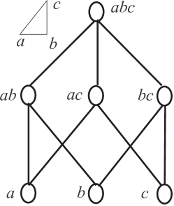
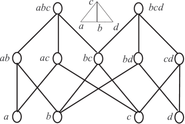
a b

Figure A.1: Two Hasse diagrams: the Hasse diagram of the face lattice for the triangle $abc$ (a) and the Hasse diagram for the two triangles $abc$, $bcd$

A classification of polytopes (see proof of Property 9.2.4 for a definition of polytope) can be given abstracting completely from geometry (see [19] Pg. 129 and [20]).

A partially ordered set where, for all $x,y\in X$, either $x\leq y$ or $y\leq x$ is called a totally ordered set or a linearly ordered set or a chain. Two elements $x,y\in X$ are called incomparable if and only if  neither $x\leq y$ nor $y\leq x$. They are called comparable otherwise. It is easy to see that (Theorem 1 [31]) a subset of a poset (chain) is still a poset (chain) w.r.t. the same ordering relation. Given two comparable elements $x\leq y$ the closed interval $[x,y]$ is the set of all elements $z$ such that $x\leq z\leq y$. It is easy to see that $[x,y]$ is a poset, too.

We will write $x\geq y$ and $x>y$ to mean, respectively, $y\leq x$ and $y<x$. It is easy to see (Theorem 2 [31]) that $x\geq y$ defines an ordering relation. This is called the converse of relation $\leq$. Hence the pair ${\breve{P}}={{<}{X},{\geq}{>}}$ is a poset that is called the dualposet of $P$. It is easy to see that ${\breve{{\breve{P}}}}$ is exaclty the poset $P$. When dealing with dual posets one can prove just properties just for $P$ and use the duality principle (see [61] Pg. 10) to show properties for ${\breve{P}}$. The duality principle says that if a statement $S$ holds in $P$ then the dual statement ${\breve{S}}$ obtained exchanging $\geq$ with $\leq$ must hold in ${\breve{P}}$. The Hasse diagram of the dual poset ${\breve{P}}$ is obtained turning the diagram for $P$ upside down.

An element $o$ in a poset $P={{<}{X},{\leq}{>}}$ is called an lower bound for a set $H\subset X$ if and only if  $o\leq x$ for all $x\in H$. Similarly an element $i$ is called a upper bound for a set $H\subset X$ if and only if  $x\leq i$ for all $x\in H$. A lower bound for the whole ordered set $X$, if exists, is unique and is called the least element of the poset $P$. Similarly, an upper bound for the whole ordered set $X$, if it exists, is unique and is called the greatest element of the poset $P$. Least and greatest elements for a poset will be denoted respectively with symbols $\bot$ (bottom) and $\top$ (top).

The set of lower bounds (upper bounds) of a poset is a poset, too. The least element in the poset of upper bounds for a subset $H$ is called the least upper bound or l.u.b. of $H$. Similarly, the greatest element in the poset of lower bounds for a subset $H$ is called the greatest lower bound or g.l.b. of $H$. Lub and glb for a set H, when they exist, are unique and will be denoted respectively with ${\vee}H$ and ${\wedge}H$. The g.l.b. ${\wedge}H$ is also called the meet or the product of the elements in $H$. The l.u.b. ${\vee}H$ is also called the join or the sum of the elements in $H$. The names sum and product refer to the usual interpretation for ${\wedge}$ and ${\vee}$ in the Boolean algebra that, on the other hand, is a particular lattice. If the set $H$ is made up of two elements $a$ and $b$ we will write the l.u.b. and g.l.b. respectively as $x{\vee}y$ and $x{\wedge}y$. It is easy to prove (see [31] Theorem 4) that the l.u.b. and the g.l.b. of a chain always exist. They are called, respectively, the first and the last elements of the chain. The chain is said to lay between its first and its last elements.

A function ${\theta}:{P}\rightarrow{Q}$ from a poset $P$ to a poset $Q$ is called order preserving or isotone if and only if  $x\leq y$ implies that $\theta(x)\leq\theta(y)$. An isotone function with isotone inverse is called an poset isomorphism (see [31] Pg. 3). Two posets are called isomorphic (in symbols $P\cong Q$) if and only if  there exists an isomorphism between them. Two finite posets are isomorphic if and only if  they have the same Hasse diagram. A function ${\theta}:{P}\rightarrow{Q}$ from a poset $P$ to a poset $Q$ is called antitone if and only if  $x\leq y$ implies that $\theta(y)\leq\theta(x)$. An antitone function with antitone inverse is called an dual isomorphism (see [31] Pg. 3). Two posets are called anti-isomorphic if and only if  there exists a dual isomorphism between them. Obviously a poset and its dual are anti-isomorphic. Two finite posets are anti-isomorphic if they have nearly the same Hasse diagram apart from the fact that one is turned upside down w.r.t. the other. A poset that is anti-isomorphic with itself is called a self-dual poset. The Hasse diagram of a self-dual poset remains the same turning it upside down.

It can be proved (see Theorem 5 [31]) that a finite chain of $n$ elements is always isomorphic to the chain of integers $\{1,\ldots,n\}$ (i.e. the ordinal ${\bf n}$) in the poset ${{<}{\rm I\kern-1.49994ptN},{\leq}{>}}$. With this result in mind we can define the length $l(C)$ of a chain $C$ as $l(C)=|C|-1$. Next we define the length $l(P)$ of $P$ as the ordinal that is the l.u.b. of integer legths of its finite chains. The poset $P$ is said to be of finite length whenever the ordinal $l(P)$ is finite. In particular every finite poset is of finite length. If a poset $P$ is of finite length and it has a least element $\bot$ we define the height or dimension $h[x]$ of an element $x\in P$ as the l.u.b. of the lengths of the chains between $\bot$ and $x$. Clearly we have that $h[x]=1$ if and only if  $x$ covers $\bot$. Such an element $x$ will be called a point or an atom. A poset where all elements have a finite dimension $h[x]$ is called a finite dimensional poset. Dimension $h$ can give a way to find the distance between comparable elements in a poset. To show this we need to introduce some others definitions.

Definition A.2.3.

A poset $P$ is graded by a function ${g}:{P}\rightarrow{\rm Z\kern-1.99997ptZ}$ if and only if  $g$ satisfy the following conditions.

1. $x<y$ implies that $g[x]<g[y]$;

2. if $x$ covers $y$ then $g[x]=g[y]+1$

In a graded poset all maximal chains between two points have the same finite length (Jordan-Dedekind chain condition) conversely, a poset with a least element where all chains are finite is graded by $h[x]$ if and only if  it holds the Jordan-Dedekind chain condition. In this situation the length of any maximal chain between $a$ and $b$ is given by $|h[a]-h[b]|$.

A.3 The Partition Poset

As an example of a graded poset let us consider the poset of equivalence relations on a finite set $V$ of $n$ elements. To study this poset we need some more definitions. We start by recalling the definition of equivalence relation. A reflexive, symmetric and transitive relation ${\approx}\subset(V\times V)$ is called an equivalence relation. Equivalence relations ordered by set inclusion are a finite poset. It is easy to see that the least element for this poset is the diagonal (or identity relation) $\Delta_{V}$, while the greatest element is $V\times V$. For a given equivalence relation $R$ we define the equivalence class of $x$, denoted by $[x]$ as the set $[x]=\{y|x\approx y\}$. The set of all equivalence classes of all elements in $V$ form a partition (see Definition 3.6.1) of $V$ called the quotient set of $V$ by ${\approx}$ (usually denoted by $V/{\approx}$).

Conversely, given a partition $\Pi$ we can easily define a relation $(V/\Pi)$ by saying that $x(V/\Pi)y$ if and only if  $x$ and $y$ belongs to the same block in the partition $\Pi$. It is easy to see that $(V/\Pi)$ is an equivalence relation. We have seen that set of partitions of $V$ is a poset ordered by the refinement relation (see Definition 3.6.1). In this poset the least element is the most refined partition i.e. the partition made up of singletons. The greatest element is the coarsest partition. This is the singleton partition i.e. the partition made up just one set: the set $V$. It can be proved (see Theorem 1 Pg. 3 [61]) that the functions ${\approx}\mapsto V/{\approx}$ and $\Pi\mapsto V/\Pi$ are both isotone and that $V/(V/\Pi)=\Pi$ and $V/(V/{\approx})={\approx}$. Thus the poset of equivalence relations and the poset of partitions for a set $V$ are isomorphic. Furthermore it is easy to see that the isomorphism class of these two posets do not depend on $V$ but just on $|V|=n$. Hence this poset is simply denoted by $\Pi_{n}$ and is called the partition poset. However, in this thesis, we will always use the term partition poset to denote the poset of equivalence relations. It is easy to see (cfr. Example 9 Pg. 15 [31]) that, for any pair of equivalence relation ${\approx_{1}}$ and ${\approx_{2}}$ we have that ${\approx_{1}}{\wedge}{\approx_{2}}=({\approx_{1}}\cap{\approx_{2}})$. It can be proved (see [61] Pg. 19) that ${\approx_{1}}{\vee}{\approx_{2}}$ is the smallest transitive relations containing both ${\approx_{1}}$ and ${\approx_{2}}$ (i.e. the transitive closure of ${\approx_{1}}\cup{\approx_{2}}$).

The poset $\Pi_{n}$ is graded by $h[\approx]=n-|V/{\approx}|$ and we have that $\approx_{1}$ covers $\approx_{2}$ if and only if  $V/{\approx_{2}}$ is the coarsening of the partition $V/{\approx_{2}}$ obtained uniting two distinct equivalence classes $[u]_{2}$ and $[v]_{2}$ (see [31] Pg. 15). This is equivalent to say that ${\approx_{1}}$ is the smallest equivalence containing both ${\approx_{2}}$ and a pair $(u,v)$ such that $u{\not\approx_{2}}v$. In particular the points of $\Pi_{n}$ are equivalence relations obtained extending the diagonal with a couple of distinct elements (u,v).

A.4 Lattice

Lattices are introduced in this thesis basically to study the structure of the quotient poset $\Pi_{n}$. In fact the quotient poset belongs to a particular class of lattices called geometric lattices. It is interesting to note that partition lattices are a paradigm for lattices. In fact a deep result of lattice theory [132] shows that any lattice is isomorphic to a sublattice of the partition lattice $\Pi_{\infty}$ for $\rm I\kern-1.49994ptN$.

Definition A.4.1.

A lattice is a poset $L$ where any pair of elements $x$ and $y$ in $L$ have a g.l.b. or meet, denoted by $x{\wedge}y$ and a l.u.b. or join denoted by $x{\vee}y$.

Lattices are a particular subclass of the class of posets. Therefore they inherit all attributes of this class. Therefore, in the following, we will freely talk about, for instance, finitely dimensional lattices to denote a lattice whose associated poset is finitely dimensional. A lattice is complete lattice when each of its subsets $S$ has a l.u.b. (denoted by ${\vee}S$) and a g.l.b. (denoted by ${\wedge}S$). It is easy to see (see Lemma 1 Pg. 8 [31]) that the two operations ${\wedge}$ and ${\vee}$ are both commutative and associative. Furthermore they are both idempotent operations i.e. for all $x\in L$ $x{\wedge}x=x{\vee}x=x$. Finally it holds the absorption law $x{\wedge}(x{\vee}y)=x{\vee}(x{\wedge}y)=x$. Lattices can also be defined with no reference to posets as an algebraic structures $L$ with two operations that are commutative associative idempotent and that jointly satisfy the absorption law. It can be proved (Theorem 8 Pg. 10 [31]) that, in this case the algebraic structure becomes a poset ordered by the relation $x\geq y=(x{\wedge}y=x)$ or, equivalently, by the relation $x\geq y=(x{\vee}y=y)$.

A set ${\mathcal{X}}$ of parts of a certain set $X$ has the closure property if and only if  ${\mathcal{X}}$ contains $X$ and is closed under intersection. In this case, given a set of $S\subset X$ we define the closure of $S$ (denoted by $\overline{S}$) as the smallest subset in ${\mathcal{X}}$ that contains $S$. It can be proved (see [31] Theorem 2 Pg. 112) that any set with the closure property is a complete lattice ordered by set inclusion where the two lattice operations are given by $U{\wedge}V=U\cap V$ and $U{\vee}V=\overline{(U\cup V)}$.

A subset $L^{\prime}$ of a lattice $L$ need not to be a lattice or, if it is a lattice, need not to be a lattice w.r.t. the lattice operations of $L$. When this happens the subset $L^{\prime}$ is called a sublattice of $L$. This happens if and only if  when the subset $L^{\prime}$ is closed under operations in $L$. Closed intervals of a lattice are sublattices.

The partition lattice belongs to a particular class of lattices called geometric lattices. A geometric lattice is a finitely dimensional semimodular point lattice. Thus, to introduce the partition lattice we need to give the basic definitions about point lattices and semimodular lattices.

Definition A.4.2 (Point Lattice ([31] Ch. IV)).

Let be $L$ a lattice which is a poset of finite length with a least element. The lattice $L$ is a point lattice if and only if  every element in $L$ is the join ${\vee}p_{i}$ of a set of points $p_{i}$.

A lattice that can be organized as a repetition of small ”squares” is called semimodular

Definition A.4.3 (Semimodular Lattice).

A lattice is semimodular if and only if  whenever two elements has a common immediate inferior they also have a common immediate superior

A geometric lattice is a finitely dimensional semimodular point lattice. If the geometric lattice $L$ is of finite length we can give some interesting properties of the height function $h$ for $L$. Any semimodular lattice of finite length is graded by the height function $h[x]$ (Corollary to Th. 14 Pg. 40 [31]). In a geometric lattice of finite length every element can be expressed as the join of a finite set of points. Several sets can define the same element. Hovever there are sets of points that, in some sense, are minimal. These are sets of points that can be ordered into a sequence of independent points.

Definition A.4.4 (Independent points).

In a geometric lattice of finite length a sequence of points $p_{1},\ldots,p_{r}$ is independent if and only if

$$(p_{1}{\vee}\ldots{\vee}p_{k}){\wedge}p_{k+1}=\bot\,{\rm for}\,k=1.\ldots.r-1$$

If a sequence of points is independent then any permutation of this sequence is independent, too. Therefore we will talk about independent set of points. It is easy ot see that any subset of a set of independent points is a set of independent points, too. It can be proven (see [31] IV§4) that geometric lattices are generated by sets of independent points. Indeed a generic set of points $Q$ always contains a subset of independent points. If $Q$ is finite, then all independent subsets of $Q$ have the same number of elements. This number is called the rank of $Q$ (denoted by $r(Q)$). In a geometric lattice of finite length each element $x$ is the join of $h[x]$ independent points.

Geometric lattices are relatively complemented that to say we can go up from an element $x$ ($x=p_{1}{\vee}\ldots{\vee}p_{k}$ with $k=h[x]$) to its immediate superior adding a point to the join of independent $h[x]$ points $p_{i}$ that gives $x$. This is expressed by the following property

Property A.4.1.

Let $a$ and $b$ two elements in a geometric lattice of finite length. Let $a\leq b$ and let $a=p_{1}{\vee}\ldots{\vee}p_{k}$ with $k=h[a]$, then we can add $h[b]-h[a]$ independent points to the set $\{p_{1},\ldots,p_{k}\}$ to get a set of $h[b]$ independent points whose join is $b$.

Proof A.4.5.

By Lemma Theorem 6 Pg. 88 in [31] we have that a geometric lattice of finite length is relatively complemented and thus, by definition of relatively complemented (see Def. L7B Pg. 88 [31]), we have that there exist $x$ and $y$ such that $a=x{\wedge}y$ and $b=x{\vee}y$. For $y$ we can find $h$ independent points $\{q_{1},\ldots,q_{h}\}$ whose join gives $y$. Thus $b$ is the l.u.b of $\{p_{1},\ldots,p_{k},q_{1},\ldots,q_{h}\}$. We can extract a set of $h[b]$ independent points out of $\{p_{1},\ldots,p_{k},q_{1},\ldots,q_{h}\}$ putting all the $p_{i}$ first. This completes the proof.

As an example of geometric lattice of finite length we reviev the lattice $\Pi_{n}$.

A.5 The Partition Lattice $\Pi_{n}$

It is easy to see that the partition poset $\Pi_{n}$ with the operations ${\wedge}$ and ${\vee}$ defined in section A.3 is a lattice. Indeed it can be prove that $\Pi_{n}$ is a geometric lattice of finite length.

Due to the extensive usage of this lattice in this thesis we introduce some ad hoc terminology that makes statements about $\Pi_{n}$ more intuitive in this context. In this last paragraph of this appendix we summarize the links between the general lattice theory and the use we have done of it dealing with the decomposition process. The interested reader might have at hand examples 4.3.3, 4.3.4, 4.4.1 and 4.4.2 to see where we have applied, in the thesis, definitions and properties given in this appendix.

First we note that points in $\Pi_{n}$ are the equivalence relation that add to the diagonal just a pair of couples, let us say $(u,v)$ and $(v,u)$. We will denote such a point by the stitching equation $u\approx v$ or $v\approx u$. We will say that the equivalence ${\approx}\subset V\times V$ satisfies the equation $u\approx v$ if and only if $(u,v)\in{\approx}$. We will write $u\not\approx v$ if and only if $(u,v)\not\in{\approx}$. In this case we will say that the equivalence $\approx$ do not satisfies the equation $u\approx v$. Furthermore, we will use the operator $+$ instead of ${\vee}$ and the operator $\cdot$ instead of ${\wedge}$ to denote lattice operations in the $\Pi_{n}$ lattice. Indeed we recall the the g.l.b. of two relations is simply their intersection.

Being $\Pi_{n}$ a point lattice, an equivalence $\approx$ is usually given (or generated) by the join of a set of equations (i.e. points) of the form $E=\{u_{i}\approx v_{i}|i=1,\ldots k\}$. The equivalence given by such a set of equations $E$, denoted by $\approx^{E}$, Note that $\approx^{E}$ is the smallest equivalence $\approx^{E}$ such that $\approx^{E}$ satisfies all the equations in $E$. (i.e. $u_{i}\approx^{E}v_{i}$ for $i=1,\ldots,k$). We extend this notation to the empty set by taking the identity relation for $\approx^{\emptyset}$.

If $E$ is a set of equations that defines a stitching equivalence, denoted by $\approx^{E}$, we will use $E$ as a shortcut for $\approx^{E}$ in all the expressions where this is not ambiguous. In particular we will write $\approx+\;E$ and $\approx\cdot\;E$ as a shortcut for $\approx+\approx^{E}$ and $\approx\cdot\approx^{E}$.

For each equivalence $\approx$ there is always a set of equations $E$ such that $\approx=\;\approx^{E}$. However note that the same equivalence can be defined by different set of equations. The notion of independent points translates in $\Pi_{n}$ in the familiar concept of logic independence of equations. Indeed it is easy to see a set of stitching equations $E=\{e_{i}|1\leq i\leq n\}$ is a set of $n$ independent equations if and only if, for all $1\leq k\leq n$, we have that $\{e_{k}\}$ is not satisfied by the equivalence generated by the subset $E_{k}=\{e_{i}|1\leq i<k\}$. Since any permutation of independent points is a sequence of independent points we have that for any subset $E^{\prime}\subset E$, all equations in $E-E^{\prime}$ are not satisfied by the equivalence generated by $E^{\prime}$. In general, whenever all equations in a set $E$ is not satisfied by an equivalence $\approx$ we will say that $E$ is independent w.r.t. $\approx$.

Note that sets of equations are basically synctactic objects that are quite different from the corresponding relation. Some analogy remains, indeed if $E_{1}\subset E_{2}$ then $\approx^{E_{1}}\subset\;\approx^{E_{2}}$ and $\approx^{E_{1}}+\approx^{E_{2}}=\approx^{E_{1}\cup E_{2}}$. However a similar property do not exist for intersection of sets of stitching equations. Infact, in general, the equivalence $\approx^{E_{1}}\cdot\approx^{E_{2}}$ is not necessarily $\approx^{E_{1}\cap E_{2}}$; Take for instance $E_{1}=\{u\approx v,v\approx w\}$ and $E_{2}=\{u\approx w\}$. we have that the $E_{1}\cap E_{2}=\emptyset$ while $\approx^{E_{1}}\cdot\approx^{E_{2}}=\{(u,w),(w,u)\}$. Hence the poset of sets of equations, ordered by set inclusion, is not isomorphic to the poset of $\Pi_{n}$.

Similarly, in general $\approx^{E}{\supset}\approx^{E^{\prime}}$ do not implies an inclusion between sets $E$ and ${E^{\prime}}$, not even if $E$ and ${E^{\prime}}$ are sets of independent equations. This is due to the fact that the mapping that sends a (possibly independent) set of equations $E$ into the equivalence $\approx^{E}$ is not injective.

The height function $h[x]$ in $\Pi_{n}$ admits a nice interpretation in term of equations. The height $h[E]$ (recall that $E$ here is a shorthand for $\approx^{E}$) is such that $h[E]\leq|E|$ and equality holds if and only if   $E$ is a set of independent equations (see Equations (2) Pg. 81 and (13) Pg. 86 in [31]). In particular passing from an element $E$ ot its immediate superior $E^{\prime}$ we just have to add an equation $e$ independent w.r.t. $E$. In this case we will say that equation $e$ is a label for the $1$-chain from $E$ to $E^{\prime}$. Labels for longer chains are obtained collecting equations on $1$-chains. Note that different equations can label the same chain of length $1$. In general if $E\leq E^{\prime}$ we must add $h[E^{\prime}]-h[E]$ independent equations to $E$ to get an independent set of equations that generates $\approx^{E^{\prime}}$. Note that in general we will not get exactly the set of equations $E^{\prime}$. We just obtain a set of independent equations that contains $E$ and generates the equivalence $\approx^{E^{\prime}}$. If added equations are of the form $u\approx v$ then the couple $(u,v)$ must be in $\approx^{E^{\prime}}-\approx^{E}$.

Semimodularity is another property of the geometric lattices that is useful to derive properties of the partition lattice. Let be $E_{a}$ and $E_{b}$ two elements in $\Pi_{n}$ with a common immediate superior ${E_{a}+E_{b}}$ and a common immediate inferior $E_{a}\cdot E_{b}$. There must be two equations $e_{a}$ and $e_{b}$ such that the following diagram is a portion of the partition lattice.

$$\begindc{\commdiag}[500]\obj(1,1)[b]{\mbox{\large$E_{a}+E_{b}$}}\par\par\obj(0,0)[a1]{\mbox{\large$E_{a}$}}\obj(2,0)[c1]{\mbox{\large$E_{b}$}}\par\obj(1,-1)[b2]{{\mbox{\large$E_{a}\cdot E_{b}$}}}\par\par\mor{b}{a1}{e_{a}}[-1,0]\mor{b}{c1}{e_{b}}\mor{a1}{b2}{e_{b}}[-1,0]\mor{c1}{b2}{e_{a}}\enddc$$

In general, iterating the construction of the above diagram to a larger portion of the lattice one can prove that, given two elements $E_{a}$ and $E_{b}$ with an upper bound $E_{x}$ and a lower bound $E_{y}$ we can use the same label $E_{xa}$ for the chains from $E_{x}$ to $E_{a}$ and from $E_{b}$ to $E_{y}$. Similarly we can use the same label $E_{xb}$ for the chains from $E_{x}$ to $E_{b}$ and from $E_{a}$ to $E_{y}$. The situation is depicted in the following diagram:

$$\begindc{\commdiag}[500]\obj(1,1)[b]{E_{x}}\par\par\obj(0,0)[a1]{E_{a}}\obj(2,0)[c1]{E_{b}}\par\obj(1,-1)[b2]{E_{y}}\par\par\mor{b}{a1}{E_{xa}}[-1,0]\mor{b}{c1}{E_{xb}}\mor{a1}{b2}{E_{xb}}[-1,0]\mor{c1}{b2}{E_{xa}}\enddc$$

Appendix B A Space optimization for the Extended Winged Data Structure

We first note that in the original EWDS we can choose the numbering of Vertices and top simplices independently. We will impose here a relation between these two numbering and develop an implicit data structure for the EWDS that saves, the space occupied by $2NV^{\prime}$ indexes in the EWDS.

In this optimization we basically develop an algorithm that outputs two maps ${f_{VV}}:{Vertex^{\prime}}\rightarrow{Vertex^{\prime}}$ and ${f_{TT}}:{Simplex^{\prime}}\rightarrow{Simplex^{\prime}}$ that represent a coherent change in the numbering of, respectively, Vertices and top simplices in a given global Extended Winged. Applying this renumbering to the global Extended Winged we will obtain a new Extended Winged Data Structure in which the $\mbox{\rm VT}^{\star}$ relation and the NV’ elements in the array ${\rm TV^{\prime}}$ are known. Therefore this new data structure can be coded saving $NV^{\prime}(\log{NT^{\prime}}+\log{NV^{\prime}})$ bits w.r.t. the original data structure. This saving comes from the $NV^{\prime}$ simplex indexes needed to code the $\mbox{\rm VT}^{\star}$ relation and from saving $NV^{\prime}$ vertex indexes for $NV^{\prime}$ elements in ${\rm TV^{\prime}}$.

The re-numbering $f_{VV}$ and $f_{TT}$ are built visiting the initial-quasi-manifold complex $\nabla\cdot{\Omega}$ and using the fact that an initial-quasi-manifold $h$-complex is $(h-1)$-manifold-connected. Thus starting from an arbitrary $h$-simplex, using adjacency encoded by the TT relation, we visit and re-number, one after another, all $h$-simplices and all vertices in a connected component in $\nabla\cdot{\Omega}$. Whenever, by adjacency, we reach a non-yet-visited $h$-simplex $\theta$ we give it a new index if and only if   there is a Vertices $v$ of $\theta$ that do not have a new index yet. In this case both $v$ and $\theta$ receive two new indexes $v_{t^{\prime}}$ and $t^{\prime}$ that remains liked by a known relation. Note that is possible to visit $\nabla\cdot{\Omega}$ using $(d-1)$-adjacency, adding at most one vertex $v$ for every new top $d$-simplex $\theta$ visited. This vertex $v$ is still unnumbered and also $\theta$ is unnumbered. The two gets two indexes that are linked so that there is no need to store information in the $\mbox{\rm VT}^{\star}$ and, for that vertex, in the TV” relation. On the other hand there were top simplices that are not linked in this scheme and receive a, somehow, more free index. The relation from these latter top simplices to its vertices needs to be fully stored in the TV’. Obviously the first top simplex from which we start to visit of a certain connected component has all its $(h+1)$ Vertices unnumbered and all its vertices need not to be stored in $\mbox{\rm VT}^{\star}$ and TV”. Going further into detail we will see that one of these vertices will receive an index with smallest number and the other $h$ receive an higher index when all other vertices are numbered.

We will develop now the renumbering algorithm. We first assume that the encoding for functions $f_{VV}$ and $f_{TT}$ must be stored into two arrays FTT and FVV. We assume that arrays FVV and FTT are initialized with a null value.

We assume to have an array of boolean flags called VISITED that is initialized to false. The flag VISITED[t] is turned to true when the simplex $t$ has been considered for renumbering.

Finally, we assume that the decomposition algorithm fills an array of positive integers, we called ${\rm CC}$, by providing in ${\rm CC}[h]\geq 0$ the number of connected components of dimension $h$ are present in $\nabla\cdot{\Omega}$.

As a byproduct of the optimization process we will also fill an array ${\rm VBase}$ that gives, in ${\rm VBase}[h]$, the base index for Vertices in $h$-dimensional components. Thus $\mbox{\rm dim}(v,\nabla\cdot{\Omega})=h$ if and only if  $v\in[{\rm VBase}[h],\ldots,{\rm VBase}[h+1]-1]$.

The array ${\rm VBase}$ is the analogous of the array ${\rm TBase}$ in Data Structure 9.5.2

We will use the shortcuts TV’[$h$,$t$,$v$] and TT’[$h$,$t$,$k$] as defined in equations 9.9 and 9.8. With these assumption we have that the data structure needed for the optimization is the following

Data Structure B.0.1 (Data Structure used by the optimization).

 

var
 FVV:array[1..NV’] of Vertex’;
 FTT:array[1..NT’] of TopSimplex’;
 VISITED:array[1..NT’] of BOOLEAN;
 VBase:array[0..D] of Vertex’;
 CC:array[0..D] of POSITIVE;

 

Here and in the following we assume that NewVertex() is a function with memory that returns contiguous increasing vertex indexes starting from seed that is given by a call to NewVertex(seed). A similar specification is assumed for function NewSimplex. We assume that we can use two special index values, denoted by dontcopy and reserve to mark entries in the TV’ array. We use reserve to say that a FVV entry FVV[$v$] must not be considered for further remembering. The new number for $v$ will be assigned later. We use dontcopy to say that a TV’ entry must not be copied in the optimized TV’ array. With this assumptions we can give the following algorithm to build FVV and FTT. (note that in comments appended to statement we sometimes insert tags (†1), (†2) etc. to reference tagged lines later). The correctness of this algorithm should not obvious at once for the reader. We will see why this algorithm works, after its step-wise design, in the proof of Property B.0.1.

Algorithm B.0.1 (Fill FTT and FVV arrays and VBase).

 

  NewVertex(1);

  for $h=0$ to $d$ do {loop through dimensions}

     ${\rm VBase}[h]\leftarrow NewVertex()$ {$v\in[{\rm VBase}[h],\ldots,{\rm VBase}[h+1]-1]$ if $\mbox{\rm dim}(v,\nabla\cdot{\Omega})=h$}

     $TIdx\leftarrow{\rm TBase}[h]$ {$TIdx$ is the next simplex index in $[{\rm TBase}[h],\ldots,{({\rm TBase}[h]+{\rm CC}[h]-1)}]$}

     NewSimplex(TBase[h]+CC[h]); {now NewSimplex returns indexes $\geq{{\rm TBase}[h]+{\rm CC}[h]}$}

     $VIdx\leftarrow{\rm VBase}[h]$ {$VIdx$ is the next vertex index in $[{\rm VBase}[h],\ldots,{({\rm VBase}[h]+{\rm CC}[h]-1)}]$}

     NewVertex(VBase[h]+CC[h]); {now NewVertex returns indexes $\geq{{\rm VBase}[h]+{\rm CC}[h]}$}

     for $t={\rm TBase}[h]$ to ${\rm TBase}[h+1]-1$ do {find a $t$ top $h$-simplex in a not visited component}

        if VISITED[$t$]=false then {from $t$ start visiting a new component}

           $t_{new}\leftarrow TIdx$; $TIdx\leftarrow TIdx+1$; {$t_{new}\in{[{\rm TBase}[h],\ldots,{({\rm TBase}[h]+{\rm CC}[h]-1)}]}$}

           $v_{new}\leftarrow VIdx$; $VIdx\leftarrow VIdx+1$; {$v_{new}\in{[{\rm VBase}[h],\ldots,{({\rm VBase}[h]+{\rm CC}[h]-1)}]}$}

           FTT[t]$\leftarrow t_{new}$ {rename top $h$-simplex at the start of the new visit}

           FVV[TV’[$h$,$t$,$(h+1)$]]$\leftarrow v_{new}$ {(†1) rename the vertex of $t$ at ${\rm TV^{\prime}}[h,t,(h+1)]$}

           ${\rm TV^{\prime}}[h,t,h+1]\leftarrow{\bf dontcopy}$; {do not copy ${\rm TV^{\prime}}[h,t,h+1]$ in optmized TV}

           for $j=1$ to $h$ do {(†2) reserve other Vertices at $t$ for later renumbering}

              FVV[TV’[$h$,$t$,$j$]]$\leftarrow$ reserved; {reserve vertex in $t$ and at ${\rm TV^{\prime}}[h,t,j]$}

           end for

           AdjacentRenumber($h$,$t$); {renumber the $h$-simplices $(h-1)$-connected to $t$}

        end if

     end for[all $h$-simplices explored once but some not renumbered yet]

     for $t={\rm TBase}[h]$ to ${\rm TBase}[h+1]-1$ do {loop again through top $h$-simplices}

        if FTT[$t$]=null then {(†2) not renumbered yet}

           FTT[$t$]$\leftarrow$NewSimplex();

        end if

     end for[all $h$-simplices renumbered]

     for all ${\rm TBase}[h]\leq t<{\rm TBase}[h+1]$ and FTT[$t$]$<{\rm TBase}[h]+{\rm CC}[h]$ do

        for $j=1$ to $h$ do {(†3) from $t$ we started a visit, so its $h$ vertices were reserved}

           FVV[TV’[$h$,$t$,$j$]]$\leftarrow$ NewVertex(); {rename the vertex in $t$ and at ${\rm TV^{\prime}}[h,t,j]$}

           ${\rm TV^{\prime}}[h,t,j]\leftarrow{\bf dontcopy}$; {do not copy ${\rm TV^{\prime}}[h,t,j]$ in optmized TV’}

        end for

     end for[All ${\rm CC}[h]$ $h$-components settled]

  end for

 
The above algorithm uses the recursive procedure AdjacentRenumber($h$,$t$) that visit a $(h-1)$-connected $h$-components and builds the renaming for simplices in it. This procedure uses the functions NewVertex() and NewSimplex() to get new indexes for, respectively, Vertices and simplices. Thus, due to initialization in the previous algorithm, during AdjacentRenumber execution, NewSimplex() returns indexes $NewSimplex()\geq{{\rm TBase}[h]+{\rm CC}[h]}$ and NewVertex() returns indexes $NewVertex()\geq{{\rm VBase}[h]+{\rm CC}[h]}$.

Thus the new indexes assigned by the procedure AdjacentRenumber are distinct from those assigned by the previous algorithm. These latter stand in $[{\rm TBase}[h],\ldots,{({\rm TBase}[h]+{\rm CC}[h]-1)}]$ for simplices and in $[{\rm VBase}[h],\ldots,{({\rm VBase}[h]+{\rm CC}[h]-1)}]$ for Vertices.

After that, for other vertices that were initially reserved, an index is assigned. These are ${\rm CC}[h]\cdot h$. Before this latter phase (reserved vertices are assigned in the last loop), the above algorithm assigns in parallel and pairwise a code to a new vertex and to a new top $h$-simplex. In the last two loops other indexes are freely assigned to top simplices and to reserved vertices. These vertices must be assigned in this latter phase so that in the previous phase vertices and top simplices are numbered pairwise. This is the rationale for (the rather obscure) reserved vertices.

Finally we note that in this algorithm we assume the availability of the procedures EXX($x$,$y$) and OPPOSITE. The procedure EXX($x$,$y$) exchange the contents of the array elements at $x$ and $y$. For the definition of the procedure OPPOSITE(${\rm TV^{\prime}}[h],t^{\prime},\phi$) see the remark before Algorithm 9.4.1. Note that here we use the shortcut TV’[$h$] as the array such that TV’[$h$][$t$,$v$]=TV’[$h$,$t$,$v$] the latter being defined as in equations 9.9 and 9.8. With these assumptions we can define the following algorithm:

Algorithm B.0.2 (Recursive Procedure AdjacentRenumber($h$,$t$)).

 

  Procedure AdjacentRenumber($h$,$t$)

  for $i$=1 to $h+1$ do {consider all $h$-simplices adjacent to $t$}

     $t^{\prime}\leftarrow$ TT’[$h$,$t$,$i$]

     if $t^{\prime}\neq\bot$ and $t^{\prime}\neq{\Upsilon}$ then

        if VISITED[$t^{\prime}$]=false then {$t^{\prime}$ not visited yet}

           VISITED[$t^{\prime}$]=true; {mark $t^{\prime}$ as visited}

           $\phi$= SetOf(TV’[$h$,$t^{\prime}$]) $\cap$ SetOf(TV’[$h$,$t$]); {$\phi$ is the $(h-1)$-face between $t$ and $t^{\prime}$}

           $k_{t^{\prime}}\leftarrow$ OPPOSITE(${\rm TV^{\prime}}[h],t^{\prime},\phi$);

           $v_{t^{\prime}}\leftarrow$ ${\rm TV^{\prime}}[h,t^{\prime},k_{t^{\prime}}]$; {vertex $v_{t^{\prime}}$ is the vertex of $t^{\prime}$ that is not in $t$}

           if FVV[$v_{t^{\prime}}$]=null then {$v_{t^{\prime}}$ not visited yet}

              FVV[$v_{t^{\prime}}$]$\leftarrow$ NewVertex(); {generate and assign a new index to $v_{t^{\prime}}$}

              FTT[$t^{\prime}$]$\leftarrow$ NewSimplex(); {in touch generation of a new index for ${t^{\prime}}$}

              EXX(${\rm TV^{\prime}}[h,t^{\prime},k_{t^{\prime}}]$,${\rm TV^{\prime}}[h,t^{\prime},h+1]$); {(†1)Place new vertex at $(h+1)$ position}

              EXX(${\rm TT^{\prime}}[h,t^{\prime},k_{t^{\prime}}]$,${\rm TT^{\prime}}[h,t^{\prime},h+1]$); {(†2)adjust TT’according to the EXX above}

              ${\rm TV^{\prime}}[h,t^{\prime},h+1]\leftarrow{\bf dontcopy}$; {forget ${\rm TV^{\prime}}[h,t^{\prime},h+1]$ in optmized TV’}

           end if

           AdjacentRenumber($h$,$t^{\prime}$); {renumber the $h$-simplices $(h-1)$-connected to $t^{\prime}$}

        end if

     end if

  end for

 

TBase[0..3]
0	1
1	3
2	5
3	7

CC[0..3] 0 2 1 1 2 1 3 1 Simplex @ TV’[1..24] Comment 1 1 1 TBaseAddr[0]=1 2 2 2 3 3:4 3 4 TBaseAddr[1]=3 4 5:6 4 5 5 7:9 6 13 8 TBaseAddr[2]=7 6 10:12 6 7 13 7 13:16 10 9 12 11 TBaseAddr[3]=13 8 17:20 9 12 11 14 9 21:24 9 11 14 15 SIZE=24

Figure B.1: An example of arrays TBase, CC and TV’  for the 3-complex of Figure 9.4. We will show in Example B.0.1 the FVV and FTT maps that are computed for this complex.

Example B.0.1.

We continue our running example from Example 9.5.5. W.r.t. Figure 9.4 the array TV’ is filled as shown in Figure B.1. We can imagine to run Algorithm B.0.1 on this complex.

The reader can verify that the resulting renaming FTT is the identity while FVV is given in Figure B.2. To give a short comment to the construction of FVV we can say that, for $h=2$, when assigning ${\rm FVV}[8]$ the entries for ${\rm FVV}[6]$ and ${\rm FVV}[13]$ are reserved. When assigning ${\rm FVV}[7]$ the locations in TV’ containing 7 and 13 are swapped. For $h=3$, when assigning ${\rm FVV}[11]$ the entries for ${\rm FVV}[9]$,${\rm FVV}[10]$ and ${\rm FVV}[12]$ are reserved. When assigning ${\rm FVV}[14]$ the location in TV’ containing 14 must be swapped with its-self via EXX. Same for ${\rm FVV}[15]$.

VBase[0..3]
0	1
1	3
2	6
3	10

FVV[1..15] 1 2 3 4 5 6 7 8 9 10 11 12 13 14 15 1 2 5 3 4 8 7 6 14 13 10 15 9 11 12

Figure B.2: Arrays VBase and FVV  for the 3-complex of Figure 9.4 (see Example B.0.1 ).

The renumbering computed by the previous algorithm is applied producing two new arrays TT” and TV” out of the old arrays TT’ and TV’. The array TT” has the same size and the same addressing method of array TT’. The array TV” is smaller than the array TV’ and has different addressing methods. More precisely we define the Implicit Global Extended Winged Data Structure to be the concrete data structure below:

Data Structure B.0.2 (Global Implicit Extended Winged Data Structure for $\nabla\cdot{\Omega}$).

 

type
 Vertex’ = [1..NV’];
 TopSimplex’ = [1..NT’];
var
 TV’’:array[][][] of Vertex’;
 TT’’:array[][][] of TopSimplex’;
 TBase,TBaseAddr,TVAddr,VBase:array[0..D] of TopSimplex’;

 
Arrays TBase, TBaseAddr, are the same arrays that are present in the non-implicit data structure 9.5.2. The array VBase is filled by the Algorithm B.0.1. With these assumptions we can give the algorithm to build the arrays TT” and TV”. The algorithm for TT” is easy to design, simply rename vertices while copying TT’ into TT”. The algorithm for TV” renames vertices while copying TV’ into TV” but does not copy information for top simplices that has been assigned an index pairwise with a vertex. These will be recovered using a fixed scheme devised in forthcoming Algorithms B.0.4 and B.0.5.

Algorithm B.0.3 (Renumbering of TT’and TV’arrays).

 

  for $h=0$ to $d$ do

     for ${\rm TBase}[h]\leq t<{\rm TBase}[h+1]$ do

        for $k=1$ to $h+1$ do

           ${\rm TT^{\prime\prime}}[h,FTT[t],k]={\rm FTT}[{\rm TT^{\prime}}[h,t,k]]$

           if ${\rm TV^{\prime}}[h,t,k]\neq{\bf dontcopy}$ then

              ${\rm TV^{\prime\prime}}[h,FTT[t],k]={\rm FVV}[{\rm TV^{\prime}}[h,t,k]]$

           end if

        end for[simplex $t$ completed]

     end for[dimension $h$ completed]

  end for[TT’relation renumbered into TT”]

 
Applying this renumbering we can save NV’ entries in the coding of the ${\rm TV^{\prime}}$ relation. It is easy to see that the renumbering gives a consistent TT” relation. More difficult is to see that TV” can support the computation of ${{\rm TV^{\prime}}[h,t,k]}$. To show this we must add some remarks.

The array TVAddr holds the base index at which are stored, in TV”, the entries for $h$-dimensional top simplices for the optimized version of TV’. The array ${\rm TVAddr}[h]$ is initialized using a recursive formula we will introduce later, when are more intuitive the reasons for this formula.

In the following discussion we assume that we can use the array TV” as a large mono-dimensional array ${\rm TV^{\prime\prime}}[1,\ldots,{\rm SIZE}-NV^{\prime}]$. Thus, in the following, we will see how to compute ${{\rm TV^{\prime}}[h,t,k]}$.

For a certain class of top $h$-simplices $t$ the vertices for $k=h+1$ are implicitly coded. The simplices $t$ with ${\rm TBase}[h]<t\leq{\rm TBase}[h]+{\rm CC}[h]$ are the ${\rm CC}[h]$ simplices from which we started to visit one of the $h$-dimensional connected component of the decomposition. Then ${{\rm TV^{\prime}}[h,t,h+1]}$ is ${\rm VBase}[h]+(t-{\rm TBase}[h])$. This happens for ${\rm CC}[h]$ vertices assigned first by the algorithm starting from ${\rm VBase}[h]$.

Next for some $t\geq TBase[h]+{\rm CC}[h]$ we know that the algorithm, for all the vertices in the $h$ dimensional connected component, assign first a linked index for $t$ and one of its vertices. Again for those ${{\rm TV^{\prime}}[h,t,h+1]}={\rm VBase}[h]+(t-{\rm TBase}[h])$. This happens for $t$ between $t\geq TBase[h]+{\rm CC}[h]$ and $t<{\rm TBase}[h]+{\rm VBase}[h+1]-{\rm VBase}[h]-{\rm CC}[h]h$.

The number of top simplices $t$ that have an index linked to a vertex is not the number of vertices, i.e. ${\rm VBase}[h+1]-{\rm VBase}[h]$ but something less i.e. ${\rm VBase}[h+1]-{\rm VBase}[h]-{\rm CC}[h]h$. Not all vertices (that are ${\rm VBase}[h+1]-{\rm VBase}[h]$) are linked to a top simplex because ${\rm CC}[h]\cdot h$ vertices are reserved and are assigned altogether in the end. So only for $t$ s.t. $TBase[h]+{\rm CC}[h]\leq t<{\rm TBase}[h]+{\rm VBase}[h+1]-{\rm VBase}[h]-{\rm CC}[h]h$ must be ${{\rm TV^{\prime}}[h,t,k]}={\rm VBase}[h+1]-{\rm CC}[h]h+(t-{\rm TBase}[h])h+k-1$.

We have given formula to find ${{\rm TV^{\prime}}[h,t,k]}$ with no need to store information in TV”. In all other cases we find ${{\rm TV^{\prime}}[h,t,k]}$ stored in TV”. This happens for all top simplices $t$ that do not enter any optimization. From the reasoning above it is reasonable to define

$${\rm Bnd}[h]={\rm TBase}[h]+{\rm VBase}[h+1]-{\rm VBase}[h]-{\rm CC}[h]h$$

as a limit for $t$. When this must be computed for $h=d$ take ${\rm VBase}[h+1]=NV^{\prime}+1$.

For $t\geq{\rm Bnd}[h]$ no optimization takes place and for all $1\leq k\leq h+1$ and ${{\rm TV^{\prime\prime}}[h,t,k]}$ must be retrieved from TV”. The problem is to find where is it. These data are stored in the TV” at the end of the section for optimized top $h$-simplices. This is because in the renumbering of algorithm B.0.1 (†2) these simplices are numbered for last and receive higher numbers. What comes before are optimized top simplices. The ${\rm CC}[h]$ top simplices, from where we start the visit, do not store anything and $(h+1)$ vertices receive this best optimization. Then for each one of the other vertices, assigned pairwise with a top simplex, we store $h$ vertices. The latter are $({\rm VBase}[h+1]-{\rm VBase}[h]-{\rm CC}[h](h+1))$. Therefore the optimized section occupies $({\rm VBase}[h+1]-{\rm VBase}[h]-{\rm CC}[h](h+1))h$ and un-optimized storage of the TV” starts at

$${\rm BndAddr}[h]={\rm TVAddr}[h]+({\rm VBase}[h+1]-{\rm VBase}[h]-{\rm CC}[h](h+1))h$$

Each un-optimized top simplex has an index $t\geq{\rm Bnd}[h]$ and stores $(h+1)$ entries. Therefore the $t$ simplex beyond optimized simplices stores at ${\rm BndAddr}[h]+(t-{\rm Bnd}[h])(h+1)$ and must be

$${{\rm TV^{\prime}}[h,t,k]}={\rm TV^{\prime\prime}}[{\rm BndAddr}[h]+(t-{\rm Bnd}[h])(h+1)+k-1]$$

We have in the TV” $h$ vertices for $1\leq k\leq h$ for the top simplices $t$ s.t. ${{\rm TBase}[h]+{\rm CC}[h]\leq t<{\rm Bnd}[h]}$. These are stored starting from ${\rm TVAddr}[h]$ and each simplex stores $h$ vertices so, vertex $k$ is at ${\rm TVAddr}[h]+(t-{\rm TBase}[h]-{\rm CC}[h])h+k-1$ because ${\rm CC}[h]$ top simplices do not store a vertex. Therefore for those we have ${\rm TV^{\prime}}[h,t,k]={\rm TV^{\prime\prime}}[{\rm TVAddr}[h]+(t-{\rm TBase}[h]-{\rm CC}[h])h+k-1]$

Now is more apparent how to find a recursion for ${\rm TVAddr}[h]$. This could be: ${\rm TVAddr}[0]=1$ and

$${\rm TVAddr}[h+1]={\rm TVAddr}[h]+({\rm TBase}[h+1]-{\rm TBase}[h])(h+1)-({\rm VBase}[h+1]-{\rm VBase}[h])$$ (B.1)

We omit the code for this initialization. In the equation B.1 the expression $({\rm TBase}[h+1]-{\rm TBase}[h])(h+1)$ gives the number of cells to store vertices for $h$-simplices without optimization. The expression $({\rm VBase}[h+1]-{\rm VBase}[h])$ is the number of entries in TV” saved by the optimization that, therefore, are subtracted.

Putting all things together we have that ${\rm TV^{\prime}}[h,t,k]$ is given by the following algorithm:

Algorithm B.0.4 (Computation of the ${\rm TV^{\prime}}[h,t,k]$ relation).

 

  if ${\rm TBase}[h]\leq t<{\rm TBase}[h]+{\rm CC}[h]$ then

     if $k=h+1$ then

        return ${\rm VBase}[h]+(t-{\rm TBase}[h])$; {(†1)}

     else

        return ${\rm VBase}[h+1]-{\rm CC}[h]h+(t-{\rm TBase}[h])h+k-1$; {(†2)}

     end if

  else if ${\rm TBase}[h]+{\rm CC}[h]\leq t<{\rm Bnd}[h]$ then

     if $k=h+1$ then

        return ${\rm VBase}[h]+(t-{\rm TBase}[h])$; {(†3)}

     else

        return ${\rm TV^{\prime\prime}}[{\rm TVAddr}[h]+(t-{\rm TBase}[h]-{\rm CC}[h])h+k-1]$; {(†4)}

     end if

  else

     return ${\rm TV^{\prime\prime}}[{\rm BndAddr}[h]+(t-{\rm Bnd}[h])(h+1)+k-1]$; {(†5) $t\geq{\rm Bnd}[h]$}

  end if

 

Example B.0.2.

We continue our running example from Example B.0.1. W.r.t. Figure 9.4 the Figure B.3 shows the result of the computation for ${\rm TV^{\prime}}[h,t,k]$,VBase, TBase and Bnd. We also reported the computation for TVAddr following recurrence B.1. The last column gives BndAddr. Note that ${\rm BndAddr}[h]={\rm TVAddr}[h+1]$. Recalling that ${\rm BndAddr}[h]$ is the start of the un-optimized area in the TV” and that ${\rm TVAddr}[h+1]$ is the start of storage for $h+1$ components in the TV”, it is easy to understand that encoding for this complex optimize all entries of the TV’ relation. This is easy to see in Figure B.3. Only nine entries need to be stored in TV”. They are reported in boldface in Figure B.3. Figure B.4 shows the actual TV”.

h	t	k	${\rm TV^{\prime}}[h,t,k]$				VBase	TBase	Bnd	TVAddr	BndAddr
0	1	1	1				1	1	3	1	1
0	2	1	2
1	3	1:2	5	3			3	3	5	1	2
1	4	1:2	3	4
2	5	1:3	8	9	6		6	5	7	2	4
2	6	1:3	8	7	9
3	7	1:4	13	14	15	10	10	7	10	4	10
3	8	1:4	14	15	10	11
3	9	1:4	14	10	11	12

Figure B.3: The ${\rm TV^{\prime}}[h,t,k]$ for the 3-complex of Figure 9.4 after applying the renaming FVV in Example B.0.1 and Figure B.2 in boldface indexes that are actually stored in TV”.

TV”[1..9]
1	2	3	4	5	6	7	8	9
3	8	7	14	15	10	14	10	11

Figure B.4: The array TV” for the 3-complex of Figure 9.4. Array TV” is represented horizontally simply to save space.

Similarly the relation $\sigma_{VT^{\star}}(h,v^{\prime})$ need not to be stored and can be computed as follows. All vertices except the reserved ones are assigned an index pairwise w.r.t. a top simplex. Thus when ${\rm VBase}[h]$ is assigned to a vertex ${\rm TBase}[h]$ is assigned to a top simplex $t$. In general vertex $v^{\prime}$ is paired to simplex $t^{\prime}={\rm TBase}[h]+(v^{\prime}-{\rm VBase}[h])$.

Last ${\rm CC}[h]h$ vertices are reserved and then are assigned a code $v^{\prime}$ that is given for $1\leq k\leq h$ by the equation $v^{\prime}={\rm VBase}[h+1]-{\rm CC}[h]h+(t^{\prime}-{\rm TBase}[h])h+k-1$ (See Algorithm B.0.4 line †1). Therefore, with some algebra we can write $v^{\prime}-{\rm VBase}[h+1]+{\rm CC}[h]h-k+1=(t^{\prime}-{\rm TBase}[h])h$ and therefore $t^{\prime}=\frac{v^{\prime}-{\rm VBase}[h+1]+{\rm CC}[h]h-k+1}{h}+{\rm TBase}[h]$ The formula gives the correct index for the top simplex of $v^{\prime}$ for $k=1$ for the vertex with the smallest index $v^{\prime}$. Then for the other $h-1$ indexes the contribution of $1-k$ is a decrement by a fractional difference from $\frac{0}{h}$ to $\frac{1-h}{h}$. If we delete $1-k$ from the formula $v^{\prime}$ gives an unbalanced increment that never exceeds $\frac{1-h}{h}$. Taking the floor of this expression i.e. $\left\lfloor{\frac{v^{\prime}-{\rm VBase}[h+1]+{\rm CC}[h]h}{h}}\right\rfloor+{\rm TBase}[h]$ we get the correct value for $t^{\prime}$. Putting together all these ideas we can define the following algorithm for the $VT^{\star}$ relation, for which nothing needs to be stored.

Algorithm B.0.5 (Computation of the $\sigma_{VT^{\star}}(h,v^{\prime})$ relation).

 

  if ${\rm VBase}[h]\leq v^{\prime}<{\rm VBase}[h+1]-{\rm CC}[h]h$ then

     return ${\rm TBase}[h]+(v^{\prime}-{\rm VBase}[h])$; {(†2)}

  else

     return ${\rm TBase}[h]+\left\lfloor{\frac{v^{\prime}-{\rm VBase}[h+1]+{\rm CC}[h]h}{h}}\right\rfloor$. {(†1)}

  end if

 

Example B.0.3.

We end our running example and continue the analysis of example B.0.2. We have summarized in Figure B.5 what is needed for the computation of $\sigma_{VT^{\star}}(h,v^{\prime})$. The result of the computation of this relation is displayed in the last column of Figure B.5 together with the reference to a line of code in Algorithm B.0.5. The interested reader can verify that the reported line is the one actually executed to find the reported value.

h	$v^{\prime}$	VBase	TBase	CC	$\sigma_{VT^{\star}}(h,v^{\prime})$
0	1	1	1	2	1 (†2)
0	2				2 (†2)
1	3	3	3	1	3 (†2)
1	4				4 (†2)
1	5				3 (†1)
2	6	6	5	1	5 (†2)
2	7				6 (†2)
2	8				5 (†1)
2	9				5 (†1)
3	10	10	7	1	7 (†2)
3	11				8 (†2)
3	12				9 (†2)
3	13				7 (†1)
3	14				7 (†1)
3	15				7 (†1)

Figure B.5: The $\sigma_{VT^{\star}}(h,v^{\prime})$ for the 3-complex of Example B.0.3

The above set of algorithms gives a procedure to strip away 2NV’ indexes from the global Extended Winged Data Structure. The correctness of the above procedure is ensured by the following property. The proof of this property simply recalls all the ideas we reported before each algorithm.

Property B.0.1.

Let $\nabla\cdot{\Omega}$ the decomposition of complex represented by a Global Extended Winged Data Structure (i.e. the data structure 9.5.2) and let FTT, FVV and VBase  the arrays of the Data Structure B.0.1 computed by the Algorithm B.0.1. Let TT”and TV”and TVAddr the arrays in the Implicit Data Structure B.0.2 filled by algorithms B.0.3. In this situation:

1. the array TT” from data structure B.0.2 and the algorithms B.0.5 and B.0.4 gives respectively the relations TT’, TV’ and $\sigma_{VT^{\star}}(h,v^{\prime})$ of a coherent Global Extended Winged Data Structure for the complex $\nabla\cdot{\Omega}$;

2. the Implicit Data Structure B.0.2 saves $NV^{\prime}(\log{NV^{\prime}}+\log{NT^{\prime}})$ bits over the Global Extended Winged Data Structure

3. the Algorithm B.0.1 optimizes the Global Extended Winged Data Structure in $O(hNT^{\prime})$

Proof B.0.4 (Proof of Part 1).

We prove Part 1 by showing first that the renaming computed by Algorithm B.0.1, when applied by Algorithm B.0.3, assigns new indexes such that some values of the relation ${\rm TV^{\prime}}$ and the whole relation $\sigma_{VT^{\star}}$ can be computed by Algorithms B.0.4 and B.0.5 and need not to be stored. Next we show that the array ${\rm TV^{\prime\prime}}$ stores non computed values for relation ${\rm TV^{\prime}}$ and Algorithm B.0.4 fetches them correctly.

The Algorithm B.0.1 visit the Global Extended Winged Data Structure by adjacency and assigns new indexes to top simplices and Vertices. The new simplex index for $t$ is stored in ${\rm FTT}[t]$. The new vertex index for $v$ is stored in ${\rm FVV}[v]$. We start the visit at some top simplex and visit a whole $(h-1)$-connected component by a call to recursive procedure AdjacentRenumber($h$,$t$) (see Algorithm B.0.2). When all Vertices in all $h$-components have received a new index we have also given a new index to a subset of the top $h$-simplices in $\Omega$. We note that not all $h$-simplices might have been renumbered. in this phase. Top $h$-simplices missing a new index must be renumbered using indexes beyond those used so far. This is correctly handled by the second loop in Algorithm B.0.1.

It is easy to see that traversing by adjacency each $h$-component, for $0\leq h\leq d$, eventually, all $NV^{\prime}$ Vertices in $\nabla\cdot{\Omega}$ receive a new index. New vertex indexes are assigned using scheme that allow not to store $NV^{\prime}$ entries in ${\rm TV^{\prime\prime}}$ w.r.t. ${\rm TV^{\prime}}$. To explain how indexes are assigned we recall that the element ${\rm TBase}[h]$ contains the base index for the $h$-simplices (i.e. the first $h$-simplex is at ${\rm TBase}[h]$, see remark after property 9.5.1). In this renumbering we will use the ${\rm CC}[h]$ array. Therefore we recall that the element ${\rm CC}[h]$ contains the number of $h$-dimensional components in the decomposition $\nabla\cdot{\Omega}$. We start to explain how vertex indexes are assigned by considering all formulas in Algorithms B.0.4 and B.0.5. that do not reference the array ${\rm TV^{\prime\prime}}$.

Defaults for Vertices in Algorithms B.0.4 and B.0.5

Simplex indexes from ${\rm TBase}[h]$ to ${\rm TBase}[h]+{\rm CC}[h]-1$ are reserved for the ${\rm CC}[h]$ top $h$-simplices from which the Algorihm B.0.1 started the visit of one of the ${\rm CC}[h]$ connected components. These simplices are indexed by $t$ with ${\rm TBase}[h]\leq t<{\rm TBase}[h]+{\rm CC}[h]$. The vertex in ${\rm TV^{\prime}}[h,t,h+1]$ will receive, in Algorithm B.0.1 line (†1), index ${\rm VBase}[h]+t-{\rm TBase}[h]$ and Vertices at ${\rm TV^{\prime}}[h,t,k]$ for $1\leq k\leq h$ will be reserved and will receive the last ${\rm CC}[h]h$ indexes in the vertex range i.e.

$${\rm TV^{\prime}}[h,t,k]={\rm VBase}[h+1]-{\rm CC}[h]h+(t-{\rm TBase}[h])h+k-1$$ (B.2)

for $1\leq k\leq h$ and ${\rm TBase}[h]\leq t<{\rm TBase}[h]+{\rm CC}[h]$. These Vertices are first reserved for later renumbering in loop (†2) in Algorithm B.0.1. The actual renumbering takes place in loop (†3) in Algorithm B.0.1. This explains the formulas used in Algorithms B.0.4 (†2) for the relation ${\rm TV^{\prime}}$ for ${\rm TBase}[h]\leq t<{\rm TBase}[h]+{\rm CC}[h]$. The inversion of the formula B.2 w.r.t. $t$ with $v^{\prime}={\rm TV^{\prime}}[h,t,k]$ gives the formula used in the first else statement of Algorithm B.0.5 at (†2).

There is also a known bijection between the index for a vertex $v$ and the index for an $h$-simplex $t$ incident to $v$. This is given by $v={\rm VBase}[h]+t-{\rm TBase}[h]$. This bijection is established by the procedure AdjacentRenumber in B.0.2. This bijection holds for ${{\rm TBase}[h]+{\rm CC}[h]\leq t<{\rm Bnd}[h]}$ where ${\rm Bnd}[h]$ is the index of the last top $h$-simplex associated with a vertex. Note that there might be more simplices than Vertices thus ${\rm Bnd}[h]={\rm TBase}[h]+{\rm VBase}[h+1]-{\rm VBase}[h]-{\rm CC}[h]h-1$. For $t$ in this range it is useless to store the index for $v$ in ${\rm TV^{\prime}}[h,t,j]$ for some $j$. We can assume that the known vertex $v$ in bijection with $t$ is present at the $(h+1)$-position in the array. If this is not the case this situation is enforced by the EXX exchanges (†1 and †2) in Algorithm B.0.2. This bijection, enforced between $t$ and ${\rm TV^{\prime}}[h,t,h+1]$, explains the formulas in (†3) Algorithm B.0.4 for ${{\rm TBase}[h]+{\rm CC}[h]\leq t<{\rm Bnd}[h]}$. The inversion of the bijection formula $v={\rm VBase}[h]+t-{\rm TBase}[h]$ w.r.t. $v$ gives formulas in (†3) Algorithm B.0.5.

In fact the encoding of the $\mbox{\rm VT}^{\star}$ relation becomes useless, being the top simplex indexed by $t={\rm TBase}[h]+(v-{\rm VBase}[h])$ incident to $v$. This formula (†2) in Algorithm B.0.5 is obtainded by inversion of the formula $v^{\prime}={\rm TV^{\prime}}[h,t,h+1]={\rm VBase}[h]+(t-{\rm TBase}[h])$ w.r.t. The original formula as valid for ${{{\rm TBase}[h]+{\rm CC}[h]}\leq t<{\rm Bnd}[h]}$. Therefore formula (†2) in Algorithm B.0.5 is valid for ${\rm VBase}[h]+CC[h]\leq v^{\prime}<{\rm VBase}[h+1]-{\rm CC}[h]h$. To see this simply take $t={\rm TBase}[h]+(v-{\rm VBase}[h])$ in ${{{\rm TBase}[h]+{\rm CC}[h]}\leq t<{\rm Bnd}[h]}$.

For ${{\rm TBase}[h]\leq t<{{\rm TBase}[h]+{\rm CC}[h]-1}]}$ we have found that vertex $v={\rm VBase}[h]+(t-{\rm TBase}[h])$ is incident to simplex $t$. Therefore for ${\rm VBase}[h]\leq v<{\rm VBase}[h+1]-{\rm CC}[h]h$ we have that $v$ is incident to ${\rm TBase}[h]+(v-{\rm VBase}[h])$. This explain the computation of formula (†2) in Algorithm B.0.5.

Finally, for formula (†1) in Algorithm B.0.5 we can take as part of this proof the remarks in the last paragraph before Algorithm B.0.5. This completes the checking of all formulas for defaults in Algorithms B.0.4 and B.0.5

Allocation of the TV” array

Next we explain how non default values are stored in array TV”. We first assume that this fragment of code is executed to fill an auxiliary array we called the TVI” array:

  for $h=0$ to $d$ do

     for ${\rm TBase}[h]\leq t<{\rm TBase}[h+1]$ do

        for $k=1$ to $h+1$ do

           ${\rm TVI^{\prime\prime}}[h,FTT[t],k]={\rm FVV}[{\rm TV^{\prime}}[h,t,k]]$

        end for[simplex $t$ completed]

     end for[dimension $h$ completed]

  end for

This fragment of code generates the table TVI” that is the result of a plain renaming of table TV’ with substitutions in FTT and FVV. Therefore using TVI” instead of TV’ and TT” instead of TT’ we still have a coherent Extended Winged Data Structure. In the rest of this proof we will show that that several areas in TVI” bears no information at all and can be deleted. From this deletion we obtain the array TV” that is the table used in the implicit representation. We have just shown in the previous paragraph of this proof that Algorithms B.0.4 and B.0.5 complies with this deletion and, for some ranges of indexes, they compute correctly default values for the TV and $\mbox{\rm VT}^{\star}$ relations. Finally note that the array TVI” is relevant just for the purpose of this proof. .

Upon renaming of the array TV’ we have some peculiar situation in the array TVI”. The slice of the TVI” array used by dimension $h$ is subdivided in three areas. A first area is made up of the ${\rm CC}[h]$ entries indexed by $t$ such that

$${{\rm TBase}[h]\leq t<{\rm TBase}[h]+{\rm CC}[h]}.$$

These entries are no longer useful. In fact, for each $t\in[{\rm TBase}[h],\ldots,{\rm TBase}[h]+{\rm CC}[h]-1]$ the entry ${\rm TVI^{\prime\prime}}[h,t,h+1]$ is assigned, by Algorithm B.0.1 (†1), to the first ${\rm CC}[h]$ values starting for ${\rm VBase}[h]$, i.e.

$$t\in[{\rm TBase}[h],\ldots,{\rm TBase}[h]+{\rm CC}[h]-1]\Rightarrow{{\rm TVI^{\prime\prime}}[h,t,h+1]}={\rm VBase}[h]+(t-{\rm TBase}[h]).$$

This situation is exploited also in the computation of B.0.4 (†1). The last ${{\rm TVI^{\prime\prime}}[h,t,k]}$ entries for $1\leq k\leq h$ are assigned, by Algorithm B.0.1 (†3), to the last $h\cdot{\rm CC}[h]$ values in the range $[{\rm VBase}[h],\ldots,{\rm VBase}[h+1]-1]$. Thus, in this case

$${{\rm TVI^{\prime\prime}}[h,t,k]}={\rm VBase}[h+1]-{\rm CC}[h]h+(t-{\rm TBase}[h])h+k-1.$$

This situation is exploited also in the computation of B.0.4 (†2).

A second area is starts at ${{\rm TBase}[h]+{\rm CC}[h]}$ and extends to all simplices that receive an index in relation with a vertex index. Thus, this area must extend to index

$${\rm Bnd}[h]={\rm TBase}[h]+{\rm VBase}[h+1]-{\rm VBase}[h]-{\rm CC}[h]h$$

In this area, for $t\in[{\rm TBase}[h]+{\rm CC}[h],\ldots,{\rm Bnd}[h]-1$ each ${{\rm TVI^{\prime\prime}}[h,t,h+1]}$ entry is assigned, by Algorithm B.0.2 (†1) and (†2), to default values i.e. ${{\rm TVI^{\prime\prime}}[h,t,h+1]}={\rm VBase}[h]+(t-{\rm TBase}[h])$. This situation is exploited also in the computation of B.0.4 (†3).

These two areas described above are not transferred the array TV” by the renaming generated by Algorithm B.0.1. This algorithm takes care to mark the TV’ entries that must not be transferred to TVI” writing into the appropriate entires of TV’ the special symbol dontcopy. The formulas in Algorithms B.0.4 (†1),(†2) and (†3) takes care to generate known values for these omitted entries.

On the other hand, the entries ${\rm TVI^{\prime\prime}}[h,t,k]$ outside these two areas must be stored and no default value is available from them. We have that these values are stored in an array TV” starting from ${\rm TVAddr}[h]$. For each top simplex $t\in[{\rm TBase}[h]+{\rm CC}[h],\ldots,{\rm Bnd}[h]-1]$ we save one element for each entry in the TV table. Thus we just have $h$ elements in TV” for each top $h$-simplex $t$ in this range. Thus, in this case the value ${{\rm TV^{\prime}}[h,t,k]}$ is stored at

$${\rm TV^{\prime\prime}}[{\rm TVAddr}[h]+(t-{\rm TBase}[h]-{\rm CC}[h])h+k-1]...$$ (B.3)

This formula explains line (†4) in Algorithm B.0.4.

Finally for $t$ from ${\rm Bnd}[h]$ to ${\rm TBase}[h+1]-1$ no optimization is possible and we have entries with $(h+1)$ elements. These entries are stored in the TV” array beyond index

$${\rm TVAddr}[h]+({\rm Bnd}[h]-{\rm TBase}[h]-{\rm CC}[h])h+h=$$

$${\rm TVAddr}[h]+({\rm VBase}[h+1]-{\rm VBase}[h]-{\rm CC}[h](h+1))-1.$$

To see this simply take formula B.3 and put $t={\rm Bnd}[h]-1$ and $k=h$. In this way we find where the last element of the previous area is stored. We add one and we get where the next area must start. We denote this location with

$${\rm BndAddr}[h]={\rm TVAddr}[h]+({\rm VBase}[h+1]-{\rm VBase}[h]-{\rm CC}[h](h+1))h$$

Thus in this case ${{\rm TV^{\prime}}[h,t,k]}$ is at

$${\rm TV^{\prime\prime}}[{\rm BndAddr}[h]+(t-{\rm Bnd}[h])(h+1)+k-1]$$

This formula explains line (†5) in Algorithm B.0.4.

We note that the expression for ${\rm TVAddr}[h+1]$ comes from the expression between square brackets in:

$${\rm TV^{\prime\prime}}[{\rm BndAddr}[h]+(t-{\rm Bnd}[h])(h+1)+k-1]$$

taking $k=h+1$ and $t={\rm TBase}[h+1]-1$ and adding one. Considering

$${\rm BndAddr}[h]={\rm TVAddr}[h]+({\rm VBase}[h+1]-{\rm VBase}[h]-{\rm CC}[h](h+1))h$$

$${\rm Bnd}[h]={\rm TBase}[h]+{\rm VBase}[h+1]-{\rm VBase}[h]-{\rm CC}[h]h$$

This gives the recurrence B.1

$${\rm TVAddr}[h+1]={\rm TVAddr}[h]+({\rm TBase}[h+1]-{\rm TBase}[h])(h+1)-({\rm VBase}[h+1]-{\rm VBase}[h])$$

This completes the proof of the mutual correctness of all the algorithms involved in this optimization.

Proof B.0.5 (Proof of Part 2).

We note that we do not save space encoding the TT’ table. In fact, even with this optimization, the encoding of an initial-quasi-manifold with $NT^{\prime}$ top simplices takes the same space for the TT’ table i.e. $NT^{\prime}(h+1)\log{NT^{\prime}}$ bits. On the other hand the TV’ table scale down, with the optimization, from $NT^{\prime}(h+1)\log{NV^{\prime}}$. to $NV^{\prime}h\log{NV^{\prime}}+(NT^{\prime}-NV^{\prime})(h+1)\log{NV^{\prime}}$ saving at least $NV^{\prime}\log{NV^{\prime}}$ bits. Finally the VT* array is no longer necessary and this saves $NV^{\prime}\log{NT^{\prime}}$ bits. Summing the terms for the tow savings we obtain a reduction of, $NV^{\prime}(\log{NT^{\prime}}+\log{NV^{\prime}})$ bits. This proves part 2.

Proof B.0.6 (Proof of Part 3).

To prove part 3 we note that the overall computations of AdjacentRenumber($h$,$t$) and of Algorithm B.0.1 visits each top simplex once. During each top $h$-simplex visit up to $(h+1)$ vertexes are checked to see if they received a new index and up to $(h+1)$ adjacent top simplices are checked to see if they have already been visited or not. Thus, the overall computation of all the calls to AdjacentRenumber($h$,$t$) can be done in $O(hNT^{\prime})$. It is easy to see that the initialization of FVV and FTT can be done in constant time and thus all the computations for FTT and FVV can be done $O(hNT^{\prime})$. All the operations necessary to apply the renumbering FTT can be performed in $\Theta(hNT^{\prime})$. Similarly, all the operations necessary to apply the renumbering FVV can be performed in $\Theta(hNT^{\prime})$ since $NV^{\prime}$ is $O(NT^{\prime})$.

Appendix C A Prolog application

C.1 Introduction

In this section we present the approach we have used to verify that the complex of Example 7.4.2 could be generated by a pseudomanifold sets of instructions. This approach is based on a small software package we have implemented in Prolog. The package runs under SWI-Prolog [134] and is available from GitHub [95].

Several forms of automated reasoning has been used in Combinatorial Topology and Combinatorics to prove remarkable properties. The most notable example being the recent version of the proof of the four-color theorem. Such kind of proofs usually involves more powerful theorem proving systems. Nevertheless Prolog seemed powerful enough for the task described here.

Our package simply builds and maintain a TV relation (see Sections 2.2.3 and 9.2.1) for a simplicial complex $\Omega$. Simplexes can be added by calls to addSimplex. Basic topological checks for this complex are implemented in our package. The package contains definitions for the predicates incident, adjacent, orderOf, dm1connectedComponents, notPseudoManifolds, boundary. A short presentation of these predicates is the goal of Section C.2. The package is of some interest when considering uniformly dimensional complexes i.e. a complex where all top simplices have the same dimension.

Next, in Section C.2 we introduce facilities dealing with gluing instructions (see Section 6.2). The Prolog package (via predicate buildTotallyExploded) takes care to build a separate copy of the totally exploded version $\Omega^{\top}$ (see 5.3.1 ) of the complex $\Omega$. This second complex is stored via a VT relation (see 9.2.1).

So, Section C.2 continues an example that uses the primitives doVertexEquation,
doGluingInstruction and doPseudoManifoldGluingInstruction. The example transforms the totally exploded version $\Omega^{\top}$ into a complex $\Omega^{\top}/{\mathcal{E}}$ obtained applying a set of gluing instructions ${\mathcal{E}}$. The package takes care to maintain the VT relation for this. Thus we keep in memory the TV relation for the complex $\Omega$ and the VT relation for the modified version of $\Omega^{\top}$, going into $\Omega^{\top}/{\mathcal{E}}$, as gluing instructions in ${\mathcal{E}}$ are applied.

Facilities are provided to turn the VT relation into a TV relation (predicate vtToTv). The user can delete the current version of $\Omega$ and store in the TV the result of vtToTv in order to analyze the topological properties of the complex $\Omega^{\top}/{\mathcal{E}}$.

In Section C.3 we will present the outcomes of running some Prolog programs to prove properties of the complex in Example 7.4.2. The proof offered by the Prolog program confirms the intuitive ideas introduced in Example 7.4.2. Finally we report in Sections C.4 and C.5 the API description of this package generated by SWI-Prolog.

We note that Prolog is used here as an assistant to proof that there exist a non-pseudomanifold tetrahedralization that can be built stitching together tetrahedra at manifold triangles. What is described here is, by no means, an argument for the assertion that automated reasoning can find the complex of the Example 7.4.2 on its own.

C.2 Primitives for Initial Quasi Manifolds

With reference to the API in section C.4 we can give a small example of what can be done with this Prolog package. We must first clear the TV relation, this is done with a call to resetComplex next several calls to addSimplex are needed to build the complex. For instance consider the complex of Figure C.1 (a) that is a modified version of Figure 5.1. Indeed we stripped away the 1-dimensional edge. We recall that this package, although easily extensible, is conceived for uniformly dimensional simplicial complexes. The complex is built by the following program fragment.

⬇

:-consult(”iqm.pl”).

test1:-

resetComplex,

addSimplex(1,[j,k,q]),

addSimplex(2,[j,k,l]),

addSimplex(3,[j,k,m]),

addSimplex(4,[j,l,n]),

Next we run a set of test calls, one for each primitive that checks different topological properties of this complex. The proposed test code is:

⬇

incident(1,[j,k]),

not(incident(1,[l,n])),

adjacent(1,2,X),write(”1␣and␣2␣adjacent␣at:”),write(X),nl,

orderOf([j,k],N),write(”N=”),write(N),nl,

dm1connectedComponents(C),

write(”1-connected␣component:”),write(C),nl,

listNonPseudoManifolds,

boundary(B),write(”boundary”),write(B),nl,

The output is:

⬇

?- test1.

1 and 2 adjacent at:[j,k]

N=3

1-connected component:[[1,2,3,4]]

Non PseudoManifold Top d-Simplexes:

[j,k,l]

[j,k,m]

[j,k,q]

Non Manifold d-1-Simplexes:

[j,k] of order 3

boundary[[k,q],[j,q],[k,m],[j,m],[k,l],[l,n],[j,n]]

true.

Next we start to use the stitchin/decomposition facilities, therefore, an appropriate code segment could be:

⬇

resetDecomposition,buildTotallyExploded,

doGluingInstruction(1,2),

dumpDecomp,

doVertexEquation(2,3,k),

doPseudoManifoldGluingInstruction(2,4),

dumpDecomp,

splitVertex(V),write(”splitted␣”),write(V),nl,

doVertexEquation(2,3,j),

not(splitVertex(_)).

the resulting output is following:

⬇

simplex 1=[ q-[1] j-[1,2] k-[1,2] ]

simplex 2=[ l-[2] j-[1,2] k-[1,2] ]

simplex 3=[ j-[3] k-[3] m-[3] ]

simplex 4=[ j-[4] l-[4] n-[4] ]

simplex 1=[ q-[1] k-[1,2,3] j-[1,2,4] ]

simplex 2=[ k-[1,2,3] j-[1,2,4] l-[2,4] ]

simplex 3=[ j-[3] m-[3] k-[1,2,3] ]

simplex 4=[ n-[4] j-[1,2,4] l-[2,4] ]

splitted j

true

The first output is from dumpDecomp corresponds to the situation in Figure C.1 (b). The second output from dumpDecomp corresponds to the situation in Figure C.1 (c).

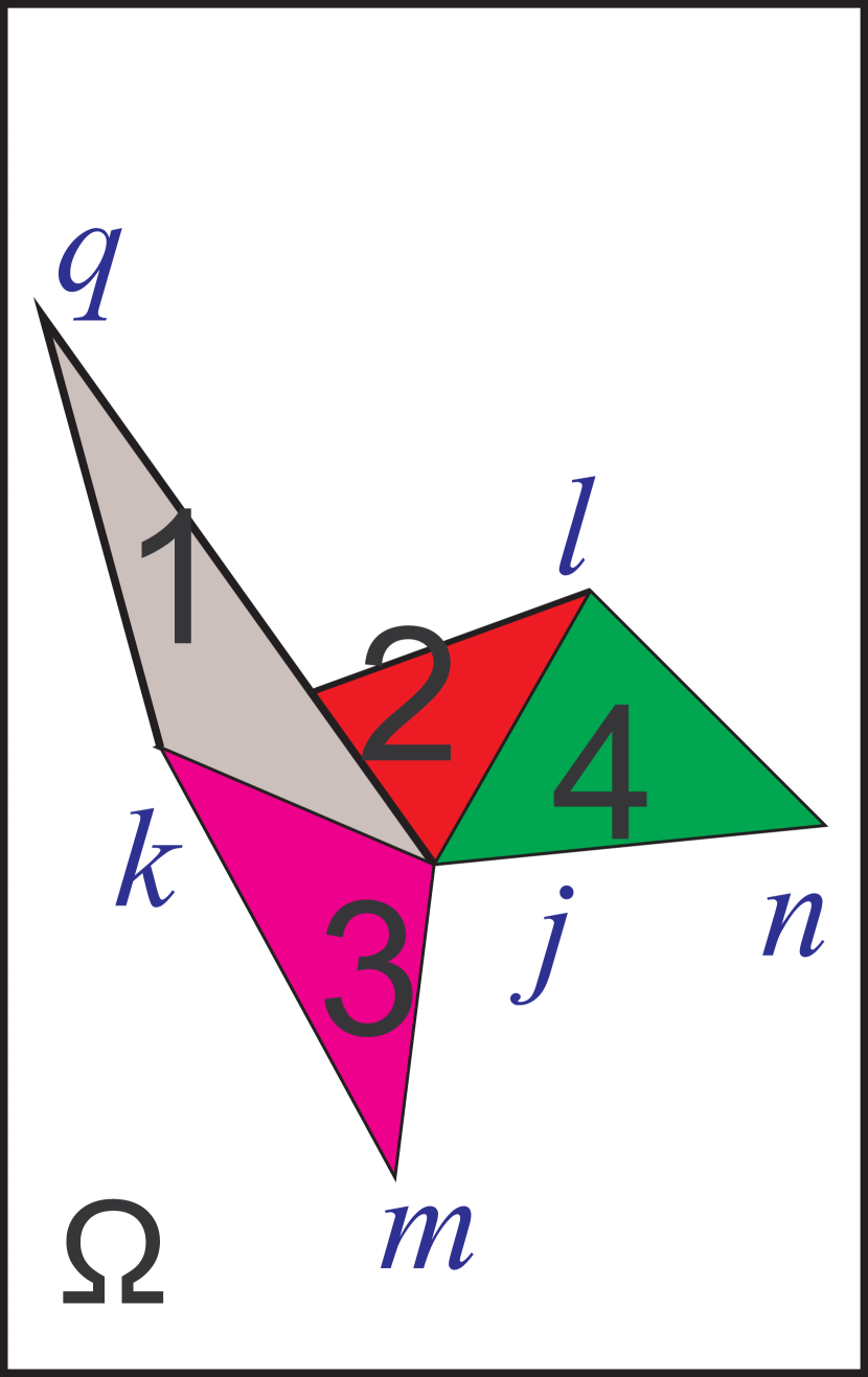
(a)

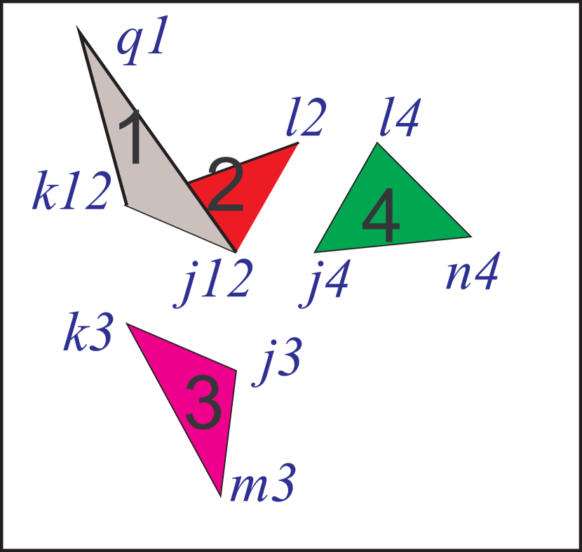
(b)

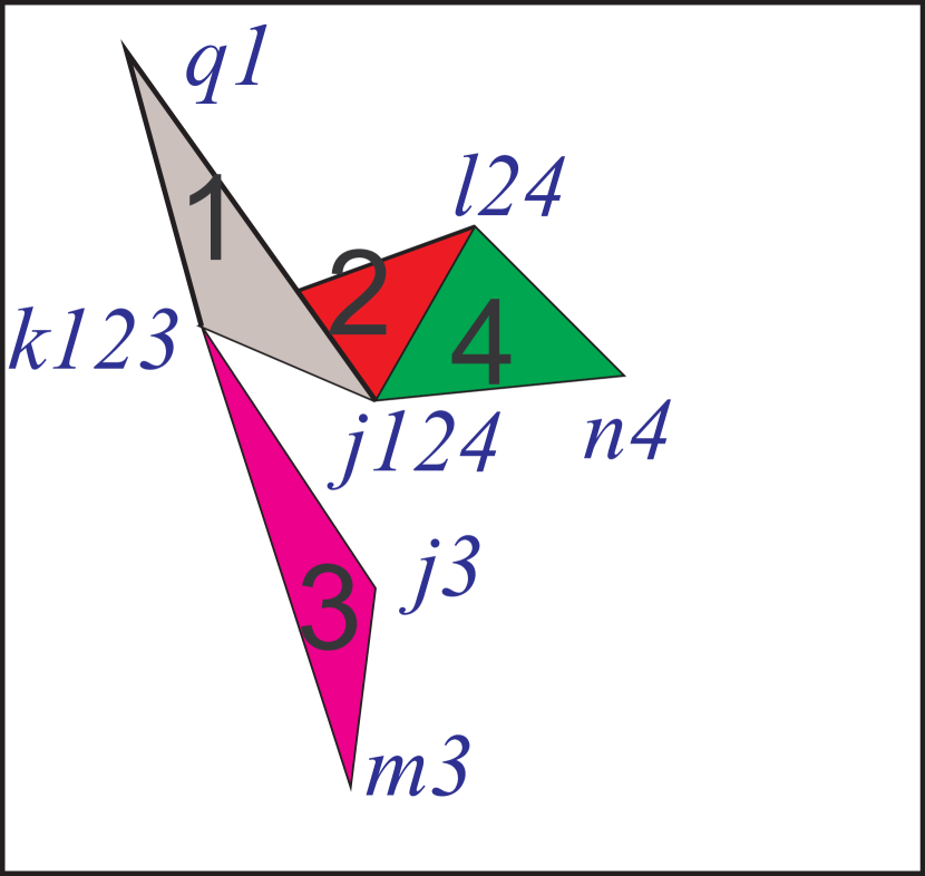
(c)

Figure C.1: Example application of Prolog primitives

In the next section we will present some code for the verification of the non-pseudomanifoldness of the complex of Example 7.4.2.

C.3 An initial quasi manifold, non pseudomanifold, 3-complex

In this section we present the Prolog program we have used to verify that the complex $\Omega$ of Example 7.4.2 could be generated by a pseudomanifold sets of instructions (see 7.2.5). First we present the instruction to build the complex $\Omega$ and verify that it is not a pseudomanifold. Next we will generate $\Omega^{\top}$, the totally decomposed version of $\Omega$, and show a set of pseudomanifold gluing instructions that turns $\Omega^{\top}$ into an isomorphic copy of $\Omega$.

It is useful to have a look to the complex of Example 7.4.2, so we reported it in Figure C.2.

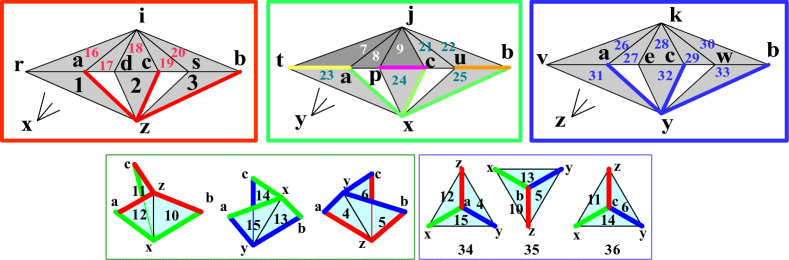
Figure C.2: A non-pseudomanifold $3$-complex generated by a non-closed pseudomanifold set of $2$-instructions

The complex $\Omega$ is the same of Figure 7.4. We kept the same numbering for top simplices (i.e. tetrahedra). Note that we used indexes 4, 5, 6, 10, 11, 12, 13, 14 and 15 to number 2-faces in the context of discussion of Example 7.4.2. For this reason, here, the 27 tetrahedra of this complex receive non contiguous indexes in the range from 1 to 36. This is not a problem due to the Prolog flexibility. Similarly vertexes are coded by non contiguous single character atoms keeping the assignments already made in the discussion of Example 7.4.2.

Looking at this figure and consulting Example 7.4.2 one can see that we are asked to build the cone from $x$ to the triangles in the red frame (see 3.2.2 for te definiton of cone). This task is done by this fragment of Prolog code:

⬇

buildRedFrame:-

addSimplex(1,[x,r,z,a]),

addSimplex(2,[x,d,z,c]),

addSimplex(3,[x,s,z,b]),

addSimplex(16,[x,r,a,i]),

addSimplex(17,[x,i,a,d]),

addSimplex(18,[x,i,c,d]),

addSimplex(19,[x,i,c,s]),

addSimplex(20,[x,i,s,b]).

Similar fragments of codes takes care to build the partial assembly of the complex $\Omega$ depicted as the cones in the green and blue frames of Figure C.2. The needed calls to addSimplex are easy to find using the numbering of Figure C.2 and they are not detailed here. The interested reader can find them in the source code available for download from GitHub [95]. So to build all the complex, first we have to complete the operations for all the cones, from x, y and z. The scheme for these cones is detailed in the three colored frames on top of Figure C.2. Then we have to add the three tetrahedra 34,35 and 36 using the numbering on the right bottom of Figure C.2. The fragment of Prolog code for all this is the following:

⬇

buildComplex:-

buildFrame,

% add the three central simplices

addSimplex(34,[x,y,z,a]),

addSimplex(35,[x,y,z,b]),

addSimplex(36,[x,y,z,c]).

% Builds the complex of the example without 3 central simplices.

buildFrame:-buildRedFrame,buildGreenFrame,buildBlueFrame.

non-pseudo-complex.pl

Now that the complex is loaded in memory, storing its TV relation, we can check if it is manifold or not. Actually, we already know that triangle xyz is common to tetrahedra 34,35,36 so it is interesting to ask Prolog to execute this fragment of code:

⬇

test1:-

resetComplex,

buildComplex,

listNonPseudoManifolds,

and the output is:

⬇

true.

that confirms our intuition. Actually, even within this trivial framework, the benefits of using Prolog is evident. We cannot say that the discussion of Example 7.4.2 is a proof of the claims we stated there. This program checks all possible triangles for non-pseudomanifoldness and returns a more reliable answer.

The next step is to show that we have an assembly to build this complex $\Omega$ from its totally exploded version $\Omega^{\top}$ using only manifold glue i.e. pseudomanifold gluing instructions (see 7.2.5).

Again we split the description of this set of gluing instructions in three subsets needed to build the cones in red, green and blue frames of Figure C.2. It is easy to see that to build the complex in the red frame from the totally exploded version $\Omega^{\top}$ we need this fragment of Prolog code:

⬇

stitchTheRedFrame:-

doPseudoManifoldGluingInstruction(1,16),

doPseudoManifoldGluingInstruction(16,17),

doPseudoManifoldGluingInstruction(17,18),

doPseudoManifoldGluingInstruction(18,2),

doPseudoManifoldGluingInstruction(18,19),

doPseudoManifoldGluingInstruction(19,20),

doPseudoManifoldGluingInstruction(20,3).

Using doPseudoManifoldGluingInstruction we are sure that, if construction do not fail, we are using gluing instructions that are pseudomanifold gluing instructions. Again, the code for the green and blue frames is similar and it is not shown here. So, in the end, we will stitch together the three cones and then stitch simplices 34,35 and 36 with the rest of the complex. This fragment of code will do the job:

⬇

stitchTheComplex:-

stitchTheRedFrame,

doPseudoManifoldGluingInstruction(1,34),

doPseudoManifoldGluingInstruction(23,34),

stitchTheGreenFrame,

doPseudoManifoldGluingInstruction(31,34),

stitchTheBlueFrame,

doPseudoManifoldGluingInstruction(3,35),

doPseudoManifoldGluingInstruction(25,35),

doPseudoManifoldGluingInstruction(33,35),

doPseudoManifoldGluingInstruction(2,36),

doPseudoManifoldGluingInstruction(24,36),

doPseudoManifoldGluingInstruction(32,36).

We note that we do not use gluing instructions that stitch two of the three tetrahedra 34,35 and 36. It will be the form of the surrounding complex that will constrain the three tetrahedra to share triangle xyz, that’s where the trick is! At least this is what intuition suggest. The gluing instructions in the code above are arranged to show that the complex is a shelllable complex i.e. during the construction of the complex $\Omega$ the gluing instructions takes care to grow a 2-connected tetrahedralization adding one new tetrahedra at every step. The new tetrahedron is introduced stitching one or more triangles between the newly added tetrahedron and the growing 3-complex. Obviously the complex $\Omega$ cannot be embedded into a three dimensional space so a formal proof of the above claims is quite appropriate.

We have a couple of tools for this. One is to use splitVertex to see if, for each vertex $v$, all vertex copies (see 5.5.1) $v_{\theta}$ created in $\Omega^{\top}$ (see 5.3.1) are collapsed into a single vertex. The predicate splitVertex(V) is the appropriate tool since it succeeds if V is a splittig vertex (see remarks after Property 5.5.1). If no splitting vertex is found this means that the gluing instructions collapses all the vertex copies $v_{\theta}$ in $\Omega^{\top}$ into a single vertex (isomorphic to) $v$. A second option is to use brute force and check that, having applied all gluing instructions, the TV and VT relations models two isomorphic simplicial complexes. The predicate vtIsoTv can do this for us. We prepared a fragment of code to stitch all together and perform the two tests.

⬇

resetDecomposition,

buildTotallyExploded,

stitchTheComplex,

not(splitVertex(_)),

vtIsoTv.

Running this we do not get any output but true. This confirms that there are no splitting vertices and that the two complexes are isomorphic.

Please note that the success of vtIsoTv is equivalent to the success of not(splitVertex(V)) because this package do not models stitching in general. Only gluing instructions that can form a decomposition of $\Omega$ from $\Omega^{\top}$ are supported. If we ask to do some gluing instruction that is not in the lattice of decompositions the relative call to doGluingInstruction fails. Therefore, what is modeled in the TV is always a complex in the lattice of decompositions (see 5.4) between $\Omega^{\top}$ and $\Omega$. The package presented here needs to be properly extended if one needs a tool for modeling simplicial complexes.

On the other hand, this limitation helps us a lot. Indeed it is not know if checking isomorphism for graphs is polynomial or even NP. Still, our trivial algorithm behind vtIsoTv checks isomorphism of the current decomposition w.r.t. the complex modeled by the TV in linear time w.r.t. the number of vertices.

Finally we can use this package to understand how this example works. To this aim we stitch all the tetrahedra but 34,35,36 and then dump splitting vertices and non pseudomanifold triangles (if any). The fragment of code for this is the following:

⬇

resetComplex,

buildComplex,

resetDecomposition,

buildTotallyExploded,

stitchTheFrame, % just build the three cones.

dumpSplitVertex,

listNonPseudoManifolds,

non-pseudo-complex.pl

where stitchTheFrame is:

⬇

stitchTheFrame:-

stitchTheRedFrame,stitchTheGreenFrame,stitchTheBlueFrame.

The output from dumpSplitVertex is quite lengthy because the complex without 34,35,36 is quite open. To give an idea of the situation we report in Figure C.3 the portion of the output that is relevant for vertex x. Arrows in figure link vertex copies of x to their location in the (not completely closed) cones.

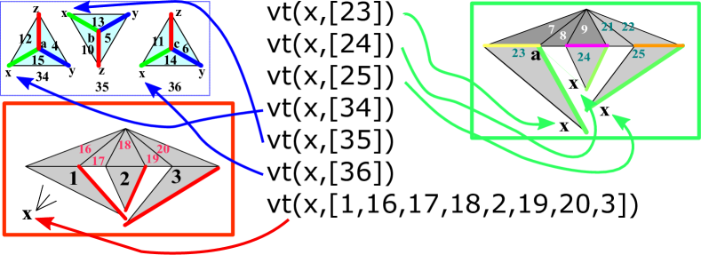
Figure C.3: the splitting vertices resulting from an incomplete stitching

On the other hand the call to listNonPseudomanifolds confirms that there are no non-pseudomanifold triangles. So we can expect to have three distinct 2-connected components, each bounded by a separate manifold surface. These hypothesis can be checked by the following code fragment:

⬇

dm1connectedComponents(C), % complex has 6 2-connected components

% Three are isolated tetrahedra.

print_term(C,[]),

boundary(Bnd), % it has a boundary surface that has 3 1-connected

% components each of 16 triangles plus three tetrahedra.

resetComplex,

addComplex(bnd,Bnd),

% now the TV holds the boundary

dm1connectedComponents(CBnd), % boundary is made up of 6 surfaces

print_term(CBnd,[]),

listNonPseudoManifolds. % no pseudomanifolds in the boundary

non-pseudo-complex.pl

output from the call to print_term(C,[]) confirms that the complex is made up of three connected components plus the three tetrahedra 34,35 and 36.

⬇

]

The first three components are the three isolated tetrahedra. The fourth component is the cone from x to the complex in the red frame in Figure C.3. The fifth component is the cone from y to the complex in the green frame. The sixth cone is not shown in Figure C.3a and is in the last line of output. The remaining (omitted) output confirms that the boundary of this complex is made up of six 1-connected surfaces without any non pseudomanifold edge. The remaining sections present the API of this package.

C.4 iqm.pl: iqm library for Initial Quasi Manifolds

Franco Morando

GPL

This program takes a simplicial complex defined via a TV relation and handles its totally decomposed version giving the possibility to stitch together top simplexes either using vertex equations or simplex gluing instructions. The totally decomposed complex is represented via VT relation

tv(?T:atom, ?V:list) [nondet]

is a dynamic predicate used to encode the TV for complex to be decomposed. If vt(foo,[a,b,c]) is stored then triangle foo with vertices a,b and c exist. User are advised to use carefully this predicate possibly ignoring it.

T & an atom that is the index of some top d-simplex.
V a set of atoms that are indexes of vertices.

vt(?V:atom, ?T:list) [nondet]

is a dynamic predicate used to encode the VT for a decomposition of the complex stored in the TV. If tv(a,[foo,bar]) is stored then top simplexes foo and bar share vertex a. To be consistent with the rest of the package no two entries like tv(a,[foo,bar]) and tv(a,[some,thing]) must exist. User are advised to use carefully this predicate possibly ignoring it.

V & an atom that is the index of some vertex.
T a set of atoms that are indexes of top simplexes.

resetComplex [det]

deletes the TV relation, complex is erased.

vtToTv(-Res:list) [det]

This procedure extracts in Res a TV from the VT representation of the complex obtained by stitching the totally decomposed complex. Indeed the stitched complex is recorded in this package in a VT using asserts to vt(V,L). This procedure leaves dynamic predicates tv/2 and vt/2 unchanged.

Res & a list of terms of the form vt($<$some vertex$>$,[s1,…,s1]) representing a VT relation.

vtIsoTv [det]

succeeds if tv and vt are isomorphic. We assume that VT is created by a call to buildTotallyExploded and several calls to doPseudoManifoldGluingInstruction or to doGluingInstruction. We recall that the effect of these two calls is the same but doPseudoManifoldGluingInstruction checks that stitching simplex is a pseudomanifold one. If not it fails.

addSimplex(+Gamma:atom, +SetGamma:list) [det]

adds a simplex to this complex Top simplexes are encoded by atoms (could be integers)

Gamma & an atom that is used as an index for the top simplex to be added.
SetGamma a set of atoms used to encode vertices for this top simplex.

addComplex(+U:atom, +SimplexList:list) [det]

adds a complex made up of a list of simplexes, e.g. [[a,b,c],[b,c,d]] for the rectangle abdc. Simplex indexes are atoms U1, U2 etc. that are created randomly using U as prefix.

U & an atom that is used as a prefix for top simplex indexes.
SimplexList a set of sets of vertices. Vertices must be encoded by atoms. e.g. [[a,b,c],[b,c,d]].

eulerX(+X:int) [det]

returns the Euler characteristics of the closed 2-complex in TV. Works only if in TV is stored a closed 2-complex. Otherwise results are meaningless.

X & the Euler characteristics of surface.

link(+V:atom, -S:list) [det]

returns the set of all maximal simplices in TV in the link of V.

V & a vertex
S a set of lists each being a maximal simplex.

star(+V:atom, -S:list) [det]

returns the set of all top simplices in TV in the star of V.

V & a vertex
S a set of atoms each being a top simplex index.

skeleton(-S:list, +D:int) [det]

returns the set of all D simplices in TV.

S & a set of sets each being a simplex.
D dimension of the simplexes to be returned D=0 for points

incident(?Theta:atom, +S:list) [nondet]

succeeds iff Theta is incident to simplex S.

Theta & an atom that is the index of some top simplex.
S a set of vertices.

orderOf(+S:list, -N:int) [det]

counts in N the number of top simplexes that are incident to the simplex given by the set of vertices in S.

S & a set of vertices.
N a positive integer that gives the number of top simplexes that are incident to S.

adjacent(?Theta1:atom, ?Theta2:atom, ?SetTheta:list) [nondet]

succeeds iff Theta1 and Theta2 are adjacent via the set of vertexes in SetTheta. If Theta1 is equal to Theta2 it fails. To succeed Theta1 and Theta2 must be two top d-simplexes and they must share the d-1 face in SetTheta.

Theta1 & an atom that is the index of some top simplex.
Theta2 an atom not equal to Theta1 that is the index of some top simplex.
SetTheta a set of vertices.

adjacent(?Theta:atom, ?Theta2:atom) [nondet]

succeeds iff Theta1 and Theta2 are adjacent. If Theta1 is equal to Theta2 it fails. Theta1 and Theta2 must be two d-simplexes and they must share a d-1 face.

Theta1 & an atom that is the index of some top simplex.
Theta2 an atom not equal to Theta1 that is the index of some top simplex.

dm1connectedComponents(-C:list) [det]

always succeeds and returns a set of sets. Each set contains atoms that are indexes of top simplices. Top simplicies in this set are uniformly dimensional. All top d-simplices in such sets are d-1 connected.

C & a set of sets of top simplexes.

nonPseudoManifold(?Theta1:atom) [nondet]

succeed if Theta1 is a top d-simplex d-1-adjacent to three or more top d simplexes.

Theta1 & an atom that is the index of some top simplex.

nonPseudoManifold(?Theta1:atom, ?SetTheta:list) [nondet]

succeeds iff the top d-simplex Theta1 is d-1 adjacent via the set of vertexes in SetTheta to three or more top d-simplexes.

Theta1 & an atom that is the index of some top d-simplex.
SetTheta a set of d-1 vertices.

nonPseudoManifoldPair(?Theta1:atom, ?Theta2:atom) [nondet]

succeed if two top d-simplexes Theta1 and Theta2 meet at a non-manifold d-1-face.

Theta1 & an atom that is the index of some top simplex.
Theta2 an atom not equal to Theta1 that is the index of some top simplex.

printSimplex(+S:atom) [det]

is a printing utility that prints the TV relation for the top simplex S.

S & an atom that is the index of some top simplex.

listNonPseudoManifolds [det]

is a listing utility that lists the set of vertices for all top d-simplexes involved in a non-manifold d-1-adjacency for some d. The utility lists also all d-1 simplexes involved in a non-manifold adjacency of top d-simplexes for some d.

listAdjacents [det]

is a listing utility that lists the set of triples [Theta1,Theta2,SetTheta] for all top d-simplexes Theta1,Theta2 involved in a d-1-adjacency via the set of vertices in SetTheta for some d.

boundaryface(+F:list) [det]

succeeds if F is d-1 face of a top d-simplex and F is on the boundary.

F & a set of d-1 vertices.

boundary(-Bnd:list) [det]

returns the list of boundary simplexes.

Bnd & a set of sets of vertices.

dumpTv [det]

lists dynamic predicate tv(T,[v1,…]) that encodes the TV for the original complex.

resetDecomposition [det]

resets the stored decomposition by deleting the VT.

buildTotallyExploded [det]

The complex given by the TV relation is turned into a totally exploded version where all top simplexes are distinct components and vertex v is split into n-copies being n the number of top simplices incident to v in the TV complex. The result is the creation of a VT relation storing vt(foo,[bar]) one for every vertex foo and for every top simplex bar. Vertices of the form vt(foo,[bar]) are called ”vertex copies” of the ”splitting vertex” foo. As stitcing operation takes place relations like vt(foo,[bar]) and vt(foo,[biz]) might disappear and will be substituted by vt(foo,[bar,biz]).

doVertexEquation(+Theta1:atom, +Theta2:atom, +V:atom) [det]

Vertexes $v_{\sigma_{1}}$ and $v_{\sigma_{2}}$ with $\theta_{1}\in\sigma_{1}$ and $\theta_{2}\in\sigma_{2}$ are identified. Note that the resulting complex, modeled by the VT relation, is a decomposition of the complex modeled by the TV relation.

Theta1 & an atom that is the index of some top simplex.
Theta2 an atom, distinct from Theta1, that is the index of some top simplex.
V a vertex that must be a vertex of Theta1 and Theta2 in the TV relation.

doGluingInstruction(+Theta1:atom, +Theta2:atom) [det]

merges vertexes according to simplex gluing instruction Theta1 $<$ Theta2.

Theta1 & an atom that is the index of some top simplex.
Theta2 an atom, distinct from Theta1, that is the index of some top simplex.

doPseudoManifoldGluingInstruction(+Theta1:atom, +Theta2:atom) [det]

merges vertexes according to simplex gluing instruction Theta1 $<$ Theta2. Before executing checks that Theta1 and Theta2 are pseudomanifold adjacent in the TV.

Theta1 & an atom that is the index of some top simplex.
Theta2 an atom, distinct from Theta1, that is the index of some top simplex.

dumpDecomp [det]

dumps each simplex for the current decomposition. The dump lists each vertex with the corresponding VT record.

splitVertex(?V:atom) [nondet]

is a topological check on the decomposition that succeeds if the vertex V has more than one vertex copy.

dumpSplitVertex [det]

dumps the VT for all splitting vertexes.

C.5 utilities.pl: utilities for application

Franco Morando

GPL

write_ln(+X) [det]

Write X on a single line

X & the item to be written.

asublist(?Sub:list, +L:list, +N:int) [nondet]

upon backtrack returns all ordered sublist of L of length N.

Sub & sublist returned.
L the complete list.
N length of the list to be returned.

disjoint(+C1:list, +C2:list) [det]

succeeds if C1 and C2 are disjoint.

C1 & and C2 two lists to be considered as sets

closurePartition(:Rel, +L:list, -Partition:list) [det]

returns the partition of L given by the quotient L/Rel*. The binary relation Rel must be symmetric and Rel* is the transitive closure of Rel.

Rel & a binary relation.
L a set of elements as a list.
Partition a list of sets one for each set in the partition. of L defined by the transitive closure of Rel.

References

- [1] Sergei I. Adyan. The unsolvability of certain algorithmic problems in the theory of groups. Trudy Moskov. Mat. Obvsvc., 6:231–298, 1957.
- [2] M. K. Agoston. Algabraic Topology: a First Course. In Pure and Applied Mathematics. Dekker, M., New York, 1976.
- [3] A.V. Aho, J.E. Hopcroft, and J.D. Ullman. Data Structures and Algorithms, Addison-Wesley. Springer Publishing Company, 1983.
- [4] Selman Akbulut and John D. McCarthy. Casson’s Invariant for Oriented Homology 3-Spheres: An Exposition. Mathematical Notes 36. Princeton University Press, Princeton, 1990.
- [5] James W. Alexander. The Combinatorial Theory of Complexes. The Annals of Mathematics, 31(2):292, 2006. doi:10.2307/1968099.
- [6] Algorithmic Solutions Software GmbH. Library of Efficient Data types and Algorithms (LEDA). In Michael S Paterson, editor, Automata, Languages and Programming, 17th International Colloquium, volume 443 of Lecture Notes in Computer Science, pages 1–5, Warwick University, England, 2012. Springer-Verlag. URL: http://www.algorithmic-solutions.com/leda/index.htm.
- [7] C. B. Allendoerfer and Frank W. Warner. Foundations of Differentiable Manifolds and Lie Groups., volume 79. Foreman and Co., Glenview, Illinois, 2006. arXiv:arXiv:1011.1669v3, doi:10.2307/2316291.
- [8] Andrew W. Appel and Guy J. Jacobson. The world’s fastest Scrabble program. In Communications of the ACM, volume 31, pages 572–578, New Orleans, Louisiana, 2002. URL: http://dl.acm.org/citation.cfm?id=314321, doi:10.1145/42411.42420.
- [9] C.R. Aragon, R. Seidel. Randomized Search Trees. In Algorithmica, volume 16, pages 464–497, 2002. doi:10.1007/s004539900061.
- [10] The U. S. Army Research Laboratory (ARL). BRL-CAD.
- [11] Gerd K. Bauer and Karl Artur Kovar. Direct HPTLC-FTIR on-line coupling: Interaction of acids and bases with the binder in precoated HPTLC plates. Journal of Planar Chromatography - Modern TLC, 11(1):30–33, 1998. doi:10.1137/0221025.
- [12] Bruce G. Baumgart. Winged edge polyhedron representation. Technical Report CS-TR-72-320, Stanford University, Department of Computer Science, oct 1972.
- [13] Walter Benjamin and Gérard Raulet. Uber den Begriff der Geschichte. Acta Univ. Szeged 2, 2:101–121, 2010.
- [14] F. Bernardini, V. Ferrucci, A. Paoluzzi, and V. Pascucci. Product operator on cell complexes. In ACM Symposium on Solid Modeling Foundations and CAD/CAM Applications, Montreal, Canada, May 19-21, 1993, pages 43–52, 2004. URL: https://doi.org/10.1145/164360.164378, doi:10.1145/164360.164378.
- [15] Fausto Bernardini and Holly Rushmeier. The 3D model acquisition pipeline. In Computer Graphics Forum, volume 21, pages 149–172. Eurographics Association, 2002. URL: http://doi.wiley.com/10.1111/1467-8659.00574, doi:10.1111/1467-8659.00574.
- [16] Y. Bertrand, J. F. Dufourd, J. Françon, and P. Lienhardt. Algebraic specification and development in geometric modeling. In Proc. TAPSOFT ’93, Orsay, France, pages 75–89, 2012. doi:10.1007/3-540-56610-4_57.
- [17] Louis J. Billera. Face Numbers of Polytopes and Complexes. In J. E. Goodman and J. O’Rourke, editors, Handbook of Discrete and Computational Geometry, number i. CRC Press, 1997.
- [18] Anders Björner and Frank H. Lutz. Simplicial manifolds, bistellar flips and a 16-vertex triangulation of the poincaré homology 3-sphere. Experimental Mathematics, 9(2):275–289, 2000. doi:10.1080/10586458.2000.10504652.
- [19] Anders Björner, Michel Las Vergnas, Bernd Sturmfels, Neil White, and Günter M. Ziegler. Oriented Matroids. In J. E. Goodman and J. O’Rourke, editors, Handbook of Discrete and Computational Geometry. CRC Press, 1993.
- [20] Anders Björner, Michel Las Vergnas, Bernd Sturmfels, Neil White, and Günter M. Ziegler. Oriented Matroids. Cambridge U. Press, Encyclopedia of Mathematics, Cambridge UK 1993, 1993.
- [21] W. M. Boothby. An Introduction to Differentiable Manifolds and Riemannian Geometry. Academic Press, 1975.
- [22] Erik Brisson. Representing geometric structures in d dimensions: topology and order. SCG 89 Proceedings of the fifth annual symposium on Computational geometry, 9(1):218–227, 1989. URL: http://www.springerlink.com/index/10.1007/BF02189330, doi:10.1145/73833.73858.
- [23] E. Bruzzone and L. De Floriani. Two Data Structures for Constructing Tetrahedralizations. The Visual Computer, 6(5):266–283, nov 1990.
- [24] E. Bruzzone, L. De Floriani, and E. Puppo. Manipulating 3D triangulations. In 3rd International Conf. FODO 1989, pages 339–353. Springer-Verlag, 1989.
- [25] J. Bryant. Piecewise Linear Topology. W. A. Benjamin, Inc., New York, 2007. doi:10.1016/b978-044482432-5/50006-8.
- [26] J. W. Cannon. Shrinking Cell-Like Decompositions of Manifolds. Codimension Three. The Annals of Mathematics, 110(1):83, 2006. doi:10.2307/1971245.
- [27] W. Charlesworth and D. C. Anderson. Applications on non-manifold topology. In Proceedings Computers in Engineering Conference and Engineering Database Symposium, pages 103–112. ASME, 1995.
- [28] Bernard Chazelle. Convex Partitions of Polyhedra: A Lower Bound and Worst-Case Optimal Algorithm. SIAM Journal on Computing, 13(3):488–507, 2005. doi:10.1137/0213031.
- [29] Harry A. Clampett. Randomized binary searching with tree structures. Communications of the ACM, 7(3):163–165, mar 2002. doi:10.1145/363958.363987.
- [30] George E. Collins. Quantifier Elimination for Real Closed Fields by Cylindrical Algebraic Decomposition. In ACM SIGSAM Bulletin, volume 10 of Lecture Notes in Computer Science, pages 10–12, Berlin, 2007. Springer-Verlag. doi:10.1145/1093390.1093393.
- [31] J. L. B. Cooper and Garrett Birkhoff. Lattice Theory, volume 34 of American Mathematical Societ Colloquium Publications. American Mathematical Society, New York, NY, third edit edition, 2007. doi:10.2307/3611622.
- [32] Thomas H. Cormen, Charles E. Leiserson, and Ronald L. Rivest. Introduction to Algorithms, Second Edition. 2001. arXiv:2010(ret.29.4.2010), doi:10.2307/2583667.
- [33] L. De Floriani. Compter Graphics (Course Notes). Technical report, Dept. of Computer Science, University of Genova, Genova, 1999.
- [34] L. De Floriani, P. Magillo, E. Puppo, and D. Sobrero. A Multi-Resolution Topological Representation for Non-Manifold Meshes. In Proceedings 7th ACM Symposium on Solid Modeling and Applications (SM02) Saarbrucken, Germany, June 17-21, 2002.
- [35] Leila De Floriani, Paola Magillo, Franco Morando, and Enrico Puppo. Non-manifold Multi-tessellation: From Meshes to Iconic Representations of Objects. In C Arcelli, L P Cordella, and G Sanniti di Baja, editors, Proceedings of the 4th International Workshop on Visual Form (IWVF4), volume 2059 of Springer-Verlag (LNCS), pages 654–664, Berlin, 2007. Springer-Verlag. doi:10.1007/3-540-45129-3_60.
- [36] Leila De Floriani, Mostefa Mohammed Mesmoudi, Franco Morando, and Enrico Puppo. Non-manifold Decomposition in Arbitrary Dimensions. In A Vialard A. Braquelaire J.-O. Lachaud, editor, Discrete Geometry for Computer Imagery (DGCI), Bordeaux, volume 2301, pages 69–80. Elsevier Science, apr 2007. URL: http://link.springer.com/10.1007/3-540-45986-3_6, doi:10.1007/3-540-45986-3_6.
- [37] H. Desaulniers and N. F. Stewart. An extension of manifold boundary representations to the r-sets. ACM Transactions on Graphics, 11(1):40–60, 2002. doi:10.1145/102377.111777.
- [38] Tamal K. Dey, Herbert Edelsbrunner, Sumanta Guha, and Dmitry V. Nekhayev. Topology Preserving Edge Contraction. Publications de l’Institut Mathématique, 66(80):23–45, 1999. URL: http://citeseerx.ist.psu.edu/viewdoc/summary?doi=10.1.1.40.7253.
- [39] Fredkin Edward. Trie memory. Commun. ACM, 3(9):490–499, sep 1960. doi:http://doi.acm.org/10.1145/367390.367400.
- [40] R. D. Edwards. The double suspension of a certain homology 3-sphere is . Notices AMS, 22:A–334, 1975.
- [41] H. G. Eggleston. Convex Polytopes, volume s1-44. Interscience Publishers John Wiley and Sons, Inc., New York, 2007. doi:10.1112/jlms/s1-44.1.663a.
- [42] J. El-Sana and Varshney A. Generalized View-Dependent Simplification. Computer Graphics Forum (Eurographics’99 Proceedings), 18(3):83–94, 1999.
- [43] Jihad El-Sana and Amitabh Varshney. Topology simplification for polygonal virtual environments. IEEE Transactions on Visualization and Computer Graphics, 4(2):133–144, 1998. doi:10.1109/2945.694955.
- [44] Hervé Elter and Pascal Lienhardt. Different Combinatorial Models based on the Map Concept for the Representation of Subsets of Cellular Complexes. In Modeling in Computer Graphics, pages 193–212, 2011. doi:10.1007/978-3-642-78114-8_12.
- [45] R. Engelking and K. Sielucki. Topology: A geometric approach. Heldermann Verlag-Berlin, 1992.
- [46] Bianca Falcidieno and Ornella Ratto. Two-manifold cell-decomposition of r-sets. In A Kilgour and L Kjelldahl, editors, Computer Graphics Forum (EUROGRAPHICS ’92 Proceedings), volume 11, pages 391–404, sep 1992.
- [47] Vincenzo Ferruci and Alberto Paoluzzi. Extrusion and boundary evaluation for multidimensional polyhedra. Computer-Aided Design, 23(1):40–50, 1991. doi:10.1016/0010-4485(91)90080-G.
- [48] M. H. Freedman and F. Luo. Selected Applications of Geometry to Low-dimensional Topology. University Lecture Series, 1, 1989.
- [49] M. H. Freedman and F. Quinn. Topology of -manifolds. Princeton University Press, 1990.
- [50] Jean Gallier. Basic Properties of Convex Sets. In J. E. Goodman and J. O’Rourke, editors, Handbook of Discrete and Computational Geometry, pages 65–83. CRC Press, 2011. doi:10.1007/978-1-4419-9961-0_3.
- [51] M. Garland and P.S. Heckbert. Simplifying surfaces with color and texture using quadric error metrics. In Proceedings IEEE Visualization’98, pages 263–269,, Research Triangle Park, NC, 2002. doi:10.1109/visual.1998.745312.
- [52] Leslie C. Glaser. Geometric combinatorial topology. Van Nostrand Reinhold, New York, 1972.
- [53] Jacob E. Goodman and Herbert Edelsbrunner. Algorithms in Combinatorial Geometry. In Brauer, W., Rozenberg, G., and Salomaa, A., editors, The American Mathematical Monthly, volume 96, page 457. Springer-Verlag, 2006. doi:10.2307/2325168.
- [54] H. B. Griffiths. Surfaces. Cambridge University Press, 1976.
- [55] André Guéziec, Frank Bossen, Gabriel Taubin, and Claudio Silva. Efficient compression of non-manifold polygonal meshes. In Computational Geometry: Theory and Applications, volume 14, pages 137–166. IEEE Comp. Soc. Press, 1999. doi:10.1016/S0925-7721(99)00027-9.
- [56] Andre Gueziec, Gabriel Taubin, Francis Lazarus, and William Horn. Converting sets of polygons to manifold surfaces by cutting and stitching. In Scott Grisson, Janet McAndless, Omar Ahmad, Christopher Stapleton, Adele Newton, Celia Pearce, Ryan Ulyate, and Rick Parent, editors, Conference abstracts and applications: SIGGRAPH 98, July 14–21, 1998, Orlando, FL, Computer Graphics, page 245, New York, NY 10036, USA, 2005. ACM Press. URL: http://www.acm.org:80/pubs/citations/proceedings/graph/280953/p245-gueziec/, doi:10.1145/280953.281628.
- [57] L. Guibas and J. Stolfi. Primitives for the Manipulation of Subdivisions. Algorithmica, 5(4):3–32, 1989.
- [58] Leonidas Guibas and Jorge Stolfi. Primitives for the manipulation of general subdivisions and the computation of Voronoi. ACM Transactions on Graphics, 4(2):74–123, apr 1985. URL: http://portal.acm.org/citation.cfm?doid=282918.282923, doi:10.1145/282918.282923.
- [59] E. L. Gursoz, Y. Choi, and F. B. Prinz. Vertex-Based Representation of Non-Manifold Boundaries. In M J Wozny, J U Turner, and K Preiss, editors, Geometric Modeling for Product Engineering, pages 107–130. Elsevier Science Publishers B.V., North Holland, 1990.
- [60] Jürgen Herzog. Combinatorics and commutative algebra, volume 41 of Progress in Mathematics. Birkhaeuser, Boston/Basel/Stuttgart, 2015. doi:10.1090/ulect/042/02.
- [61] G. Higman. UNIVERSAL ALGEBRA, volume s1-41. Van Nostrand, Princeton, first edit edition, 2007. doi:10.1112/jlms/s1-41.1.760a.
- [62] Christoph M. Hoffmann, John E. Hopcroft, Michael S. Karasick, and Ibm T.J. Watson. Robust Set Operations on Polyhedral Solids. IEEE Computer Graphics and Applications, 9(6):50–59, 1989. doi:10.1109/38.41469.
- [63] K. Janich. Topology. Springer Verlag, Berlin, 1994.
- [64] F. E. A. Johnson. On the Traingulation of Stratified Sets and Singular Varieties. Transactions of the American Mathematical Society, 275(1):333, 2006. doi:10.2307/1999023.
- [65] M. Jungerman and G. Ringel. Minimal triangulations on orientable surfaces. Acta Mathematica, 145(1):121–154, 1980. doi:10.1007/BF02414187.
- [66] John L. Kelley. General Topology., volume 27. Van Nostrand, Princeton, 1962. URL: http://www.jstor.org/stable/2964144?origin=crossref, doi:10.2307/2964144.
- [67] Lutz Kettner. Using generic programming for designing a data structure for polyhedral surfaces. Computational Geometry: Theory and Applications, 13(1):65–90, may 1999. URL: http://visinfo.zib.de/EVlib/Show?EVL-1999-40, doi:10.1016/S0925-7721(99)00007-3.
- [68] Robion C. Kirby and Laurence C. Siebenmann. Foundational Essays on Topological Manifolds, Smoothings, and Triangulations. (AM-88), volume 88 of Annals of Mathematics Studies. Princeton University Press, Princeton, 2016. doi:10.1515/9781400881505.
- [69] Reinhard Klette. Cell complexes through time. In International Symposium on Optical Science and Technology, volume 4117, pages 134–145. SPIE 4117, aug 2000. doi:10.1117/12.404813.
- [70] Donald E. Knuth. The art of computer programing. Addison-Wesley, Reading, 1997.
- [71] V. A. Kovalevsky. Finite topology as applied to image analysis. Computer Vision, Graphics, and Image Processing, 45(2):266, may 2005. doi:10.1016/0734-189x(89)90139-4.
- [72] W. Ledermann. Linear Algebra, volume 243 of Schaum’s Outline Series. McGraw-Hill, New York, NY, USA, 2013. doi:10.1038/physci243088b0.
- [73] S. H. Lee and K. Lee. Partial entity structure: a fast and compact non-manifold boundary representation based on partial topological entities. In Proceedings Sixth ACM Symposium on Solid Modeling and Applications. Ann Arbor, Michigan, jun 2001.
- [74] W. B. R. Lickorish. Simplicial moves on complexes and manifolds. Geometry and Topology Monographs: Proceedings of the Kirbyfest, 2:299–320, 2006. doi:10.2140/gtm.1999.2.299.
- [75] Julius Lieblein, Granino A. Korn, and Theresa M. Korn. Mathematical Handbook for Scientists and Engineers, volume 15. MacGraw-Hill (New York NY), 2006. doi:10.2307/2003035.
- [76] P. Lienhardt. Subdivisions of n -dimensional spaces and n -dimensional generalized maps . In Proceedings 5th ACM Symposium on Computational Geometry, Saarbrucken, Germany, pages 228–236, 2003. doi:10.1145/73833.73859.
- [77] P. Lienhardt. N-Dimensional Generalized Combinatorial Maps and Cellular Quasi-Manifolds. Technical Report 03, Universite Louis Pasteur, Strasbourg, 2004. doi:10.1142/s0218195994000173.
- [78] Pascal Lienhardt. Topological models for boundary representation: a comparison with n-dimensional generalized maps. Computer-Aided Design, 23(1):59–82, 1991. doi:10.1016/0010-4485(91)90082-8.
- [79] Pascal Lienhardt. Aspects in Topology-Based Geometric Modeling. Lecture Notes in Computer Science, 1347, 1997.
- [80] Pascal Lienhardt. n-dimensional generalized combinatorial maps and cellular quasi-manifolds. International Journal of Computational Geometry and Applications, 04(03):275–324, 2004. doi:10.1142/s0218195994000173.
- [81] Hélio Lopes and Geovan Tavares. Structural operators for modeling 3-manifolds. In SMA ’97: Proceedings of the Fourth Symposium on Solid Modeling and Applications, pages 10–18. ACM, may 2004. doi:10.1145/267734.267745.
- [82] David Luebke and Carl Erikson. View-dependent simplification of arbitrary polygonal environments. In SIGGRAPH 97 Proc., pages 199–208, aug 2005. doi:10.1145/258734.258847.
- [83] P. M. Cohn. Universal Algebra. Reidel, Dordrecht, second edition, 1981.
- [84] I. G. MacDonald. Convex Polytopes and the Upper Bound Conjecture, volume 5 of London Math. Soc. Lecture Notes Series. Cambridge Univ. Press, Cambridge UP, 2007. doi:10.1112/blms/5.1.119.
- [85] M. Mäntylä. A Note on the Modeling Space of Euler Operators. Computer Vision, Graphics and Image Processing, 26(1):45–60, 1984.
- [86] Martti Mäntylä. An Introduction to Solid Modeling, volume 8. Computer Science Press, 1988. URL: http://www.sciencedirect.com/science/article/pii/0097849384900438, doi:http://dx.doi.org/10.1016/0097-8493(84)90043-8.
- [87] Mark Allen Weiss. Livre Data Structures And Algorithm Analysis In C++. Addison_Wesley, 2006. URL: http://medcontent.metapress.com/index/A65RM03P4874243N.pdf%5Cnhttp://link.springer.com/content/pdf/10.1007/978-0-387-69008-7.pdf, doi:10.1002/1521-3773(20010316)40:6<9823::AID-ANIE9823>3.3.CO;2-C.
- [88] A. A. Markov. The insoluability of the problem of homeomorphy. In Dokl. Akad. Nauk. SSSR., volume 121, pages 218–220, 1958.
- [89] H. Masuda. Topological operators and Boolean operations for complex-based nonmanifold geometric models. Computer-Aided Design, 25(2):119–129, feb 1993. doi:10.1016/0010-4485(93)90097-8.
- [90] Sara McMains, Joseph M. Hellerstein, and Carlo H. Séquin. Out-of-core build of a topological data structure from polygon soup. Solid Modeling, pages 171–182, 2004. doi:10.1145/376957.376977.
- [91] Sara McMains and Carlo Séquin. A coherent sweep plane slicer for layered manufacturing. Proceedings of the Symposium on Solid Modeling and Applications, pages 285–295, 2004. doi:10.1145/304012.304042.
- [92] Sara Anne McMains. Geometric Algorithms and Data Representation for Solid Freeform Fabrication. Ph.D. thesis, University of California, Berkeley, CA, 2000. URL: http://www.me.berkeley.edu/$∼$mcmains/pubs/thesis.pdf.
- [93] John Milnor. Two Complexes Which are Homeomorphic But Combinatorially Distinct. The Annals of Mathematics, 74(3):575, 2006. doi:10.2307/1970299.
- [94] Edwin E. Moise. Affine Structures in 3-Manifolds: V. The Triangulation Theorem and Hauptvermutung. The Annals of Mathematics, 56(1):96, 2006. doi:10.2307/1969769.
- [95] F. Morando. IQM A Prolog package for Initial Quasi Manifold decomposition. https://github.com/francomorando/IQM, mar 2003. URL: https://github.com/francomorando/IQM.
- [96] D Mount. CMSC 420: Data Structures (Lecture Notes). Technical report, University of Maryland, College Park, MD, 1993.
- [97] D. Mount. CMSC 251: Algorithms (Lecture Notes). Technical report, University of Maryland, College Park, MD, 1998.
- [98] D. E. Muller and F. P. Preparata. Finding the intersection of two convex polyhedra. Theoretical Computer Science, 7(2):217–236, oct 1978. doi:10.1016/0304-3975(78)90051-8.
- [99] M. J. Muuss and L. A. Butler. Combinatorial Solid Geometry, Boundary Representations, and non-Manifold Geometry. In D F Rogers and R A Earnshaw, editors, State of the Art in Computer Graphics: Visualization and Modeling, pages 185–223. Springer-Verlag, Berlin, Germany, 1991.
- [100] A. Nabutovsky. Geometry of the space of triangulations of a compact manifold. Communications in Mathematical Physics, 181(2):303–330, 1996. URL: https://projecteuclid.org:443/euclid.cmp/1104287765, doi:10.1007/BF02101007.
- [101] M. H. A. Newman. A theorem in combinatorial topology. J. London Math. Soc., 6:186–192, 1931.
- [102] Isabella Novik. Upper bound theorems for homology manifolds. Israel Journal of Mathematics, 108:45–82, 1998. doi:10.1007/BF02783042.
- [103] A. Paoluzzi, F. Bernardini, C. Cattani, and V. Ferrucci. Dimension-independent modeling with simplicial complexes. ACM Transactions on Graphics, 12(1):56–102, jan 2002. doi:10.1145/169728.169719.
- [104] Christos D. Papakyriakopoulos. A new proof of the invariance of the homology groups of a complex. Bull. Soc. Math. Grèce, 22:1–154, 1943.
- [105] P. J. Plauger, Alexander A. Stepanov, Meng Lee, and David R. Musser. The C++ Standard Template Library. Prentice-Hall, Upper Saddle River, NJ 07458, USA, 2000.
- [106] Jovan Popović and Hugues Hoppe. Progressive simplicial complexes. In ACM Computer Graphics Proceedings, Annual Conference Series, (SIGGRAPH ’97), pages 217–224, 2005. URL: http://research.microsoft.com/$∼$hoppe/siggraph97psc.ps.gz, doi:10.1145/258734.258852.
- [107] R. C. Kirby and L.C. Siebenmann. on the Triangulation of Manifolds and the Hauptvermutung. Bulletin of the American Mathematical Society, 75(4):742–749, 1969.
- [108] K. Reidemeister. Topologie der Polyeder und kombinatorische Topologie der Komplexe, volume 49. Akad Verlagsgesellschaft, Geest und Portig (Leipzig), 2005. doi:10.1007/bf01707363.
- [109] A. A. G. Requicha. Representations of Rigid Solids: Theory, Methods, and Systems. ACM Computing Surveys, 12(4):437–464, 1980.
- [110] Solid Modeling Solutions (). . URL: http://www.smlib.com/.
- [111] Remi Ronfard and Jarek Rossignac. Full-range approximation of triangulated polyhedra. Computer Graphics Forum, 15(3):67–76, aug 2003. doi:10.1111/1467-8659.1530067.
- [112] J. R. Rossignac and M. A. O’Connor. SGC: A dimension-indipendent model for pointsets with internal structures and incomplete boundaries. In J U Turner M. J. Wozny and K Preiss, editors, Geometric Modeling for Product Engineering, pages 145–180. Elsevier Science Publishers B.V. (North–Holland), Amsterdam, 1990.
- [113] Jarek Rossignac and Paul Borrel. Multi-resolution 3D approximations for rendering complex scenes. In B Falcidieno and T L Kunii, editors, Modeling in Computer Graphics, pages 455–465. Springer Verlag, 2011. doi:10.1007/978-3-642-78114-8_29.
- [114] Jarek Rossignac and David Cardoze. Matchmaker: Manifold BReps for Non-Manifold R-Sets. In Willem F Bronsvoort and David C Anderson, editors, Proceedings of the Fifth Symposium on Solid Modeling and Applications (SSMA-99), pages 31–41, New York, jun 1999. ACM Press.
- [115] Gian-Carlo Rota. On the Foundations of Combinatorial Theory. In Classic Papers in Combinatorics, volume 29, pages 332–360, 2010. doi:10.1007/978-0-8176-4842-8_25.
- [116] W.J. Schroeder. A topology modifying progressive decimation algorithm. In R Yagel and H Hagen, editors, IEEE Visualization ’97 Proceedings, pages 205–212,. IEEE Press, 2002. doi:10.1109/visual.1997.663883.
- [117] Kuntal Sengupta and Kim L. Boyer. Organizing Large Structural Modelbases. IEEE Transactions on Pattern Analysis and Machine Intelligence, 17(4):321–332, apr 1995. doi:10.1109/34.385984.
- [118] Topological Spaces. Computational Topology : Basics. In J. E. Goodman and J. O’Rourke, editors, Handbook of Discrete and Computational Geometry, pages 1–8. CRC Press, 2010.
- [119] Edwin H. Spanier. Algebraic Topology. 1981. doi:10.1007/978-1-4684-9322-1.
- [120] Ram D. Sriram, Albert Wong, and Li Xing He. Gnomes: an Object-Oriented Nonmanifold Geometric Engine. Computer-Aided Design, 27(11):853–868, 1995. doi:10.1016/0010-4485(95)00022-4.
- [121] Silicon Graphics Computer Systems. Standard Template Library Programmer’s Guide. 1999.
- [122] Gabriel Taubin and Jarek Rossignac. Geometric compression through topological surgery. ACM Transactions on Graphics, 17(2):84–115, jan 2002. doi:10.1145/274363.274365.
- [123] Abigail Thompson. Thin Position and the Recognition Problem for . Mathematical Research Letters, 1(5):613–630, 2013. doi:10.4310/mrl.1994.v1.n5.a9.
- [124] A. W. Tucker. An Abstract Approach to Manifolds. The Annals of Mathematics, 34(2):191, 2006. doi:10.2307/1968201.
- [125] I A Volodin, V E Kuznetsov, and A T Fomenko. The problem of discriminating algorithmically the standard three dimensional sphere. Russian Mathematical Surveys, 29(5):71–172, 2005. doi:10.1070/rm1974v029n05abeh001296.
- [126] C.T.C. Wall. Regular stratifications. In Warwack, Lecture Notes on dynamic systems, pages 332–344. Springer-Verlag, 2006. doi:10.1007/bfb0082632.
- [127] K. Weiler. Boundary Graph Operators for Non-Manifold Geometric Modeling Topology Representations. In H. W. McLaughlin J.L. Encarnacao M.J. Wozny, editor, Geometric Modeling for CAD Applications, pages 37–66. Elsevier Science Publishers B.V. (North–Holland), Amsterdam, 1988.
- [128] K. Weiler. Vertex Neighborhood Topological Information and Data Structures in a Non-Manifold Environment. Technical report, Autodesk, apr 1996.
- [129] Kevin Weiler. Edge-Based Data Structures for Solid Modeling in Curved-Surface Environments. IEEE Computer Graphics and Applications, 5(1):21–40, 1985. doi:10.1109/MCG.1985.276271.
- [130] Kevin Weiler. Topological Structures for Geometric Modeling. Ph.D. thesis, Computer and Systems Engineering, Rennselaer Polytechnic Institute, Troy, NY, aug 1986.
- [131] Kevin Weiler. The radial edge structure: a topological representation for non-manifold geometric boundary modeling. In H W McLaughlin J.L. Encarnacao M.J. Wozny, editor, Geometric modeling for CAD applications, pages 3–36. Elsevier Science Publishers B.V. (North–Holland), Amsterdam, 1988. URL: http://scholar.google.com/scholar?hl=en&btnG=Search&q=intitle:The+radial+edge+structure:+A+topological+representation+for+non-manifold+geometric+boundary+modeling#0.
- [132] Philip M. Whitman. Free Lattices. The Annals of Mathematics, 42(1):325, 2006. doi:10.2307/1969001.
- [133] Hassler Whitney. Elementary Structure of Real Algebraic Varieties. The Annals of Mathematics, 66(3):545, nov 2006. doi:10.2307/1969908.
- [134] Jan Wielemaker. An Overview of the SWI-Prolog Programming Environment. In Fred Mesnard and Alexander Serebenik, editors, WLPE’03: Proceedings of the 13th International Workshop on Logic Programming Environments, pages 1–16, Heverlee, Belgium, 2003. Katholieke Universiteit Leuven.
- [135] P. R. Wilson. Data Transfer and Solid Modeling. In H W McLaughlin J.L. Encarnacao M.J. Wozny, editor, Geometric Modeling for CAD Applications, pages 217–254. Elsevier Science Publishers B.V. (North–Holland), Amsterdam, 1988.
- [136] Tony C. Woo. A Combinatorial Analysis of Boundary Data Structure Schemata. IEEE Computer Graphics and Applications, 5(3):19–27, mar 1985. doi:10.1109/MCG.1985.276337.
- [137] Yasushi Yamaguchi and Fumihiko Kimura. Non-manifold topology model based on coupling entities. IEEE Computer Graphics and Applications, 15(1):537, jan 2004. doi:10.1145/112515.112592.
Index
-