Optimal Number of Measurements in a Linear System with Quadratically Decreasing SNR

Abstract

We consider the design of a linear sensing system with a fixed energy budget assuming that the sampling noise is the dominant noise source. The energy constraint implies that the signal energy per measurement decreases linearly with the number of measurements. When the maximum sampling rate of the sampling circuit is chosen to match the designed sampling rate, the assumption on the noise implies that its variance increases approximately linearly with the sampling rate (number of measurements). Therefore, the overall SNR per measurement decreases quadratically in the number of measurements. Our analysis shows that, in this setting there is an optimal number of measurements. This is in contrast to the standard case, where noise variance remains unchanged with sampling rate, in which case more measurements imply better performance. Our results are based on a state evolution technique of the well-known approximate message passing algorithm. We consider both the sparse (e.g. Bernoulli-Gaussian and least-favorable distributions) and the non-sparse (e.g. Gaussian distribution) settings in both the real and complex domains. Numerical results corroborate our analysis.

I Introduction

The problem of estimating a signal from its linear measurements has been studied for many decades. From linear algebra, at least $n$ measurements are required in order to ensure the reconstruction of an $n$-dimensional signal. Otherwise, the solution is not unique. The field of compressed sensing (CS) [2, 3] has shown that when the unknown signal is sparse, assuming no further prior knowledge on the signal, the number of measurements can be reduced below the dimension of the signal leading to an underdetermined linear measurement system. Many low complexity algorithms have been proposed to solve the resulting sparse recovery problem including greedy algorithms, for example orthogonal matching pursuit (OMP) [4], subspace pursuit (SP) [5] and compressive sampling matching pursuit (CoSaMP) [6], $\ell_{1}$-norm minimisation [7], and more recently approximate message passing (AMP) [8]. CS has been widely used in under-sampling [9, 10, 8, 11], imaging and localisation [12, 13, 14], and sparse learning [15].

In this paper, we study a system design problem with focus on the sampling rate. That is, based on the typical characteristics of the acquired signals, our goal is to choose an optimal number of measurements to minimise the mean squared error (MSE) of the recovery. We assume that the signal’s dimension, sparsity level, and statistics are given. We also make two assumptions on the sampling process. First, since practical systems are power limited, the energy in the measurements for a fixed time period is fixed. This implies that the energy per measurement decreases linearly with the number of measurements (or equivalently sampling rate). Second, we assume that the sampling noise is the dominant noise source. In addition, in order to minimise hardware cost, the sampling circuit is chosen to operate at its maximum sampling rate. We model the sampling noise as additive white Gaussian noise. The noise variance of the sampling circuit follows the well known $KT/C$ rule [16, 17, 18], where $K$ is the Boltzmann’s constant, $T$ is the absolute temperature of the circuit, and $C$ is the capacitance of the sampling circuit which is inversely proportional to the maximum and optimal sampling rate based on our assumption. This implies that the noise variance increases approximately linearly with the number of measurements. In addition, although quantisation noise is not studied in this paper, it is widely observed that the effective number of bits of an analog-to-digital converter decreases when the sampling frequency increases [20]. This also results in the phenomenon that higher sampling rate implies larger noise variance. The combined effect of these two assumptions is that the SNR per measurement decreases quadratically as a function of the number of measurements.

In practical systems, other noise sources exist such as additive noise before sampling (also known as signal noise) [19, 20] and quantisation noise[21, 22]. In this paper, we focus on the effect of sampling noise, leaving analysis of the effects of other noises as possible future work.

Under a quadratically decreasing SNR system, our goal is to analyse the optimal number of measurements. Different from the standard setting where noise variance remains unchanged with sampling rate and hence more measurements typically means better recovery performance, we show that with quadratically decreasing SNR more measurements do not necessarily imply better recovery.

More specifically, we demonstrate that in the quadratically decreasing SNR scenario, there exists an optimal normalised number $\delta^{\dagger}$ of measurements to minimise the mean squared error (MSE) of the recovered signal. Here $\delta=\frac{m}{n}$, where $m$ is the number of measurements and $n$ is the dimension of the unknown signal. We explicitly study three signal models: Gaussian, Bernoulli-Gaussian and least-favorable distributions in both the real and complex domains. We obtain closed-form expressions for $\delta^{\dagger}$ in the Gaussian and least-favorable models and provide a numerical procedure to find the optimal $\delta^{\dagger}$ in other cases. We show that for the three models, $\delta^{\dagger}\leq 2$. Furthermore, when the SNR is low, $\delta^{\dagger}$ can be smaller than $1$ implying that $m<n$ in both the sparse and non-sparse models. In particular, $\delta^{\dagger}<1$ in the Gaussian model when $\sigma_{x}^{2}<2\sigma_{0}^{2}$ where $\sigma_{x}^{2}$ is the signal variance and $\sigma_{0}^{2}$ is the noise base level, defined in Section II-B. For sparse vectors we require in addition that $\epsilon=\frac{S}{n}$ is smaller than roughly $0.2$ where $S$ is the number of non-zero elements in the unknown signal.

Our analysis and results are based on the AMP algorithm and the associated state evolution. Though rigorous derivation of the state evolution of AMP requires a random Gaussian matrix, many works have demonstrated that the same results are relatively accurate for partial Fourier and Rademacher matrices [8, 23] when the sizes of these matrices are sufficiently large.

The rest of this paper is organised as follows: In Section II we introduce our problem and mathematically explain the quadratically decreasing SNR model. We also provide the relationship between $\delta^{\dagger}$ and the MSE in the Gaussian setting based on random matrix theory. In Section III, we introduce AMP and state evolution which are used for sparse recovery. The analysis of least-favorable and Bernoulli-Gaussian models is developed in Section IV for the real case and in Section V for the complex case. Bounds on the optimal number of measurements and discussion about the specific situation in which $\delta^{\dagger}<1$ are provided in Section VI, followed by conclusions.

II System Model

II-A Quadratically Decreasing SNR Model

Consider the linear system

$$\bm{y}=\bm{s}+\bm{w},$$ (1)

where $\bm{y}\in\mathbb{H}^{m}$ is the observation vector, $\bm{s}\in\mathbb{H}^{m}$ represents an unknown signal vector and $\bm{w}\in\mathbb{H}^{m}$ is additive white Gaussian noise. Here, $\mathbb{H}\in\left\{\mathbb{R},\mathbb{C}\right\}$ where $\mathbb{R}$ denotes the real domain and $\mathbb{C}$ the complex domain.

Assume the system has a fixed energy budget $E_{s}$, so that the total energy that can be allocated to $\bm{s}$ is

$$E_{s}=\sum_{i=1}^{m}\left|s_{i}\right|^{2}.$$ (2)

The corresponding average energy per signal sample is

$$P_{as} =\frac{1}{m}\sum_{i=1}^{m}\left|s_{i}\right|^{2}=\frac{1}{m}E_{s}\propto\frac{1}{m}.$$ (3)

In practice, noise is unavoidable and comes from different parts of the system. Consider the signal acquisition scheme illustrated in Fig. 1. The received analog signal first passes through a low pass or band pass filter, which filters the out of band noise. We refer to the remaining in-band noise as signal noise. The filtered signal is then sampled which produces sampling noise. After that, a quantiser is applied to convert the samples to bits which leads to quantisation errors. In [19, 20, 21], the authors discuss the signal noise and the corresponding noise folding effect. Quantisation error was studied in [22]. A combined analysis of the signal noise and quantisation errors is provided in [21] with the assumption of a fixed bit-budget on the measurements.

Figure 1: Signal acquisition system.

The sampling noise (i.e. thermal noise in the sampling circuit) is often the dominant noise source, for example in radar systems [24, pp 5.21-5.26] and magnetic resonance imaging (MRI) systems [25]. Here we focus on the impact of sampling noise by assuming that both signal noise and quantisation errors are relatively small. Based on [16, 17, 18], the variance of sampling noise is approximately given by $KT/C$ where $K$ is the Boltzmann’s constant, $T$ is the absolute temperature of the circuit and $C$ is the sampling capacitance. The speed of the sampling circuit (which can be simplified as a switched-capacitor circuit) depends on the on-resistance of the switch and the sampling capacitance $C$. A high speed sampling circuit requires a small sampling capacitor. From the system design point of view, there is a trade-off between the sampling noise (with variance $KT/C$) and the designed sampling speed. This phenomenon is discussed in Chapter 12 of [18] in detail. Here we emphasise that the sampling noise in the sampling circuit is independent of the bandwidth of the signal $\bm{s}$ and only depends on the sampling rate of the circuit.

As discussed above, the noise variance increases approximately linearly with the number of measurements. The average energy per noise sample is then

$$P_{an} \propto f_{s}\propto m$$

where $f_{s}$ is the sampling frequency. With these definitions, the SNR is proportional to

$${\rm SNR}=\frac{P_{as}}{P_{an}}\propto\frac{\frac{1}{m}}{m}=\frac{1}{m^{2}}$$

which is a quadratic decreasing model with respect to the number of measurements $m$.

We have implicitly assumed that the signal noise and the quantisation error are negligible compared to the sampling noise [24, 25]. In reality, the former two noises will create a small but nonzero noise floor with constant variance. As the variance of the noise floor depends on system specifications, we leave the detailed design considering all noise sources as a future research topic.

II-B General Linear System Model

We now extend the model in (1) to a general linear model

$$\bm{y}=\bm{A}\bm{x}+\bm{w}$$ (4)

where $\bm{A}\bm{x}\coloneqq\bm{s}$, $\bm{A}\in\mathbb{H}^{m\times n}$ denotes the measurement matrix and $\bm{x}$ represents the unknown signal vector. In order to incorporate the quadratically decreasing SNR assumption, we define $\bm{A}$ as a Gaussian random matrix with elements i.i.d. drawn from $\mathcal{N}\left(0,\frac{1}{m}\right)$ or $\mathcal{CN}\left(0,\frac{1}{m}\right)$. The elements of $\bm{x}$ are assumed to be i.i.d. drawn from a distribution $p_{x}$ with zero mean and variance independent of $m$. We assume the noise is Gaussian $\mathcal{N}\left(0,\sigma_{w}^{2}\right)$ or $\mathcal{CN}\left(0,\sigma_{w}^{2}\right)$ with

$$\sigma_{w}^{2}\coloneqq\delta\sigma_{0}^{2}$$ (5)

where $\delta\coloneqq\frac{m}{n}$ and $\sigma_{0}^{2}$ is the constant noise base level.

Let $\hat{\bm{x}}$ be an estimate of $\bm{x}$. The associated MSE is defined by

$${\rm Err} =\lim_{n\rightarrow\infty}\frac{1}{n}{\rm{\rm\mathbb{E}}}\left[\left\|\bm{x}-\hat{\bm{x}}\right\|^{2}\right].$$ (6)

Under the quadratically decreasing SNR model we want to determine the optimal number of measurements $m$ to minimise the MSE in estimating $\bm{x}$. In particular, an interesting question is whether there are cases where $m$ is smaller than $n$, which would imply an under-sampling scenario. We consider the system model (4) for both non-sparse and sparse signals.

II-C Non-Sparse Setting

To gain intuition, we start by considering a Gaussian model. Assume that $\bm{x}$ is drawn from $\mathcal{N}\left(\bm{0},\sigma_{x}^{2}\bm{I}\right)$ when $\mathbb{H}=\mathbb{R}$ (or $\mathcal{CN}\left(\bm{0},\sigma_{x}^{2}\bm{I}\right)$ when $\mathbb{H}=\mathbb{C}$) and the noise $\bm{w}$ is drawn from $\mathcal{N}\left(\bm{0},\sigma_{w}^{2}\bm{I}\right)$ when $\mathbb{H}=\mathbb{R}$ (or $\mathcal{CN}\left(\bm{0},\sigma_{w}^{2}\bm{I}\right)$ when $\mathbb{H}=\mathbb{C}$). The asymptotic MSE (6) of the MMSE estimator can then be directly calculated based on random matrix theory [26]. Denoting $c=\frac{\left(1-\delta\right)}{\delta}$, we have

$${\rm Err}=\!\frac{\delta}{2}\left[\left(\!-\!\sigma_{w}^{2}\!\!+\!c\sigma_{x}^{2}\right)\!\!+\!\!\sqrt{\!\left(\sigma_{w}^{2}\!\!+\!c\sigma_{x}^{2}\right)^{2}\!\!+\!4\sigma_{w}^{2}\sigma_{x}^{2}}\right].$$ (7)

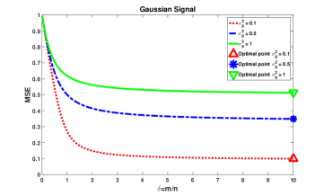
(a) Traditional Case: $\sigma_{w}^{2}=\sigma_{0}^{2}$ is constant

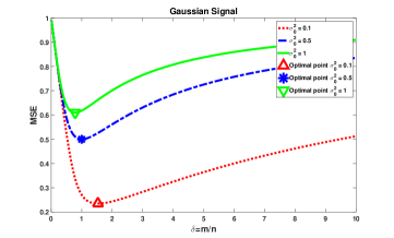
(b) Our Case: $\sigma_{w}^{2}=\delta\sigma_{0}^{2}$ varies with $\delta$

Figure 2: MSE in a non-sparse Gaussian model.

An illustration of the MSE for the case in which $\sigma_{x}^{2}=1$ and $\sigma_{w}^{2}=\sigma_{0}^{2}$ is provided in Fig. 2a. The MSE is calculated via (7) and we choose three different values for $\sigma_{0}^{2}$: $0.1$, $0.5$ and $1$. The simulation results reflect, in the traditional case, that more measurements provide better performance. When we replace the noise variance with our model (5), a trade-off between MSE and $\delta$ exists. Figure 2b shows that there is an optimal number of measurements that minimizes the MSE which is quit different from the traditional case. The optimal values of $\delta$ for the three curves ($\sigma_{0}^{2}=0.1$, $0.5$ and $1$) are smaller than $2$; when $\sigma_{0}^{2}=1$, the optimal $\delta$ is even smaller than $1$ (i.e. $m<n$). A detailed discussion regarding bounds on $\delta^{\dagger}$ and the situation in which $\delta^{\dagger}<1$ is provided in Section VI-A.

Motivated by this phenomenon, our goal is to find a similar relationship for sparse signals by taking into account the nonlinear property of the sparse decoder.

III Approximate Message Passing

In order to treat sparse signals, a sparse decoder is required for signal recovery. We choose the AMP algorithm which has low computational complexity per iteration, fast convergence speed (when it converges), and good performance guarantees (with a standard Gaussian random matrix). Exact performance of AMP can be predicted via the so called state evolution (SE) technique.

The AMP algorithm was first proposed in [8] to solve (4) in the CS scenario in which $m<n$ and $\bm{x}$ is assumed to be sparse. It iteratively applies the following equations:

$$\bm{x}^{t+1} =\! \eta\left(\bm{A}^{*}\bm{r}^{t}+\bm{x}^{t}\right),$$ (8)

$$\bm{r}^{t} =\! \bm{y}\!-\!\bm{A}\bm{x}^{t}+\frac{1}{\delta}\!\left\langle\eta^{\prime}\!\left(\bm{A}^{*}\bm{r}^{t-1}\!+\!\bm{x}^{t-1}\right)\!\right\rangle\!\bm{r}^{t-1},$$ (9)

where $\bm{x}^{t}$ denotes the $t$-th estimation of $\bm{x}$, $\eta\left(\cdot\right)$ is a component-wise estimator designed based on the statistical information on its input argument, $\bm{A}^{*}$ stands for the (conjugate) transpose of $\bm{A}$, $\eta^{\prime}$ represents the first order derivative of $\eta$, and $\left\langle\bm{v}\right\rangle:=\frac{1}{n}\sum_{i=1}^{n}v_{i}$ computes the average. The last term of (9)

$${\rm Onsager}\coloneqq\frac{1}{\delta}\left\langle\eta^{\prime}\left(\bm{A}^{*}\bm{r}^{t-1}+\bm{x}^{t-1}\right)\right\rangle\bm{r}^{t-1},$$ (10)

is called the Onsager (correction) term.

A heuristic suggestion was presented in [26, 27] to analyse the performance of AMP. The idea is to decompose the input of the function $\eta\left(\bm{\beta}^{t}\right)$ into the superposition of the original signal $\bm{x}$ and white Gaussian noise. Consider three modifications at each iteration $t$: replace 1) the matrix $\bm{A}$ with a new independent copy $\bm{A}\left(t\right)$, 2) the observation vector $\bm{y}$ with $\bm{y}^{t}=\bm{A}\left(t\right)^{*}\bm{x}+\bm{w}$, and 3) the Onsager term in (9) with $\bm{0}$. The input of $\eta\left(\bm{\beta}^{t}\right)$ can then be written as

$$\bm{\beta}^{t} \coloneqq\bm{A}\left(t\right)^{*}\bm{r}^{t}+\bm{x}^{t}=\bm{A}\left(t\right)^{*}\left(\bm{y}^{t}-\bm{A}\left(t\right)\bm{x}^{t}\right)+\bm{x}^{t}$$

$$=\bm{x}+\left(\bm{A}\left(t\right)^{*}\bm{A}\left(t\right)-\bm{I}\right)\left(\bm{x}-\bm{x}^{t}\right)+\bm{A}\left(t\right)^{*}\bm{w}$$ (11)

which is the ground truth signal $\bm{x}$ plus an equivalent noise:

$$\bm{w}_{e}^{t}\coloneqq\left(\bm{A}\left(t\right)^{*}\bm{A}\left(t\right)-\bm{I}\right)\left(\bm{x}-\bm{x}^{t}\right)+\bm{A}\left(t\right)^{*}\bm{w}.$$ (12)

Although in the AMP algorithm, we do not have independent copies $\bm{A}\left(t\right)$ as well as independent observations $\bm{y}^{t}$, due to the Onsager term, the statistical information of the equivalent noise can still be asymptomatically calculated via (12) which may be treated as approximately Gaussian and independent of $\bm{x}$. At each iteration $t$, we first update the estimated signal $\bm{x}^{t+1}=\eta\left(\bm{\beta}^{t}\right)$ by a particularly designed $\eta\left(\cdot\right)$ function (detailed information is provided in Sections IV and V) which depends on the knowledge of the signal $\bm{x}$ and the equivalent noise $\bm{w}_{e}^{t}$ (i.e. $\sigma_{e}^{t}$, the standard deviation of $\bm{w}_{e}^{t}$). We then calculate the MSE denoted by ${\rm Err}_{t+1}$ of the current estimated signal $\bm{x}^{t+1}$. Finally we update the variance of the equivalent noise $\bm{w}_{e}^{t+1}$ of (12) by

$$\left(\sigma_{e}^{t+1}\right)^{2}=\frac{1}{\delta}{\rm Err}_{t+1}+\sigma_{w}^{2}.$$ (13)

The calculation of ${\rm Err}_{t+1}$ depends on the distribution of $\bm{x}$ and will be discussed in Sections IV and V. This updated variance of $\bm{w}_{e}^{t+1}$ is used to obtain a new signal estimate $\bm{x}^{t+2}$ in the next iteration.

The asymptotic performance of the AMP algorithm in the regime in which $m,\,n\rightarrow\infty$ with $\delta\rightarrow\frac{m}{n}$ constant, is described by SE. The SE is characterised by a sequence $\{(\sigma_{e}^{t})^{2}\}$ for $t\geq 0$ calculated via (13) with initial condition $\left(\sigma_{e}^{0}\right)^{2}={\rm\mathbb{E}}\left[X^{2}\right]/\delta+\sigma_{w}^{2}$ ($X$ has density function $p_{x}$). As long as $\left(\sigma_{e}^{t+1}\right)^{2}\leq\left(\sigma_{e}^{t}\right)^{2}$ for all $t\geq 0$, we say that AMP converges. More details about SE can be found in [27, 26]. The analysis of the optimal number of measurements to minimise the MSE in this paper assumes that AMP converges and relies heavily on the SE.

In the rest of this paper, when we say the practical performance of AMP, we refer to the practical situation in which $n$ is a large but finite number. We iteratively apply (8) and (9) to update the estimate $\bm{x}^{t}$. In each iteration, the MSE (6) can be approximated by $\frac{1}{n}\left\|\bm{x}-\bm{x}^{t}\right\|^{2}$. We are interested in finding $\frac{1}{n}\left\|\bm{x}-\bm{x}^{\infty}\right\|^{2}$, where $\bm{x}^{\infty}$ represents the final estimate of $\bm{x}$ when AMP converges. When we say the theoretical performance of AMP, we refer to SE analysis via (13). In this case, the corresponding MSE is ${\rm Err}_{\infty}$ when AMP converges. An advantage of AMP is that when it converges, the theoretical value ${\rm Err}_{\infty}$ describes the practical performance calculated by $\frac{1}{n}\left\|\bm{x}-\bm{x}^{\infty}\right\|^{2}$ quite precisely. The performance guarantee of AMP has been rigorously analysed both in the infinite [26] and finite [28] domain.

IV Analysis in Real Domain

We now analyse the relationship between the MSE and $\delta$ (or equivalently $m$) in the real domain. We first consider a situation in which the only prior information on the unknown signal is that it is sparse. Because the detailed distribution is not available, a universal decoder is applied and analysed based on the so-called least-favorable distribution. Then we treat the case in which the signal distribution is known a priori and given by Bernoulli-Gaussian. We extend the analysis to the complex domain in the next section.

IV-A Least-favorable Distribution (Worst Case Analysis)

Consider a vector $\bm{x}$ with i.i.d. elements drawn from an unknown distribution $p_{x}$ supported on $\left(-\infty,\infty\right)$, where only the normalised sparsity level $\epsilon=\frac{S}{n}$ is given. Denote the class of corresponding signals as $\mathcal{F}_{\epsilon}$, such that $p_{x}\in\mathcal{F}_{\epsilon}$. In [8, 27] a soft-thresholding function is used component-wise as the estimator

$$x_{i}^{t+1}=\eta\left(\beta_{i}^{t},\lambda^{t}\right)=\begin{cases}\beta_{i}^{t}-\lambda^{t}&{\rm}\,\beta_{i}^{t}>\lambda^{t}\\ 0&{\rm}\,-\lambda^{t}\leq\beta_{i}^{t}\leq\lambda^{t}\\ \beta_{i}^{t}+\lambda^{t}&{\rm}\,\beta_{i}^{t}<-\lambda^{t}.\end{cases},$$ (14)

In AMP, $\bm{\beta}^{t}$ is calculated by $\bm{A}\left(t\right)^{*}\bm{r}^{t}+\bm{x}^{t}$ with initial condition $\bm{r}^{0}=\bm{y}$ and $\bm{x}^{0}=\bm{0}$, and the non-negative value $\lambda^{t}$ is the corresponding threshold which depends on the equivalent noise $\bm{w}_{e}^{t}$ of (12). The selection of $\lambda^{t}$ is detailed in (16) below.

The AMP state evolution is based on the following component-wise analysis. Let $\hat{X}$ be an estimate of a random variable $X$. The worst case analysis considers the following minimax problem

$$\inf_{\hat{X}}\sup_{p_{x}\in\mathcal{F}_{\epsilon}}{\rm\mathbb{E}}\left[\left|X-\hat{X}\right|^{2}\right],$$

which minimises the MSE under the least-favorable distribution. When the estimator (14) is applied, the following least-favorable distribution [27] turns out to be

$$p_{x}=\frac{\epsilon}{2}\Delta_{x=-\mu}+\left(1-\epsilon\right)\Delta_{x=0}+\frac{\epsilon}{2}\Delta_{x=\mu}$$ (15)

where $\Delta$ denotes the Dirac delta function, $\mu\in\left(-\infty,\infty\right)$, and $\epsilon\in\left(0,1\right]$ is the normalised sparsity level.

Note that the state evolution theorem [26, Theorem 1] requires a bounded moment of (15) which implies $x\in\left(-\infty,\infty\right)$. The analysis first assumes $m,\ n\rightarrow\infty$ for any fixed $\mu$, and then allows $\mu\rightarrow\infty$. In [27], the author uses $p_{x}=\frac{\epsilon}{2}\Delta_{x=-\infty}+\left(1-\epsilon\right)\Delta_{x=0}+\frac{\epsilon}{2}\Delta_{x=\infty}$ for notational brevity.

The optimal threshold that minimises the MSE when (15) is applied, is given by

$$\lambda^{t}\coloneqq\left(\alpha^{\dagger}\right)^{t}\sigma_{e}^{t},\ \left(\alpha^{\dagger}\right)^{t}=\arg\min_{\alpha\in\mathbb{R}_{+}}M\left(\epsilon,\alpha,\mu,\sigma_{e}^{t}\right),$$ (16)

where

$$M\left(\epsilon,\alpha,\mu,\sigma_{e}^{t}\right) \!=\!\epsilon\left(\alpha^{2}\!+\!1\right)\Phi\left(\!-\!\alpha\!+\!\frac{\mu}{\sigma_{e}^{t}}\right)\!-\!\epsilon\left(\alpha\!+\!\frac{\mu}{\sigma_{e}^{t}}\right)\phi\left(\alpha\!-\!\frac{\mu}{\sigma_{e}^{t}}\right)$$

$$\!+\!\epsilon\frac{\mu^{2}}{\left(\sigma_{e}^{t}\right)^{2}}\left(\Phi\left(\alpha-\frac{\mu}{\sigma_{e}^{t}}\right)-\Phi\left(-\alpha-\frac{\mu}{\sigma_{e}^{t}}\right)\right)$$

$$\!+\!\epsilon(\alpha^{2}\!+\!1)\Phi\left(\!-\alpha\!-\!\frac{\mu}{\sigma_{e}^{t}}\right)\!-\!\epsilon\left(\alpha\!-\!\frac{\mu}{\sigma_{e}^{t}}\right)\phi\left(\!-\alpha\!-\!\frac{\mu}{\sigma_{e}^{t}}\right)$$

$$+(1-\epsilon)\left[2(\alpha^{2}+1)\Phi\left(-\alpha\right)-2\alpha\phi\left(\alpha\right)\right],$$ (17)

$\phi(x)$ is the standard Gaussian density and $\Phi(x)=\int_{-\infty}^{x}\phi(t)dt$ is the corresponding cumulative distribution function. The MSE at each iteration is then

$${\rm Err}_{t+1}=M\left(\epsilon,\left(\alpha^{\dagger}\right)^{t},\mu,\sigma_{e}^{t}\right)\left(\sigma_{e}^{t}\right)^{2}.$$ (18)

Applying state evolution with these results and letting $\mu\rightarrow\infty$ leads to the following theorem.

Theorem 1.

For a linear measurement system (4) with signal model (15) ($\mu\rightarrow\infty$) and additive white Gaussian noise with variance (5), apply the AMP algorithm with estimator (14). The optimal number of measurements in an MSE sense is asymptotically given by

$$\delta^{\dagger}=2M\left(\epsilon,\alpha^{\dagger}\right),$$ (19)

which is independent of the noise variance.

Proof:

By the convergence assumption, when $t\rightarrow\infty$, we have $\sigma_{e}^{t+1}=\sigma_{e}^{t}=\sigma_{e}^{\infty}$ and ${\rm Err}_{t+1}={\rm Err}_{t}={\rm Err}_{\infty}$. Substituting (13) into (18) results in

$${\rm Err}_{\infty}=M\left(\epsilon,\left(\alpha^{\dagger}\right)^{\infty},\mu,\sigma_{e}^{\infty}\right)\left(\frac{1}{\delta}{\rm Err}_{\infty}+\delta\sigma_{0}^{2}\right).$$

For the worst case $\mu\rightarrow\infty$, (17) is independent of $\sigma_{e}^{t}$, and $\alpha^{\dagger}$ becomes a constant. We then have

$$M\left(\epsilon,\alpha^{\dagger}\right)\coloneqq\lim_{\mu\rightarrow\infty}M\left(\epsilon,\left(\alpha^{\dagger}\right)^{\infty},\mu,\sigma_{e}^{\infty}\right)$$

$$\quad=\epsilon\left(1\!+\!\left(\alpha^{\dagger}\right)^{2}\right)$$

$$\quad\quad+\!\left(1\!-\!\epsilon\right)\left[2\left(1\!+\!\left(\alpha^{\dagger}\right)^{2}\right)\Phi\left(\!-\alpha^{\dagger}\right)\!-\!2\alpha^{\dagger}\phi\left(\alpha^{\dagger}\right)\right]$$ (20)

and

$${\rm Err}_{\infty} = \frac{M\left(\epsilon,\alpha^{\dagger}\right)\delta^{2}\sigma_{0}^{2}}{\delta-M\left(\epsilon,\alpha^{\dagger}\right)}.$$ (21)

Consider ${\rm Err}_{\infty}$ as a function of $\delta$. Take the derivative with respect to $\delta$, and equate it to zero. For $\delta>M\left(\epsilon,\alpha^{\dagger}\right)$ (which ensures that ${\rm Err}_{\infty}$ is a positive value), we have a unique saddle point $\delta^{\dagger}=2M\left(\epsilon,\alpha^{\dagger}\right)$ (a local minima or a local maxima). As $\delta\rightarrow\infty$, we have ${\rm Err}_{\infty}\rightarrow\infty$, thus, $\delta^{\dagger}$ is a local minima which is our required solution. In addition, $\delta^{\dagger}$ does not depend on the noise base level $\sigma_{0}^{2}$. ∎

IV-B Bernoulli-Gaussian Distribution

Next we consider the Bernoulli-Gaussian prior [29, 30, 11] with probability density given by

$$p_{x} =\left(1-\epsilon\right)\Delta_{x=0}+\epsilon p_{G}\left(x;\,0,\,\sigma_{x}^{2}\right),$$ (22)

where $p_{G}\left(x;\,0,\,\sigma_{x}^{2}\right)$ represents the zero mean Gaussian density with variance $\sigma_{x}^{2}$.

The $\eta\left(\cdot\right)$ function in (8) is designed based on the prior information of $\bm{x}$. Let

$$R^{t}\coloneqq\frac{\sigma_{x}^{2}}{\left(\sigma_{e}^{t}\right)^{2}+\sigma_{x}^{2}}$$ (23)

and define

$$I\left(R^{t},\epsilon\right) \coloneqq\int\frac{\phi\left(x\right)}{1+\frac{1-\epsilon}{\epsilon}\frac{1}{\sqrt{1-R^{t}}}{\rm exp}\left(-\frac{R^{t}}{1-R^{t}}\frac{x^{2}}{2}\right)}x^{2}dx.$$ (24)

The element-wise function $\eta\left(\cdot\right)$ takes the mean value of the posterior probability $p\left(x|\beta_{i}^{t}\right)$ which provides the MMSE estimate [11]. For each element of $\bm{\beta}^{t}$,

$$\eta\left(x_{i}^{t}|\beta_{i}^{t}\right) \coloneqq{\rm\mathbb{E}}\left[x|\beta_{i}^{t}\right]=\frac{p_{G}\left(\beta_{i}^{t};0,\left(\sigma_{e}^{t}\right)^{2}+\sigma_{x}^{2}\right)}{p\left(\beta_{i}^{t}\right)}\epsilon R^{t}\beta_{i}^{t},$$ (25)

with

$$p\left(\beta_{i}^{t}\right)\coloneqq\left(1-\epsilon\right)p_{G}\left(\beta_{i}^{t};0,\left(\sigma_{e}^{t}\right)^{2}\right)+\epsilon p_{G}\left(\beta_{i}^{t};0,\left(\sigma_{e}^{t}\right)^{2}+\sigma_{x}^{2}\right).$$

The corresponding derivative of $\eta\left(x_{i}^{t}|\beta_{i}^{t}\right)$ is calculated via

$$\eta^{\prime}\left(x_{i}^{t}|\beta_{i}^{t}\right)=\frac{R^{t}}{v_{3}+1}+\frac{R^{t}v_{3}v_{2}\left(\beta_{i}^{t}\right)^{2}}{\left(v_{3}+1\right)^{2}}$$

where

$$v_{1}\!\coloneqq\!\frac{1-\epsilon}{\epsilon}\!\sqrt{\!\frac{\left(\sigma_{e}^{t}\right)^{2}\!+\!\sigma_{x}^{2}}{\left(\sigma_{e}^{t}\right)^{2}}},\ v_{2}\!\coloneqq\!\frac{R^{t}}{\left(\sigma_{e}^{t}\right)^{2}},\ v_{3}\!\coloneqq\!v_{1}\exp\left(\!-\!\frac{1}{2}v_{2}\left(\beta_{i}^{t}\right)^{2}\right),$$

and the MSE is given by

$${\rm Err}_{t+1}\coloneqq\left[\frac{R^{t}\epsilon}{1-R^{t}}\left(1-R^{t}I\left(R^{t},\epsilon\right)\right)\right]\left(\sigma_{e}^{t}\right)^{2}.$$ (26)

Lemma 2.

[31, Lemma 2] Consider a random variable U with conditional probability density function of the form $p_{U|V}\left(u|v\right)\coloneqq\frac{1}{Z\left(v\right)}exp\left(\phi_{0}\left(u\right)+uv\right),$ where $Z\left(v\right)$ is a normalization constant. Then,

$$\frac{\partial}{\partial v}{\rm log}Z\left(v\right) ={\rm E}\left[U|V=v\right]$$

$$\frac{\partial^{2}}{\partial v^{2}}{\rm log}Z\left(v\right) =\frac{\partial}{\partial v}{\rm E}\left[U|V=v\right]={\rm var}\left(U|V=v\right).$$

Based on Lemma 2 above, ${\rm Err}_{t+1}$ can be approximated as

$${\rm Err}_{t+1}\approx\left[\frac{1}{n}\sum_{i=1}^{n}\eta^{\prime}\left(x_{i}^{t}|\beta_{i}^{t}\right)\right]\left(\sigma_{e}^{t}\right)^{2},$$ (27)

which avoids the integration of $I\left(R^{t},\epsilon\right)$ in (26). Equation (26) is used in the SE analysis while (27) should be used in signal reconstruction.

Proof of (27).

Now go back to (11) and define $\bm{B}(t)=\left(\bm{A}\left(t\right)^{*}\bm{A}\left(t\right)-\bm{I}\right)$. We borrow the statements from [26, Section C] which claimed that, based on the central limit theorem, each entry of $\bm{B}(t)$ is approximately normal with zero mean and variance $\frac{1}{m}$ and $\bm{B}(t)\left(\bm{x}-\bm{x}^{t}\right)$ converges to a vector with i.i.d. normal entries. In addition, according to the law of large numbers, $\bm{A}\left(t\right)^{*}\bm{w}$ is also a vector of i.i.d. normal entries with mean zero and variance that converges to $\sigma_{w}^{2}$, which is approximately independent of $\bm{B}(t)\left(\bm{x}-\bm{x}^{t}\right)$. Thus each entry of $\bm{\beta}^{t}$ converges to $x+w_{e}^{t}$ where $x\sim p_{x}$ and $w_{e}^{t}\sim\mathcal{N}(0,\left(\sigma_{e}^{2}\right)^{t})$. Consider the conditional probability

$$p\left(x|\beta\right)=\frac{p\left(x,\beta\right)}{p\left(\beta\right)}= \frac{\left(1-\epsilon\right)p_{G}\left(\beta-x;0,\sigma_{e}^{2}\right)\Delta_{x=0}}{p\left(\beta\right)}$$

$$+\frac{\epsilon p_{G}\left(x;0,\sigma_{x}^{2}\right)p_{G}\left(\beta-x;0,\sigma_{e}^{2}\right)}{p\left(\beta\right)},$$

in which we only care about the second term (the first term has no contribution to $\mathbb{E}\left[x|\beta\right]$ and ${\rm var}\left[x|\beta\right]$ due to $\Delta_{x=0}$). The numerator of the second term is

$$\epsilon p_{G}\left(x;0,\sigma_{x}^{2}\right)p_{G}\left(\beta-x;0,\sigma_{e}^{2}\right)$$

$$=\epsilon\frac{1}{\sqrt{2\pi\sigma_{x}^{2}}}{\rm exp}\left(-\frac{x^{2}}{2\sigma_{x}^{2}}\right)\frac{1}{\sqrt{2\pi\sigma_{e}^{2}}}{\rm exp}\left(-\frac{\left(\beta-x\right)^{2}}{2\sigma_{e}^{2}}\right)$$

$$=\epsilon\frac{1}{2\pi\sigma_{x}\sigma_{e}}{\rm exp}\left(-\frac{\beta^{2}}{2\sigma_{e}^{2}}\right){\rm exp}\left(\frac{-\sigma_{e}^{2}-\sigma_{x}^{2}}{2\sigma_{x}^{2}\sigma_{e}^{2}}x^{2}+\frac{x\beta}{\sigma_{e}^{2}}\right).$$

Dividing the numerator and denominator of $\frac{1}{p\left(\beta\right)}\epsilon p_{G}\left(x;0,\sigma_{x}^{2}\right)p_{G}\left(\beta-x;0,\sigma_{e}^{2}\right)$ by $\epsilon\frac{1}{2\pi\sigma_{x}\sigma_{e}}{\rm exp}\left(-\frac{\beta^{2}}{2\sigma_{e}^{2}}\right)$, the remaining part in the numerator is ${\rm exp}\left(\frac{-\sigma_{e}^{2}-\sigma_{x}^{2}}{2\sigma_{x}^{2}\sigma_{e}^{2}}x^{2}+\frac{x\beta}{\sigma_{e}^{2}}\right)$. Comparing the term ${\rm exp}\left(\frac{-\sigma_{e}^{2}-\sigma_{x}^{2}}{2\sigma_{x}^{2}\sigma_{e}^{2}}x^{2}+\frac{x\beta}{\sigma_{e}^{2}}\right)$ with the one ${\rm exp}\left(\phi_{0}\left(u\right)+uv\right)$ in Lemma 2, we have $u=\frac{x}{\sigma_{e}^{2}}$ and $v=\beta$. Based on (25) and Lemma 2, we get

$$\mathbb{E}\left[U|V=\beta\right] =\frac{\mathbb{E}\left[X|V=\beta\right]}{\sigma_{e}^{2}}=\frac{\eta\left(\beta\right)}{\sigma_{e}^{2}},$$

$${\rm var}\left(U|V=\beta\right)\! \!=\!\frac{\eta^{\prime}\left(\beta\right)}{\sigma_{e}^{2}}\!=\!{\rm var}\left(\!\frac{X}{\sigma_{e}^{2}}|V\!=\!\beta\!\right)\!=\!\frac{1}{\sigma_{e}^{4}}{\rm var}\left(X|V\!=\!\beta\right),$$

so that

$${\rm var}\left(X|V=\beta\right)=\eta^{\prime}\left(\beta\right)\sigma_{e}^{2}.$$

Since the MSE is the average of ${\rm var}\left(X|V=\beta\right)$ with respect to different $\beta$’s, (27) follows. ∎

In the Bernoulli-Gaussian case, there are no closed-form representations of $\sigma_{e}^{\infty}$ and ${\rm Err}_{\infty}$. These two values only can be obtained numerically. The following shows a general process of finding the optimal value of $\delta$ to minimise the recovery MSE (${\rm Err}_{\infty}$).

When AMP converges, $\sigma_{e}^{t+1}=\sigma_{e}^{t}=\sigma_{e}^{\infty}$ and ${\rm Err}_{t+1}={\rm Err}_{t}={\rm Err}_{\infty}$. Based on (13), we have

$$\left(\sigma_{e}^{\infty}\right)^{2} =\frac{1}{\delta}{\rm Err}_{\infty}+\delta\sigma_{0}^{2},$$ (28)

where ${\rm Err}_{\infty}$ is a function of $\epsilon,\ \sigma_{x}^{2},\ \sigma_{0}^{2}$ and $\sigma_{e}^{\infty}$. With fixed $\epsilon,\ \sigma_{x}^{2}$ and $\sigma_{0}^{2}$, ${\rm Err}_{\infty}$ is a function of $\left(\sigma_{e}^{\infty}\right)^{2}$ and vice versa. For any given ${\rm Err}_{\infty}$, (28) is a quadratic equation of $\delta$. The values of $\delta$ that achieve ${\rm Err}_{\infty}$ are given by

$$\delta =\frac{\left(\sigma_{e}^{\infty}\right)^{2}\pm\sqrt{\left(\sigma_{e}^{\infty}\right)^{4}-4\sigma_{0}^{2}{\rm Err}_{\infty}}}{2\sigma_{0}^{2}}.$$ (29)

According to our numerical results, if ${\rm Err}_{\infty}$ is too small, then there is no valid $\delta$ (must be a real value). This means that such ${\rm Err}_{\infty}$ is not achievable no matter how we design $\delta$. Increase ${\rm Err}_{\infty}$ until

$$\left(\sigma_{e}^{\infty}\right)^{4}=4\sigma_{0}^{2}{\rm Err}_{\infty}$$ (30)

which provides a unique optimal solution

$$\delta^{\dagger}=\frac{(\sigma_{e}^{\infty})^{2}}{2\sigma_{0}^{2}}.$$ (31)

The corresponding ${\rm Err}_{\infty}$ is the minimum value that is achievable.

The conclusions achieved above can be used to derive the result of Theorem 1. Recall that in the worst case analysis, based on (18), we have ${\rm Err}_{\infty}=M\left(\epsilon,\alpha^{\dagger}\right)\left(\sigma_{e}^{\infty}\right)^{2}$. Substituting this ${\rm Err}_{\infty}$ into (30) provides $\left(\sigma_{e}^{\infty}\right)^{2}=4\sigma_{0}^{2}M\left(\epsilon,\alpha^{\dagger}\right)$. Further substituting this $\left(\sigma_{e}^{\infty}\right)^{2}$ into (31) results in $\delta^{\dagger}=\frac{4\sigma_{0}^{2}M\left(\epsilon,\alpha^{\dagger}\right)}{2\sigma_{0}^{2}}=2M\left(\epsilon,\alpha^{\dagger}\right)$ which coincides with the solution of Theorem 1.

Note that it is proved in [32] that for a region of parameters $(\epsilon,\ \delta,\ \sigma_{e}^{\infty},\ \sigma_{x}^{2},\ \sigma_{0}^{2})$, belief propagation based algorithms (i.e. AMP) may provide a suboptimal solution compared with the one achieved by optimal Bayesian inference (the best possible reconstruction, regardless of the algorithms). In [32], it also shows that the suboptimal solution provided by AMP will converge to the optimal solution when the noise variance grows. In this paper, we focus on AMP reconstruction only and do not consider the best possible reconstruction provided by other algorithms.

IV-C Special Case when $\epsilon=1$ (Gaussian)

Consider the Bernoulli-Gaussian prior with $\epsilon=1$. In this case, (24) degenerates to the variance of a standard Gaussian distribution which is a constant with value equal to $1$. The estimated error (26) is then

$${\rm Err}_{t+1}=R^{t}\left(\sigma_{e}^{t}\right)^{2},$$ (32)

where $R^{t}$ is given by (23). Substituting (32) and (5) into (13) and setting $t=t+1=\infty$ yields

$$\left(\sigma_{e}^{\infty}\right)^{2} =\frac{1}{\delta}{\rm Err}_{\infty}+\delta\sigma_{0}^{2}$$ (33)

$$=\frac{1}{\delta}\frac{\sigma_{x}^{2}\left(\sigma_{e}^{\infty}\right)^{2}}{\left(\sigma_{e}^{\infty}\right)^{2}+\sigma_{x}^{2}}+\delta\sigma_{0}^{2}.$$ (34)

Based on (34), we have

$$\left(\sigma_{e}^{\infty}\right)^{2}=\frac{\left(c\sigma_{x}^{2}+\delta\sigma_{0}^{2}\right)+\sqrt{\left(c\sigma_{x}^{2}+\delta\sigma_{0}^{2}\right)^{2}+4\sigma_{x}^{2}\delta\sigma_{0}^{2}}}{2},$$ (35)

where $c\coloneqq\frac{\left(1-\delta\right)}{\delta}$. We ignore the negative value due to the non-negative property of the error. Using (33), the final estimation error at the fixed point is

$${\rm Err}_{\infty} =\delta\left(\left(\sigma_{e}^{\infty}\right)^{2}-\delta\sigma_{0}^{2}\right).$$ (36)

Substituting (35) into (36), we obtain (7).

V Analysis in Complex Domain

We now consider the case in which all the elements of $\bm{y}$, $\bm{x}$, $\bm{A}$ and $\bm{w}$ in (4) are complex values. The analysis in the complex domain follows the same line as in the real setting but with different formulas for $M\left(\epsilon,\alpha\right)$ and ${\rm Err}_{t}$.

Least-favorable distribution: The complex AMP (CAMP) algorithm for a least-favorable distribution has been analysed in [33] with a new Onsager term. Based on [33], the $\eta$ function is

$$\eta\left(\beta_{i}^{t},\lambda^{t}\right)\coloneqq\left(\beta_{i}^{t}-\frac{\lambda^{t}\left(\beta_{i}^{t}\right)}{\left|\beta_{i}^{t}\right|}\right)\mathrm{{\rm\bm{1}}}_{\left\{\left|\beta_{i}^{t}\right|>\lambda^{t}\right\}}$$ (37)

where $\mathrm{{\rm\bm{1}}}_{\left\{\left|\beta_{i}^{t}\right|>\lambda^{t}\right\}}$ denotes the indicator function. The least-favorable distribution becomes $p_{\left|x\right|}=\left(1-\epsilon\right)\Delta_{\left|x\right|=0}+\epsilon\Delta_{\left|x\right|=+\infty}$ with the assumption that the phase of $x$ is isotropic.

The formula of ${\rm Err}_{C,t}$ is the same as in real case but with a new function $M_{C}\left(\epsilon,\alpha\right)$:

$$M_{C}\left(\epsilon,\alpha\right)\!\coloneqq\!\epsilon\left(1\!+\!\alpha^{2}\right)\!+\!\left(1\!-\!\epsilon\right)\!\left[\sqrt{2\pi}\phi\left(\sqrt{2}\alpha\right)\!-\!2\alpha\sqrt{\pi}\Phi\left(\!-\!\sqrt{2}\alpha\right)\right].$$ (38)

Comparing (38) with (20), we see that the estimation error of the non-zero components of the signal are the same (first term). The difference between them stems from the de-noising for the zero components of the signal (second term). For a complete derivation of the new Onsager term and calculation of $\eta^{\prime}\left(\beta_{i}^{t},\lambda\right)$, we refer the reader to [33].

Bernoulli-Gaussian distribution: We assume that the real part and imaginary part of the complex variable share the same mean and variance and their magnitudes are uncorrelated. Let $x\sim\mathcal{CN}\left(\mu,\sigma_{x}^{2}\right)$. Then we have $\left(x\right)^{R},\left(x\right)^{I}\sim\mathcal{N}\left(\mu,\frac{\sigma_{x}^{2}}{2}\right)$. Under this assumption,

$$p_{CG}\left(x;\mu,\sigma_{x}^{2}\right) =p_{G}\left(\left(x\right)^{R};\mu,\frac{\sigma_{x}^{2}}{2}\right)p_{G}\left(\left(x\right)^{I};\mu,\frac{\sigma_{x}^{2}}{2}\right)$$

$$=\frac{1}{\pi\sigma_{x}^{2}}{\rm exp}\left(-\frac{\left|x-\mu_{c}\right|^{2}}{\sigma_{x}^{2}}\right),$$ (39)

where $\mu_{c}=\mu+i\mu$ and the Bernoulli-Gaussian distribution in the complex domain becomes $p(x)=\left(1-\epsilon\right)\Delta_{\left|x\right|=0}+\epsilon p_{CG}\left(x\right)$. For the estimator $\eta$, we just replace the $p_{G}$ probability in (25) with $p_{CG}$ defined above.

Now let

$$\begin{array}[]{c}p_{\beta,1}^{t}\!\coloneqq\!p_{CG}\left(\beta_{j}^{t};0,\left(\sigma_{e}^{t}\right)^{2}\!+\!\sigma_{x}^{2}\right),\,p_{\beta,2}^{t}\!\coloneqq\!p_{CG}\left(\beta_{j}^{t};0,\left(\sigma_{e}^{t}\right)^{2}\right),\\ p_{\beta,3}^{t}\coloneqq\left(1-\epsilon\right)p_{\beta,2}^{t}+\epsilon p_{\beta,1}^{t},\end{array}$$

and

$$p_{o}^{t}\coloneqq-\frac{2}{\sigma_{x}^{2}+\left(\sigma_{e}^{t}\right)^{2}}p_{\beta,3}^{t}+\frac{2\left(1-\epsilon\right)}{\sigma_{w}^{2}}p_{\beta,2}^{t}+\frac{2\epsilon}{\sigma_{x}^{2}+\left(\sigma_{e}^{t}\right)^{2}}p_{\beta,1}^{t}.$$

The four derivatives of $\eta$ can be calculated based on the following formulas:

$$\frac{\partial\eta^{R}\left(\beta_{j}^{t}\right)}{\partial\left(\beta_{j}^{t}\right)^{R}} =\frac{p_{o}^{t}}{\left(p_{\beta,3}^{t}\right)^{2}}p_{\beta,1}^{t}\epsilon R\left(\left(\beta_{j}^{t}\right)^{R}\right)^{2}+\frac{p_{\beta,1}^{t}}{p_{\beta,3}^{t}}\epsilon R$$ (40)

$$\frac{\partial\eta^{R}\left(\beta_{j}^{t}\right)}{\partial\left(\beta_{j}^{t}\right)^{I}} =\frac{\partial\eta^{I}\left(\beta_{j}^{t}\right)}{\partial\left(\beta_{j}^{t}\right)^{R}}=\frac{p_{o}^{t}}{\left(p_{\beta,3}^{t}\right)^{2}}p_{\beta,1}^{t}\epsilon R\left(\beta_{j}^{t}\right)^{R}\left(\beta_{j}^{t}\right)^{I}$$ (41)

$$\frac{\partial\eta^{I}\left(\beta_{j}^{t}\right)}{\partial\left(\beta_{j}^{t}\right)^{I}} =\frac{p_{o}^{t}}{\left(p_{\beta,3}^{t}\right)^{2}}p_{\beta,1}^{t}\epsilon R\left(\left(\beta_{j}^{t}\right)^{I}\right)^{2}+\frac{p_{\beta,1}^{t}}{p_{\beta,3}^{t}}\epsilon R.$$ (42)

Finally, (26) is replaced by

$${\rm Err}_{C,t+1} =\left[\frac{R^{t}\epsilon}{1-R^{t}}\left(1-R^{t}I_{C}\left(R^{t},\epsilon\right)\right)\right]\left(\sigma_{e}^{t}\right)^{2},$$ (43)

$$I_{C}\!\left(\!R^{t},\!\epsilon\!\right)\!\! =\!\!\int\!_{x^{R}}\!\int\!_{x^{I}}\!\frac{\phi_{C}\left(x\right)}{1\!+\!\frac{1\!-\!\epsilon}{\epsilon}\frac{1}{1\!-\!R^{t}}\!{\rm exp}\!\left(\!-\!\frac{R^{t}}{1\!-\!R^{t}}\!\left|x\right|^{2}\!\right)}\left|x\right|\!^{2}\!dx^{I}\!dx^{R},$$ (44)

where $\phi_{C}\left(x\right)=p_{CG}\left(x;0,1\right)$ is the standard complex normal distribution.

As in the real domain, we can efficiently calculate (43) by focusing on the real part of the signal only,

$${\rm Err}_{C,t+1}^{R} \approx\frac{1}{n}\sum_{j=1}^{n}\left(\frac{\partial\eta^{R}\left(\beta_{j}^{t}\right)}{\partial\left(\beta_{j}^{t}\right)^{R}}\right)\frac{\left(\sigma_{e}^{t}\right)^{2}}{2}$$ (45)

$${\rm Err}_{C,t+1} \approx 2{\rm Err}_{C,t}^{R}=\frac{1}{n}\sum_{j=1}^{n}\left(\frac{\partial\eta^{R}\left(\beta_{j}^{t}\right)}{\partial\left(\beta_{j}^{t}\right)^{R}}\right)\left(\sigma_{e}^{t}\right)^{2}.$$ (46)

Based on the assumption that the real and imaginary parts of the complex random variable are i.i.d., the total MSE is twice the MSE of the real part.

The optimal $\delta^{\dagger}$ can be determined by using the Theorems in Section IV, and replacing $M(\epsilon,\alpha^{\dagger})$ and ${\rm Err}_{t}$ with $M_{C}(\epsilon,\alpha^{\dagger})$ in (38) and ${\rm Err}_{C,t}$ in (43), respectively.

VI Bounds and Simulation

VI-A Bounds Analysis

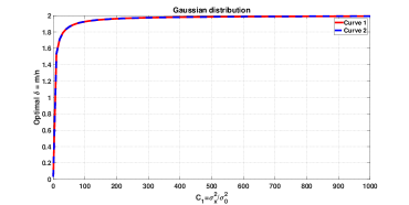
Figure 3: Gaussian case: Optimal $\delta$ vs $C_{1}=\sigma_{x}^{2}/\sigma_{0}^{2}$. The red solid line (Curve 1) is directly achieved via (47) and the blue dashed line (Curve 2) is achieved via ${\rm argmin_{\delta}}{\rm Err}$ where ${\rm Err}$ is defined by (7).

The optimal $\delta^{\dagger}$ for the least-favorable distribution is given by (19). For a given $\epsilon$, we have a unique value of $M\left(\epsilon,\alpha^{\dagger}\right)$ to quantify $\delta^{\dagger}$. For the Bernoulli-Gaussian case, we need to try different values of $\sigma_{e}^{\infty}$ to satisfy the condition $\left(\sigma_{e}^{\infty}\right)^{4}=4\sigma_{0}^{2}{\rm Err}_{\infty}$, thus $\delta^{\dagger}$ is computed numerically. In order to obtain intuition into the values of $\delta^{\dagger}$ for different signals, we derive bounds on $\delta^{\dagger}$ for the Gaussian, Bernoulli-Gaussian and least-favorable distributions.

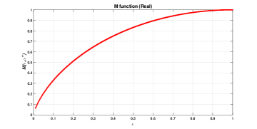
(a) Real case

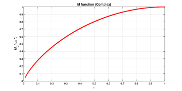
(b) Complex case

Figure 4: $M\left(\epsilon,\alpha^{\dagger}\right)$ vs $\epsilon$.

Proposition 3 (Gaussian Distribution).

For a linear measurement system (4) with our proposed Gaussian noise model (5), assume the signal elements are i.i.d. drawn from the Gaussian distribution as in Section II-C for both real and complex cases. Then $\delta^{\dagger}<2$. In addition, when $\sigma_{x}^{2}<2\sigma_{0}^{2}$, we have $\delta^{\dagger}<1$.

Proof:

We focus on (7) and replace $\sigma_{w}^{2}$ with $\delta\sigma_{0}^{2}$. Let $g(\delta)=\frac{f(\delta)}{\sigma_{0}^{2}}$ where

$$f(\delta) \coloneqq\left(-\delta^{2}\sigma_{0}^{2}+\left(1-\delta\right)\sigma_{x}^{2}\right)$$

$$+\sqrt{\left(\delta^{2}\sigma_{0}^{2}+\left(1-\delta\right)\sigma_{x}^{2}\right)^{2}+4\delta^{3}\sigma_{0}^{2}\sigma_{x}^{2}}.$$

Then

$$g(\delta) =\left(-\delta^{2}+\left(1-\delta\right)C_{1}\right)$$

$$+\sqrt{\left(\delta^{2}+\left(1-\delta\right)C_{1}\right)^{2}+4\delta^{3}C_{1}}$$

where $C_{1}=\frac{\sigma_{x}^{2}}{\sigma_{0}^{2}}$. Taking the derivative of $g(\delta)$ with respect to $\delta$ and equating it to zero results in $2C_{1}^{2}\delta^{2}+C_{1}^{3}\delta-2C_{1}^{3}=0$. We thus have two saddle points

$$\delta_{1}=\frac{-\sqrt{C_{1}^{2}+16C_{1}}-C_{1}}{4},\ \delta_{2}=\frac{\sqrt{C_{1}^{2}+16C_{1}}-C_{1}}{4}.$$

Since $\delta$ must be non-negative, we consider only $\delta_{2}$. In order to check whether $\delta_{2}$ is a minima, we rewrite $g(\delta)$ as

$$g(\delta) =\sqrt{\left(\delta^{2}+\left(1-\delta\right)C_{1}\right)^{2}+4\delta^{3}C_{1}}-\delta^{2}+\left(1-\delta\right)C_{1}$$

$$\geq\sqrt{\left(\delta^{2}+\left(1-\delta\right)C_{1}\right)^{2}+4\delta^{3}C_{1}}-\left(\delta^{2}+\delta C_{1}\right)$$

$$=\sqrt{\left(\delta^{2}+\delta C_{1}\right)^{2}+2C_{1}\delta^{2}-2C_{1}^{2}\delta+C_{1}^{2}}-\left(\delta^{2}+\delta C_{1}\right).$$

When $\delta\rightarrow\infty$, we have $2C_{1}\delta^{2}-2C_{1}^{2}\delta+C_{1}^{2}\rightarrow\infty$ which implies $g(\delta)\rightarrow\infty$, thus $\delta_{2}$ must be a local minima. The optimal number of measurements is then

$$\delta^{\dagger} =\delta_{2}=\frac{\sqrt{C_{1}^{2}+16C_{1}}-C_{1}}{4}$$ (47)

$$<\frac{\sqrt{C_{1}^{2}+16C_{1}+64}-C_{1}}{4}=\frac{\left(C_{1}+8\right)-C_{1}}{4}=2.$$

In addition, when

$$\sigma_{x}^{2}<2\sigma_{0}^{2},$$ (48)

we have $C_{1}<2$. Since (47) is a monotonically increasing function, the condition $C_{1}<2$ results in $\delta^{\dagger}<1$. ∎

The relationship between $\delta^{\dagger}$ and $C_{1}$ is simulated in Fig. 3. The red solid line (Curve 1) is calculated via (47) and the blue dashed line (Curve 2) is achieved via ${\rm argmin_{\delta}}{\rm Err}$ where ${\rm Err}$ is the function of (7).

Proposition 4 (Least-favorable Distribution).

For a linear measurement system (4) with our proposed Gaussian noise model (5), assume the signal elements are i.i.d. drawn from the least-favorable distribution as in Section IV for the real case and Section V for the complex case. Then $\delta^{\dagger}<2$. When $M(\epsilon,\alpha^{\dagger})<0.5$ for the real case and $M_{C}(\epsilon,\alpha^{\dagger})<0.5$ for the complex case, we have $\delta^{\dagger}<1$.

Proof:

Based on Theorem 1, we have $\delta^{\dagger}=2M(\epsilon,\alpha^{\dagger})$. In order to bound $\delta^{\dagger}$, we need to consider a bound on $M\left(\epsilon,\alpha\right)$.

We first treat the real case, in which we rewrite $M\left(\epsilon,\alpha\right)$ as

$$M\left(\epsilon,\alpha\right)=\epsilon T_{1}+T_{2},$$

where

$$T_{1} =\left(1+\alpha^{2}\right)+2\alpha\phi\left(\alpha\right)-2\left(1+\alpha^{2}\right)\Phi\left(-\alpha\right),$$

$$T_{2} =2\left(1+\alpha^{2}\right)\Phi\left(-\alpha\right)-2\alpha\phi\left(\alpha\right).$$

For any $\alpha\geq 0$, we have $\Phi\left(-\alpha\right)\leq\frac{1}{2}$. Thus,

$$T_{1} =\left(1+\alpha^{2}\right)+2\alpha\phi\left(\alpha\right)-2\left(1+\alpha^{2}\right)\Phi\left(-\alpha\right)$$

$$\geq\left(1+\alpha^{2}\right)-2\left(1+\alpha^{2}\right)\Phi\left(-\alpha\right)$$

$$=\left(1+\alpha^{2}\right)\left(1-2\Phi\left(-\alpha\right)\right)\geq 0$$

which means that for any fixed $\alpha\geq 0$, $M\left(\epsilon,\alpha\right)$ is a monotonically increasing function. Thus, for any $0<\epsilon_{1}<\epsilon_{2}\leq 1$, we have $M(\epsilon_{1},\alpha)<M(\epsilon_{2},\alpha)\leq M\left(1,\alpha\right)$, where,

$$M\left(1,\alpha\right)=1+\alpha^{2}.$$

Let $\alpha_{1}^{\dagger}$ be the optimal value that minimises $M\left(1,\alpha\right)$. Then $M(1,\alpha_{1}^{\dagger})=1$ and for any fixed $\alpha_{1}^{\dagger}$, $M(\epsilon,\alpha_{1}^{\dagger})$ is a monotonically increasing function as mentioned above, which means $M(\epsilon_{1},\alpha_{1}^{\dagger})<M(1,\alpha_{1}^{\dagger})$. Let $\alpha_{\epsilon_{1}}^{\dagger}$ be the optimal value that minimises $M(\epsilon_{1},\alpha)$. Then $M(\epsilon_{1},\alpha_{\epsilon_{1}}^{\dagger})\leq M(\epsilon_{1},\alpha_{1}^{\dagger})<1$ which means $M(\epsilon,\alpha^{\dagger})$ is upper bounded by $1$ and $\delta^{\dagger}=2M\left(\epsilon,\alpha^{\dagger}\right)$ is upper bounded by $2$. Furthermore, for $M(\epsilon,\alpha^{\dagger})<0.5$, we have $\delta^{\dagger}<1$ which only depends on $\epsilon$.

For the complex case, the analysis is similar. We rewrite (38) as $M_{C}\left(\epsilon,\alpha\right)=\epsilon T_{1}+T_{2}$ where

$$T_{1} =1+\alpha^{2}-\sqrt{2\pi}\phi\left(\sqrt{2}\alpha\right)+2\alpha\sqrt{\pi}\Phi\left(-\sqrt{2}\alpha\right),$$

$$T_{2} =\sqrt{2\pi}\phi\left(\sqrt{2}\alpha\right)-2\alpha\sqrt{\pi}\Phi\left(-\sqrt{2}\alpha\right).$$

For any given $\alpha\geq 0$, we have

$$T_{1} \geq 1+\alpha^{2}-\sqrt{2\pi}\phi\left(\sqrt{2}\alpha\right)$$

$$=1+\alpha^{2}-{\rm exp}\left(-\alpha^{2}\right)\geq 0.$$

By following the analysis in the real case, the same bound is achieved. ∎

To actually determine $\delta^{\dagger}$, we rely on numerical evaluations. For any given $\epsilon$, there are no closed form formulas to compute $\alpha^{\dagger}$ in (16) and $M\left(\epsilon,\alpha^{\dagger}\right)$ in (20): they have to be obtained numerically. As a consequence, for any given value of $M\left(\epsilon,\alpha^{\dagger}\right)$, the corresponding $\epsilon$ has to be found numerically. Simulations in Fig. 4 show that for both real and complex cases, $M\left(\epsilon,\alpha^{\dagger}\right)$ is upper bounded by 1, and $\epsilon$ should be smaller (approximately) than $0.1928$ for the real case and $0.2289$ for the complex case to achieve $\delta^{\dagger}<1$.

Proposition 5 (Bernoulli-Gaussian Distribution).

For a linear measurement system (4) with our proposed Gaussian noise model (5), assume the signal elements are i.i.d. drawn from the Bernoulli-Gaussian distribution as in Section IV for the real case and Section V for the complex case. Then $\delta^{\dagger}<2$ and when $\sigma_{x}^{2}<\frac{1}{\epsilon(1-R^{\infty}I\left(R^{\infty},\epsilon\right))}\sigma_{0}^{2}$ for the real case and $\sigma_{x}^{2}<\frac{1}{\epsilon(1-R^{\infty}I_{C}\left(R^{\infty},\epsilon\right))}\sigma_{0}^{2}$ for the complex case, we have $\delta^{\dagger}<1$.

Proof:

Based on Section IV-B we known that

$$\delta^{\dagger}=\frac{\left(\sigma_{e}^{\infty}\right)^{2}}{2\sigma_{0}^{2}}$$ (49)

with the constraint $\left(\sigma_{e}^{\infty}\right)^{4}=4\sigma_{0}^{2}{\rm Err}_{\infty}\left(\epsilon\right)$. For a fixed $\sigma_{0}^{2}$, we have $\delta^{\dagger}\propto\left(\sigma_{e}^{\infty}\right)^{2}\propto 2\sigma_{0}\sqrt{{\rm Err}_{\infty}\left(\epsilon\right)}$, thus we need to find the bound on ${\rm Err}_{\infty}\left(\epsilon\right)$ (here we use ${\rm Err}_{\infty}\left(\epsilon\right)$ instead of ${\rm Err}_{\infty}$ to highlight that ${\rm Err}_{\infty}\left(\epsilon\right)$ is a function of $\epsilon$).

Recall (26) which can be rewritten as

$${\rm{\rm Err}_{\infty}}\left(\epsilon\right)=\sigma_{x}^{2}\epsilon-\sigma_{x}^{2}R^{\infty}I\left(R^{\infty},\epsilon\right)\epsilon$$ (50)

where $I\left(R^{\infty},\epsilon\right)$ is given by (24). For any given $R^{\infty}$ in (23) (which depends on $\sigma_{x}^{2}$ and $\sigma_{e}^{\infty}$ ), let $0<\epsilon_{1}<\epsilon_{2}\leq 1$. It is easy to verify that

$$0<I\left(R^{\infty},\epsilon_{1}\right)<I\left(R^{\infty},\epsilon_{2}\right)\leq 1.$$

Define $f_{1}(\epsilon)\coloneqq\sigma_{x}^{2}\epsilon$ and $f_{2}\left(\epsilon\right)\coloneqq\sigma_{x}^{2}R^{\infty}I\left(R^{\infty},\epsilon\right)\epsilon$. Then

$$\frac{f_{1}(\epsilon)}{f_{2}\left(\epsilon\right)}=\frac{1}{R^{\infty}I\left(R^{\infty},\epsilon\right)}\geq 1$$

which means that ${\rm{\rm Err}_{\infty}}\left(\epsilon\right)$ is a monotonically increasing function of $\epsilon$ for any given $\sigma_{x}^{2},$ $\sigma_{e}^{\infty}$ and $\sigma_{0}^{2}$. Thus for $0<\epsilon_{1}<\epsilon_{2}\leq 1$, we have

$$0<{\rm Err}_{\infty}(\epsilon_{1})<{\rm Err}_{\infty}(\epsilon_{2})\leq{\rm Err}_{\infty}(1)$$

and for $\epsilon=1$, the Bernoulli-Gaussian distribution degenerates to the Gaussian signal. Thus ${\rm Err}_{\infty}\left(\epsilon\right)$ in the Bernoulli-Gaussian case is upper bounded by the Gaussian case, in other words, $\delta^{\dagger}$ is upper bounded by $2$.

Consider the following condition

$$\sigma_{x}^{2}<\frac{1}{\epsilon(1-R^{\infty}I\left(R^{\infty},\epsilon\right))}\sigma_{0}^{2}.$$ (51)

Based on (50) we have

$${\rm{\rm Err}_{\infty}}\left(\epsilon\right) <\sigma_{0}^{2}.$$

Multiplying $4\sigma_{0}^{2}$ on both sides gives

$$4\sigma_{0}^{2}{\rm Err}_{\infty}\left(\epsilon\right) <4\sigma_{0}^{4}.$$ (52)

For $\delta^{\dagger}$ we have the equality constraint $\left(\sigma_{e}^{\infty}\right)^{4}=4\sigma_{0}^{2}{\rm Err}_{\infty}\left(\epsilon\right)$. Substituting $\left(\sigma_{e}^{\infty}\right)^{4}=4\sigma_{0}^{2}{\rm Err}_{\infty}\left(\epsilon\right)$ into (52) results in

$$\frac{\left(\sigma_{e}^{\infty}\right)^{4}}{4\sigma_{0}^{4}} <1.$$

Taking the square root of both sides and only considering the real value, we achieve the specific region

$$\delta^{\dagger}=\frac{\left(\sigma_{e}^{\infty}\right)^{2}}{2\sigma_{0}^{2}}<1.$$

The same analysis holds in the complex case. ∎

Currently, there is no simple closed-form expression to describe the relationship between $\sigma_{0}^{2}$, $\sigma_{x}^{2}$, $\epsilon$ and $\left(\sigma_{e}^{\infty}\right)^{2}$. Simulation of the specific region $\delta^{\dagger}<1$ is provided in Fig. 5, where $\delta^{\dagger}$ is calculated via (49). Here we set $\sigma_{x}^{2}=1$ and try different values of $\sigma_{e}^{\infty}$ such that $\left|\left(\sigma_{e}^{\infty}\right)^{4}-4\sigma_{0}^{2}{\rm Err}_{\infty}\right|<10^{-6}$, after which we compute $\delta^{\dagger}=\frac{\left(\sigma_{e}^{\infty}\right)^{2}}{2\sigma_{0}^{2}}$ to find the optimal value. For the case $\epsilon=1$, we found $\delta^{\dagger}=1$ when $\sigma_{0}^{2}=0.5$ which coincides with the results from Fig. 2b.

VI-B Numerical Justification

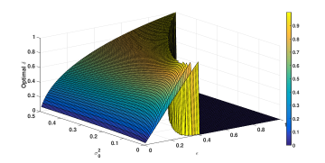
(a) 3D plot (real case)

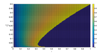
(b) 2D plot (real case)

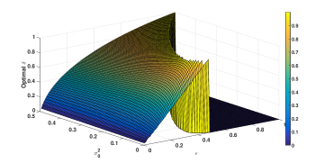
(c) 3D plot (complex case)

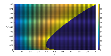
(d) 2D plot (complex case)

Figure 5: Simulation of $\delta^{\dagger}$ with respect to $\sigma_{0}^{2}$ and $\epsilon$ with fixed value $\sigma_{x}^{2}=1$. Only the specific region $\delta^{\dagger}<1$ is plotted.

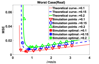
(a)

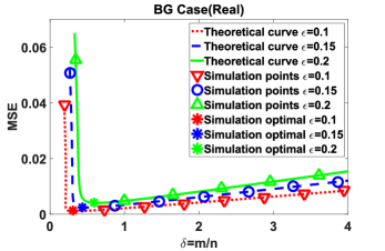
(b)

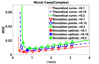
(c)

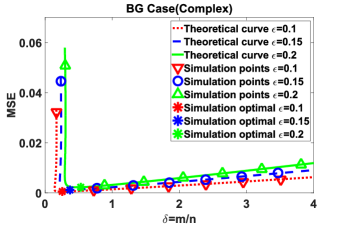
(d)

Figure 6: MSE (${\rm Err}_{\infty}$) vs $\delta$.

Both the theorems provided in Section IV and the bounds in Section VI rely heavily on the SE technique of the AMP algorithm. We compare the practical curves of the MSE of AMP and the theoretical curves achieved by SE.

For the simulation, we set $n=1000$, $\sigma_{0}^{2}=0.01$ as constant values. For the Bernoulli-Gaussian signal, we let $\sigma_{x}^{2}=1$, and for the least-favorable signal, we use a Bernoulli-Gaussian distribution but with large variance $\sigma_{x}^{2}=100$. Each simulation point is the average of $100$ independent trials.

The simulation results provided in Fig. 6 show the relationship between the MSE and the measurement ratio $\delta$ for a given normalised sparsity level $\epsilon=\frac{S}{n}$. From the figure, one can observe that when $\delta$ increases, the MSE decreases dramatically until it reaches a minimum. After that, further increase in $\delta$ increases the MSE. This phenomenon verifies our presumption that there exists an optimal $\delta^{\dagger}$ (or $m^{\dagger}$) for an energy fixed signal transmission system.

The overall performance of the Bernoulli-Gaussian distribution is better than the least-favorable distribution. The numerical results of the Bernoulli-Gaussian signal match the theoretical curves quite well but for the least-favorable distribution, the numerical results (MSE) are slightly larger than the theoretical curves. The main reason is that for the theoretical analysis in this case, we assume that the values of the non-zero coefficients are $\pm\infty$, but in simulations, these values can only be set as certain large numbers which results in a lower SNR compared with the one in the theoretical case. For both signal distributions, the trends of $\delta^{\dagger}$ for different $\epsilon$ values coincides with our theoretical analysis.

VII Conclusions

In this paper, we study the quadratically decreasing SNR setting by assuming an energy limited system with a noise model whose variance is proportional to the number of measurements. Analyses via random matrix theory and state evolution both show there exists an optimal choice of number of measurements to minimise the MSE of the estimated signal. The obtained conclusion is quit different from the traditional case which usually suggests the more measurements the better. Bounds on the optimal value $\delta=\frac{m}{n}$ for three commonly used signal distributions, Gaussian, Bernoulli-Gaussian and least-favorable, show that in both the real and complex domains, the optimal value $\delta$ is upper bounded by the value of 2. Specific situations in which $\delta^{\dagger}<1$ for the three signal models have also been analysed.

-A $\eta$ and ${\rm Err}_{t}$ for Bernoulli-Gaussian Prior (Real)

In this section, we provide the derivations of (25) and (26) in the real domain.

Assume the following scalar equation

$$\beta=x+w_{e}$$ (53)

where $x$ has density function (22) and $w_{e}$ is the noise with density $\mathcal{N}\left(0,\sigma_{e}^{2}\right)$. The joint probability of $x$ and $\beta$ is

$$p\left(x,\beta\right)= p_{G}\left(\beta-x;\,0,\,\sigma_{e}^{2}\right)\left(1-\epsilon\right)\Delta_{x=0}$$

$$+\epsilon p_{G}\left(\beta-x;\,0,\,\sigma_{e}^{2}\right)p_{G}\left(x;\,0,\,\sigma_{x}^{2}\right)$$

and

$$p\left(\beta\right)=\left(1-\epsilon\right)p_{G}\left(\beta;\,0,\,\sigma_{e}^{2}\right)+\epsilon p_{G}\left(\beta;\,0,\,\sigma_{x}^{2}+\sigma_{e}^{2}\right).$$

Let the estimation be $\hat{x}=\eta\left(\beta\right)={\rm E}_{x|\beta}\left[x|\beta\right]$. Based on Bayes’ theorem, we have

$$\hat{x} =\int x\frac{p\left(x,\beta\right)}{p\left(\beta\right)}dx$$

$$=\frac{\int xp_{G}\left(\beta-x;\,x,\,\sigma_{e}^{2}\right)p_{G}\left(x;0,\,\sigma_{x}^{2}\right)dx}{\frac{\left(1-\epsilon\right)}{\epsilon}p_{G}\left(\beta;\,0,\,\sigma_{e}^{2}\right)+p_{G}\left(\beta;\,0,\,\sigma_{x}^{2}+\sigma_{e}^{2}\right)}.$$ (54)

We next rely on the following lemma.

Lemma 6.

Let $\bm{y}=\bm{A}\bm{x}+\bm{w}$ where $\bm{A}\in\mathbb{R}^{m\times n}$ is a deterministic matrix, $\bm{x}\sim\mathcal{N}\left(\bm{0},\bm{\Sigma}_{x}\right)$ and $\bm{w}\sim\mathcal{N}\left(\bm{0},\bm{\Sigma}_{w}\right)$ are Gaussian random vectors. Assume all the matrix inverses exist. Then

$$\bm{\mu}_{\bm{x}|\bm{y}} =\bm{\Sigma}_{x}\bm{A}^{T}\left(\bm{A}\bm{\Sigma}_{x}\bm{A}^{T}+\bm{\Sigma}_{w}\right)^{-1}\bm{y}$$

$$=\left(\bm{\Sigma}_{x}^{-1}+\bm{A}^{T}\bm{\Sigma}_{w}^{-1}\bm{A}\right)^{-1}\bm{A}^{T}\bm{\Sigma}_{w}^{-1}\bm{y},$$

$$\bm{\Sigma}_{\bm{x}|\bm{y}} =\left(\bm{\Sigma}_{x}^{-1}+\bm{A}^{T}\bm{\Sigma}_{w}^{-1}\bm{A}\right)^{-1}$$

$$=\bm{\Sigma}_{x}-\bm{\Sigma}_{x}\bm{A}^{T}\left(\bm{A}\bm{\Sigma}_{x}\bm{A}^{T}+\bm{\Sigma}_{w}\right)^{-1}\bm{\Sigma}_{x}$$

where $\bm{\mu}_{\bm{x}|\bm{y}}$ is the conditional mean and $\bm{\Sigma}_{\bm{x}|\bm{y}}$ is the conditional covariance matrix.

Consider the mean value $\bm{\mu}_{\bm{x}|\bm{y}}$ in Lemma 6, which is used to compute ${\rm E}_{\bm{x}|\bm{y}}\left[\bm{x}|\bm{y}\right]$. Now apply this result to the scalar function (53). By setting $\epsilon=1$, we have the following fact

$$\frac{\int xp_{G}\left(\beta-x;\,x,\,\sigma_{e}^{2}\right)p_{G}\left(x;0,\,\sigma_{x}^{2}\right)dx}{p_{G}\left(\beta;\,0,\,\sigma_{x}^{2}+\sigma_{e}^{2}\right)} =R\beta,$$ (55)

where $R\coloneqq\frac{\sigma_{x}^{2}}{\sigma_{x}^{2}+\sigma_{e}^{2}}$. Substituting (55) into (54) provides

$$\hat{x} =\frac{p_{G}\left(\beta;\,0,\,\sigma_{x}^{2}+\sigma_{e}^{2}\right)\epsilon R\beta}{\left(1-\epsilon\right)p_{G}\left(\beta;\,0,\,\sigma_{e}^{2}\right)+\epsilon p_{G}\left(\beta;\,0,\,\sigma_{x}^{2}+\sigma_{e}^{2}\right)}$$

$$=\frac{p_{G}\left(\beta;\,0,\,\sigma_{x}^{2}+\sigma_{e}^{2}\right)\epsilon R\beta}{p\left(\beta\right)}$$

which has the same form as (25).

Now consider the MSE as ${\rm Err}={\rm E}\left[\left(x-\hat{x}\right)^{2}\right]$. Thus

$${\rm Err} ={\rm E}\left[x^{2}-2{\rm E}_{x|\beta}\left[x|\beta\right]x+{\rm E}_{x|\beta}\left[x|\beta\right]^{2}\right]$$

$$={\rm E}_{\beta}\left[{\rm E}_{x|\beta}\left[x^{2}-2{\rm E}_{x|\beta}\left[x|\beta\right]x+{\rm E}_{x|\beta}\left[x|\beta\right]^{2}\right]\right]$$

$$={\rm E}_{\beta}\left[{\rm E}_{x|\beta}\left[x^{2}|\beta\right]\right]-{\rm E}_{\beta}\left[{\rm E}_{x|\beta}\left[x|\beta\right]^{2}\right].$$

Note that ${\rm E}_{\beta}\left[{\rm E}_{x|\beta}\left[x^{2}|\beta\right]\right]={\rm E}\left[x^{2}\right]=\epsilon\sigma_{x}^{2}$ based on the law of total expectation. For ${\rm E}_{\beta}\left[{\rm E}_{x|\beta}\left[x|\beta\right]^{2}\right]$ we have

$${\rm E}_{\beta}\left[{\rm E}_{x|\beta}\left[x|\beta\right]^{2}\right]= \int\frac{p_{G}\left(\beta;\,0,\,\sigma_{x}^{2}+\sigma_{e}^{2}\right)^{2}\epsilon^{2}R^{2}\beta^{2}}{p\left(\beta\right)}d\beta$$

$$= \epsilon\sigma_{x}^{2}R\int\frac{\frac{1}{\sigma_{x}^{2}+\sigma_{e}^{2}}p_{G}\left(\beta;\,0,\,\sigma_{x}^{2}+\sigma_{e}^{2}\right)\beta^{2}}{\frac{\left(1-\epsilon\right)}{\epsilon}\frac{p_{G}\left(\beta;\,0,\,\sigma_{e}^{2}\right)}{p_{G}\left(\beta;\,0,\,\sigma_{x}^{2}+\sigma_{e}^{2}\right)}+1}d\beta.$$

Define $\beta\coloneqq\sqrt{\sigma_{x}^{2}+\sigma_{e}^{2}}\gamma$. Then

$${\rm E}_{\beta}\left[{\rm E}_{x|\beta}\left[x|\beta\right]^{2}\right]= \epsilon\sigma_{x}^{2}R\int\frac{\frac{1}{\sqrt{2\pi}}{\rm exp}\left(-\frac{\gamma^{2}}{2}\right)}{\frac{\left(1-\epsilon\right)}{\epsilon}\sqrt{\frac{1}{1-R}}{\rm exp}\left(-\frac{\gamma^{2}\sigma_{x}^{2}}{2\sigma_{e}^{2}}\right)+1}\gamma^{2}d\gamma$$

$$= \epsilon\sigma_{x}^{2}RI\left(R,\epsilon\right)$$

and

$${\rm Err} =\epsilon\sigma_{x}^{2}-\epsilon\sigma_{x}^{2}RI\left(R,\epsilon\right)$$

$$=\left[\frac{R\epsilon}{1-R}\left(1-RI\left(R,\epsilon\right)\right)\right]\sigma_{e}^{2}$$

which has the same form as (26).

-B $\eta$ and ${\rm Err}_{t}$ for Bernoulli-Gaussian Prior (Complex)

In this section, we extend (25) and (26) to the complex case. We start from (39). Following the same steps as in Appendix -A, we have

$$\hat{x} ={\rm E}\left[x|\beta\right]=\int xp\left(x|\beta\right)dx,$$

$$=\frac{p_{CG}\left(\beta;0,\sigma_{e}^{2}+\sigma_{x}^{2}\right)}{p_{C}\left(\beta\right)}\epsilon R\beta,$$

where

$$p_{C}\left(\beta\right)=\left(1-\epsilon\right)p_{CG}\left(\beta;0,\sigma_{e}^{2}\right)+\epsilon p_{CG}\left(\beta;0,\sigma_{e}^{2}+\sigma_{x}^{2}\right).$$

The MSE calculation in the complex case, becomes

$${\rm Err}_{C} ={\rm E}x^{2}-{\rm E}_{\beta}\left[\left|{\rm E}_{x|\beta}\left[x|\beta\right]\right|^{2}\right]$$

where we still have ${\rm E}x^{2}=\epsilon\sigma_{x}^{2}.$ The second term gives

$${\rm E}_{\beta}\left[\left|{\rm E}_{x|\beta}\left[x|\beta\right]\right|^{2}\right]$$

$$=\int\left|E_{x|\beta}\left[x|\beta\right]\right|^{2}p_{C}\left(\beta\right)d\beta$$ (56)

$$=\epsilon R^{2}\int_{\beta^{R}}\int_{\beta^{I}}\frac{p_{CG}\left(\beta;0,\sigma_{e}^{2}+\sigma_{x}^{2}\right)}{\frac{\left(1-\epsilon\right)}{\epsilon}\frac{p_{CG}\left(\beta;0,\sigma_{e}^{2}\right)}{p_{CG}\left(\beta;0,\sigma_{e}^{2}+\sigma_{x}^{2}\right)}+1}\left|\beta\right|^{2}d\beta^{R}d\beta^{I}.$$ (57)

In addition, we have $p_{CG}\left(x;0,\sigma_{x}^{2}\right)=\frac{1}{\sigma_{x}^{2}}\frac{1}{\pi}{\rm exp}\left(-\frac{\left|x\right|^{2}}{\sigma_{x}^{2}}\right)$.

Let $x=\sigma_{x}y$. Then,

$$p_{CG}\left(x;0,\sigma_{x}^{2}\right) =\frac{1}{\sigma_{x}^{2}}\frac{1}{\pi}{\rm exp}\left(-\frac{\sigma_{x}^{2}\left|y\right|^{2}}{\sigma_{x}^{2}}\right)$$

$$=\frac{1}{\sigma_{x}^{2}}\phi_{c}\left(y\right)=\frac{1}{\sigma_{x}^{2}}\phi_{c}\left(\frac{x}{\sigma_{x}}\right),$$

which implies that we can rewrite (57) as

$${\rm E}_{\beta}\left[\left|{\rm E}_{x|\beta}\left[x|\beta\right]\right|^{2}\right]$$

$$=\epsilon R^{2}\int_{\beta^{R}}\int_{\beta^{I}}\frac{\frac{1}{\sigma_{e}^{2}+\sigma_{x}^{2}}\phi_{c}\left(\frac{\beta}{\sqrt{\sigma_{e}^{2}+\sigma_{x}^{2}}}\right)}{\frac{\left(1-\epsilon\right)}{\epsilon}\frac{1}{1-R}{\rm exp}\left(-R\frac{\left|\beta\right|^{2}}{\sigma_{e}^{2}}\right)+1}\left|\beta\right|^{2}d\beta^{R}d\beta^{I}.$$ (58)

Define $\beta\coloneqq\sqrt{\sigma_{x}^{2}+\sigma_{e}^{2}}\gamma$. We then have $d\beta^{R}=\sqrt{\sigma_{e}^{2}+\sigma_{x}^{2}}d\gamma^{R}$ , $d\beta^{I}=\sqrt{\sigma_{e}^{2}+\sigma_{x}^{2}}d\gamma^{I}$, and $\left|\beta\right|^{2}=\left(\sigma_{e}^{2}+\sigma_{x}^{2}\right)\left|\gamma\right|^{2}$. Substituting into (58) leads to

$${\rm Err}_{C}$$

$$=\epsilon\sigma_{x}^{2}$$

$$-\sigma_{x}^{2}\epsilon R\int_{\gamma^{R}}\int_{\gamma^{I}}\frac{\phi_{c}\left(\gamma\right)}{\frac{\left(1-\epsilon\right)}{\epsilon}\frac{1}{1-R}{\rm exp}\left(-\frac{R}{1-R}\left|\gamma\right|^{2}\right)+1}\left|\gamma\right|^{2}d\gamma^{R}d\gamma^{I},$$

$$=\epsilon\sigma_{x}^{2}\left(1-RI_{C}\left(R,\epsilon\right)\right)=\left[\frac{R\epsilon}{1-R}\left(1-RI_{C}\left(R,\epsilon\right)\right)\right]\sigma_{e}^{2}$$

which has the same form as (43).

References

- [1] Y. Lu, W. Dai, and Y. C. Eldar, “Optimal number of measurements for compressed sensing with quadratically decreasing SNR,” European Signal Processing Conf. (EUSIPCO), pp. 1319–1323, Aug, 2017.
- [2] Y. C. Eldar, "Sampling Theory: Beyond Bandlimited Systems", Cambridge University Press, Apr, 2015.
- [3] Y. C. Eldar and G. Kutyniok, "Compressed Sensing: Theory and Applications", Cambridge University Press, May, 2012.
- [4] Y.C. Pati, R. Rezaiifar, and P.S. Krishnaprasad, “Orthogonal matching pursuit: recursive function approximation with applications to wavelet decomposition,” Asilomar Conf. Signals, Systems and Computers, pp. 40–44 vol.1, Nov, 1993.
- [5] W. Dai and O. Milenkovic, “Subspace pursuit for compressive sensing signal reconstruction,” IEEE Trans. Inf. Theory, vol. 55, no. 5, pp. 2230–2249, May, 2009.
- [6] D. Needell and J. A. Tropp, “CoSaMP: Iterative signal recovery from incomplete and inaccurate samples,” Appl. Comput. Harmon. A., vol. 26, no. 3, pp. 301–321, 2009.
- [7] R. Tibshirani, “Regression shrinkage and selection via the LASSO,” J. Royal Stat. Soc. Series B, pp. 267–288, 1996.
- [8] D. L. Donoho, A. Maleki, and A. Montanari, “Message-passing algorithms for compressed sensing,” Proc. Nat. Acad. Sci. USA., vol. 106, no. 45, pp. 18914–18919, 2009.
- [9] K. Aberman and Y. C. Eldar, “Sub-Nyquist SAR via Fourier domain range-doppler processing,” IEEE Trans. Geosci. Remote Sens., vol. 55, no. 11, pp. 6228–6244, Nov, 2017.
- [10] D. Cohen and Y. C. Eldar, “Sub-Nyquist cyclostationary detection for cognitive radio,” IEEE Trans. Signal Process., vol. 65, no. 11, pp. 3004–3019, Jun, 2017.
- [11] X. Zhao and W. Dai, “On joint recovery of sparse signals with common supports,” IEEE Int. Symp. Information Theory (ISIT), pp. 541–545, Jun, 2015.
- [12] R. Baraniuk and P. Steeghs, “Compressive radar imaging,” IEEE Radar Conf., pp. 128–133, Mar, 2007.
- [13] C. R. Berger, B. Demissie, J. Heckenbach, P. Willett, and S. Zhou, “Signal processing for passive radar using OFDM waveforms,” IEEE J. Sel. Topics Signal Process., vol. 4, no. 1, pp. 226–238, Feb, 2010.
- [14] S. Som, L. C. Potter, and P. Schniter, “Compressive imaging using approximate message passing and a markov-tree prior,” Asilomar Conf. Signals, Systems and Computers, pp. 243–247, Nov, 2010.
- [15] U. S. Kamilov, S. Rangan, A. K. Fletcher, and M. Unser, “Approximate message passing with consistent parameter estimation and applications to sparse learning,” IEEE Trans. Inf. Theory, vol. 60, no. 5, pp. 2969–2985, May, 2014.
- [16] J. R. Pierce, “Physical sources of noise,” Proc. IRE, vol. 44, no. 5, pp. 601–608, May, 1956.
- [17] D. Zhang, A. K. Bhide, and A. Alvandpour, “Design of CMOS sampling switch for ultra-low power ADCs in biomedical applications,” NORCHIP, pp. 1–4, Nov, 2010.
- [18] Behzad Razavi, Design of analog CMOS integrated circuits, McGraw-Hill, 2001.
- [19] A. C. Ery and Y. C. Eldar, “Noise folding in compressed sensing,” IEEE Signal Process. Lett., vol. 18, no. 8, pp. 478–481, Aug, 2011.
- [20] M. A. Davenport, J. N. Laska, J. R. Treichler, and R. G. Baraniuk, “The pros and cons of compressive sensing for wideband signal acquisition: Noise folding versus dynamic range,” IEEE Trans. Signal Process., vol. 60, no. 9, pp. 4628–4642, Sep, 2012.
- [21] J. N. Laska and R. G. Baraniuk, “Regime change: Bit-depth versus measurement-rate in compressive sensing,” IEEE Trans. Signal Process., vol. 60, no. 7, pp. 3496–3505, Jul, 2012.
- [22] W. Dai and O. Milenkovic, “Information theoretical and algorithmic approaches to quantized compressive sensing,” IEEE Trans. Commun., vol. 59, no. 7, pp. 1857–1866, Jul, 2011.
- [23] D. L. Donoho, A. Maleki, and A. Montanari, “Supporting information to: Message-passing algorithms for compressed sensing,” Proc. Nat. Acad. Sci. USA., 2009.
- [24] Avionics Department, “Electronic warfare and radar systems engineering handbook,” A Comprehensive Handbook for Electronic Warfare and Radar Systems Engineers, Oct, 2013.
- [25] S. Aja-Fernández and A. Tristán-Vega, “A review on statistical noise models for magnetic resonance imaging,” LPI, ETSI Telecomunicacion, Universidad de Valladolid, Spain, Tech. Rep., 2013.
- [26] M. Bayati and A. Montanari, “The dynamics of message passing on dense graphs, with applications to compressed sensing,” IEEE Trans. Inf. Theory, vol. 57, no. 2, pp. 764–785, Feb, 2011.
- [27] A. Montanari, “Graphical models concepts in compressed sensing,” arXiv preprint arXiv:1011.4328, 2010.
- [28] C. Rush and R. Venkataramanan, “Finite sample analysis of approximate message passing algorithms,” IEEE Trans. Inf. Theory, vol. 64, no. 11, pp. 7264–7286, Nov, 2018.
- [29] Y. Lu and W. Dai, “Extended AMP algorithm for correlated distributed compressed sensing model,” IEEE Int. Conf. Digital Signal Processing (DSP), pp. 700–704, Oct, 2016.
- [30] Y. Lu and W. Dai, “Independent versus repeated measurements: a performance quantification via state evolution,” IEEE Int. Conf. Acoustics, Speech and Signal Processing (ICASSP), pp. 4653–4657, Mar, 2016.
- [31] S. Rangan, “Generalized approximate message passing for estimation with random linear mixing,” IEEE Int. Symp. Information Theory (ISIT), pp. 2168–2172, Jul, 2011.
- [32] F. Krzakala, M. Mezard, F. Sausset, Y. Sun, and L. Zdeborova, “Probabilistic reconstruction in compressed sensing: algorithms, phase diagrams, and threshold achieving matrices,” J. Stat. Mech. Theory Exp., vol. 2012, no. 08, pp. P08009, 2012.
- [33] A. Maleki, L. Anitori, Z. Yang, and R. G. Baraniuk, “Asymptotic analysis of complex LASSO via complex approximate message passing (CAMP),” IEEE Trans. Inf. Theory, vol. 59, no. 7, pp. 4290–4308, Jul, 2013.