Reconstructing non-equilibrium regimes of quantum many-body systems from the analytical structure of perturbative expansions

Abstract

We propose a systematic approach to the non-equilibrium dynamics of strongly interacting many-body quantum systems, building upon the standard perturbative expansion in the Coulomb interaction. High order series are derived from the Keldysh version of determinantal diagrammatic Quantum Monte Carlo, and the reconstruction beyond the weak coupling regime of physical quantities is obtained by considering them as analytic functions of a complex-valued interaction $U$. Our advances rely on two crucial ingredients: i) a conformal change of variable, based on the approximate location of the singularities of these functions in the complex $U$-plane; ii) a Bayesian inference technique, that takes into account additional known non-perturbative relations, in order to control the amplification of noise occurring at large $U$. This general methodology is applied to the strongly correlated Anderson quantum impurity model, and is thoroughly tested both in- and out-of-equilibrium. In the situation of a finite voltage bias, our method is able to extend previous studies, by bridging with the regime of unitary conductance, and by dealing with energy offsets from particle-hole symmetry. We also confirm the existence of a voltage splitting of the impurity density of states, and find that it is tied to a non-trivial behavior of the non-equilibrium distribution function. Beyond impurity problems, our approach could be directly applied to Hubbard-like models, as well as other types of expansions.

I Introduction

The study of the out-of-equilibrium regime of strongly correlated many-body quantum problems is a major challenge in theoretical condensed matter physics. Its interest has grown rapidly in the past few years with new experiments, e.g. the ability to control light-matter interaction on ultra-fast time scaleFörst et al. (2011), light-induced superconductivity Fausti et al. (2011); Nicoletti et al. (2014); Casandruc et al. (2015); Nicoletti and Cavalleri (2016); Nicoletti et al. (2018) or metal-insulator transition driven by electric field Nakamura et al. (2013), proposed e.g. to build artificial neuronsdel Valle et al. (2018). These experiments raise the question whether the combination of strong correlation effects and out of equilibrium regimes could lead to genuinely new physics and phases of matter that do not have an equilibrium counterpart. Quantum nanoelectronics also provide many examples of such systems. A classic example is the spin-1/2 Kondo effect occurring in a quantum dot, but recent experiments have also managed to study in great detail underscreened Roch et al. (2009); Parks et al. (2010) and overscreened Iftikhar et al. (2015, 2018) (multi-channel) Kondo effects, characterized by non-Fermi liquid fixed points. Other notable examples of new quantum states induced by interactions are Luttinger liquidsGiamarchi (2004) that take place at edges in the fractional quantum Hall regime, or the “0.7 anomaly”Thomas et al. (1996, 1998); Micolich (2011) occurring in a simple quantum point contact geometry. Last, solid state based quantum computers such as spin qubits devices are nothing but out-of-equilibrium quantum many-body systems (few sites Hubbard like models, possibly connected to electrodes) that bring new questions into the scope of correlated systemsPreskill (2018).

It is worth noting that even the simplest of these out-of-equilibrium problems, the single impurity Anderson model, is still the subject of active researchReininghaus et al. (2014); Schwarz et al. (2018). Early approaches used a range of approximate techniques including 4th order perturbation theoryFujii and Ueda (2003), equation of motion techniquesVan Roermund et al. (2010) and the Non Crossing Approximation (NCA)Wingreen and Meir (1994). State of the art techniques include the time-dependent Numerical Renormalization Group (NRG) and the density matrix renormalization group (DMRG)White (1992, 1993); Schollwöck (2005); Anders and Schiller (2005); Heidrich-Meisner et al. (2009); Schwarz et al. (2018); Eckel et al. (2010). Early attempts of real time quantum Monte Carlo Mühlbacher and Rabani (2008); Werner et al. (2009, 2010); Schiró and Fabrizio (2009); Schiró (2010) have experienced an exponential sign problem at long time and large interaction. Within Monte-Carlo methods, two main routes are currently explored to resolve this issue: the inchworm algorithm Cohen et al. (2014a, b, 2015); Chen et al. (2017a, b) and the Schwinger-Keldysh diagrammatic Quantum Monte Carlo Profumo et al. (2015) (QMC). The later, which we use in this paper, reaches the infinite time steady state limit and has a complexity which does not grow with time. The development of controlled computational methods is critical for the development of the theory in this field. Beyond its direct application to impurities and quantum dot physics, the Anderson model is of direct interest for quantum embedding methods such as Dynamical Mean Field Theory Georges et al. (1996); Kotliar et al. (2006); Aoki et al. (2014) (DMFT) which reduce bulk lattice problem to the solution of a self-consistent quantum impurity model.

A straightforward approach to study out-of-equilibrium many-body quantum problem is to compute the systematic perturbative expansion of some physical quantity $F$ in power of the electron-electron interaction $U$: $F(U)\equiv\sum_{n=0}^{\infty}F_{n}U^{n}$. In practice, $F$ may depend on time (or frequency) as well as voltage-bias, temperature, etc. The coefficients $F_{n}$ are given by the out-of-equilibrium Schwinger-Keldysh version of the Feynman diagramsRammer (2007). Such a perturbative expansion is a central tool in quantum mechanics and quantum field theory. In weak coupling theories, a few orders are sufficient to explain many physical phenomena, even quantitatively, as e.g. in Quantum Electrodynamics (QED). However, at intermediate or strong coupling, this approach faces two main challenges: (i) the computation of the coefficients for $n$ large enough and (ii) the reconstruction of the physical quantities as a function of $U$ from a finite number of coefficients.

Using the standard Wick theorem, an explicit expression of $F_{n}$ to order $n$ can be written as $n-$dimensional integrals. While the computation of $F_{n}$ can hardly been achieved analytically beyond a few orders, Quantum Monte-Carlo (QMC) algorithms known as “diagrammatic Monte-Carlo”Prokof’ev and Svistunov (1998); Mishchenko et al. (2000); Van Houcke et al. (2008); Prokof’ev and Svistunov (2007, 2008); Gull et al. (2010); Kozik et al. (2010); Pollet (2012); Van Houcke et al. (2012); Kulagin et al. (2013a, b); Gukelberger et al. (2014); Deng et al. (2015); Huang et al. (2016); Rossi et al. (2018a); Van Houcke et al. (2019) are able to compute a finite number of these coefficients $F_{n}$ for a general class of quantum many-body problems, in practice up to $8$ or $15$ depending on the model and the physical quantity. The first generation of these algorithms explicitly sampled the Feynman diagrams one by one with a complex Markov chain, moving from one diagram to another. A second generation of algorithms handles the diagrams collectively using combinations of determinants to cancel disconnected diagrams in physical quantities. This was achieved in the real time Schwinger-Keldysh formalismProfumo et al. (2015), and in the imaginary time Matsubara formalismRossi (2017); Moutenet et al. (2018); Simkovic and Kozik (2017); Rossi (2018).

The resummation of the series is a non-trivial mathematical task outside of the weak coupling regime, even with a perfect knowledge of the coefficients $F_{n}$. The issue comes from the finite radius of convergence of the series. When $U$ is larger than this radius, the truncated series to the first $N$-th terms does not converge with $N$ and some resummation technique must be used to compute $F(U)$. Moreover, there are two additional difficulties associated with numerical methods: i) only a finite number of coefficients $F_{n}$ can be computed since the computation cost is exponential in $n$ and ii) the $F_{n}$ are only known with a finite precision, typically of a few digits in QMC.

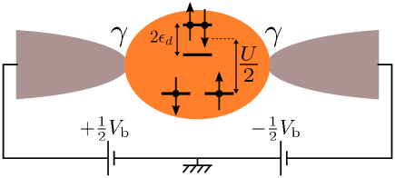
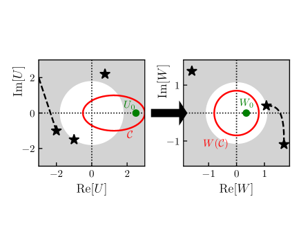
Figure 1: Upper panel: the Anderson quantum impurity model describing a single level quantum dot. The level with energy $\epsilon_{d}$ is subject to a finite Coulomb interaction $U$, and is hybridized with a tunnel coupling $\gamma$ to two leads that are biased with voltage $V_{b}$. Lower left panel: illustration of the general computation scheme developed in this work. A physical quantity $F$ (e.g. the current through the dot) presents singularities in the $U$ complex plane, such as poles (stars) or branch cuts (dashed line), hampering proper convergence of perturbative approaches for values of $U$ outside the convergence disk (grey area). After defining a broad singularity-free contour $\cal C$ (red line) that encircles both $U=0$ and a targeted $U_{0}$ value, a conformal map $U\to W(U)$ is defined in order to bring $W_{0}=W(U_{0})$ inside the convergence disk of $F[U(W)]$ (lower right panel). Resummation techniques can then be applied in a controlled way.

In this paper, we approach this problem from the angle of complex analysis. Indeed, the divergence of the series originates from the singularity structure of the function $F(U)$ in the complex plane $U$ (lower left panel in Fig. 1). We discuss how to locate the singularities closest to 0, and how to construct an analytic change of variable to resum the series beyond weak coupling (lower right panel in Fig. 1). We also introduce a Bayesian technique to take into account the amplification of the Monte-Carlo noise in the resummation process using some simple non-perturbative additional information on the model.

While our approach is quite general, we will focus here on the non-equilibrium Anderson quantum impurity model in the quantum dot configuration (upper panel in Fig. 1). Our starting point is an expansion of the Green’s function in power of the Hubbard interaction $U$, using an extension of the algorithm of Ref.Profumo et al. (2015). The algorithm is discussed in details in a companion paper Bertrand et al. (2019), its implementation is based on the TRIQS libraryParcollet et al. (2015). This algorithm provides a numerically exact computation of the perturbative series of physical quantities in power of the interaction $U$, at a cost which is uniform in time but exponential with the expansion order. Hence it allows to compute in a transient regime as well as directly in a long time steady state, a regime in which most competing methods have severe limitations.

This paper is organized as follows. Section II introduces our notations for the single impurity Anderson model. Section III develops the resummation technique and illustrates it on the Kondo temperature. Section IV performs a benchmark of the method against NRG for the equilibrium dynamics. Section V presents new results in the non-equilibrium regime, including the voltage-split spectral function, extended-range current-voltage characteristics, and a non-trivial dot distribution function. Section VI concludes this article and presents perspectives for our conformal approach to the perturbative expansions of strongly interacting quantum systems.

II The Anderson impurity model

In this paper, we focus on the single impurity Anderson model both at and out-of equilibrium. While originally formulated to describe the effect of magnetic impurities in metals, this model is widely used in theoretical condensed matter, both as a simple model for quantum dots in mesoscopic physics and as a building block of “quantum embedding” approximations like DMFT and its generalizations. At the core of the Anderson model lies Kondo physics. The repulsive interaction on the quantum dot leads to an effective antiferromagnetic interaction between the electronic reservoirs and the spin of the (unique) electron trapped in the quantum dot in the local moment regime. This interaction leads to the formation of the Kondo resonance, a thin peak in the local density of state pinned at the Fermi energyHewson (1993). The Anderson impurity Hamiltonian reads:

$$\hat{\mathrm{{\textbf{H}}}} = \sum_{i=-\infty}^{+\infty}\sum_{\sigma}\gamma_{i}\hat{\mathrm{{\textbf{c}}}}^{\dagger}_{i,\sigma}\hat{\mathrm{{\textbf{c}}}}_{i+1,\sigma}+h.c.+\epsilon_{d}(\hat{\mathrm{{\textbf{n}}}}_{\uparrow}+\hat{\mathrm{{\textbf{n}}}}_{\downarrow})$$ (1)

$$+U\theta(t)\left(\hat{\mathrm{{\textbf{n}}}}_{\uparrow}-\frac{1}{2}\right)\left(\hat{\mathrm{{\textbf{n}}}}_{\downarrow}-\frac{1}{2}\right).$$

It connects an impurity on site $0$ to two semi-infinite electrodes $i<0$ and $i>0$. The model corresponds to a single level artificial atom as sketched in the upper panel of Fig. 1. Here $\epsilon_{d}$ is the on-site energy of the impurity (relative to the particle-hole symmetric point), $\hat{\mathrm{{\textbf{n}}}}_{\sigma}=\hat{\mathrm{{\textbf{c}}}}^{\dagger}_{0,\sigma}\hat{\mathrm{{\textbf{c}}}}_{0,\sigma}$ is the impurity density of spin $\sigma$ electrons. $\hat{\mathrm{{\textbf{c}}}}^{\dagger}_{i,\sigma}$ and $\hat{\mathrm{{\textbf{c}}}}_{i,\sigma}$ are the creation and annihilation operators for electrons on site $i$ with spin $\sigma$. We use $\hbar=e=1$. $\theta(t)$ is the Heaviside function: We switch the interaction on at time $t=0$. Typical calculations will be performed for large times so that the system has relaxed to its stationary regime. The hopping parameters are given by $\gamma_{i}=1$ except for $\gamma_{0}=\gamma_{-1}=\gamma$ which connect the impurity to the electrodes. The calculations can be performed for arbitrary values of $\gamma$. However, since we are not interested in the large energy physics of the electrodes, we suppose that $\gamma\ll 1$, i.e. that the tunneling rate from the impurity to the electrodes is energy independent $\Gamma=2\pi\gamma^{2}\rho_{F}$ where $\rho_{F}$ is the density of states of the electron reservoirs at the Fermi level. The non-interacting retarded Green’s function of the free impurity is given by

$$g^{R}(\omega)=\frac{1}{\omega-\epsilon_{d}+i\Gamma}.$$ (2)

The two electrodes have a chemical potential symmetric with respect to zero $\pm V_{\rm b}/2$ which corresponds to a bias voltage $V_{\rm b}$. They share the same temperature that we take very low $T=10^{-4}\Gamma$. Within the standard non-equilibrium Keldysh formalism Stefanucci and van Leeuwen (2013), the non-interacting lesser and upper Green’s functions are given by:

$$g^{<}(\omega) = \frac{i\Gamma\left[n_{F}\left(\omega+\frac{V_{\rm b}}{2}\right)+n_{F}\left(\omega-\frac{V_{\rm b}}{2}\right)\right]}{(\omega-\epsilon_{d})^{2}+\Gamma^{2}},$$ (3)

$$g^{>}(\omega) = \frac{i\Gamma\left[n_{F}\left(\omega+\frac{V_{\rm b}}{2}\right)+n_{F}\left(\omega-\frac{V_{\rm b}}{2}\right)-2\right]}{(\omega-\epsilon_{d})^{2}+\Gamma^{2}},$$ (4)

where $n_{F}(\omega)=1/(e^{\omega/T}+1)$ is the Fermi function. $g^{>}(\omega)$ and $g^{<}(\omega)$ are the starting point for the expansion in power of $U$ that will be performed with real-time diagrammatic quantum Monte-Carlo.

The quantities of interest in this article are the interacting Green’s functions (denoted with capital letters),

$$G^{R}(t,t^{\prime}) = -i\theta(t-t^{\prime})\left<\left\{\hat{\mathrm{{\textbf{c}}}}_{0\uparrow}(t),\hat{\mathrm{{\textbf{c}}}}_{0\uparrow}^{\dagger}(t^{\prime})\right\}\right>,$$ (5a)

$$G^{<}(t,t^{\prime}) = i\left<\hat{\mathrm{{\textbf{c}}}}^{\dagger}_{0\uparrow}(t^{\prime})\hat{\mathrm{{\textbf{c}}}}_{0\uparrow}(t)\right>,$$ (5b)

$$G^{>}(t,t^{\prime}) = -i\left<\hat{\mathrm{{\textbf{c}}}}_{0\uparrow}(t)\hat{\mathrm{{\textbf{c}}}}_{0\uparrow}^{\dagger}(t^{\prime})\right>,$$ (5c)

where the operators have been written in Heisenberg representation. Since we will restrict ourselves to the stationary limit, these functions are a function of $t-t^{\prime}$ only and can be studied in the frequency domain. Of particular interest is the spectral function (or interacting local density of state) given by

$$A(\omega)=-\frac{1}{\pi}{\rm Im}[G^{R}(\omega)].$$ (6)

The equilibrium spectral function displays the important features of Kondo physics: a sharp Kondo resonance at the Fermi level, and satellite peaks around $\omega=\pm U/2$ in the case of particle-hole symmetry.

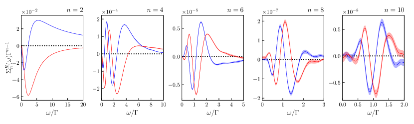
Figure 2: First non zero orders of the self-energy series $\Sigma^{R}(U,\omega)$ in powers of $U$ for the equilibrium particle-hole symmetric Anderson model (real part in blue, imaginary part in red). This series has been computed with a real-time diagrammatic quantum Monte-Carlo method detailed in a companion articleBertrand et al. (2019). The statistical error is shown as shaded areas. Due to particle-hole symmetry, odd orders are zeros.

The out of equilibrium spectral function can be used for the computation of the current-voltage characteristic using the Wingreen-Meir formulaMeir and Wingreen (1992),

$$I=\frac{\Gamma}{2}\int A(\omega)\left[n_{F}\left(\omega+\frac{V_{\rm b}}{2}\right)-n_{F}\left(\omega-\frac{V_{\rm b}}{2}\right)\right]d\omega.$$ (7)

The retarded self energy $\Sigma^{R}(\omega)$ is defined from the interacting Green’s function by:

$$G^{R}(\omega)=\frac{1}{\omega-\epsilon_{d}+i\Gamma-\Sigma^{R}(\omega)}.$$ (8)

Physical quantities have systematic expansion in power of $U$

$$G^{R}(t-t^{\prime})=\sum_{n=0}^{+\infty}G^{R}_{n}(t-t^{\prime})U^{n},$$ (9)

from which we obtain the corresponding quantity in the frequency domain by Fourier transform,

$$G^{R}(\omega)=\sum_{n=0}^{+\infty}G^{R}_{n}(\omega)U^{n}.$$ (10)

We obtain the functions $G^{R}_{n}(\omega)$ (typically up to $n=10$) using the QMC algorithm of Ref. Bertrand et al., 2019; Profumo et al., 2015. The expansion of the self-energy

$$\Sigma^{R}(\omega)=\sum_{n=0}^{+\infty}\Sigma^{R}_{n}(\omega)U^{n}$$ (11)

is obtained from the $G^{R}_{n}(\omega)$ using a formal series expansion order by order of the Dyson equation (8). As an illustration, Fig. 2 shows the self-energy series, up to order $10$, for the equilibrium particle-hole symmetric model as obtained from diagrammatic QMCBertrand et al. (2019). These series are the starting point of this paper, which is devoted to the resummation of the perturbative expansion for the Green’s function and the self-energy beyond weak coupling.

III The perturbative series beyond the weak coupling regime

Diagrammatic Quantum Monte Carlo yields the first orders of the perturbation expansion of physical quantities, with some error bars. In weak coupling, we can directly sum this series and obtain the physical quantities with a few orders. Beyond weak coupling however, we face a more complex problem. For a given physical quantity $F$, we want to evaluate $F(U)$ from the first $N$ (typically $N\sim 10$) coefficients $F_{0}$, $F_{1}$, $F_{2}$…$F_{N}$ of a series $F(U)\equiv\sum_{n=0}^{\infty}F_{n}U^{n}$. In the following, $F$ will stand for the width of the Kondo peak, the Green’s function $G$ or the self-energy $\Sigma$ of the impurity. In the latter cases, the coefficients are functions of the frequencies, $G_{n}(\omega)$ and $\Sigma_{n}(\omega)$. We also want to know, for a given physical quantity $F$ and interaction $U$, how many orders $N_{0}$ are needed to obtain $F(U)$ at a given precision. Since the cost of the diagrammatic QMC approach is exponential in $N_{0}$, the answer to this question gives the ultimate limit of the method.

The mathematical problem of series resummation is a quite old topic, e.g. Ref. Hardy, 1949. Various techniques have been used in physics problems including Padé approximants Baker and Graves-Morris (1996), Lindelöf extrapolationLindelöf (1905); Van Houcke et al. (2012) or Cesàro-Riesz techniqueProkof’ev and Svistunov (2008). In diagrammatic QMC, this is typically a post-processing step: the Monte-Carlo produces the values of the various orders of the expansion, and one then attempts to sum the series to obtain the final result. However, the situation is quite different if we want to use such technique to solve quantum impurity models in the context of the quantum embedding methods like DMFTGeorges et al. (1996), or e.g. TrilexAyral and Parcollet (2015); Ayral et al. (2017). Indeed, in such cases, the method require multiple solutions of impurity model to solve their self-consistency loop. Therefore, it is necessary to develop more robust methods to sum the perturbative series for impurity systems, which could be automatized.

In the cases considered in this paper (quantum impurity models), and in general for lattice models at finite temperature (such as the Hubbard model), the series for $F$ is expected to have a non-zero radius of convergence $R_{F}$. Note that $R_{F}$ not only depends on the chosen physical quantity $F$, but may also depend on frequency, voltage, temperature, etc. $R_{F}$ separates the weak coupling regime ($|U|<R_{F}$) from the strong coupling regime ($|U|>R_{F}$). At weak coupling, the truncated series $\sum_{n=0}^{N}F_{n}U^{n}$ provides an accurate estimate of $F(U)$ and is controlled exponentially with the number of coefficients $N$ (like a geometric series since $F_{n}\sim(1/R_{F})^{n}$). At strong coupling however, this truncated series diverges. Note that in some problems like e.g. the unitary fermionic gas, the series has a zero radius of convergence at zero temperature, see e.g. Ref. Rossi et al., 2018b for a recent example with diagrammatic QMC. We will not consider these cases in this paper, as they require other techniques as the ones presented here, e.g. Borel summation techniques.

In this paper, we consider the series summation problem with the angle of reconstructing the function $F(U)$ in the complex $U$ plane. The divergence of the series is due to the presence of singularities in the complex $U$ plane, starting on the circle $|U|=R_{F}$. The question is to reconstruct $F$ beyond the radius of convergence.

III.1 General theory

III.1.1 Conformal transformation

Conformal transformations can be used to deform the complex plane and bring the point to be computed back into the convergence disk of a transformed series. This technique was used a long time ago e.g. in statistical physics Guttmann (1989). In a previous workProfumo et al. (2015), some of us have shown that a simple conformal Euler transform allows to compute the density on the impurity up to $U=\infty$, at very low temperature, from the first 12 coefficients of the series. However, this Euler transform is not always successful in resumming other quantities like the Green’s function and the self-energy, and needs to be generalized.

Suppose that we aim at evaluating $F(U)$ at $U=U_{0}$ with $U_{0}$ real, positive and $U_{0}>R_{F}$. First, we assume a separation property, i.e. that we can find a simply connected domain delimited by a curve ${\cal C}$ containing 0 and $U_{0}$ but no singularities of the function $F$, as illustrated in the lower left panel of Fig. 1. The singularities of the function $F(U)$ will be located outside the domain ${\cal C}$. We then proceed as follows:

• First, according to the Riemann mapping theorem, we can construct a biholomorphic change of variable $W(U)$ such that i) $W(0)=0$, ii) it maps the interior of ${\cal C}$ into a disk $D_{\cal C}$ centered at $0$ in the $W$ plane (see the lower right panel in Fig. 1). In practice, we seek $\cal C$ to separate the singularities from the half straight line of real positive $U$. In the following, we will use two simple transformations, but in general we could use a Schwarz–Christoffel map if ${\cal C}$ is a polygon Driscoll and Trefethen (2002), composed with a Möbius transformation of the disk to enforce i) .

• Second, we form the series for the reciprocal function $U(W)$ of $W(U)$ which is defined term by term by the equation $U(W(U))=U$. We then construct the series $\bar{F}(W)\equiv\sum_{p}\bar{F}_{p}W^{p}$ defined by the composition $\bar{F}(W)=F(U(W))$. Since $W(0)=0$, the first $N$ terms of $F(W)$ can be computed from the first $N$ terms of $F(U)$.

• We evaluate the series $\bar{F}(W_{0})$ at the point of interest $W_{0}=W(U_{0})$. Indeed, by construction $W_{0}\in D_{\cal C}$ and, since $\bar{F}(W)$ is holomorphic in $D_{\cal C}$, $D_{\cal C}$ is included in the convergence disk of the series $\bar{F}$. Hence the series $\bar{F}$ converges at $W_{0}$.

The result is independent of the choice of the domain ${\cal C}$ but the speed of convergence of the series for $\bar{F}(W_{0})$ versus $N$ is not, since it is determined by the relative position of $W_{0}$ compared to the radius of convergence $R_{\bar{F}}$ of $\bar{F}$, i.e. $\eta_{{\cal C}}\equiv|W_{0}/R_{\bar{F}}|$. Therefore, there are ways to optimize the domain ${\cal C}$. For example, we can not simply take a narrow domain close to the real axis, for the convergence in $W$ would be really slow: we need to have $U_{0}$ and $0$ as “far” as possible from the curve ${\cal C}$ (the precise meaning of “far” being given by $\eta_{{\cal C}}$). For each domain ${\cal C}$ satisfying the separation property, there is a minimum number of orders $N_{{\cal C}}$ needed to obtain the result at a given precision $\epsilon$. There is therefore an optimal domain, which minimize $N_{{\cal C}}$ to $N_{opt}=\min_{{\cal C}}N_{{\cal C}}$. This is the absolute minimum of orders needed to sum the series, and therefore determine in fine the complexity of the diagrammatic QMC algorithm. Our next goal will be to approach such optimum.

Note that a failure of the separation assumption, i.e. the choice of a domain containing singularities, may result simply in the divergence of the series $\bar{F}$ at $W_{0}$, hence a clear failure of the method rather than a wrong result. Conversely the study of the convergence radius of the $\bar{F}(W)$ series provides direct information on the singularity free regions of the $U$ plane. Indeed, the region of the $U$ plane that maps towards the inside of the convergence radius of $\bar{F}(W)$ are singularity/branch cut free. Hence, using several conformal transforms, one may perform a step by step construction of the domain ${\cal C}$. Another note is that, as a consistency check, one can also check the stability of the final result upon small deformations of the domain (or the $W(U)$ function), as was discussed in details in Ref. Profumo et al., 2015 for the Euler transform.

The existence of the domain ${\cal C}$ and the transformation $W(U)$ has a direct consequence on the algorithmic complexity of diagrammatic Quantum Monte-Carlo. It was shown in Ref. Rossi, R. et al., 2017 that, for values of $U$ inside the convergence radius, connected diagrammatic quantum Monte-Carlo techniques provide a systematic route for calculating the many-body quantum problem in a computational time that only increases polynomially with the requested precision. The result also applies to the Keldysh diagrammatic QMC. For completeness, the core of the argument is as follows: inside the radius of convergence $R$, the precision of a calculation $\epsilon$ increases exponentially with the number of orders $N$ used $\epsilon\sim(U/R)^{N}$. Hence, although the computational time $C$ increases exponentially with $N$, $C\sim a^{N}$, the overall computational time scales as $C\sim(1/\epsilon)^{\log a/\log(R/U)}$, i.e. polynomially, see Ref. Rossi, R. et al., 2017 for a detailed analysis. For a given $U_{0}$ and domain ${\cal C}$, we now have to sum the transformed series $\bar{F}$ inside the radius of convergence. Hence the same argument also apply for this series, and therefore we conclude that, even outside the disk of convergence, we expect the algorithm to have a polynomial complexity as a function of the precision. Let us emphasize however that this result is largely academic, since in practice the power law can be large. Moreover, as we will discuss, for some physical quantities the transformation to $W$ can lead to a dramatic increase of the noise which induces a large computation time for a given precision.

III.1.2 Location of singularities in the complex $U$ plane

In order to choose ${\cal C}$ properly, we need to have some information on the location of the singularities in the $U$ plane. In this paper, we use the following technique to approximately locate the poles of $F(U)$ in the complex plane.

• We form an inverse of $F$ of the form $K(U)=1/(F(U)+a)$ as a formal series (i.e. order by order). $a$ is a constant that we choose at our convenience. In order for the series $K(U)$ to exist, we must have $F_{0}+a\neq 0$.

• We estimate the radii of convergence $R_{F}$ (resp. $R_{K}$) of $F$ (resp. $K$), by plotting $|F_{n}|$ and $|{K}_{n}|$ versus $n$, and fitting the asymptote $|F_{n}|\sim(1/R_{F})^{n}$

• In most of situations we found $R_{F}\neq R_{K}$. If not, we used a different $a$ so as to obtain $R_{F}\neq R_{K}$. Without loss of generality, let us assume that $R_{K}$ is the largest. We use the truncated polynomial of the series, $\sum_{p=0}^{N}{K}_{p}U^{p}$ to compute $K(U)$ within its disk of convergence and therefore locate its zeros, which are the poles of $F$. They will appear as the accumulation of the zeros of the polynomials at large enough $N$. If $R_{F}>R_{K}$, we simply reverse the roles of the series and reconstruct $K(U)$.

This technique has a quite large degree of generality, but also limitations. It assumes for example that the leading singularities in $F$ are poles and that the radius of convergence of $F$ and $K$ are different. Also it does not give us indications of poles that would be far from the origin but close to the real axis. However, in practice, we will see below that for the quantities and the physical problem considered in this paper (Green’s function and self-energy in real frequency, and Kondo temperature), this technique is sufficient. Finally, once $F(U)$ has been re-summed, it can be used to locate its zeros, hence for the resummation of $K(U)$ which provides another consistency check of the method.

III.1.3 Controlling the noise amplification using non-perturbative information and Bayesian inference

The transformation from $F_{n}$ to $\bar{F}_{p}$ is a linear one (with a lower triangular matrix), for a given transformation $W(U)$. Depending on the eigenvalues of the corresponding matrix, the Monte-Carlo error bar in $F_{n}$ may be strongly amplified by the transformation. As a result, the method may become unusable at strong coupling, as will be illustrated below on Fig. 6.

However, if we add some non-perturbative information, such as the fact that the Kondo temperature vanishes at infinite $U$, or a sum rule, we can construct a Bayesian inference technique that may be used to decrease the statistical uncertainty. Bayesian inference provides a systematic and rigorous way to incorporate this information into the results and improve their accuracy. In the rest of this paragraph, we describe the general theory for this technique. We will illustrate it in the following section.

Let us consider a series $F(U)=\sum_{n=0}^{N}F_{n}U^{n}$ where the $F_{n}$ are known with a finite precision. We note $F=\{F_{0},F_{1},\dots F_{N}\}$ the corresponding (vectorial) random variable. We calculate the mean values $\langle F_{n}\rangle$ and the corresponding errors $\delta_{n}$ within the quantum Monte-Carlo technique. We assume that the coefficients $F_{n}$ are given by independent Gaussian variables. This forms the “prior” distribution $P_{\rm prior}(F=f)$ in the absence of additional information.

$$P_{\rm prior}(F=f)=\prod_{i=0}^{N}\frac{1}{\sqrt{2\pi\delta_{n}}}e^{-\frac{(f_{n}-\langle F_{n}\rangle)^{2}}{2\delta_{n}^{2}}}$$ (12)

Let us note the additional information $X$. $X$ is a random variable that can be directly calculated from the series, $X=g(F)$ but whose actual value is also known very precisely by other means. In the example below, $X$ will be the value of $F(U)$ at large $U$. Bayesian inference amounts to replacing the prior distribution with the posterior distribution $P(F=f|X=x_{0})$ that incorporates the knowledge of the actual value of $X$ (we note $P(A|B)$ the conditional probability of event $A$ knowing event $B$). The value of $X$ is often known exactly. However, due to the presence of truncation errors, its value cannot be enforced exactly, and we suppose that it is known with a small error $\varepsilon$. Eventually, we take the limit $\varepsilon\rightarrow 0$. Hence, we assign to $X$ a Gaussian probability distribution $P_{X}(X=x)=1/(\varepsilon\sqrt{2\pi})\exp[-(x-x_{0})^{2}/(2\varepsilon^{2})]$ and define the posterior distribution as,

$$P_{\rm posterior}(F=f)\equiv\int dxP(F=f|X=x)P_{X}(X=x).$$ (13)

Using Bayes formula $P(F=f|X=x)=P(X=x|F=f)P_{\rm prior}(F=f)/P_{\rm prior}(X=x)$ and the deterministic relation $P(X=x|F=f)=\delta[x-g(f)]$, one arrives at,

$$P_{\rm posterior}(F=f)=\frac{P_{X}(X=g(f))P_{\rm prior}(F=f)}{P_{\rm prior}(X=g(f))}.$$ (14)

In practice, one proceeds as follows: (i) one generates many series according to $P_{\rm prior}(F=f)$. We emphasize that these series result from a single QMC run, hence are trivially generated (independent Gaussian numbers). Bayesian inference implies no significant computational overhead (ii) One construct a histogram of the values of $X$ to obtain $P_{\rm prior}(X=g(f))$. (iii) Each series is given a weight $P_{X}(X=g(f))/P_{\rm prior}(X=g(f))$ which is used to calculate other observables such as the value of $F(U)$ at different values of $U$. In practice the results are insensitive to the choice of $\varepsilon$ as long as it is chosen large enough so that a finite fraction of the sample contributes to the final statistics.

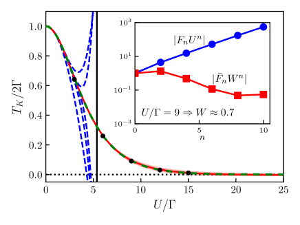
Figure 3: Resummation of the Kondo temperature (as defined in Eq. (15)) in the symmetric model ($\epsilon_{d}=0$). Plain red line: resummation technique including Bayesian inference, using the Euler transform (error bar shown as red shaded area); dashed thick green line: exact result from Bethe ansatzHorvatić, B. and Zlatić, V. (1985); black circles: reference NRG results; dashed blue lines: truncated series including up to $N=2,4,6,8$ and $10$ terms. The vertical line shows the estimated convergence radius of the series. Inset: evolution of $F_{n}U^{n}$ with $n$ for $U=9\Gamma$ in log-linear scale (blue circles); evolution of the series $\bar{F}_{n}W^{n}$ obtained after conformal transformation (red squares). The value $W=0.7$ is obtained by applying the conformal transformation to $U=9\Gamma$. The $\bar{F}_{n}W^{n}$ decreases exponentially, indicating convergence of the transformed series while the original series (blue circles) diverges.

III.2 Illustration with the Kondo temperature

Let us first apply the method described above to the Kondo temperature $T_{K}$ (which will be $F$ in this section). $T_{K}$ corresponds roughly to the width of the low energy Kondo peak, and is defined more specifically in this paper as the dimensionful Fermi liquid quasi-particle weight extracted from the retarded self-energy at low energy:

$$T_{K}(U)\equiv\frac{2\Gamma}{1-\left.\partial_{\omega}{\rm Re}\Sigma^{R}(U,\omega)\right|_{\omega=0}}.$$ (15)

Our first goal is to illustrate how the method actually works, and benchmark it against the calculation of the same quantity from the Numerical Renormalization Group (NRG) technique and Bethe ansatzHorvatić, B. and Zlatić, V. (1985).

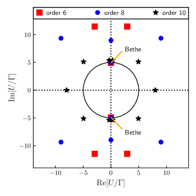
Figure 4: Poles of $T_{K}(U)$ identified from the zeros of the $1/T_{K}(U)$ function. These are found by looking for the zeros of its truncated series. Here they are shown in the $U/\Gamma$ complex plane with truncation at order 6 (red squares), 8 (blue points) and 10 (black stars). The black circle corresponds to $|U|=R_{T_{K}}$ where $R_{T_{K}}$ is the radius of convergence of the series of $T_{K}$. The stable points close to $\pm i5\Gamma$ correspond to true non-perturbative poles of $T_{K}(U)$. The exact zeros (small orange arrows) have been computed from the exact $1/T_{K}$ series found with Bethe ansatzHorvatić, B. and Zlatić, V. (1985).

III.2.1 Singularities in the complex $U$ plane

The dashed blue lines of Fig. 3 shows the truncated series of $T_{K}$ = $\sum_{n=0}^{N}F_{n}U^{n}$ for various orders $N\leq 10$. These truncated series diverge around $R_{T_{K}}\approx 5\Gamma$ which is the convergence radius of the series for these parameters. Increasing the value of $N$ helps to obtain a reliable value of $T_{K}$ closer to $R_{T_{K}}$. However, as expected, even with a very large number of terms, the bare series cannot be summed near or above $R_{T_{K}}$. Anticipating the final results, the plain red line corresponds to the results after resummation which matches very well what was obtained with our benchmark NRG calculation (see Sec. IV.1 for details on the used NRG implementation).

The inset of Fig. 3 shows the value of $|F_{n}U^{n}|$ (blue circles) as a function of $n$ for $U/\Gamma=9$ which lies above the convergence radius of the series. The log-linear plot shows an exponential increase of $|F_{n}U^{n}|\sim(U/R_{T_{K}})^{n}$ with $n$ which we use to extract the convergence radius of the series. Note that for other series, it can happen that $|F_{n}|$ oscillates with $n$. Whenever $F_{n}$ changes sign, it becomes close to zero which provides deviations from the clear exponential behaviour shown in the inset of Fig. 3. Hence, to obtain convergence radii which are robust to these outliers, we used a robust regression method on the $\log|F_{n}|$ versus $n$ data (we compute the regression slope as the median of all slopes between pairs of data points, this is known in statistics as the Theil-Sen estimatorTheil (1992)).

We now compute the first $10$ terms of the series of $1/T_{K}(U)$. This series has a radius of convergence of the order of $10\Gamma$. We look for the zeros, in the complex plane, of the series $1/T_{K}(U)$ truncated at order $N$. Since the truncated series is a polynomial, it has (generically) $N$ zeros, which are shown in Fig. 4 for $N=6$ (red squares), $N=8$ (blue circles) and $N=10$ (stars). One pair of zeros $U\approx\pm i5\Gamma$ is converged for all the truncations, hence corresponds to a true zero of $1/T_{K}(U)$, i.e. to a pole of $T_{K}(U)$. Fig. 4 also shows the circle $|U|=R_{T_{K}}$ extracted from the analysis of the $T_{K}(U)$ series done in the inset of Fig. 3. We find that the two poles $\pm i5\Gamma$ do indeed lie right on this circle.

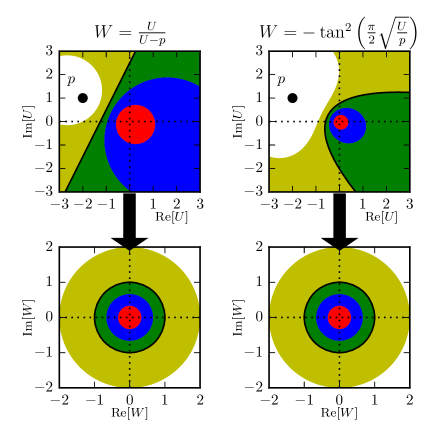
Figure 5: Left panels: Euler map. Right panels: parabola map. Upper panels: complex $U$ plane. Lower panels: complex $W$ plane. The transformation maps the upper regions of various colors onto the lower regions of matching colors. In particular the thick straight line (upper left) and the parabola (upper right) are mapped onto the unit circles (lower left and right respectively).

III.2.2 Conformal transformation

Let us now turn to the conformal transformation $W(U)$, which maps the two poles $\pm i5\Gamma$ away and brings the values of interest $U>0$ (real) closer to zero. We illustrate the technique with two maps: the Euler map defined by

$$W=\frac{U}{U-p},$$ (16)

and the “parabola” map which is defined as

$$W=-{\rm tan}^{2}\left(\frac{\pi}{2}\sqrt{\frac{U}{p}}\right),$$ (17)

where $p$ is an adjustable complex parameter.

Fig. 5 shows the various regions (different colors) in the $U$ plane that are mapped onto concentric circles of the $W$ plane. $0$ is mapped onto $0$ and $p$ onto $\infty$ in both transforms. The Euler map (left column) maps one half of the plane into the unit disk and the other half into the outside of the unit disk (separated by a black line). The parabola transform (right column) maps the inside of a parabola (black line) into the unit disk and the outside of the parabola into the outside of the unit disk. In the case where there are no singularities on the positive half plane ${\rm Re}[U]>0$, the Euler transform should be preferred since real values of $U>0$ are typically mapped closer to $U=0$ than with the parabola transform (compare the size of the blue region of the parabola and Euler case for instance). However, the parabola map is more agnostic about the positions of the singularities and will work even if there are singularities on the positive half plane ${\rm Re}[U]>0$ as long as they lie outside the parabola.

We now perform the resummation of $T_{K}(U)$. The series contains only even power of $U$ due to particle-hole symmetry, so that it can be considered as a function of $U^{2}$. The two poles $U=\pm i5\Gamma$ correspond to a single one $U^{2}=-25\Gamma^{2}$. In the $U^{2}$ plane, the pole being on the negative real axis, the Euler maps works very effectively. The resummation can also be performed with the parabola transform.

Once the conformal map is selected, we form the series $\bar{F}_{p}$ in the $W$ variable, as explained above. The inset of Fig. 3 shows $\bar{F}_{n}W_{0}^{n}$ (red squares) as a function of $n$ for $W_{0}=0.7=W(U_{0}=9\Gamma)$, using the Euler map with $p=-35\Gamma^{2}$ (the parabola yields similar results with $p=-15\Gamma^{2}$). As expected, $U_{0}$ is way beyond the radius of convergence in the original variable $U$, while $W_{0}$ lies within the disk of convergence of $\bar{F}(W)$ whose radius is found to be $R_{\bar{F}}\approx 2$. The final result $T_{K}(U)$ using the Euler transforms is shown in Fig. 3. The parabola transform (not shown) is undistinguishable from the Euler at this scale.

In this work, singularities were never found near the real positive axis, so that all $U>0$ can be reached using the conformal transforms of Fig. 5, given that enough orders of the series are known. However, one may very well build a conformal transform to reach a regime beyond a singularity by considering a concave contour $\cal C$, as it is shown in Appendix A. This may become interesting if a phase transition occurs when interaction is increased.

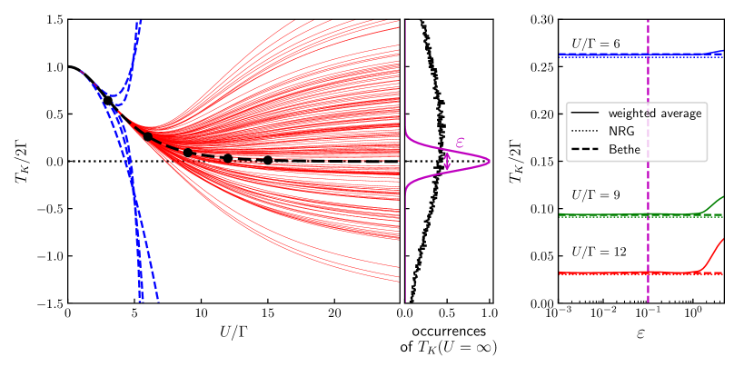
Figure 6: Reduction of the statistical noise on the resummed $T_{K}(U)$ series by Bayesian inference. Left panel: Kondo temperature as a function of $U$. The bundle of red lines correspond to different samples of our series after resummation (see text). The thick line shows the final result after Bayesian inference while the circles show our reference NRG calculations. The dashed blue lines show the bare results without resummation, which diverge for $U>5\Gamma$. Middle panel: histogram of the values of $T_{K}(U=\infty)$ obtained from our samples (black line), histogram of its assumed distribution with tolerance $\varepsilon$ (purple line). Right panel: final result after inference as a function of $\varepsilon$ for three values of $U/\Gamma=6,9$ and $12$ (thin lines), reference NRG result (dotted lines), Bethe ansatz result (dashed horizontal lines).

III.2.3 Noise reduction with Bayesian inference

Let us now apply the Bayesian inference technique described above to the computation of $T_{K}(U)$. In the left panel of Fig. 6 we have re-sampled the series for the Kondo temperature, i.e. we have generated many series (typically $10^{3}$ to $10^{5}$ samples). For each sample we perform the conformal transformation and plot the result for the Kondo temperature as a function of $U$ (thin red lines). While we find that all results agree for $U\leq 6\Gamma$, the bundle of curves start to diverge for larger values of $U$. In the middle panel, we plot (black thin line) the corresponding histogram of the values obtained for $T_{K}(U=\infty)$, which is $P_{\rm prior}(T_{K}=g(f))$.

We use the non-perturbative relation $\lim_{U\rightarrow\infty}T_{K}(U)=0$. Hence we want to “post-select” the configuration of $F_{n}$ which give a vanishing Kondo temperature at large $U$, at precision $\epsilon$. Following the procedure described in Sec. III.1.3, our final result is obtained by averaging the different traces (thin red lines) with the weight given by Eq. (14). The right panel of Fig. 6 shows the result for three different values of $U$ as a function of $\varepsilon$ which confirms that the results are insensitive to the actual value of $\varepsilon$. We find a very good agreement with the results obtained from NRG even at large values of $U$, noting that NRG spectra have typical relative error bars of a few percents (see Sec. IV.1 for details).

III.2.4 Benchmark with the Bethe Ansatz exact solution

The series expansion for $1/T_{K}(U)$ has been calculated explicitly and exactly using the Bethe Ansatz technique by Horvatic and ZlaticHorvatić, B. and Zlatić, V. (1985). Ref.Horvatić, B. and Zlatić, V., 1985 provides an iterative formula for calculating the coefficients of the expansions and shows that the corresponding series has an infinite radius of convergence. This provide another independent benchmark of the calculation of $T_{K}(U)$ as well as of the method itself. We checked that the 10 first coefficients of this series agree with the one that we computed with QMC.

Fig. 3 shows our final result together with the NRG result (black circles) and the Bethe ansatz results. At this scale, the agreement is perfect. Using the exact series for $1/T_{K}(U)$ (truncated to around 50 coefficients), we studied its zeros which are the poles of $T_{K}(U)$. We find that they are situated on the imaginary axis. The poles closest to the origin are $U/\Gamma\approx\pm 4.89059579i$ in agreement with our findings, see Fig. 4. The next poles are $U/\Gamma\approx\pm 13.79i$, $21.77i$, $29.89i$, $37.87i$ and $45.9i$ but are too far to be accessible with only the first ten coefficients. The right panel of Fig.6 provides a detailed benchmark of our results versus both NRG and the exact Bethe Ansatz solution.

We find that the QMC results for $T_{K}$ are slightly more accurate than NRG, because the extraction of $T_{K}$ from the NRG self-energy (see Eq. (15)) contains inherent broadening errors. The agreement between all three methods is nevertheless excellent. In addition, we can extract from the Bethe Ansatz the exact QMC error, and this error matches the measured 1 sigma statistical error bars.

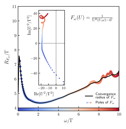
Figure 7: Main frame: convergence radius $R_{F_{\omega}}$ of $F_{\omega}(U)=1/(\Sigma^{R}(U,\omega)-i\Gamma)$ (thin line) in the equilibrium symmetric Anderson impurity model. The color circles show the absolute value of the pole of $F_{\omega}(U)$. Inset: position of the pole of $F_{\omega}(U)$ in the $U^{2}$ complex plane for different frequencies. The color blue to red corresponds to increasing frequency, as in the main frame. At high frequency, the statistical uncertainty prevents an accurate localization of the poles.

III.3 Equilibrium dynamical correlation functions

Let us now apply our method to the Green’s function and self-energy as a function of the real frequency $\omega$.

III.3.1 Singularities in the long time (stationary) limit

Let us now turn to the full Green’s function $G^{R}(\omega,U)$ and self-energy $\Sigma^{R}(\omega,U)$. An example of our bare data is shown in Fig. 2 where we plot the coefficients $\Sigma_{n}^{R}(\omega)$ obtained from real time diagrammatic quantum Monte-Carlo for $n=2,4,6,8$ and $10$. The description of the method used to calculate these coefficients $\Sigma_{n}^{R}(\omega)$ is explained in the companion paper to this articleBertrand et al. (2019).

We focus on the quantity $\Sigma^{R}(\omega)-i\Gamma$ and denote its inverse $F_{\omega}(U)=1/(\Sigma^{R}(\omega)-i\Gamma)$. The retarded Green’s function can be recovered from $F_{\omega}(U)$ using $G^{R}(\omega)=1/(\omega-F_{\omega}(U)^{-1})$ (using $\omega-\Sigma^{R}(\omega)+i\Gamma$ turns out to be less convenient especially at high frequency).

Fig. 7 shows the convergence radius of $F_{\omega}(U)$ as a function of frequency, extracted from a study of the exponential decay of the corresponding series with $n$. We have also performed a systematic study of the zeros of $\Sigma^{R}(\omega)-i\Gamma$ in order to localize the poles of $F_{\omega}(U)$. We find one pair of poles at each frequency. The results are shown in the inset of Fig. 7 for a set of frequencies from $\omega=0$ to $\omega=10\Gamma$ in the complex plane for $U^{2}$. The absolute value of the poles of $F_{\omega}(U)$ is also plotted in the main frame of Fig. 7 as a function of frequency (circles of varying colors from blue to red). We observe a perfect match with our estimation of the convergence radius reflecting the fact that these poles are responsible for the divergence of the series. It is important to note here that working in the real frequency domain is very helpful: we found a single pole per frequency (at least for the range of interactions that we could study). Hence, we expect that performing the resummation in real time or imaginary frequencies could be more complex, since all these poles would be involved simultaneously.

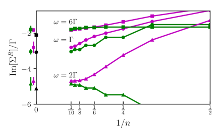
Figure 8: Resummation of the self-energy in the equilibrium symmetric Anderson impurity model at $U=9\Gamma$. The imaginary part of $\Sigma^{R}(\omega)$ is shown as a function of the number $n$ of terms kept in the resummation, for three frequencies $\omega=\Gamma$ (circles), $2\Gamma$ (triangles) and $6\Gamma$ (squares). The independent resummation of $F_{\omega}(U)$ (green line) and of $\Sigma^{R}(\omega)-i\Gamma$ (purple line) converge with one another. The results with truncation and statistical errors are shown on the left of the y-axis, along with NRG results (black symbols).

The results for three frequencies ($\omega/\Gamma=1,2$ and $6$) are given in Fig. 8. We show the convergence of the imaginary part of the self-energy using two different resummed series: $F_{\omega}(U)$ (green symbols) and $1/F_{\omega}(U)$ (purple symbols). The former has been resummed with an Euler transform with a frequency dependant $p$ set close to the poles shown in Fig. 7. The latter, for which our method did not detect poles, has been resummed with the parabola transform (in the $U$ plane) with $p=-4.5\Gamma$. Again, Bayesian inference has been used to enforce $\lim_{U\rightarrow\infty}G(U,\omega)=0$ for all $\omega\neq 0$. For comparison, we also include the NRG results (which are very accurate at small frequency and possibly less accurate at large frequency). The slight difference between the purple and green curves is due to the truncation error. We find that the series which has (initially) the largest convergence radius is less sensitive to truncation error or statistical noise than the other. We attribute the small discrepancy between the QMC results and NRG at large frequency to a lack of convergence of the latter. These results are obtained for a rather strong interaction $U=9\Gamma$. At smaller interaction the QMC and NRG results become undistinguishable. At larger interactions, the QMC results become increasingly inaccurate due to truncation errors.

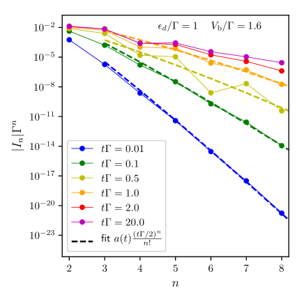
Figure 9: Coefficients (absolute value) of the series for the current (circles with thin lines) in the asymmetric model ($\varepsilon_{d}=\Gamma$, $V_{\rm b}=1.6\Gamma$) computed at different times $t$ (different colors). The apparent convergence radius decreases with time. For small values of $t$, we can observe that the series coefficients decrease faster than exponentially, which indicates an infinite convergence radius. The thick dashed line shows the corresponding fit with $(t\Gamma/2)^{n}/n!$. For large enough $t$, the series converges toward the steady state limit.

III.3.2 The long time limit

In the Keldysh formalism, the interactions are switched on at an initial time (0), and one follows the evolution of the system with time $t$. We assume here that the system relaxes to a steady state at long time. Let us consider the average of an operator ${\cal\hat{O}}$ as a function of time, and its expansion $\langle{\cal\hat{O}}(t)\rangle=\sum_{n}O_{n}(t)U^{n}$ (the extension of the following arguments to Green’s function is straightforward).

At finite time $t$, the radius of convergence of this series is infinite, as shown in Appendix B. Each order in the perturbation expansion $O_{n}(t)$ relaxes with $t$ to a long time limit, but the time $t_{\text{relax}}(n)$ it takes to reach this limit can increase with $n$. The long time and large $n$ limit do not commute in general:

$$\lim_{n\rightarrow\infty}\lim_{t\rightarrow\infty}O_{n}(t)\neq\lim_{t\rightarrow\infty}\lim_{n\rightarrow\infty}O_{n}(t).$$ (18)

This behaviour was already noted in Fig. 14 of Ref. Profumo et al., 2015. It is also illustrated on Fig. 9, which shows various orders $n$ of the expansion of the current through the dot versus $n$, for different times. We observe that at small times the orders $I_{n}$ decreases faster than exponentially with $n$, consistent with the bound mentioned above. The coefficients converge to the steady state limit at long time.

At finite time $t$, since the series converges, it is sufficient to have enough orders. In the steady state, as explained above, we have a minimal order $N_{0}$ needed to compute the quantity at a given precision. One should then simply compute at a time $t>t_{\text{relax}}(N_{0})$.

In the Anderson model, some quantities like the spectral function are known to relax on a long time scale $t_{K}\sim T_{K}^{-1}$, see e.g. Ref. Nordlander et al., 1999. The previous remarks explain how the algorithm deals with this long time. For a given $U$, we need $N_{0}(U)$ orders, hence to compute at a time larger than $t_{\text{relax}}(N_{0}(U))$. The larger $U$ is, the longer this time becomes. However, it is still finite at fixed $U$, and since our calculation of the perturbative expansion is uniform in time, it is not an issue (the computation effort does not grow with time). However, the existence of the Kondo time indicates that the number of orders necessary to compute e.g. the low frequency spectral function at a given $U$ increases with $U$ (otherwise the relaxation time of the physical quantity would be bounded at large $U$).

IV Benchmark of the dynamics in equilibrium

We now benchmark our results in the case of equilibrium, testing various regimes of the Anderson impurity model. Let us first describe the high-precision NRG computations that were performed.

IV.1 NRG implementation

The Numerical Renormalization Group (NRG) Bulla et al. (2008) was used to benchmark our QMC calculations in equilibrium, and to test the reliability of the series extrapolation method for spectral functions at various values of $U$ and $\epsilon_{d}$. In order to obtain precise NRG data for the spectral function of the Anderson impurity model, the computations were performed using several improvements over the simplest implementations of the NRG. First, the full density matrix formulation of NRG Hofstetter (2000) was used to reduce finite size effects due to the NRG truncation. Second, symmetries of the problem were heavily exploited Tóth et al. (2008), allowing to reduce significantly the Hilbert space dimension of various multiplets. In the particle-hole symmetric case, the full SU(2)${}_{\mathrm{charge}}\otimes$SU(2)_spin symmetry was used, while the charge sector was reduced to U(1)_charge away from particle-hole symmetry. Third, the impurity Green’s function was extracted from a direct computation of the $d$-level self-energy $\Sigma(\omega)$ Bulla et al. (1998), according to its exact representation as the ratio of two retarded correlation functions in the frequency domain:

$$\Sigma(\omega)=U\frac{F^{R}(\omega)}{G^{R}(\omega)},$$ (19)

where $G^{R}(t)=-i\theta(t)\langle\{d^{\phantom{\dagger}}_{\sigma}(0),d_{\sigma}^{\dagger}(t)\}\rangle$ is the usual single particle retarded Green’s function in the time domain, and $F^{R}(t)=-i\theta(t)\langle\{d^{\phantom{\dagger}}_{\sigma}(0)d_{-\sigma}^{\dagger}(0)d^{\phantom{\dagger}}_{-\sigma}(0),d_{\sigma}^{\dagger}(t)\}\rangle$ is a composite fermionic correlation function. In practice, $\mathrm{Im}[G^{R}(\omega)]$ and $\mathrm{Im}[F^{R}(\omega)]$ are computed from the Källén-Lehmann representation using the broadened NRG spectra, and the real parts of both $G^{R}(\omega)$ and $F^{R}(\omega)$ are obtained via a Kramers-Kronig relation. Finally, the truncation parameters of the NRG simulations were taken to model as closely as possible a continuous density of states for the electronic bath. Although the use of the logarithmic Wilson discretization grid, $\omega_{n}=D\Lambda^{-n}$, is inherent to the practical success of NRG, we found that values of $\Lambda$ as low $\Lambda=1.4$ could be managed in practice within the NRG, taking a very large number $N_{\mathrm{kept}}=3200$ of kept multiplets. Up to $N_{\mathrm{iter}}=120$ NRG iterations were used, so that the effective temperature can be considered to be practically zero. With such small value of $\Lambda$, the broadening parameter $b$ of the discrete NRG spectra could be decreased down to $b=0.2$, without $z$-averaging, which further enhanced the spectral resolution of the Hubbard satellites in the spectral function.

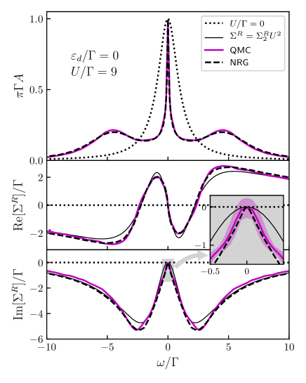
Figure 10: Resummed equilibrium spectral function (upper panel), real part (middle panel) and imaginary part (lower panel) of the retarded self energy $\Sigma^{R}(\omega)$ for the symmetric Anderson impurity $\epsilon_{d}/\Gamma=0$ at $U=9\Gamma$. Purple line: resummed result from $10$ orders of perturbation theory; dashed line: NRG; dotted line: non-interacting result; thin black line: second order perturbation theory for the self-energy. Inset: zoom of the imaginary part at small energy with error bars.

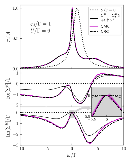
Figure 11: Resummed equilibrium spectral function (upper panel), real part (middle panel) and imaginary part (lower panel) of the retarded self energy $\Sigma^{R}(\omega)$ for the asymmetric Anderson impurity $\epsilon_{d}/\Gamma=1$ at $U=6\Gamma$. Purple line: resummed result from $10$ orders of perturbation theory; dashed line: NRG; dotted line: non-interacting result; thin black line: second order perturbation theory for the self-energy. Inset: zoom of the imaginary part at small energy with error bars.

IV.2 Comparison to NRG in equilibrium

Fig. 10 shows the spectral function as well as the imaginary and real part of the self energy for the symmetric Anderson impurity in the strong correlation regime $U=9\Gamma$ (same data as the purple curve of Fig. 8). The spectral function shows a clear Kondo peak and the two satellites at $\omega\simeq\pm 4.5\Gamma=\pm U/2$ in good agreement with the NRG data. For this calculation, a simple second order calculation of the self-energy already provides a reasonably good result (thin black line), due to near cancellations in higher order diagrams in the peculiar case of particle-hole symmetry.

Fig. 11 shows the same plot in the asymmetric case $\epsilon_{d}=1$. This case is more complex because the resonance at $U=0$ is offset with respect to the Fermi level, hence to the position of the Kondo peak. We note that previous real time QMC techniques suffered from a strong sign problem and could not access the asymmetric regime Werner et al. (2010). We also stress that the second order approximation is now very different from the correct result. The comparison to the NRG data is still excellent.

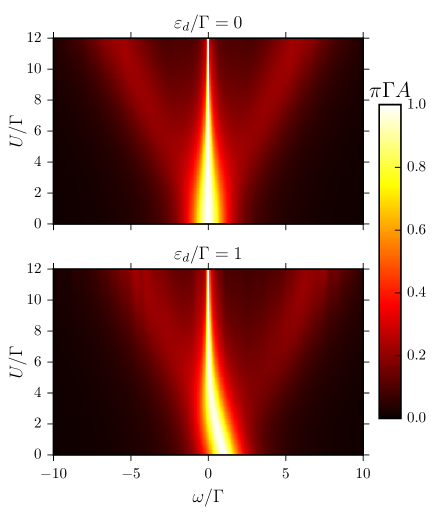
Figure 12: Color plot of the spectral density $A(\omega,U)$ in the symmetric case ($\epsilon_{d}/\Gamma=0$, upper panel) and asymmetric case ($\epsilon_{d}/\Gamma=1$, lower panel) as a function of $\omega$ and $U$. The data from each panel has been obtained in a single QMC run.

Another advantage of the techniques described in this article and its companion article Bertrand et al. (2019) is that a single QMC run provides the full dependence in both $\omega$ and $U$, which is very time consuming in the NRG. This is illustrated in Fig. 12 where the color map shows the spectral function as a function of $\omega$ and $U$. One can clearly observe the formation of the Kondo peak (which gets thinner as one increases $U$ and shifts toward $\omega=0$ in the asymmetric case) as well as the Hubbard bands at $\omega=\pm U/2$. Note that the results are perfectly well behaved (qualitatively correct) up to very large $U$ (even above $U=12\Gamma$ shown in the plot) but become quantitatively inaccurate at too large values of $U$. Improving them would require the use of higher perturbation orders.

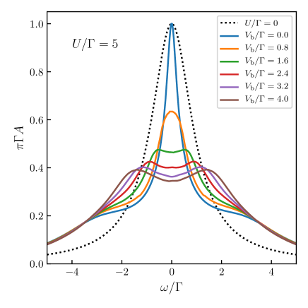
Figure 13: Out-of-equilibrium spectral functions with interaction strength $U/\Gamma=5$, in the symmetric ($\epsilon_{d}/\Gamma=0$) model with a symmetric voltage bias $V_{\rm b}$. The resulting self-energy series has been resummed in a similar fashion as for the previous results. The non-interacting spectral function is shown as a dotted line.

V Out of equilibrium results

We finally turn to the out-of-equilibrium regime, and present some accurate computation of current-voltage characteristics, as well as novel predictions for dynamical observables in presence of a finite bias voltage.

V.1 Splitting of the spectral function

Fig. 13 shows the spectral function of the symmetric impurity in the presence of various bias voltages from $V_{\rm b}=0$ to $4\Gamma$. The results were obtained using the parabolic map on the series of $\Sigma_{\omega}(U^{2})-i\Gamma$ (with an optimized frequency dependent parameter $p/\Gamma^{2}\in[-25,-200]$). Upon increasing the bias voltage, we find as expected from NCAWingreen and Meir (1994) and perturbativeFujii and Ueda (2003) calculations that the Kondo resonance simultaneously broadens and get split into two peaks. Previous results on the spectral functionCohen et al. (2014b) were based on the bold diagrammatic approach and were calculated at relatively high temperature ($T=\Gamma/3$) while using a third terminal for computing the spectral function.

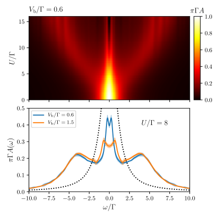
Figure 14: Out-of-equilibrium spectral functions of the impurity with same parameters as in Fig. 13, except for temperature $T=\Gamma/50$. Upper panel: color plot of the spectral density as a function of $\omega$ and $U$ for a voltage bias $V_{\rm b}=0.6\Gamma$. Lower panel: spectral density at $U=8\Gamma$ for a bias $V_{\rm b}=0.6\Gamma$ (blue line) and $V_{\rm b}=1.5\Gamma$ (orange line). Error bars are shown as shaded areas. The dotted line shows the non-interacting density. No Bayesian inference has been used. Integration time is $20/\Gamma$.

Most of the results of this paper have been obtained at very low temperature. We emphasize however that increasing the temperature makes the calculations easier: indeed at finite temperature, the non-interacting Green’s functions decrease exponentially as $e^{-t/T}$ instead of the algebric decay at zero temperature. It follows that the support of the integrals to be calculated is smaller, hence the convergence of the calculation faster. We show a calculation at finite temperature in Fig. 14 where we have computed the spectral density of the symmetric impurity at temperature $T=\Gamma/50$ under a bias voltage $V_{\rm b}=0.6\Gamma$ and $V_{\rm b}=1.5\Gamma$. A single Monte-Carlo run allows us to observe the splitting of the Kondo resonance as $U$ is increased (upper panel). The result is quantitatively accurate up to $U\approx 8\Gamma$ (lower panel) but remains qualitatively meaningful at higher interaction (upper panel).

The fate of the Kondo resonance out-of-equilibrium, in presence of a bias voltage, can be understood qualitatively from the interplay of two phenomena. On the one hand, the bias voltage induces a splitting of the Fermi energies of the two reservoirs, hence one expects a corresponding splitting of the Kondo resonance. On the other hand, the voltage, like the temperature, increases the energy and phase space for the spin fluctuations, leading eventually to the disappearance of the Kondo resonanceHershfield et al. (1991, 1992); Anders (2008). The competition between both effects leads to the appearance of the splitting only above a finite voltage threshold (about $V_{b}\simeq\Gamma$ in the plot of Fig. 13).

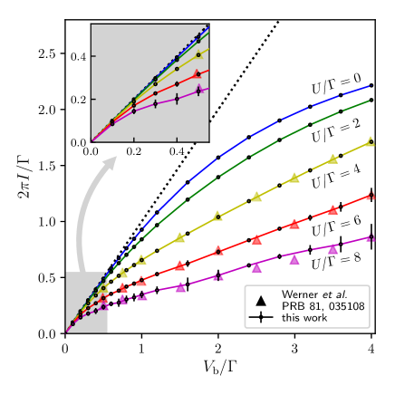
Figure 15: Current-voltage characteristics at different interaction strengths in the symmetric case $\epsilon_{d}=0$. Perturbation series for the current have been computed using the Landauer formula Eq. (7), then resummed. The results are consistent with a weak-coupling Quantum Monte-Carlo calculation from Werner et al.Werner et al. (2010) (triangles), but extends further down in bias.

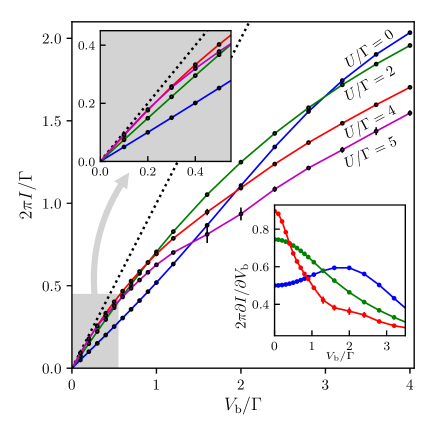
Figure 16: Current-voltage characteristics at different interaction strengths in the asymmetric model ($\epsilon_{d}/\Gamma=1$). The bottom-right inset shows the development of the zero-bias anomaly in the differential conductance when $U$ increases ($U/\Gamma=0$ in blue, $2$ in green and $4$ in red).

V.2 I-V transport characteristics

Fig. 15 shows the results obtained for the I-V characteristics in the symmetric case $\epsilon_{d}=0$. The resummation has been done for the series of $1/I(U^{2})$ using a parabolic transform with $p=-40\Gamma^{2}$. At small bias, we recover a perfect transmission $I=(e^{2}/h)V_{\rm b}$ due to the unitary Kondo resonance, while for $eV_{\rm b}>k_{B}T_{K}$ the conductance experiences an extra suppression by the interaction (Coulomb blockade). We find a very good match with a previous calculation from Ref. Werner et al., 2010. The present technique allows one to lift the main limitations that Ref. Werner et al., 2009, 2010 was facing: we can now access long times (here we have used $\sim 20/\Gamma$ but it could be increased further if necessary) to be compared with maximum times of the order of $\sim 3-5/\Gamma$ in Ref. Werner et al., 2010. As a consequence, we can reach the low bias regime, which was not accessible in Ref. Werner et al., 2010. Another important point is that the method is not limited to the symmetry point as we now demonstrate.

Fig. 16 shows the $I-V$ characteristics for an asymmetric model with $\epsilon_{d}/\Gamma=1$. The results have been obtained from the resummation of $1/I(U)$ with a parabolic transform ($p=-6\Gamma$) and no Bayesian inference. The $I-V$ characteristics is particularly interesting because, due to the asymmetry, the non-interacting low bias transmission is modified by interactions and one must first build up the Kondo resonance to approach $I\simeq(e^{2}/h)V_{\rm b}$ (note that the unitary limit is strictly exact only at $\epsilon_{d}=0$, and the conductance is slightly lower than $e^{2}/h$ otherwise in the Kondo regime). This behavior leads to a non monotonous current versus $U$: as one increases $U$, the current first increases until the Kondo resonance is fully built (see the bottom panel of Fig. 12). As one increases further $U$, the Kondo width $T_{K}$ shrinks and the current decreases as Coulomb blockade starts to set in.

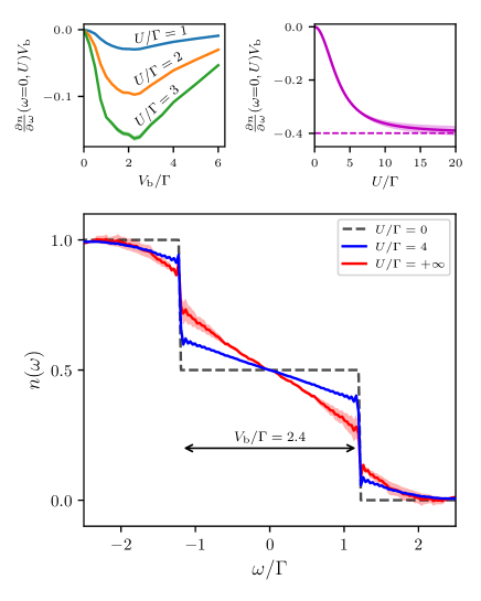
Figure 17: Lower panel: out-of-equilibrium electron distribution function on the impurity ($\epsilon_{d}/\Gamma=0$) under a bias voltage $V_{\rm b}=2.4\Gamma$. The distribution function is defined as in Eq. (20). Increasing the interaction strength ($U/\Gamma=4$ blue line, $U/\Gamma=+\infty$ red line) leads to a softening of the characteristic double-step of the non-interacting distribution function (dashed line). It is linear between the Fermi levels of the two leads. The Euler transform has been used for resummation and the result has not been submitted to Bayesian inference. Upper panels: normalized slope of the distribution function near $\omega=0$ as a function of bias voltage (left panel) and interaction strength (right panel). For intermediate interaction, the normalized slope reaches an extremum near $V_{\rm b}=2\Gamma$ (left panel). At strong interaction, the normalized slope saturates (right panel, for $V_{\rm b}=2.4\Gamma$).

V.3 Biased distribution function

Finally, we discuss the out-of-equilibrium distribution function of the impurity, i.e. its energy-dependent probability of occupation. We define the distribution function $n(\omega)$ as

$$n(\omega)=\frac{G^{<}(\omega)}{2\pi iA(\omega)},$$ (20)

so that at equilibrium $n(\omega)$ is simply the Fermi function $n_{F}(\omega)$. Without interaction, the distribution function amounts (at zero temperature) to a double step function $n(\omega)_{U=0}=[n_{F}(\omega-V_{\rm b}/2)+n_{F}(\omega+V_{\rm b}/2)]/2$. We want to investigate the behaviour of $n(\omega)$ as $U$ increases, a question that was not addressed in previous literature to the best of our knowledge.

The results are shown in Fig. 17. In this particular case, the series are fully alternated which means that the singularity lies on the negative real axis. We could sum the series using an Euler transform ($p=-8\Gamma^{2}$) up to $U=+\infty$. We find that the function $n(\omega)$ is not thermal, i.e. it can not be fitted by a Fermi function $n_{F}$ with an effective temperature. In particular, it still exhibits discontinuities at the position of the lead Fermi surfaces, which we expect to be rounded at finite temperature. Interestingly, these discontinuities are comparable to the equilibrium quasiparticle weight for $U=4\Gamma$, do not seem to vanish in the limit $U=\infty$. Also very striking is the quasi-linear behavior of $n(\omega)$ that is observed for $-V_{b}/2<\omega<V_{b}/2$.

Experiments that measure the non-equilibrium distribution function quantity typically use a third (for instance superconducting) terminal weakly coupled to the system Pothier et al. (1997); Anthore et al. (2003); Huard et al. (2004); Chen et al. (2009). To the best of our knowledge, this quantity has not been measured in quantum dots, and we hope that the present prediction may stimulate some experimental activity.

VI Conclusion: The fall of the convergence wall

We have presented a systematic computation of the perturbative expansion of the Anderson impurity model in and out of equilibrium in power of the interaction strength $U$. The main advantage of our Keldysh expansion approach is its ability to calculate directly in the long time steady state regime. Using our approach, we were able to obtain improved or novel results regarding the non-equilibrium dynamics of strongly interacting quantum dots.

The main contribution of this article lies in the systematic construction of a set of conformal transformations that provide a practical route for a mathematically controlled resummation of series. We have shown how to use analytic conformal transform guided by an approximated location of the singularities of the physical quantities in the $U$ complex plane. We also presented a Bayesian method to control the strong amplification of statistical noise during this procedure, using some simple non-perturbative information. The combination of singularity location, conformal transform crafting and Bayesian inference provides a robust and generic resummation methodology.

It was noticed recentlyRossi, R. et al. (2017) that for values of $U$ inside the convergence radius, connected diagrammatic quantum Monte-Carlo techniques provide a systematic route for calculating the many-body quantum problem in a computational time that only increases polynomially with the requested precision. We argue that the argument of Ref. Rossi, R. et al., 2017 can be directly extended to systems where the separation hypothesis holds (switching from working with the series in $U$ to the series in $W$). We conclude that, in general, systems where the separation hypothesis hold can be computed with a computing time that increases polynomially with the requested precision.

The approach presented here may have implications for a large class of other problems within or beyond condensed matter physics. In particular, a possible extension is to build a real time (equilibrium or non-equilibrium) quantum impurity solver for DMFT or its extensions, or directly addressing lattice problems such as the Hubbard model. At its core, it consists in techniques to efficiently compute the bare perturbation series and to sum it. Its limitations remain to be explored. They could come from a resurgence of the sign problem, which would manifest itself in a very oscillatory nature of the integrals for expansion coefficients, making them hard to evaluate, or from a difficulty to sum the perturbative series, in particular for systems with a phase transition, or a non-Fermi liquid fixed point at low temperature. In order to address these questions, the technique needs to be applied to more complex models. Work is in progress in this direction.

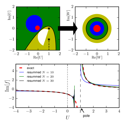
Figure 18: Resummation of the series of $f(U)=1/\ln(i(1-U)+1)$ near $U=0$ on the real positive axis, beyond the pole at $U=1$. $f$ has a pole at $U=1$ and a branch cut starting at $U=1-i$ and going in straight line toward $1-i\infty$ (stars and dashed line in upper left panel). We isolated these singularities by applying a conformal map $W=\frac{\chi(U)-\chi(0)}{\chi(U)-\chi(0)^{*}}$, with $\chi(U)=i\sqrt{(U-1)/p}-i$. It maps the inside of a parabola into the outside of the unit disk (left and right upper panels). $p$ controls the direction and width of the parabola. Here $p=0.2e^{i\pi\times 0.4}$. With $N=30$ terms, one can compute $f$ for all real $U$ (black plain line) except a narrow band around the pole (dashed black vertical line).

Appendix A A toy model function with a singularity on the real axis

We present here on Fig. 18 a toy model for the resummation of a function $f(U)=1/\ln(i(1-U)+1)$ that has a pole on the real axis at $U=1$ as well as a branch cut on the curve $U=1-i(1+x)$ with $x\in[0,\infty]$. The aim of this toy model is to show that even though $f(U)$ has a singularity on the real axis (and hence it will be difficult to calculate close to this singularity), it is possible to calculate the function beyond the singularity using a conformal transformation. We use the conformal map $W=\frac{\chi(U)-\chi(0)}{\chi(U)-\chi(0)^{*}}$, with $\chi(U)=i\sqrt{(U-1)/p}-i$ that maps the inside of a parabola into the outside of the unit disk (see the upper left and right panels of Fig. 18). The lower panel of Fig. 18 shows the corresponding resummed series using $N=10,20$ and $30$ terms in the expansion of $f(U)$. Although we cannot calculate close to $U=1$, we find that with as little as $N=20$ terms in the expansion of $f(U)$, we can recover an accurate description of $f(U)$ for $U>1.2$ from an expansion around $U=0$.

Appendix B Convergence of the perturbation series at finite time

In this appendix, we show that at finite time $t$, the radius of convergence of the perturbation series for an operator $\cal{O}$ is infinite, for a system with an interaction on a finite number of sites and an infinite bath. Indeed, the average is given by

$$\langle{\cal\hat{O}}(t)\rangle\propto\left\langle T_{c}e^{-iU\int du\hat{\mathrm{{\textbf{H}}}}_{\rm int}(u)}{\cal\hat{O}}(t)\right\rangle,$$ (21)

where the integral goes along the forward-backward Keldysh contour $0\rightarrow t\rightarrow 0$, the operators are taken in the interaction representation, $T_{c}$ is the usual Keldysh contour ordering operator and $\hat{\mathrm{{\textbf{H}}}}_{\rm int}(u)$ is the interacting part of the Hamiltonian.

More precisely, each of the $2^{n}$ terms of the expansion of the exponential has the form,

$$\frac{U^{n}}{n!}\int_{[0,t]^{n}}du_{1}...du_{n}\langle{\cal\hat{O}}(t)C(u_{1},\ldots u_{n})\rangle.$$

where $C$ is a product of $c$, $c^{\dagger}$, and unitary time evolution operators. The terms $\langle{\cal\hat{O}}(t)C(u_{1},\ldots u_{n})\rangle$ are amplitudes of probability for quantum processes and are therefore bounded. Explicitly,

$$\langle{\cal\hat{O}}(t)C(u_{1},\ldots u_{n})\rangle =\mathrm{Tr}\left(\frac{e^{-\beta H_{0}}}{Z_{0}}{\cal\hat{O}}(t)C(u_{1},\ldots u_{n})\right)$$

$$=\sum_{\psi}\langle\psi|\frac{e^{-\beta H_{0}}}{Z_{0}}{\cal\hat{O}}(t)C(u_{1},\ldots u_{n})|\psi\rangle$$

$$\left|\langle{\cal\hat{O}}(t)C(u_{1},\ldots u_{n})\rangle\right| \leq\sum_{\psi}\frac{e^{-\beta H_{0}}}{Z_{0}}\mathinner{\!\left\lVert{\cal\hat{O}}(t)C(u_{1},\ldots u_{n})\psi\right\rVert}$$

$$\leq\sum_{\psi}\frac{e^{-\beta H_{0}}}{Z_{0}}\mathinner{\!\left\lVert{\cal\hat{O}}(t)C(u_{1},\ldots u_{n})\right\rVert}\mathinner{\!\left\lVert\psi\right\rVert}$$

$$\leq\mathinner{\!\left\lVert{\cal\hat{O}}\right\rVert},$$

where $\mathinner{\!\left\lVert v\right\rVert}$ is the norm for a vector and the induced norm for an operator. We note that the norm is not modified by the unitary evolution $\mathinner{\!\left\lVert e^{iH_{0}u}Ae^{-iH_{0}u}\right\rVert}=\mathinner{\!\left\lVert A\right\rVert}$ for any operator $A$, and for the canonical operators $\mathinner{\!\left\lVert c\right\rVert}=1$, as can be checked in the Fock basis, independently of the size of the bath. Since the norm is sub-multiplicative, we obtain the last inequality.

Therefore, the term of order $n$ in the expansion of (21) is controlled by a bound $\frac{\mathinner{\!\left\lVert{\cal O}\right\rVert}(2UtL)^{n}}{n!}$, so the series has an infinite radius of convergence. Note that this argument is valid because the electron-electron interaction is present on a finite number of sites only. It would not apply directly to e.g. the Hubbard model in the thermodynamic limit.

References

- Först et al. (2011) M. Först, C. Manzoni, S. Kaiser, Y. Tomioka, Y. Tokura, R. Merlin, and A. Cavalleri, Nature Physics 7, 854 (2011), eprint 1101.1878.
- Fausti et al. (2011) D. Fausti, R. I. Tobey, N. Dean, S. Kaiser, A. Dienst, M. C. Hoffmann, S. Pyon, T. Takayama, H. Takagi, and A. Cavalleri, Science 331, 189 (2011), ISSN 0036-8075, URL http://science.sciencemag.org/content/331/6014/189.
- Nicoletti et al. (2014) D. Nicoletti, E. Casandruc, Y. Laplace, V. Khanna, C. R. Hunt, S. Kaiser, S. S. Dhesi, G. D. Gu, J. P. Hill, and A. Cavalleri, Phys. Rev. B 90, 100503 (2014), URL https://link.aps.org/doi/10.1103/PhysRevB.90.100503.
- Casandruc et al. (2015) E. Casandruc, D. Nicoletti, S. Rajasekaran, Y. Laplace, V. Khanna, G. D. Gu, J. P. Hill, and A. Cavalleri, Phys. Rev. B 91, 174502 (2015), URL https://link.aps.org/doi/10.1103/PhysRevB.91.174502.
- Nicoletti and Cavalleri (2016) D. Nicoletti and A. Cavalleri, Adv. Opt. Photon. 8, 401 (2016), URL http://aop.osa.org/abstract.cfm?URI=aop-8-3-401.
- Nicoletti et al. (2018) D. Nicoletti, D. Fu, O. Mehio, S. Moore, A. S. Disa, G. D. Gu, and A. Cavalleri, Phys. Rev. Lett. 121, 267003 (2018), URL https://link.aps.org/doi/10.1103/PhysRevLett.121.267003.
- Nakamura et al. (2013) F. Nakamura, M. Sakaki, Y. Yamanaka, S. Tamaru, T. Suzuki, and Y. Maeno, Scientific Reports 3, 2536 EP (2013), article, URL https://doi.org/10.1038/srep02536.
- del Valle et al. (2018) J. del Valle, J. G. Ramírez, M. J. Rozenberg, and I. K. Schuller, Journal of Applied Physics 124, 211101 (2018), eprint https://doi.org/10.1063/1.5047800, URL https://doi.org/10.1063/1.5047800.
- Roch et al. (2009) N. Roch, S. Florens, T. A. Costi, W. Wernsdorfer, and F. Balestro, Phys. Rev. Lett. 103, 197202 (2009), URL https://link.aps.org/doi/10.1103/PhysRevLett.103.197202.
- Parks et al. (2010) J. J. Parks, A. R. Champagne, T. A. Costi, W. W. Shum, A. N. Pasupathy, E. Neuscamman, S. Flores-Torres, P. S. Cornaglia, A. A. Aligia, C. A. Balseiro, et al., Science 328, 1370 (2010), ISSN 0036-8075, URL http://science.sciencemag.org/content/328/5984/1370.
- Iftikhar et al. (2015) Z. Iftikhar, S. Jezouin, A. Anthore, U. Gennser, F. D. Parmentier, A. Cavanna, and F. Pierre, Nature 526, 233 EP (2015), URL https://doi.org/10.1038/nature15384.
- Iftikhar et al. (2018) Z. Iftikhar, A. Anthore, A. K. Mitchell, F. D. Parmentier, U. Gennser, A. Ouerghi, A. Cavanna, C. Mora, P. Simon, and F. Pierre, Science 360, 1315 (2018), ISSN 0036-8075, URL http://science.sciencemag.org/content/360/6395/1315.
- Giamarchi (2004) T. Giamarchi, Quantum physics in one dimension, Internat. Ser. Mono. Phys. (Clarendon Press, Oxford, 2004), URL http://cds.cern.ch/record/743140.
- Thomas et al. (1996) K. J. Thomas, J. T. Nicholls, M. Y. Simmons, M. Pepper, D. R. Mace, and D. A. Ritchie, Phys. Rev. Lett. 77, 135 (1996), URL https://link.aps.org/doi/10.1103/PhysRevLett.77.135.
- Thomas et al. (1998) K. J. Thomas, J. T. Nicholls, N. J. Appleyard, M. Y. Simmons, M. Pepper, D. R. Mace, W. R. Tribe, and D. A. Ritchie, Phys. Rev. B 58, 4846 (1998), URL https://link.aps.org/doi/10.1103/PhysRevB.58.4846.
- Micolich (2011) A. P. Micolich, Journal of Physics: Condensed Matter 23, 443201 (2011), URL https://doi.org/10.1088%2F0953-8984%2F23%2F44%2F443201.
- Preskill (2018) J. Preskill, Quantum 2, 79 (2018), ISSN 2521-327X, URL https://doi.org/10.22331/q-2018-08-06-79.
- Reininghaus et al. (2014) F. Reininghaus, M. Pletyukhov, and H. Schoeller, Phys. Rev. B 90, 085121 (2014), URL https://link.aps.org/doi/10.1103/PhysRevB.90.085121.
- Schwarz et al. (2018) F. Schwarz, I. Weymann, J. von Delft, and A. Weichselbaum, Phys. Rev. Lett. 121, 137702 (2018), URL https://link.aps.org/doi/10.1103/PhysRevLett.121.137702.
- Fujii and Ueda (2003) T. Fujii and K. Ueda, Phys. Rev. B 68, 155310 (2003), URL https://link.aps.org/doi/10.1103/PhysRevB.68.155310.
- Van Roermund et al. (2010) R. Van Roermund, S.-y. Shiau, and M. Lavagna, Phys. Rev. B 81, 165115 (2010), URL https://link.aps.org/doi/10.1103/PhysRevB.81.165115.
- Wingreen and Meir (1994) N. S. Wingreen and Y. Meir, Phys. Rev. B 49, 11040 (1994), URL https://link.aps.org/doi/10.1103/PhysRevB.49.11040.
- White (1992) S. R. White, Phys. Rev. Lett. 69, 2863 (1992), URL https://link.aps.org/doi/10.1103/PhysRevLett.69.2863.
- White (1993) S. R. White, Phys. Rev. B 48, 10345 (1993), URL https://link.aps.org/doi/10.1103/PhysRevB.48.10345.
- Schollwöck (2005) U. Schollwöck, Rev. Mod. Phys. 77, 259 (2005), URL https://link.aps.org/doi/10.1103/RevModPhys.77.259.
- Anders and Schiller (2005) F. B. Anders and A. Schiller, Phys. Rev. Lett. 95, 196801 (2005), URL https://link.aps.org/doi/10.1103/PhysRevLett.95.196801.
- Heidrich-Meisner et al. (2009) F. Heidrich-Meisner, A. E. Feiguin, and E. Dagotto, Phys. Rev. B 79, 235336 (2009), URL https://link.aps.org/doi/10.1103/PhysRevB.79.235336.
- Eckel et al. (2010) J. Eckel, F. Heidrich-Meisner, S. G. Jakobs, M. Thorwart, M. Pletyukhov, and R. Egger, New Journal of Physics 12, 043042 (2010), URL https://doi.org/10.1088%2F1367-2630%2F12%2F4%2F043042.
- Mühlbacher and Rabani (2008) L. Mühlbacher and E. Rabani, Phys. Rev. Lett. 100, 176403 (2008), URL https://link.aps.org/doi/10.1103/PhysRevLett.100.176403.
- Werner et al. (2009) P. Werner, T. Oka, and A. J. Millis, Phys. Rev. B 79, 035320 (2009), URL https://link.aps.org/doi/10.1103/PhysRevB.79.035320.
- Werner et al. (2010) P. Werner, T. Oka, M. Eckstein, and A. J. Millis, Phys. Rev. B 81, 035108 (2010), URL https://link.aps.org/doi/10.1103/PhysRevB.81.035108.
- Schiró and Fabrizio (2009) M. Schiró and M. Fabrizio, Phys. Rev. B 79, 153302 (2009), URL https://link.aps.org/doi/10.1103/PhysRevB.79.153302.
- Schiró (2010) M. Schiró, Phys. Rev. B 81, 085126 (2010), URL https://link.aps.org/doi/10.1103/PhysRevB.81.085126.
- Cohen et al. (2014a) G. Cohen, D. R. Reichman, A. J. Millis, and E. Gull, Phys. Rev. B 89, 115139 (2014a), URL https://link.aps.org/doi/10.1103/PhysRevB.89.115139.
- Cohen et al. (2014b) G. Cohen, E. Gull, D. R. Reichman, and A. J. Millis, Phys. Rev. Lett. 112, 146802 (2014b), URL https://link.aps.org/doi/10.1103/PhysRevLett.112.146802.
- Cohen et al. (2015) G. Cohen, E. Gull, D. R. Reichman, and A. J. Millis, Phys. Rev. Lett. 115, 266802 (2015), URL https://link.aps.org/doi/10.1103/PhysRevLett.115.266802.
- Chen et al. (2017a) H.-T. Chen, G. Cohen, and D. R. Reichman, The Journal of Chemical Physics 146, 054105 (2017a), eprint https://doi.org/10.1063/1.4974328, URL https://doi.org/10.1063/1.4974328.
- Chen et al. (2017b) H.-T. Chen, G. Cohen, and D. R. Reichman, The Journal of Chemical Physics 146, 054106 (2017b), eprint https://doi.org/10.1063/1.4974329, URL https://doi.org/10.1063/1.4974329.
- Profumo et al. (2015) R. E. V. Profumo, C. Groth, L. Messio, O. Parcollet, and X. Waintal, Phys. Rev. B 91, 245154 (2015), URL https://link.aps.org/doi/10.1103/PhysRevB.91.245154.
- Georges et al. (1996) A. Georges, G. Kotliar, W. Krauth, and M. J. Rozenberg, Rev. Mod. Phys. 68, 13 (1996), URL https://link.aps.org/doi/10.1103/RevModPhys.68.13.
- Kotliar et al. (2006) G. Kotliar, S. Y. Savrasov, K. Haule, V. S. Oudovenko, O. Parcollet, and C. A. Marianetti, Rev. Mod. Phys. 78, 865 (2006), URL https://link.aps.org/doi/10.1103/RevModPhys.78.865.
- Aoki et al. (2014) H. Aoki, N. Tsuji, M. Eckstein, M. Kollar, T. Oka, and P. Werner, Rev. Mod. Phys. 86, 779 (2014), URL https://link.aps.org/doi/10.1103/RevModPhys.86.779.
- Rammer (2007) J. Rammer, Quantum Field Theory of Non-equilibrium States (Cambridge University Press, 2007).
- Prokof’ev and Svistunov (1998) N. V. Prokof’ev and B. V. Svistunov, Phys. Rev. Lett. 81, 2514 (1998), URL https://link.aps.org/doi/10.1103/PhysRevLett.81.2514.
- Mishchenko et al. (2000) A. S. Mishchenko, N. V. Prokof’ev, A. Sakamoto, and B. V. Svistunov, Phys. Rev. B 62, 6317 (2000), URL https://link.aps.org/doi/10.1103/PhysRevB.62.6317.
- Van Houcke et al. (2008) K. Van Houcke, E. Kozik, N. Prokof’ev, and B. Svistunov, ArXiv e-prints (2008), eprint 0802.2923.
- Prokof’ev and Svistunov (2007) N. Prokof’ev and B. Svistunov, Phys. Rev. Lett. 99, 250201 (2007), URL https://link.aps.org/doi/10.1103/PhysRevLett.99.250201.
- Prokof’ev and Svistunov (2008) N. V. Prokof’ev and B. V. Svistunov, Phys. Rev. B 77, 125101 (2008), URL https://link.aps.org/doi/10.1103/PhysRevB.77.125101.
- Gull et al. (2010) E. Gull, D. R. Reichman, and A. J. Millis, Phys. Rev. B 82, 075109 (2010), URL https://link.aps.org/doi/10.1103/PhysRevB.82.075109.
- Kozik et al. (2010) E. Kozik, K. V. Houcke, E. Gull, L. Pollet, N. Prokof’ev, B. Svistunov, and M. Troyer, EPL (Europhysics Letters) 90, 10004 (2010), URL http://stacks.iop.org/0295-5075/90/i=1/a=10004.
- Pollet (2012) L. Pollet, Reports on Progress in Physics 75, 094501 (2012), URL https://doi.org/10.1088%2F0034-4885%2F75%2F9%2F094501.
- Van Houcke et al. (2012) K. Van Houcke, F. Werner, E. Kozik, N. Prokof’ev, B. Svistunov, M. J. H. Ku, A. T. Sommer, L. W. Cheuk, A. Schirotzek, and M. W. Zwierlein, Nature Physics 8, 366 EP (2012), URL https://doi.org/10.1038/nphys2273.
- Kulagin et al. (2013a) S. A. Kulagin, N. Prokof’ev, O. A. Starykh, B. Svistunov, and C. N. Varney, Phys. Rev. Lett. 110, 070601 (2013a), URL https://link.aps.org/doi/10.1103/PhysRevLett.110.070601.
- Kulagin et al. (2013b) S. A. Kulagin, N. Prokof’ev, O. A. Starykh, B. Svistunov, and C. N. Varney, Phys. Rev. B 87, 024407 (2013b), URL https://link.aps.org/doi/10.1103/PhysRevB.87.024407.
- Gukelberger et al. (2014) J. Gukelberger, E. Kozik, L. Pollet, N. Prokof’ev, M. Sigrist, B. Svistunov, and M. Troyer, Phys. Rev. Lett. 113, 195301 (2014), URL https://link.aps.org/doi/10.1103/PhysRevLett.113.195301.
- Deng et al. (2015) Y. Deng, E. Kozik, N. V. Prokof’ev, and B. V. Svistunov, EPL (Europhysics Letters) 110, 57001 (2015), URL https://doi.org/10.1209%2F0295-5075%2F110%2F57001.
- Huang et al. (2016) Y. Huang, K. Chen, Y. Deng, N. Prokof’ev, and B. Svistunov, Phys. Rev. Lett. 116, 177203 (2016), URL https://link.aps.org/doi/10.1103/PhysRevLett.116.177203.
- Rossi et al. (2018a) R. Rossi, T. Ohgoe, E. Kozik, N. Prokof’ev, B. Svistunov, K. Van Houcke, and F. Werner, Phys. Rev. Lett. 121, 130406 (2018a), URL https://link.aps.org/doi/10.1103/PhysRevLett.121.130406.
- Van Houcke et al. (2019) K. Van Houcke, F. Werner, T. Ohgoe, N. V. Prokof’ev, and B. V. Svistunov, Phys. Rev. B 99, 035140 (2019), URL https://link.aps.org/doi/10.1103/PhysRevB.99.035140.
- Rossi (2017) R. Rossi, Phys. Rev. Lett. 119, 045701 (2017), URL https://link.aps.org/doi/10.1103/PhysRevLett.119.045701.
- Moutenet et al. (2018) A. Moutenet, W. Wu, and M. Ferrero, Phys. Rev. B 97, 085117 (2018), URL https://link.aps.org/doi/10.1103/PhysRevB.97.085117.
- Simkovic and Kozik (2017) I. Simkovic, Fedor and E. Kozik, arXiv e-prints arXiv:1712.10001 (2017), eprint 1712.10001.
- Rossi (2018) R. Rossi, arXiv e-prints arXiv:1802.04743 (2018), eprint 1802.04743.
- Bertrand et al. (2019) C. Bertrand, O. Parcollet, A. Maillard, and X. Waintal, ArXiv e-prints (2019), eprint 1903.11636.
- Parcollet et al. (2015) O. Parcollet, M. Ferrero, T. Ayral, H. Hafermann, I. Krivenko, L. Messio, and P. Seth, Computer Physics Communications 196, 398 (2015), ISSN 0010-4655, URL http://www.sciencedirect.com/science/article/pii/S0010465515001666.
- Hewson (1993) A. C. Hewson, The Kondo Problem to Heavy Fermions, Cambridge Studies in Magnetism (Cambridge University Press, 1993).
- Stefanucci and van Leeuwen (2013) G. Stefanucci and R. van Leeuwen, Nonequilibrium Many-Body Theory of Quantum Systems: A Modern Introduction (Cambridge University Press, 2013), ISBN 9780521766173, URL https://books.google.fr/books?id=6GsrjPFXLDYC.
- Meir and Wingreen (1992) Y. Meir and N. S. Wingreen, Phys. Rev. Lett. 68, 2512 (1992), URL https://link.aps.org/doi/10.1103/PhysRevLett.68.2512.
- Hardy (1949) G. H. Hardy, Divergent Series (Oxford University Press, Oxford, 1949).
- Baker and Graves-Morris (1996) G. Baker and P. Graves-Morris, Padé Approximants, Encyclopedia of Mathematics an (Cambridge University Press, 1996), ISBN 9780521450072, URL https://books.google.ch/books?id=Vkk4JNLKbLoC.
- Lindelöf (1905) E. Lindelöf, Le calcul des résidus et ses applications à la théorie des fonctions (Gauthier-Villars, 1905).
- Ayral and Parcollet (2015) T. Ayral and O. Parcollet, Phys. Rev. B 92, 115109 (2015), URL https://link.aps.org/doi/10.1103/PhysRevB.92.115109.
- Ayral et al. (2017) T. Ayral, J. Vučičević, and O. Parcollet, Phys. Rev. Lett. 119, 166401 (2017), URL https://link.aps.org/doi/10.1103/PhysRevLett.119.166401.
- Rossi et al. (2018b) R. Rossi, T. Ohgoe, K. Van Houcke, and F. Werner, Phys. Rev. Lett. 121, 130405 (2018b), URL https://link.aps.org/doi/10.1103/PhysRevLett.121.130405.
- Guttmann (1989) A. J. Guttmann, Asymptotic Analysis of Power-Series Expansions, vol. 13 of Domb C., Lebowitz J. - Phase Transitions and Critical Phenomena (Academic Press, 1989).
- Driscoll and Trefethen (2002) T. A. Driscoll and L. N. Trefethen, Schwarz-Christoffel Mapping, Cambridge Monographs on Applied and Computational Mathematics (Cambridge University Press, 2002).
- Rossi, R. et al. (2017) Rossi, R., Prokof’ev, N., Svistunov, B., Van Houcke, K., and Werner, F., EPL 118, 10004 (2017), URL https://doi.org/10.1209/0295-5075/118/10004.
- Horvatić, B. and Zlatić, V. (1985) Horvatić, B. and Zlatić, V., J. Phys. France 46, 1459 (1985), URL https://doi.org/10.1051/jphys:019850046090145900.
- Theil (1992) H. Theil, A Rank-Invariant Method of Linear and Polynomial Regression Analysis (Springer Netherlands, Dordrecht, 1992), pp. 345–381, ISBN 978-94-011-2546-8, URL https://doi.org/10.1007/978-94-011-2546-8_20.
- Nordlander et al. (1999) P. Nordlander, M. Pustilnik, Y. Meir, N. S. Wingreen, and D. C. Langreth, Phys. Rev. Lett. 83, 808 (1999), URL https://link.aps.org/doi/10.1103/PhysRevLett.83.808.
- Bulla et al. (2008) R. Bulla, T. A. Costi, and T. Pruschke, Rev. Mod. Phys. 80, 395 (2008), URL https://link.aps.org/doi/10.1103/RevModPhys.80.395.
- Hofstetter (2000) W. Hofstetter, Phys. Rev. Lett. 85, 1508 (2000), URL https://link.aps.org/doi/10.1103/PhysRevLett.85.1508.
- Tóth et al. (2008) A. I. Tóth, C. P. Moca, O. Legeza, and G. Zaránd, Phys. Rev. B 78, 245109 (2008), URL https://link.aps.org/doi/10.1103/PhysRevB.78.245109.
- Bulla et al. (1998) R. Bulla, A. C. Hewson, and T. Pruschke, Journal of Physics: Condensed Matter 10, 8365 (1998), URL http://stacks.iop.org/0953-8984/10/i=37/a=021.
- Hershfield et al. (1991) S. Hershfield, J. H. Davies, and J. W. Wilkins, Phys. Rev. Lett. 67, 3720 (1991), URL https://link.aps.org/doi/10.1103/PhysRevLett.67.3720.
- Hershfield et al. (1992) S. Hershfield, J. H. Davies, and J. W. Wilkins, Phys. Rev. B 46, 7046 (1992), URL https://link.aps.org/doi/10.1103/PhysRevB.46.7046.
- Anders (2008) F. B. Anders, Phys. Rev. Lett. 101, 066804 (2008), URL https://link.aps.org/doi/10.1103/PhysRevLett.101.066804.
- Pothier et al. (1997) H. Pothier, S. Guéron, N. O. Birge, D. Esteve, and M. H. Devoret, Phys. Rev. Lett. 79, 3490 (1997), URL https://link.aps.org/doi/10.1103/PhysRevLett.79.3490.
- Anthore et al. (2003) A. Anthore, F. Pierre, H. Pothier, and D. Esteve, Phys. Rev. Lett. 90, 076806 (2003), URL https://link.aps.org/doi/10.1103/PhysRevLett.90.076806.
- Huard et al. (2004) B. Huard, A. Anthore, F. Pierre, H. Pothier, N. O. Birge, and D. Esteve, Solid State Communications 131, 599 (2004), ISSN 0038-1098, new advances on collective phenomena in one-dimensional systems, URL http://www.sciencedirect.com/science/article/pii/S0038109804004144.
- Chen et al. (2009) Y.-F. Chen, T. Dirks, G. Al-Zoubi, N. O. Birge, and N. Mason, Phys. Rev. Lett. 102, 036804 (2009), URL https://link.aps.org/doi/10.1103/PhysRevLett.102.036804.