Approximate Bayesian inference for multivariate point pattern analysis in disease mapping

Abstract

We present a novel approach for the analysis of multivariate case-control georeferenced data using Bayesian inference in the context of disease mapping, where the spatial distribution of different types of cancers is analyzed. Extending other methodology in point pattern analysis, we propose a log-Gaussian Cox process for point pattern of cases and the controls, which accounts for risk factors, such as exposure to pollution sources, and includes a term to measure spatial residual variation.

For each disease, its intensity is modeled on a baseline spatial effect (estimated from both controls and cases), a disease-specific spatial term and the effects on covariates that account for risk factors. By fitting these models the effect of the covariates on the set of cases can be assessed, and the residual spatial terms can be easily compared to detect areas of high risk not explained by the covariates.

Three different types of effects to model exposure to pollution sources are considered. First of all, a fixed effect on the distance to the source. Next, smooth terms on the distance are used to model non-linear effects by means of a discrete random walk of order one and a Gaussian process in one dimension with a Matérn covariance. Spatial terms are modeled using a Gaussian process in two dimensions with a Matérn covariance.

Models are fit using the integrated nested Laplace approximation (INLA) so that the spatial terms are approximated using an approach based on solving Stochastic Partial Differential Equations (SPDE). Finally, this new framework is applied to a dataset of three different types of cancer and a set of controls from Alcalá de Henares (Madrid, Spain). Covariates available include the distance to several polluting industries and socioeconomic indicators. Our findings point to a possible risk increase due to the proximity to some of these industries.

1 Introduction

The analysis of point patterns plays an important role in Public Health. Case-control studies are often conducted to assess whether the spatial distribution of the cases follows that of the control or a different pattern caused by risk factors, such as exposure to pollution sources. The use of a set of controls in the analysis of the locations of cases of a disease is important for two reasons. First of all, it allows for adjusting for the spatial distribution of the population. Secondly, by comparing the cases and the controls it is possible to identify risk factors associated to the disease.

The first topic is often referred as the study of the spatial risk variation. For point patterns, it is often common to take the ratio of the intensities of cases and controlsDiggle:2003 . The study of this ratio can also be of interest in order to detect local hotspots or areas where the intensity of the cases is large, even after accounting for the spatial distribution of the population and other risk factorsdiggle2007differences .

Assessing risk factors is often based on covariates associated to the cases and the controls. Although it is common to find socio-economic covariates, it is also possible to find covariates that measure exposure to putative pollution sourcesDiggleRowlingson:1994 . A common proxy for exposure is the distance to the pollution sources, which is often easy to compute for point patterns analysis when the locations of the pollution sources are known.

Modeling the intensity of the cases and the controls can be approached in a number of waysgelfand2010handbook ; baddeley2015spatial . First of all, if both patterns are considered separately, a non-parametric estimate can be obtained by means of kernel smoothing and similar methods. If covariates are available, these can be included in the estimation of the intensity by means of a log-Gaussian Cox processdigglemoraga2013 .

In a case-control analysis, the intensity of the cases can be modeled semi-parametrically by assuming that it is the intensity of the controls modulated by the covariatesdiggle2007differences . These estimates can also be used to estimate the probability of being a case. When several types of points are available, these methods can be extended so that a separate intensity is estimated for each point type, and the distribution of the probability of being a point of each type can be computedDiggleetal:2005 .

The study of spatial risk variation allows us to assess whether risk is constant across the study region. This has often been conducted using Monte Carlo random relabeling tests which are computationally expensiveDiggle:2003 .

In this paper we propose a new approach to the analysis of different diseases using case-control data. For this, recent developments in Bayesian inference and computational statistics will be used in order to extend the current methodology to these new setting where the locations of cases of several diseases and a set of controls are available. Models proposed will fall in the category of log-Gaussian Cox processes where the log-intensity is modeled using the effect of the covariates plus a shared spatial smooth term and disease-specific spatial terms.

In particular, our models will be proposed within the framework of the integrated nested Laplace approximation (INLA)INLA . INLA provides a very flexible framework for model definition using different types of fixed and random effects, state-of-the-art spatial models and computational speed. Furthermore, the spatial smooth term will be modeled as a Gaussian process with a Matérn covariance, which will be approximated using the solution to a Stochastic Partial Differential Equation (SPDE)SPDE ; SPDELog-GausianCox . Socioeconomic factors will be included as fixed effects. Similarly, the effects on the covariates that measure exposure to a pollution source will be considered using a fixed effect, a smooth term using a random walk of order one and a Gaussian process in one dimension with a Matérn covariance (which will also be approximated using a SPDE approach).

This new methodology will be applied to a real data set from Alcalá de Henares (Madrid, Spain) on the locations of the cases of three types of cancer (lung, stomach and kidney) and a set of controls. Furthermore, the locations of different types of polluting industries are available. Hence, the study will be a case-control study to assess the spatial variation of the cases and the relationship of the cases and the locations of the polluting industries after accounting for the spatial distribution of the controls.

This paper is organized as follows. First, the real dataset from Alcalá de Henares (Madrid, Spain) that motivated this work is introduced. Next, we provide a summary of current approaches to the analysis of multivariate point patterns to study disease risk variation and assessing exposure to pollution sources, where our new methodological proposal is presented. This is followed by a description on how to use INLA for Bayesian inference on multivariate point pattern analysis. Finally, the methods described in this paper are applied to the real data from Alcalá de Henares (Madrid, Spain). The paper concludes with a discussion on the methods and results described herein.

2 Cancer in Alcalá de Henares (Madrid, Spain)

This work has been motivated by data obtained from Prince of Asturias University Hospital (HUPA, Alcalá de Henares, Madrid, Spain). Cases have been obtained from HUPA’s Minimum Basic Data Set (MBDS)FernandezNavarroetal:2016 ; FernandezNavarroetal:2018 . The dataset obtained from the MBDS contains cases of cancer of the lung (313), stomach (136) and kidney (115). Cases included people aged 40 or older diagnosed from January 2012 to June 2014. The set of controls is made of 3000 patients with non-cancer diseases obtained from the MBDS, also from January 2012 to June 2014. All these three types of cancer have an important mortality nationwidecancerspain:2009 and hence the interest of this study.

In addition to the case-control data, the locations of a number of polluting industries in the Alcalá de Henares area have been obtained. We used data on industries governed by the IPPC and facilities pertaining to industrial activities not subject to the IPPC Act 16/ 2002 but included in the E-PRTR (IPPC + E-PRTR), provided by the Spanish Ministry for the Environment and Rural & Marine Habitats (Ministerio de Medio Ambiente y Medio Rural y Marino, Spain). We selected the installations that where inside or close to the study region. The geographic coordinates of their position recorded in the IPPC + E-PRTR database were validated, by meticulously reviewing industrial locations(FernandezNavarroetal:2017, ).

These have been provided by Health Institute ’Carlos III’, that keeps a record of all polluting industries in the country. In particular, the locations of 13 air polluting industries are available, two of which can also be classified as a heavy metals industries. Other socio-economic variables at the census track level are also available and provided by the Spanish Office for National Statistics (INE).

Because of the different nature of the types of cancers studied and that of the polluting industries, it is likely that, in case there is any link between the cases and the proximity to certain industries, different types of cancer will be affected by different types of industries.

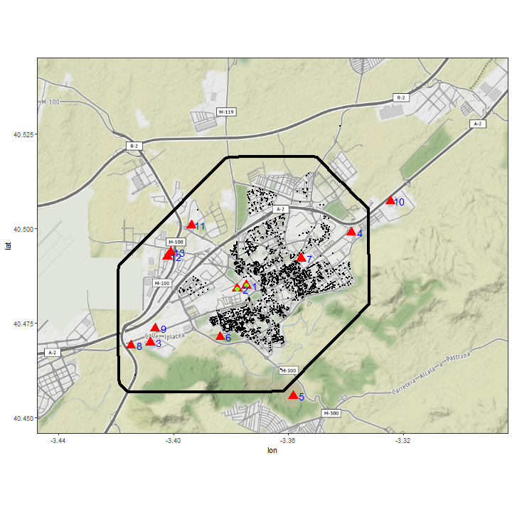
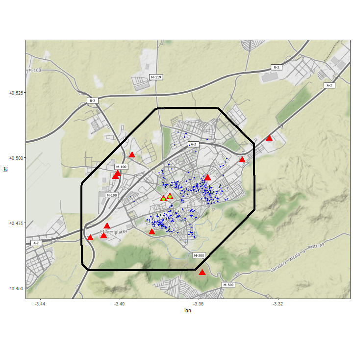
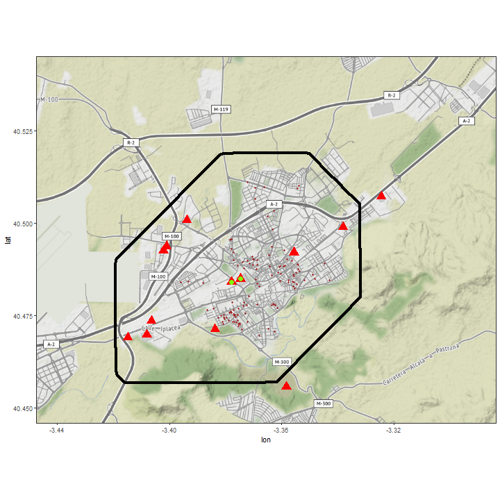
Figure 1: From top to bottom and left to right, locations of the controls and cases of lung, stomach and kidney cancer, respectively. The red triangles represent the locations of air polluting industries and green dots the locations of the heavy metals industries. The boundary represents the study region.

Figure 1 shows the locations of the cases and controls, as well as the locations of the polluting industries. It is clear that, while most of the polluting industries are outside the city, a few of them remain close to the city center.

An inhomogeneous Poisson point process will be assumed for each point type. The intensity of the controls at a location $x$ of the study area $\mathcal{D}$ will be represented by $\lambda_{0}(x)$, while the intensities of the cases of lung, stomach and kidney cancer will be represented by $\lambda_{i}(x),i=1,2,3$, respectively. Similarly, $n_{i},i=0,\ldots,3$ will represent the number of controls and cases of the different types of cancer.

A simple way to assess spatial variation is to compute ratios $\rho_{i}(x)=\lambda_{i}(x)/\lambda_{0}(x)$KelsallDiggle:1995SiM . In the case of no risk variation, the distribution of cases will follow that of the population, i.e., $\lambda_{i}(x)=\frac{n_{i}}{n_{0}}\lambda_{0}(x),i=1,2,3$. For this reason, under no spatial risk variation, ratio $\rho_{i}(x)$ will be equal to $n_{i}/n_{0}$.

In practice, the intensities involved need to be estimated, and these will be denoted by $\hat{\lambda}_{i}(x),i=0,\ldots,3$. A simple and popular estimate can be obtained with kernel smoothingDiggle:1985 . Note that in order to estimate the ratio of the intensities the same bandwidth of the kernel must be usedKelsallDiggle:1995Bern .

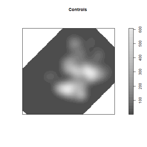
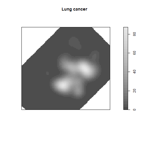
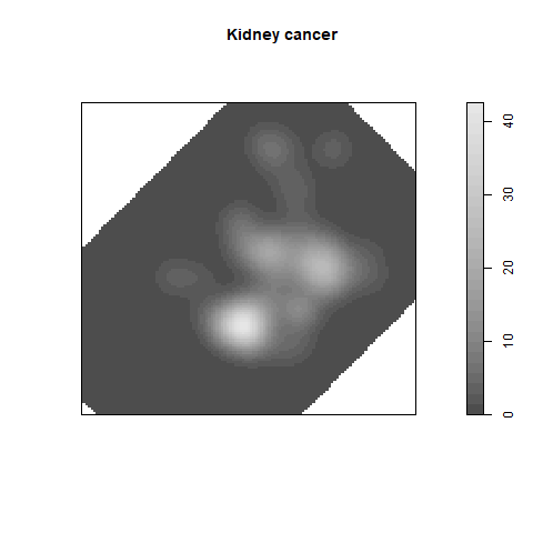
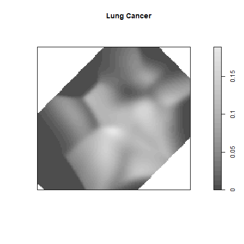
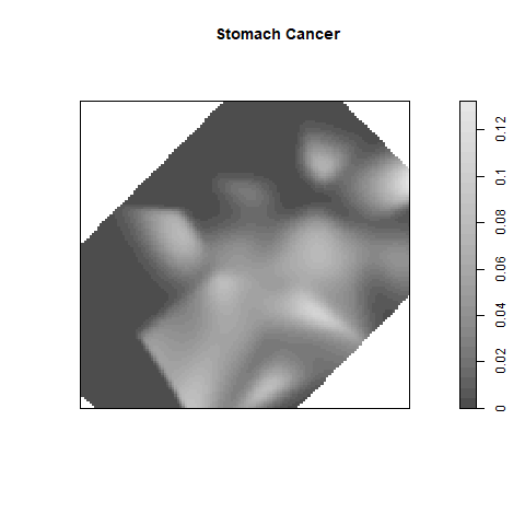
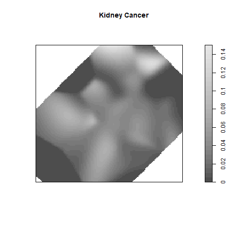
Figure 2: Estimated intensities of the controls $\hat{\lambda}_{0}(x)$ and the cases $\hat{\lambda}_{i}(x)=1,2,3$ (top row) and estimate of the ratio $\hat{\rho}_{i}(x),i=1,2,3$ (bottom row).

Figure 2 shows the estimates of the intensities for the three types of cancer $\hat{\lambda}_{i}(x)=1,2,3$ using a kernel smoothing with a bandwidth of 300 meters, together with the estimates of the ratio of the intensities $\hat{\rho}_{i}(x),i=1,2,3$. Note that, because of the different number of points, the intensity and relative risk estimates are in different scales.

The plots in Figure 2 are only presented as a summary of the spatial distribution of the point patterns, and the relative risk of the different types of cancer. A Monte Carlo test could be employed to find regions of significant high riskKelsallDiggle:1995SiM . Finally, a semi-parametric estimate of the intensities of the cases could be used in order to assess the impact of the covariates (and the locations of the polluting industries) in the spatial variation of the riskdiggle2007differences . These important issues will be addressed later within a Bayesian framework to develop a log-Gaussian Cox model which can account for the effect of the covariates and estimate the residual spatial variation of the risk.

3 Multivariate point patterns for disease mapping

Diggle et al. (2005)Diggleetal:2005 develop a suitable framework for the analysis of multivariate point patterns for the study of different strains of bovine tuberculosis. Each strain $i=1,\ldots,K$ is modeled using a different intensity $\lambda_{i}(x)$, and the probability of being a case of a strain of type $i$ at location $x$ is given by:

$$p_{i}(x)=\frac{\lambda_{i}(x)}{\sum_{j=1}^{K}\lambda_{j}(x)}$$

Our problem differs from the previous approach because, for case-control data, the intensity of the controls $\lambda_{0}(x)$ will act as a baseline in order to compare the intensity of the different types of diseases considered $\lambda_{i}(x),\ i=1,\ldots,K$. As mentioned above, for disease $i$, a relative risk could be computed as the ratio $\rho_{i}(x)=\lambda_{i}(x)/\lambda_{0}(x)$ and departures from the value $n_{i}/n_{0}$ will indicate significant spatial risk variation. Hence, this ratio can be used to describe spatial risk variation. Most importantly, it can help in the detection of hotspots by identifying regions of unusual high relative risk and assessing increased risk by exposure to pollution sources.

3.1 Spatial risk variation

As described in previous sections, spatial models for multivariate point patterns in Public Health should account for the spatial distribution of the population and address estimation of the effect of possible risk factors, putative pollution sources and any residual spatial variation not explained by previous factors.

First of all, our methodological proposal starts with a simple model to estimate the different intensities. In particular, the model proposed at a point $x$ of the study domain $\mathcal{D}$ is

$$\log(\lambda_{0}(x))=\alpha_{0}+S_{0}(x);x\in\mathcal{D}$$

$$\log(\lambda_{i}(x))=\alpha_{i}+S_{0}(x)+S_{i}(x),\ i=1,\ldots,K;x\in\mathcal{D}$$

where $\alpha_{i}$ is an intercept and $S_{i}(x)$ is a spatial Gaussian process with a Matérn covariance and $K$ is the number of diseases in the study. In general, the role of $\alpha_{i}$ is to account for the number of observed points and term $S_{0}(x)$ estimates the underlying spatial variation. Bayesian point estimates (e.g., the posterior means) of the intensities estimated by these models can be similar to the estimate obtained by kernel smoothing with the appropriate bandwidthTornadosVirgilio .

Note that the previous model is in fact a joint model and that $S_{0}(x)$ is estimated using cases and controls. Furthermore, it holds that

$$\log(\lambda_{i}(x))-\log(\lambda_{0}(x))=\alpha_{i}-\alpha_{0}+S_{i}(x),\ i=1,2,3;x\in\mathcal{D}$$ (1)

Hence, spatial effects $S_{i}(x),i=1,2,3$ measure any disease-specific residual spatial variation not accounted for by the distribution of the controls. As $S_{i}(x)$ measures departure from the spatial distribution of the controls, it can be used to detect areas of high risk by inspecting the credible intervals of its posterior distribution.

Gómez-Rubio et al. (2015)TornadosVirgilio propose a similar model in the context of a study on the spatial distribution of tornados according to their increasing strength (from 0 to 5) in the Contiguous United States. They consider 6 different types or tornados, with the mildest tornados providing a baseline intensity (i.e., tornados with intensity 0 acted as ’controls’). They plugged-in posterior estimates of the intensity of the tornados with intensity 0 as covariates to estimate the intensities of the other types of tornados. However, this ignores the uncertainty about the plugged-in intensity and the model proposed in this paper should be preferred to model multivariate point patterns within a Bayesian framework.

3.2 Exposure to pollution sources

If part of the spatial variation of the cases is thought to be explained by exposure to any of $P$ risk factors and the spatial distribution of the population, its intensity could be expressed asdiggle2007differences :

$$\lambda_{i}(x)=\lambda_{0}(x)\exp\{\alpha_{i}+\mathcal{F}_{ij}(x)+S_{i}(x)\},i=1,\ldots,K;j=1\ldots,P$$ (2)

Here, $\mathcal{F}_{ij}(x)$ is a generic term that represents exposure to a risk factor $j$ of a case of disease $i$, with $j=1,\ldots,P$. For exposure to pollution sources, this term usually depends on the distance to the location of the pollution source. The distance to the source for subject at location $x\in\mathcal{D}$ to the pollution source will be denoted by $d_{x}$. Note that this way of modeling exposure can be used without loss of generality to represent other risk factors, such as exposure to pollutants, temperature, body mass index, etc. and that it does not necessarily needs to be a distance.

Effect $\mathcal{F}_{ij}(x)$ can take several forms. First of all, a fixed effect can be considered, i.e., $\mathcal{F}_{ij}(x)=\beta_{ij}d_{x}$. This means that exposure is modeled as a fixed effect in the linear term and that each pollution source (or risk factor) $j$ affects differently each disease $i$. Negative values of $\beta_{ij}$ will indicate that the effect of the pollution source is to increase the intensity of the point pattern in its vicinity.

However, this is seldom a good idea as usually modeling risk factors requires a smoother termWood:2017 . For this reason, two other smooth models will be considered. The first one is a discrete random walk based on $r$ knots placed at distances $k_{1},\ldots,k_{r}$ from the pollution source. For a given disease $i$, the random walk associated to pollution source $j$ is defined as

$$u_{lj}-u_{l-1j}\sim N(0,\tau_{j});l=2,\ldots,r$$

with $\tau_{j}$ being a precision parameter. The effect is then defined as

$$F_{ij}(x)=u_{i(x)j}.$$

Here, $i(x)$ is an index that indicates the nearest knot to the case at location $x$. Hence, cases with similar distance to the pollution source will be allocated the effect of the same random walk term and their exposure will be similar.

The third effect will be a one-dimensional Gaussian process with a Matérn covariance based on the distance to the pollution source $j$. This is similar to the one used to model spatial effects $S_{i}(x)$ but using a single dimension.

In this case, the effect can be represented as

$$F_{ij}(x)=v_{ij}(x)$$

where $v_{ij}(x)$ is defined using a Gaussian process with zero mean and variance defined by a Matérn covariance in one dimension, where the values of the observations are the distances from the points to the pollution source.

Note that all these three possible ways of modeling the exposure to the pollution source can be extended to consider other risk factors which are measured using continuous variables such as, for example, blood pressure, weight, body-mass index, etc. Categorical risk factors, such as gender, can also be considered using fixed effects. Furthermore, note that different effects for different diseases are considered in our model, as exposure will likely have different effects on different diseases.

3.3 Detection of regions of high risk

Table 1 summaries four variations of the proposed model that can be fit to the data. Model 0 can be regarded as a baseline model for comparison as it assumes that the distribution of the cases and the controls is the same, and the intensities are scaled according to the values of $\alpha_{i},i=0,\ldots,K.$

Model 1 includes a disease-specific term $S_{i}(x)$ that accounts for unexplained spatial variation. If the distribution of the cases is exactly that of the controls, then this term should be equal to zero at every point of the study region. For this reason, the posterior distribution of $S_{i}(x)$ can be inspected for significant departures from zero, that will indicate regions of unexplained high risk. For example, credible intervals can be computed at grid points and then assess whether zero is inside. Alternatively, the posterior mean could be computed or the posterior probabilities of $S_{i}(x)$ being higher than zero could be computed as well (but this is computationally more expensive).

Model 2 assumes that all spatial variation of the cases is explained by that of the controls plus the effect of the risk factors. Model 3 adds a disease-specific spatial term to account for unexplained spatial variation, which can be used to assess regions of high risk not explained by the risk factors.

Ideally, model selection criteria should help to decide which model is best to explain the data. If either Model 1 (or Model 3) are selected it means that there is some residual variation not explained by the spatial distribution of the controls (and the risk factors)

Model	$\log(\lambda_{0}(x))$	$\log(\lambda_{i}(x))$
0	$\alpha_{0}+S_{0}(x)$	$\alpha_{i}+S_{0}(x)$
1	$\alpha_{0}+S_{0}(x)$	$\alpha_{i}+S_{0}(x)+S_{i}(x)$
2	$\alpha_{0}+S_{0}(x)$	$\alpha_{i}+S_{0}(x)+\mathcal{F}_{ij}(x)$
3	$\alpha_{0}+S_{0}(x)$	$\alpha_{i}+S_{0}(x)+\mathcal{F}_{ij}(x)+S_{i}(x)$

Table 1: Summary of models for multivariate point patterns using case-control data.

Furthermore, this joint modeling approach allows for the comparison of different disease-specific spatial terms, i.e., $\Delta_{uv}(x)=S_{u}(x)-S_{v}(x),\ u\neq v$, can be computed to assess similar residual spatial variation between two types of cancer. In the case of spatial residual variation, values of $\Delta_{uv}(x)$ close to zero will indicate a similar residual spatial variation which may point to common risk factors between two types of cancer.

4 Integrated Nested Laplace Approximation

Model fitting will be carried out using the integrated nested Laplace approximation (INLA)INLA . This approximation assumes that the model can be expressed as a latent Gaussian Markov random field (GMRF)RueHeld:2005 , i.e., the latent effects have Gaussian distribution with sparse covariance matrix that may depend on further hyperparameters. This includes some widely used models, such as, generalized linear and additive models with random effects. INLA will only provide approximations to the marginal posterior distributions of the model effects and hyperparameters, but this is often enough for inference.

INLA can fit models with latent spatial terms $S_{i}(x),i=0,\ldots,K$ that are defined using a Matérn covariance using the approximation based on stochastic partial differential equations (SPDE)SPDE ; Krainskietal:2019 . Furthermore, the multivariate point patterns model will be implemented using a representation of the cases and the controls as a Poisson processSPDELog-GausianCox .

The Matérn covariance between two points $x_{1}$ and $x_{2}$, separated by a distance $d_{12}$, is defined as

$$Cov(x_{1},x_{2})=\sigma^{2}\frac{2^{1-\nu}}{\Gamma(\nu)}(\kappa d_{12})^{\nu}K_{\nu}(\kappa d_{12})$$

Here, $\sigma^{2}$ is a variance parameter, $\kappa$ a spatial scale parameter and $\nu$ a smoothness parameter. Furthermore, $\Gamma(\cdot)$ is the Gamma function and $K_{\nu}(\cdot)$ is the modified Bessel function of the second kind.

The SPDE approximationSPDE to estimate a Gaussian process with Matérn covariance $S(x)$ implemented is based on a weak solution to a SPDE, so that the estimated effect is expressed as

$$S(x)=\sum_{k=1}^{m}\psi_{k}(x)w_{k}$$

Here, $\psi_{k}(x)$ are a basis of functions and $w_{k}$ are Gaussian weights. $k$ represents the number of vertices in a triangulation that covers the study region. This triangulation is used to define the basis functions as each function is piecewise linear within each triangle. In particular, $\psi_{k}(x)$ is equal to 1 at vertex $k$ and 0 at all other vertices. This provides a sparse representation that is very convenient in practice for computational purposes. When reporting the results, the nominal variance and the nominal range, will be used to summarize the estimates of the spatial effects $S_{i}(x),i=0,\ldots,K$.

Fitting log-Gaussian Cox processes to point patterns with INLA is based on reformulating the model as a Poisson regressionSPDELog-GausianCox . This requires creating a Voronoi tessellation using the observed points of the point pattern. For each polygon, a dummy observation with value 0 and associated value $A_{k}$, the area of the associated polygon, is added, and each observed point is added with a value 1 and $A_{k}$ equal to 0. Then, the model is a Poisson regression as follows:

$$y_{k}\sim Po(A_{k}\theta_{k}),k=1,\ldots$$

Here, $y_{k}$ are the 0/1 values described above, $A_{k}$ the area of the associated polygon and $\theta_{k}$ accounts for the model effects. For example, for Model 3 and disease $i$ this would be:

$$\log(\theta_{k})=\alpha_{i}+S_{0}(x_{k})+\mathcal{F}_{ij}(x_{k})+S_{i}(x_{k})$$

where $x_{k}$ is the location of observed or dummy point $x_{k}$.

Note that, in order to fit this model with INLA, the covariates associated to the risk factors need to be available at the dummy points. This is not a problem when they are distances to pollution sources, but it could be a problem when the risk factor is an individual level variable, such as gender or age.

In practice, implementing this joint model requires the use of different likelihoods, one for each point pattern, with a shared effect $S_{0}(x)$. This is fully described in the R code used in this paper, which is available from Github at https://github.com/becarioprecario/INLA_MVPP.

5 Spatial variation of cancer in Alcalá de Henares (Madrid, Spain)

We have analyzed the data introduced at the beginning of the paper on cancer data from Alcalá de Henares (Madrid, Spain) using the model introduced above. In order to fully describe the model, the priors on the different parameters must be stated. Priors on the fixed effect have been a Gaussian distribution with zero mean and precision 1000. We have used PC-priors (Simpsonetal:2017, ) for the parameters of the SPDE-based spatial effects. In particular, the prior on the range is so that $P(range<5)=0.95$ and the prior on the standard deviation $\sigma$ is so that $P(\sigma>10)=0.01$. These setting are based on reasonable vague assumptions about the underlying spatial processes.

5.1 Confounding factors

When assessing increased risk around pollution sources it is important to account for other factors that may play a role in the spatial distribution of the disease. For example, socioeconomic indicators (e.g., income or education) or life style (e.g., diet or smoking status) may drive the spatial pattern for some diseases. For example, lung cancer is highly correlated with income and smoking(Faggianoetal:1997, ; Spitzetal:2006, ).

For this reason, the models presented here can include fixed effects on some covariates. Note that given the multivariate nature of our models it is important to allow for disease-specific coefficients for the fixed effects because different risk factors can affect the diseases under study in different ways.

Furthermore, our analysis will consider models that do not account for risk factors first. Then, models that account for confounding factors will be fit to assess whether the effects from pollution sources are still significant. This will allow us to determine whether the primary cause of increased mortality is due to the pollution source or socio-economic confounding variables.

In particular, the variables that we have considered are available at the census tract level, obtained from the 2001 Spanish census by Instituto Nacional de Estadística (INE, Spain). Values have been assigned to the cases or the controls by matching the census tract. The variables considered are unemployment rate in the range between 20 and 59 years (UNEMP2059), an average of the score for social class (AVGSOC), an average of the score for education level in the range between 30 and 39 (AVGEDU) and the percentage of children aged between 0 and 3 that are in the school (PCTSCH).

5.2 Spatial risk variation

The first step in our analysis of the three types of cancer in Alcalá de Henares will be to inspect spatial risk variation in order to assess whether the spatial distributions of the cancers is the same as the controls. For this, we have fit models 0 and 1, and we have computed some model selection measures in order to make a decision on the best model. Models 2 and 3 are discussed later as they will depend on the pollution sources included in the model.

	No confunding			With confunding
	factors			factors
Model	DIC	WAIC	Marg. lik.	DIC	WAIC	Marg. lik.
0	-31454.12	-28463.91	15558.89	-31441.31	-28390.93	15494.42
1	-31486.21	-28365.77	15560.84	-31479.50	-28263.28	15498.55

Table 2: Model selection criteria values for the different models fit to the case-control data.

Table 2 summarizes the different criteria computed with INLA. For models without confounding factors, the DIC and marginal likelihood support Model 1, i.e., that there is disease-specific spatial variation not explained by the spatial distribution of the controls. Models that include confounding factors do not seem to improve model fitting. Table 3 shows the effects of the covariates. In particular, high unemployment and children in school are close to have a significant positive association with the three types of cancer. On the other hand, education level and social level does not seem to have an effect.

These four covariates where taken not to be correlated with each other but it is possible that some confounding is occurring when all four are in the model, and this might be the reason why all credible intervals contain the zero value and model selection criteria do not favor models with confounding factors included. In any case, by including these four covariates typical possible socio-economic confounders are taken into account and we have kept all four variables in all models that include confounding factors.

Variable	Cancer	Model 0				Model 1
		Mean	St. dev.	95% C.I.		Mean	St. dev.	95% C.I.
UNEMP2059	lung	0.03	0.03	-0.02	0.09	0.06	0.03	-0.00	0.13
UNEMP2059	stomach	0.05	0.04	-0.03	0.13	0.09	0.05	-0.01	0.18
UNEMP2059	cancer	0.06	0.05	-0.03	0.15	0.08	0.05	-0.02	0.18
AVGSOC	lung	0.80	1.07	-1.30	2.91	1.81	1.19	-0.51	4.16
AVGSOC	stomach	-0.30	1.58	-3.38	2.81	0.86	1.75	-2.55	4.33
AVGSOC	cancer	0.01	1.67	-3.25	3.32	0.62	1.83	-2.90	4.27
AVGEDU	lung	-0.11	0.35	-0.79	0.57	-0.21	0.40	-0.99	0.58
AVGEDU	stomach	0.21	0.50	-0.78	1.20	-0.10	0.57	-1.23	1.01
AVGEDU	cancer	0.47	0.55	-0.61	1.53	0.31	0.60	-0.90	1.47
PCTSCH	lung	0.01	0.01	-0.00	0.02	0.01	0.01	-0.00	0.3
PCTSCH	stomach	0.00	0.01	-0.01	0.02	0.01	0.01	-0.01	0.03
PCTSCH	cancer	0.01	0.01	-0.01	0.03	0.02	0.01	-0.01	0.04

Table 3: Estimates of the confounding factors included in the models for Models 0 and 1.

Table 4 summarizes the spatial effects $S_{i}(x)$ of the different models. This table is useful to compare the estimates of effect $S_{0}(x)$ between the different models. When no confounding factors are included, we find very similar estimates of the parameters of $S_{0}(x)$ in both models. Under Model 1 stomach cancer seems to have the highest nominal standard deviation and nominal range of the disease-specific spatial effect, which may point to a differential spatial variation. On the other hand, kidney cancer has the smallest nominal variance and range, which may point to a lack of differential spatial distribution. Finally, the estimates of the parameters for the spatial effect of lung cancer point to a possible mild differential spatial variation.

When confounding factors are included, the spatial effect in Model 0 has very similar estimates as the case with no confounding factors. However, Model 1 shows smaller estimates of the range for the disease-specific spatial effects. In our opinion, this is due to the socio-economic confounding variables included in the model, that account for some of the spatial variation in the data.

Model	Cancer	Conf. factor	Nominal Range		Nominal St. dev.
			Mean	St. dev.	Mean	St. dev.
0	Controls	No	3.94	1.13	4.06	1.08
1	Controls	No	3.89	1.16	3.99	1.10
1	Lung	No	6.64	6.52	0.76	0.44
1	Stomach	No	6.91	6.08	0.85	0.51
1	Kidney	No	3.00	8.76	0.22	0.15
0	Controls	Yes	3.93	1.12	4.04	1.07
1	Controls	Yes	3.88	1.09	4.00	1.04
1	Lung	Yes	4.00	2.70	0.60	0.22
1	Stomach	Yes	5.56	4.40	0.86	0.38
1	Kidney	Yes	1.45	1.64	0.33	0.17

Table 4: Summary of the spatial effects of the different models fit to the case-control data.

Because of this small sample size, detecting departures from Model 0 will be difficult. Given the nature of the problem at hand, it is not easy to increase the sample size, and the only reason to do this is to extend the period of time of the analysis, which is not always possible. A similar problem will be faced when assessing exposure to pollution sources. For this reason, a simulation study will be developed at the end of this section.

5.3 Detection of regions of high risk

Given that the underlying spatial variation $S_{0}(x)$ is taken as a baseline as it represents the distribution of the controls, the detection of the areas of high risk can be tackled by looking at which points in the study region have high (or low) values of $S_{i}(x)$ using its posterior distribution $\pi(S_{i}(x)|y)$. We will inspect this by looking at the credible intervals of the estimates of the disease-specific effects computed at a grid of points inside the study region. Departures from the null value will indicate regions of high or low intensity.

Figure 3 displays posterior means and standard deviations of the spatial effects $S_{i}(x)$ for the different types of cancer obtained by fitting Model 1 and accounting for confounding factors. In the plots, point estimates and credible intervals have been arranged in increasing order (using the posterior mean). These intervals can be used to assess whether residual spatial variation has a high probability of being different from zero, which will indicate a departure in the cases from the spatial distribution of the controls.

The estimates provided by Model 1 without adjusting for confounding factors are similar, but with wider credible intervals (and they have not been included here). The reduction of the width of the credible intervals is then due to the effect of the covariates. Because of the small sample size, we believe that credible intervals are not narrow enough as to detect hostspots due to the polluting industries. For these reasons, we have decided to consider the models that include exposure to pollution sources in the analysis.

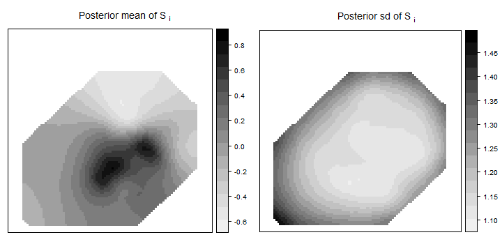
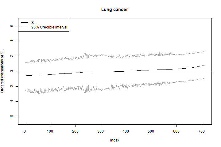
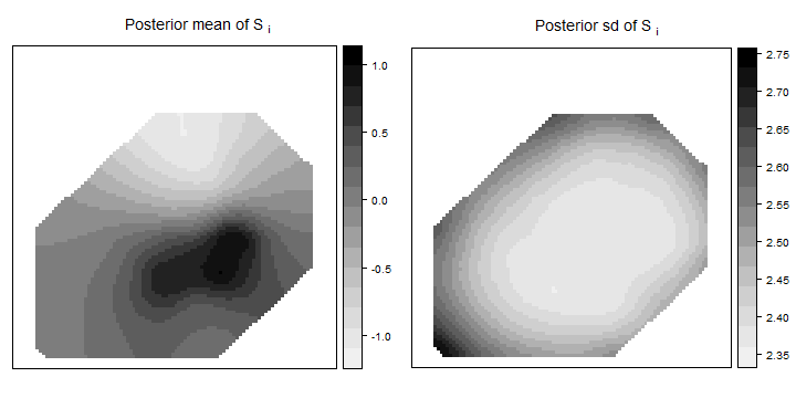
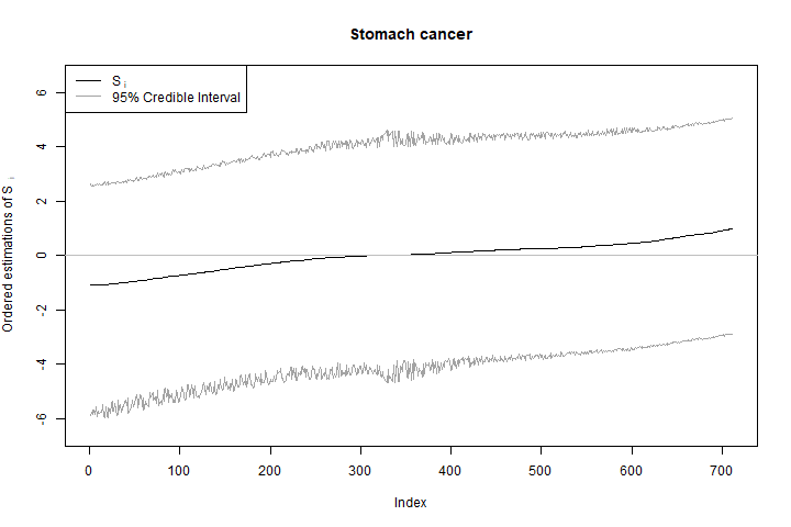
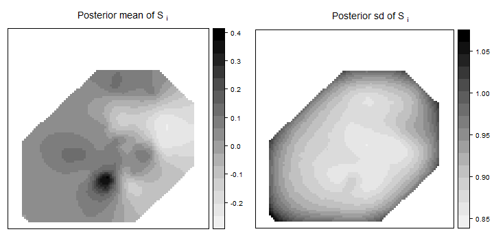
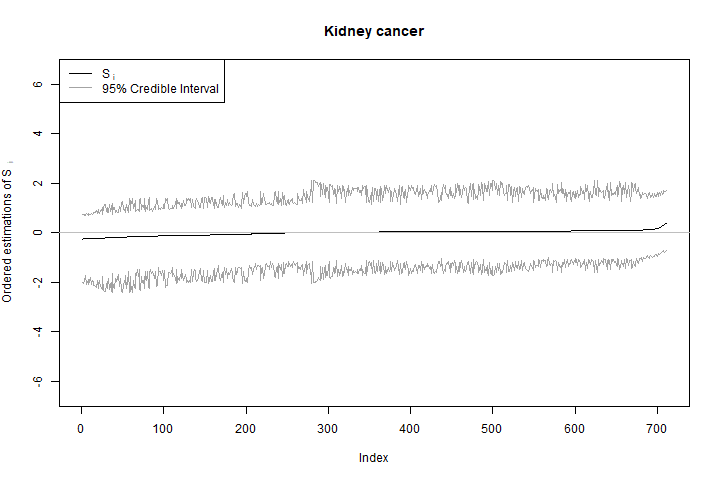
Figure 3: Summary statistics of spatial effects $S_{i}(x)$: map of posterior means (top row), posterior means and 95% credible intervals (middle row) and map of posterior probabilities $\pi(S_{i}(x)>0|y)$.

For kidney cancers, all credible intervals contain the zero value, which indicates no departure from the underlying spatial distribution of the controls. However, lung and stomach cancers have higher point estimates of $S_{i}(x)$ and they are close to having smaller regions with high values of the disease-specific spatial term. This indicates spatial variation not accounted for the spatial distribution of the controls. Note how these regions seem to be close to the south part of the city. Hence, we believe that it is important to test for a possible association between this increased intensity in the cases and the location of industries. This is carried out below, using models 2 and 3.

5.4 Assessing exposure to pollution sources

We will inspect a possible association between the location of the industries in the city and an increased intensity about them. Full details about the estimates for the different models are included in the Supplementary Materials of this paper. In the analysis of these results, we will focus on the models that point to an increased risk around polluting industries. For this reason, model selection will not only be based on the DIC and WAIC criteria but also on reasonable estimates of the spatial effects in the model and on estimates of the effect $\mathcal{F}_{ij}(x)$ that points to an increased risk around the pollution source. Note that some estimates of the DIC and WAIC were not reliable and they have been replaced by a dash in some of the tables in this paper.

Table 5 shows estimates of the DIC and WAIC for the different models (not adjusted for confounding variables) to assess risk around pollution sources using a fixed effect, a RW1 and a SPDE1. This table also summarizes for which diseases there is an increased risk. The inclusion criterion has been a negative upper limit of the 95% credible interval of the coefficient for fixed effect, or a decreasing trend with distance when the effect is either a RW1 or SPDE1 smooth term (even if the 95% credible intervals contained the zero value). The top plots in Figure 4 show an example of the inclusion criteria used to list a tumor in Table 5. Note that the descending trend with distance is clear, but that for the RW1 and SPDE1 effects 95% credible intervals contain the zero value. However, we believe this is simply due to the small sample size that we have in our particular dataset.

In addition to the previous criteria, values of the DIC and WAIC smaller than the ones obtained for Model 0 and 1 will indicate a significant effect. This is associated with a credible interval for the fixed effect that is above zero, and effects RW1 and SPDE1 showing a decreasing pattern around the pollution sources, such as the one seen in Figure 4 (for Industry 1).

We have not reported here the estimates of the different spatial effects in the model because, in general, these are very close to the obtained for Models 0 and 1. In any case, these are provided in the Supplementary Materials of this paper. The results indicate that seven industries have a potential association with an increase of the intensity of different types of cancer around them. This is particularly clear for lung and stomach cancer, while this possible association with kidney cancer is very mild or inexistent.

Given that this increase may also be due to socio-economic factors, we have fit the same models with the four socio-economic variables mentioned above. In general, the estimates of the coefficients are very similar to those obtained for Models 0 and 1, and they are not reported here (but they have been included in the Supplementary Materials). Table 6 shows a summary of the DIC and WAIC for these models, that includes for which types of cancer there is a significant increase around the pollution source. As mentioned earlier, Model 3 has not been included here because we suspect that the different effects in the model are not identifiable as we are accounting for confounding factors and including disease-specific spatial terms.

Values of the DIC are smaller when adjusting for confounding factors. However, WAIC seems to increase. When assessing exposure, models with RW1 and SPDE1 are preferred over models with fixed effects. In general, the associations detected by the different models are very similar to the case with no adjustment, which means that there is still a possible association between an increase in the number of cases and the distance to the polluting industries. This association is clear for lung and stomach cancer, and very mild (or inexistent) for kidney cancer.

Regarding the industries that appear in Table 5 and Table 6, Industries 1 and 2 are part of an industrial area very close to the city center. The presence of asbestos in this area could explain the apparent increase in the cases of lung and stomach cancer. Industry 5 is a landfill, where waste is often cremated and the smoke reaches the population at kilometers away. Industry 6 is close to a deprived area, which could be the case of this increase in the cases of cancer but we have already accounted for several socioeconomic variables. Industries 7, 8 and 9 do not show any association for the models with RW1 and SPDE1 effects and we believe that there is in fact no association with cancer.

Given that our study is limited by the small sample size of the cases and the four socio-economic variables included in the model, we want to be cautious about pointing to any significant association between the increase of cases of cancer around the aforementioned industries. However, we believe that the new methodology developed in this paper is appropriate for the task at hand.

		Model 2			Model 3
Source	Effect	DIC	WAIC	Tumour	DIC	WAIC	Tumour
Industry 1	Fixed	-31576.57	-28523.96	L, S	-31604.58	-28446.86	L, S
Industry 2	Fixed	-31575.79	-28522.54	L, S	-31605.73	-28444.19	L, S
Industry 5	Fixed	-31576.32	-28525.60	L, S	-31598.35	-28432.65	–
Industry 6	Fixed	-31574.03	-28516.32	L, S, K	-31603.99	-28440.13	L
Industry 7	Fixed	-31561.54	-28501.01	–	-31605.74	-28438.69	L
Industry 8	Fixed	-31565.95	-28509.09	L, K	-31599.19	-28435.79	–
Industry 9	Fixed	-31566.34	-28509.38	L, K	-31599.81	-28436.22	–
Industry 1	RW1	-31563.00	-28491.15	L	-31604.58	-28446.86	L, S
Industry 2	RW1	-31621.04	-27630.06	L	-31605.73	-28444.19	L, S
Industry 5	RW1	-31618.46	-28490.14	L, S	-31598.35	-28432.65	L, S
Industry 6	RW1	-31557.60	-28497.06	L	-31603.99	-28440.13	L, S
Industry 7	RW1	-31559.55	-28519.13	–	-31605.74	-28438.69	–
Industry 8	RW1	-31559.63	-28515.80	–	-31599.19	-28435.79	–
Industry 9	RW1	-31559.61	-28515.22	–	-31599.81	-28436.22	–
Industry 1	SPDE1	-28613.62	–	L, S	–	–	L, S
Industry 2	SPDE1	-31573.44	-28447.03	L, S	–	–	L, S
Industry 5	SPDE1	-31606.01	–	L, S	-31590.59	–	L, S
Industry 6	SPDE1	-31590.62	-28438.07	L	-31604.02	-28376.68	–
Industry 7	SPDE1	-31568.83	-28451.21	—	-31600.12	-28398.24	–
Industry 8	SPDE1	-31567.08	-28448.97	—	-31594.16	-28384.54	–
Industry 9	SPDE1	-31565.64	-28454.97	—	-31593.62	-28294.52	–

Table 5: Summary of Models 2 and 3 (without confounding factors) to assess exposure around polluting industries.

		Model 2
Source	Effect	DIC	WAIC	Tumour
Industry 1	Fixed	-31624.75	-28461.34	L, S, K
Industry 2	Fixed	-31623.27	-28461.01	L, S, K
Industry 5	Fixed	-31598.99	-28449.47	L, S, K
Industry 6	Fixed	-31609.41	-28451.30	L, S, K
Industry 7	Fixed	-31585.11	-28429.39	K
Industry 8	Fixed	-31600.10	-28445.24	L, K
Industry 9	Fixed	-31601.54	-28445.97	L, K
Industry 1	RW1	-31645.50	–	L, S
Industry 2	RW1	-31734.66	–	L, K
Industry 5	RW1	-31657.11	-28415.90	L, S
Industry 6	RW1	-31773.61	–	L, S
Industry 7	RW1	-31583.83	-28451.82	–
Industry 8	RW1	-31613.32	-28388.08	L
Industry 9	RW1	-31609.66	-28381.25	L
Industry 1	SPDE1	-31626.01	–	L, S
Industry 2	SPDE1	-31632.65	–	L, S
Industry 5	SPDE1	-31661.90	–	L, S
Industry 6	SPDE1	-31682.90	-28289.75	–
Industry 7	SPDE1	-31619.81	-28375.44	–
Industry 8	SPDE1	-31622.06	-28370.71	–
Industry 9	SPDE1	-31619.74	-28353.05	–

Table 6: Summary of Model 2 (with confounding variables) to assess exposure around polluting industries.

Given that Model 2 seems to be the best model for RW1 and SPDE1 effects, we have displayed the estimates of the effects for Industry 1 in Figure 4. The estimated effects are similar between RW1 and SPDE1 effects, with a step-like effect for lung and stomach cancer. This is consistent with the fact that this pollution source is close to the city center. The effect on kidney cancer is negligible. Similar figures for all the other pollution sources are available in the Supplementary Materials.

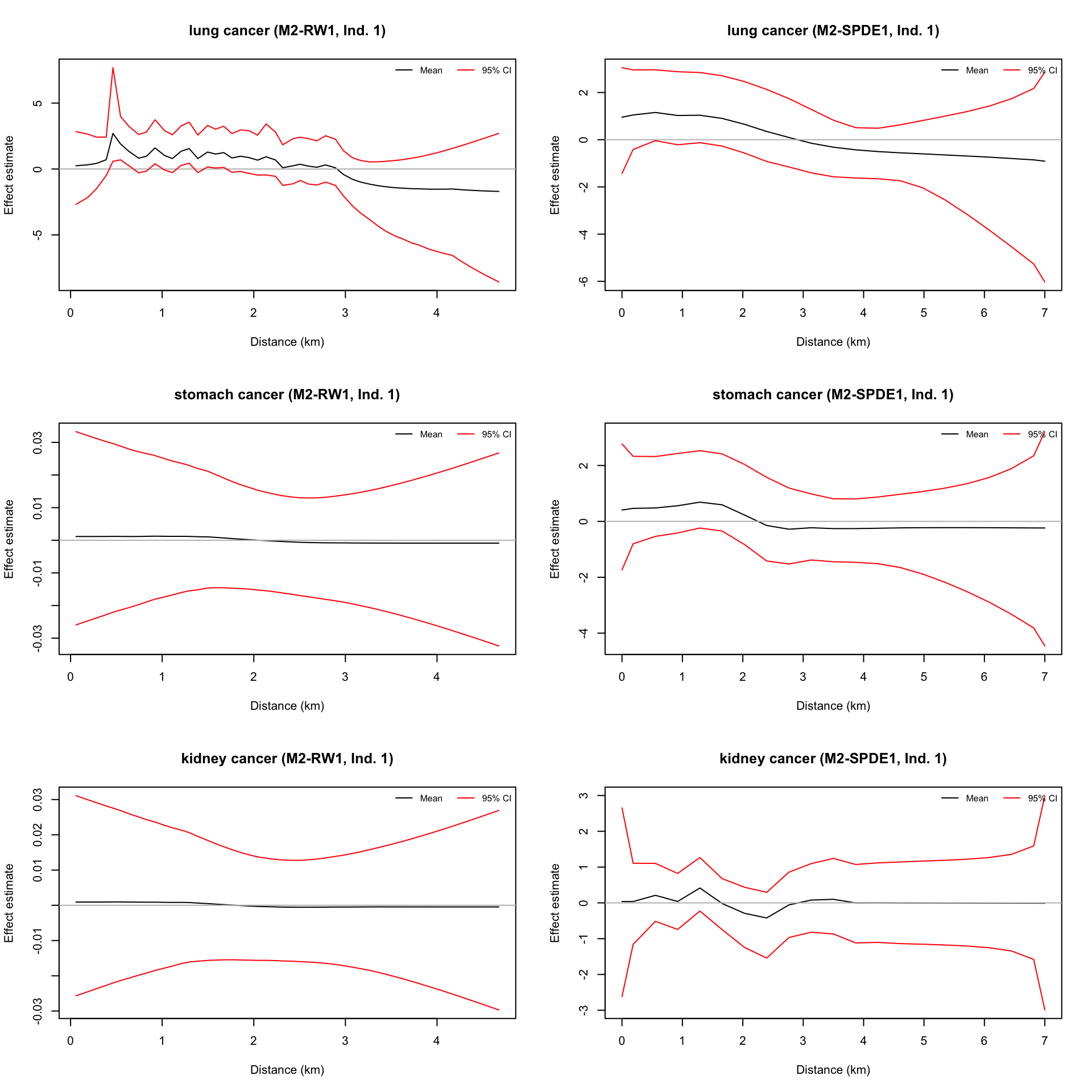
Figure 4: Estimated effects of Model 2 for the effect of the proximity to industry 1 using RW1 (left) and SPDE1 (right) smooth effects.

Detection of the effect produced by the pollution sources and other risk factors depends on the sample size of the data. In epidemiological studies it is seldom possible to increase the sample size of the cases and the association between risk factors and the disease may not be detected because of a small sample size. For this reason, we have conducted a simulation study in the next section to assess how the estimates of the effects depend on the sample size of the cases. In particular, we will pay attention to point estimates (i.e., posterior means) and 95% credible intervals.

5.5 Simulation study

In order to assess how sample size impacts the detection of effects due to risk factor using the the three forms of function $\mathcal{F}_{ij}(x)$, a simulation study has been carried out. In particular, we have simulated a new set of 3000 controls from the estimated intensity of the actual controls, and then we have simulated a set of cases using the estimated intensity of the simulated controls modulated by an effect that depends on the distance to a pollution source using an exponential decay function. Note that cases from a single disease are considered now instead of cases from several diseases. Also, the putative pollution source used in the simulations is located where Industry 1 is (see Figure 1).

This means that the intensity of the simulated cases is

$$\hat{\lambda}_{0}(x)\exp\{-d_{x}/\phi\}$$

where $\hat{\lambda}_{0}(x)$ is the estimated intensity of the simulated controls, $d_{x}$ the distance (in kilometers) to the pollution source and $\phi$ a scale parameter are parameters to measure how the intensity of the cases is modulated by the distance to the pollution source.

Data have been simulated using values of $\phi$ of 1, 3 and 6, and the number of simulated cases have been 50, 100, 300, 500, 1000 and 2000. The number of simulated controls has always been 3000. Distances from the simulated points to the pollution source range from 0.05 to 5.3, approximately. Hence, for a value of $\phi$ equal to 1 we can expect a fast decay, while a value of 6 will produce a slow decay of the effect of the pollution source (and very similar effects of the source on the intensity of all the controls).

Table 7 shows the values of the DIC for Models 2 and 3 fit to the simulated data using RW1 and SPDE1 effects on the distance to the pollution source. RW1 models point to Model 2 in most cases and, in particular, for large sample sizes and large values of $\phi$. SPDE1 models show very similar values for both models, which would lead to selecting Model 2 (as this is simpler).

In general, for $\phi$ equal to 6 both models provide similar values of the DIC for both RW1 and SPDE1. This is consistent with a situation in which the pollution source has a negligible effect.

Hence, detectability of the effect produced by the proximity to the pollution source increases with sample size and the strength of the effect on the proximity. For a conveniently large sample size, the models presented in this paper are able to detect exposure to a pollution source, even when this effect is mild.

Settings				RW1		SPDE1
# Cases	$\varphi$	M0	M1	M2	M3	M2	Model 3
50	1	-22812.90	-22831.77	-22838.29	-22831.98	-22839.07	-22839.12
50	3	-22796.62	-22796.39	-22796.93	-22796.62	-22800.88	-22800.81
50	6	-22796.41	-22796.12	-22796.74	-22796.15	-22796.29	-22795.99
100	1	-22934.97	-22965.97	-22967.99	-22965.95	-22976.62	-22976.27
100	3	-22911.74	-22913.33	-22912.16	-22912.62	-22921.13	-22920.72
100	6	-22908.13	-22907.91	-22908.53	-22908.13	-22911.90	-22911.18
300	1	-23880.00	-24028.13	-24035.86	-24028.87	-24049.91	-24049.47
300	3	-23797.38	-23815.83	-23819.03	-23819.15	-23825.43	-23824.90
300	6	-23774.33	-23777.53	-23781.62	-23777.52	-23782.49	-23782.12
500	1	-25126.22	-25388.90	-25400.31	-25421.05	-25420.41	-25420.22
500	3	-24946.51	-24970.60	-24978.07	-24975.04	-24981.11	-24980.70
500	6	-24920.53	-24925.79	-24936.79	-24934.07	-24936.19	-24934.67
1000	1	-28835.55	-29245.86	-29268.02	-29303.88	-29287.42	-29286.82
1000	3	-28459.73	-28503.98	-28516.88	-28512.76	-28519.96	-28519.22
1000	6	-28341.42	-28341.35	-28353.58	-28345.77	-28352.02	-28351.56
2000	1	-37725.47	-38356.53	-38367.91	-38443.95	-38415.57	-38415.05
2000	3	-36795.54	-36850.21	-36870.57	-36866.91	-36874.63	-36874.02
2000	6	-36604.24	-36604.09	-36617.14	-36613.30	-36617.83	-36617.49

Table 7: Values of the DIC for the models fit to the simulated data.

Figure 5 shows the estimates of the smooth terms using SPDE1 effects for different values of the sample size and $\phi$ equal to 3. The estimated effects are similar for RW1 effects and they are not shown. As it can be seen, the detectability of the effects increases with the sample size, and the credible intervals get narrower with the sample size. Results are similar for $\phi$ equal to 6, which produces a stronger effect and thus detecting a significant effect requires a smaller sample size.

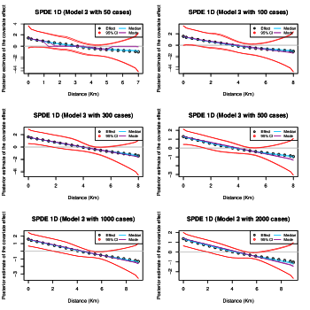
Figure 5: Estimated effect of a pollution source using Model 2 and SPDE1 effects on the simulated case-control data with $\phi$ equal to 3.

Model 3 did not detect exposure to the pollution source in any of the simulated scenarios. This is probably due to the fact that the disease-specific spatial terms accounts for all the unexplained spatial variation. This points to a possible confounding between disease-specific spatial pattern $S_{i}(x)$ and the effect on the covariates $\mathcal{F}_{ij}(x)$. Hence, Model 2 will be preferred in case of doubt.

6 Discussion

The integrated nested Laplace approximation is a suitable Bayesian inferential framework to fit log-Gaussian Cox processes to multivariate point patterns. The log-intensity can be modeled as a sum of fixed effects and smooth terms on the covariates plus spatial smooth terms using the SPDE approximation. Hence, models for multivariate point patterns can be developed with ease.

These models have been applied to case-control data where cases of several types of cancer have been considered. The models proposed in this paper have been adequate to assess spatial risk variation and the detection of regions of high risk. Furthermore, the assessment of risk due to the proximity to putative pollution sources can be assessed by considering the distance from the cases to the pollution source. Finally, this methodology can be used to assess differences in the disease-specific residual spatial variation between two diseases. This can be of interest to identify diseases with a similar spatial variation.

These models have been applied to a dataset from Alcalá de Henares (Madrid, Spain) to study the spatial risk variation of lung, stomach and kidney cancer using case-control data. These models have been able to identify a (mild) disease-specific spatial variation for lung and stomach cancer, while the distribution of cases of kidney cancer seems to follow that of the controls. Models with shared and disease-specific spatial pattern have been able to highlight the regions of high risk for lung and stomach cancer. Furthermore, by including the effect of the distance to important pollution sources around the city we have been able to identify some possible sources of pollution that affect the location of cases of lung and stomach cancer. A further epidemiological study could look at the particular activity of each industry and how that could be possibly linked to the increase of cancer cases.

Although this study is limited by the small number of cases available and the effect of the distance to the pollution source was difficult to assess, we have carried out a simulation study that confirms that this methodology can detect the effect of risk factors, such as exposure to pollution sources.

In the future, we expect to extend the current methodology to perform automatic detection of socio-economic risk factors as well as the effect of pollution sources. This can be done by using Reversible Jump MCMCGreen:1995 methods so that the effects on the pollution sources can be automatically included (or removed) from the model.

This methodology can also be extended to the spatio-temporal case by modeling the log-intensity as the sum of a spatial effect plus a temporal effect, using a RW1 or SPDE1 effects(Krainskietal:2019, ). Covariates could also be considered in this model as well.

7 Acknowledgments

This work has been supported by grants PPIC-2014-001-P and SBPLY/17/180501/000491, funded by Consejería de Educación, Cultura y Deportes (JCCM, Spain) and FEDER, and grant MTM2016-77501-P, funded by Ministerio de Economía y Competitividad (Spain).

F. Palmí-Perales has been supported by a Ph.D. scholarship awarded by the University of Castilla-La Mancha (Spain).

The authors thank Mario González-Sánchez and Javier González-Palacios (”Bioinformatics and Data Management Group” (BIODAMA, ISCIII)) for their technical support in data base maintenance.

Disclaimer: This article presents independent research. The views expressed are those of the authors and not necessarily those of the Carlos III Institute of Health.

References

- (1) Diggle P. Statistical analysis of spatial point patterns. 2nd ed. Arnold, 2003.
- (2) Diggle PJ, Gómez-Rubio V, Brown PE et al. Second-order analysis of inhomogeneous spatial point processes using case–control data. Biometrics 2007; 63(2): 550–557.
- (3) PJ D and B R. A conditional approach to point process modelling of elevated risk. Journal of the Royal Statistical Society, Series A 1994; 3(157): 433––440.
- (4) Gelfand AE, Diggle P, Guttorp P et al. Handbook of spatial statistics. CRC press, 2010.
- (5) Baddeley A, Rubak E and Turner R. Spatial point patterns: methodology and applications with R. CRC Press, 2015.
- (6) Diggle PJ, Moraga P, Rowlingson B et al. Spatial and spatio-temporal log-gaussian cox processes: extending the geostatistical paradigm. Statistical Science 2013; : 542–563.
- (7) Diggle PJ, Zheng P and Durr P. Nonparametric estimation of spatial segregation in a multivariate point process: bovine tuberculosis in cornwall, uk. Journal of the Royal Statistical Society, Series C 2005; 54(3): 645–658.
- (8) Rue H, Martino S and Chopin N. Approximate bayesian inference for latent gaussian models by using integrated nested laplace approximations. Journal of the royal statistical society: Series b (statistical methodology) 2009; 71(2): 319–392.
- (9) Lindgren F, Rue H and Lindström J. An explicit link between gaussian fields and gaussian markov random fields: the stochastic partial differential equation approach. Journal of the Royal Statistical Society: Series B (Statistical Methodology) 2011; 73(4): 423–498.
- (10) Simpson D, Illian JB, Lindgren F et al. Going off grid: Computationally efficient inference for log-gaussian cox processes. Biometrika 2016; 103(1): 49–70.
- (11) Fernández-Navarro P, López-Abente G, Salido-Campos C et al. The minimum basic data set (mbds) as a tool for cancer epidemiological surveillance. European Journal of Internal Medicine 2016; 34: 94 – 97. https://doi.org/10.1016/j.ejim.2016.06.038. URL http://www.sciencedirect.com/science/article/pii/S0953620516302187.
- (12) Fernández-Navarro P, Sanz-Anquela JM, Ángel Sánchez-Pinilla et al. Detection of spatial aggregation of cases of cancer from data on patientsand health centres contained in the minimum basic data set. Geospatial health 2018; 13(616): 86–92.
- (13) Fernández de Larrea-Baz N, Álvarez-Martín E, Morant-Ginestar C et al. Burden of disease due to cancer in spain. BMC Public Health 2009; 42(9): 1–11.
- (14) Fernández-Navarro P, García-Pérez J, Ramis R et al. Industrial pollution and cancer in spain: An important public health issue. Environmental research 2017; 159: 555–563.
- (15) E KJ and J DP. Non-parametric estimation of spatial variation in relative risk. Statistics in Medicine 1995; 14(21–22): 2335–2342. 10.1002/sim.4780142106. URL https://onlinelibrary.wiley.com/doi/abs/10.1002/sim.4780142106. https://onlinelibrary.wiley.com/doi/pdf/10.1002/sim.4780142106.
- (16) Diggle PJ. A kernel method for smoothing point pattern data. Applied Statistics ; 34: 138–147.
- (17) E KJ and J DP. Kernel estimation of relative risk. Bernoulli ; 1(1–2): 3–16.
- (18) Gómez-Rubio V, Cameletti M and Finazzi F. Analysis of massive marked point patterns with stochastic partial differential equations. Spatial Statistics 2015; 14: 179–196.
- (19) Wood SN. Generalized Additive Models: An Introduction with R. 2nd ed. CRC Press/Taylor & Francis, 2017.
- (20) Rue H and Held L. Gaussian Markov Random Fields: Theory and Applications. Monographs on Statistics & Applied Probability, Boca Raton: Chapman and Hall, 2005.
- (21) Krainski ET, Gómez-Rubio V, Bakka H et al. Advanced Spatial Modeling with Stochastic Partial Differential Equations Using R and INLA. Boca Raton, FL: Chapman & Hall/CRC, 2019.
- (22) Simpson D, Rue H, Riebler A et al. Penalising model component complexity: A principled, practical approach to constructing priors. Statist Sci 2017; 32(1): 1–28. 10.1214/16-STS576. URL https://doi.org/10.1214/16-STS576.
- (23) Faggiano F, Partanen T, Kogevinas M et al. Socioeconomic differences in cancer incidence and mortality. IARC Sci Publ 1997; 138: 65–176.
- (24) Spitz MR, Wu X, Wilkinson A et al. Cancer of the lung. In Schottenfeld D and Fraumeni J (eds.) Cancer Epidemiology and Prevention. New York: Oxford University Press, 2006. pp. 638–658.
- (25) Green PJ. Reversible jump markov chain monte carlo computation and bayesian model determination. Biometrika 1995; 82(4): 711–732. 10.1093/biomet/82.4.711. URL http://dx.doi.org/10.1093/biomet/82.4.711. /oup/backfile/content_public/journal/biomet/82/4/10.1093/biomet/82.4.711/2/82-4-711.pdf.