Sensitivity Optimization for NV-Diamond Magnetometry
Abstract
Solid-state spin systems including nitrogen-vacancy (NV) centers in diamond constitute an increasingly favored quantum sensing platform. However, present NV ensemble devices exhibit sensitivities orders of magnitude away from theoretical limits. The sensitivity shortfall both handicaps existing implementations and curtails the envisioned application space. This review analyzes present and proposed approaches to enhance the sensitivity of broadband ensemble-NV-diamond magnetometers. Improvements to the spin dephasing time, the readout fidelity, and the host diamond material properties are identified as the most promising avenues and are investigated extensively. Our analysis of sensitivity optimization establishes a foundation to stimulate development of new techniques for enhancing solid-state sensor performance.
I Introduction and background
I.1 NV-diamond magnetometry overview
Quantum sensors encompass a diverse class of devices that exploit quantum coherence to detect weak or nanoscale signals. As their behavior is tied to physical constants, quantum devices can achieve accuracy, repeatability, and precision approaching fundamental limits Budker and Romalis (2007). As a result, these sensors have shown utility in a wide range of applications spanning both pure and applied science Degen et al. (2017). A rapidly emerging quantum sensing platform employs atomic-scale defects in crystals. In particular, magnetometry using nitrogen vacancy (NV) color centers in diamond has garnered increasing interest.
The use of NV centers as magnetic field sensors was first proposed Taylor et al. (2008); Degen (2008) and demonstrated with single NVs Maze et al. (2008); Balasubramanian et al. (2008) and NV ensembles Acosta et al. (2009) circa 2008. In the decade following, both single- and ensemble-NV-diamond magnetometers Doherty et al. (2013); Rondin et al. (2014) have found use for applications in condensed matter physics Casola et al. (2018), neuroscience and living systems biology Schirhagl et al. (2014); Wu et al. (2016), nuclear magnetic resonance (NMR) Wu et al. (2016), Earth and planetary science Glenn et al. (2017), and industrial vector magnetometry Grosz et al. (2017).
Solid-state defects such as NV centers exhibit quantum properties similar to traditional atomic systems yet confer technical and logistical advantages for sensing applications. NVs are point defects composed of a substitutional nitrogen fixed adjacent to a vacancy within the rigid carbon lattice (see Fig. 1a). Each NV center’s symmetry axis is constrained to lie along one of the four [111] crystallographic directions. While NVs are observed to exist in three charge states (NV, NV0 and NV), the negatively charged NV center is favored for quantum sensing and quantum information applications Doherty et al. (2013). The NV defect exhibits a spin-1 triplet electronic ground state with long spin lifetimes at room temperature; longitudinal relaxation times ms Jarmola et al. (2012); Rosskopf et al. (2014) are typical, and coherence times up to a few ms are achievable Balasubramanian et al. (2009). The defect’s spin energy levels are sensitive to magnetic fields, electric fields, strain, and temperature variations Doherty et al. (2013), allowing NV to operate as a multi-modal sensor. Coherent spin control is achieved by application of resonant microwaves (MWs) near 2.87 GHz. Upon optical excitation, nonradiative decay through a spin-state-dependent intersystem crossing Goldman et al. (2015a, b) produces both spin-state-dependent fluorescence contrast and optical spin initialization into the NV center’s ground state (see Fig. 1b).
Relative to alternative technologies Grosz et al. (2017), sensors employing NV centers excel in technical simplicity and spatial resolution Grinolds et al. (2014); Arai et al. (2015); Jaskula et al. (2017). Such devices may operate as broadband sensors, with bandwidths up to kHz Acosta et al. (2010b); Barry et al. (2016); Schloss et al. (2018), or as high frequency detectors for signals up to GHz Shin et al. (2012); Loretz et al. (2013); Boss et al. (2016); Wood et al. (2016); Cai et al. (2013); Steinert et al. (2013); Lovchinsky et al. (2016); Pham et al. (2016); Shao et al. (2016); Boss et al. (2017); Schmitt et al. (2017); Aslam et al. (2017); Casola et al. (2018); Horsley et al. (2018); Tetienne et al. (2013); Pelliccione et al. (2014); Hall et al. (2016). Importantly, effective optical initialization and readout of NV spins does not require narrow-linewidth lasers; rather, a single free-running nm solid-state laser is sufficient. NV-diamond sensors operate at ambient temperatures, pressures, and magnetic fields, and thus require no cryogenics, vacuum systems, or tesla-scale applied bias fields. Furthermore, diamond is chemically inert, making NV devices biocompatible. These properties allow sensors to be placed within nm of field sources Pham et al. (2016), which enables magnetic field imaging with nanometer-scale spatial resolution Grinolds et al. (2014); Arai et al. (2015); Jaskula et al. (2017). NV-diamond sensors are also operationally robust and may function at pressures up to 60 GPa Ivády et al. (2014); Doherty et al. (2014); Hsieh et al. (2018) and temperatures from cryogenic to 600 K Toyli et al. (2012, 2013); Plakhotnik et al. (2014).
Although single NV centers find numerous applications in ultra-high-resolution sensing due to their angstrom-scale size Balasubramanian et al. (2008); Maze et al. (2008); Casola et al. (2018), sensors employing ensembles of NV centers provide improved signal-to-noise ratio (SNR) at the cost of spatial resolution by virtue of statistical averaging over multiple spins Taylor et al. (2008); Acosta et al. (2009). Diamonds may be engineered to contain concentrations of NV centers as high as cm Choi et al. (2017a), which facilitates high-sensitivity measurements from single-channel bulk detectors as well as wide-field parallel magnetic imaging Taylor et al. (2008); Steinert et al. (2010); Pham et al. (2011); Steinert et al. (2013); Le Sage et al. (2013); Glenn et al. (2015); Davis et al. (2018); Fescenko et al. (2018). These engineered diamonds typically contain NV centers with symmetry axes distributed along all four crystallographic orientations, each primarily sensitive to the magnetic field projection along its axis; thus, ensemble-NV devices provide full vector magnetic field sensing without heading errors or dead zones Maertz et al. (2010); Steinert et al. (2010); Pham et al. (2011); Le Sage et al. (2013); Schloss et al. (2018). NV centers have also been employed for high-sensitivity imaging of temperature Kucsko et al. (2013), strain, and electric fields Dolde et al. (2011); Barson et al. (2017). Recent examples of ensemble-NV sensing applications include magnetic detection of single-neuron action potentials Barry et al. (2016); magnetic imaging of living cells Le Sage et al. (2013); Steinert et al. (2013), malarial hemozoin Fescenko et al. (2018), and biological tissue with subcellular resolution Davis et al. (2018); nanoscale thermometry Kucsko et al. (2013); Neumann et al. (2013); single protein detection Shi et al. (2015); Lovchinsky et al. (2016); nanoscale and micron-scale NMR Staudacher et al. (2013); Glenn et al. (2018); DeVience et al. (2015); Kehayias et al. (2017); Loretz et al. (2014); Bucher et al. (2018); Rugar et al. (2015); Sushkov et al. (2014); and studies of meteorite composition Fu et al. (2014) and paleomagnetism Glenn et al. (2017); Farchi et al. (2017).
Despite demonstrated utility in a number of applications, the present performance of ensemble-NV sensors remains far from theoretical limits. Even the most sensitive ensemble-based devices demonstrated to date exhibit readout fidelities , limiting sensitivity to at best worse than the spin projection limit. Additionally, reported dephasing times in NV-rich diamonds remain to shorter than the theoretical maximum of Jarmola et al. (2012); Bauch et al. (2018, 2019). As a result, whereas present state-of-the-art ensemble-NV magnetometers exhibit -level sensitivities, competing technologies such as superconducting quantum interference devices (SQUIDs) and spin-exchange relaxation-free (SERF) magnetometers exhibit sensitivities at the -level and below Kitching (2018). This sensitivity discrepancy corresponds to a increase in required averaging time, which precludes many envisioned applications. In particular, the sensing times required to detect weak static signals with an NV-diamond sensor may be unacceptably long; e.g., biological systems may have only a short period of viability. In addition, many applications, such as spontaneous event detection and time-resolved sensing of dynamic processes Marblestone et al. (2013); Shao et al. (2016), are incompatible with signal averaging. Realizing NV-diamond magnetometers with improved sensitivity could enable a new class of scientific and industrial applications poorly matched to bulkier SQUID and vapor-cell technologies. Examples include noninvasive, real-time magnetic imaging of neuronal circuit dynamics Barry et al. (2016), high throughput nanoscale and micron-scale NMR spectroscopy Smits et al. (2019); Glenn et al. (2018); Bucher et al. (2018), nuclear quadrupole resonance (NQR) Lovchinsky et al. (2017), human magnetoencephalography Hämäläinen et al. (1993), subcellular magnetic resonance imaging (MRI) of dynamic processes Davis et al. (2018), precision metrology, tests of fundamental physics Rajendran et al. (2017), and simulation of exotic particles Kirschner et al. (2018).
This review accordingly focuses on understanding present sensitivity limitations for ensemble-NV magnetometers to guide future research efforts. We survey and analyze methods for optimizing magnetic field sensitivity, which we divide into three broad categories: (i) improving spin dephasing and coherence times; (ii) improving readout fidelity; and (iii) improving quality and consistency of host diamond material properties. Given the square-root improvement of sensitivity with number of interrogated spins, we primarily concentrate on ensemble-based devices with NV centers Acosta et al. (2009); Le Sage et al. (2012); Wolf et al. (2015b); Barry et al. (2016); Clevenson et al. (2015). However, we also examine single-NV magnetometry techniques in order to determine their applicability to ensembles. Moreover, while this work primarily treats broadband, time-domain magnetometry from DC up to kHz, narrowband AC sensing techniques are also analyzed when considered relevant to future DC and broadband magnetometry advances. Alternative phase-insensitive AC magnetometry techniques, such as relaxometry Hall et al. (2016); Shao et al. (2016); Casola et al. (2018); Ariyaratne et al. (2018); Pelliccione et al. (2014); Tetienne et al. (2013); van der Sar et al. (2015); Romach et al. (2015), are not discussed.
This document is organized as follows: the remainder of Sec. I provides introductory material on NV magnetometry, with Sec. I.2 introducing magnetic field sensing, Sec. I.3 presenting the NV spin Hamiltonian and its magnetic-field-dependent transitions, Sec. I.4 describing quantum measurements using the NV spin, Sec. I.5 outlining how spin dephasing and decoherence limit magnetometry, and Sec. I.6 summarizing differences between DC and AC sensing approaches while focusing subsequent discussion on DC sensing. Section II concentrates on magnetic field sensitivity, with Sec. II.1 introducing the mathematical formalism governing sensitivity of Ramsey-based ensemble-NV magnetometers, Sec. II.2 reviewing common alternatives to Ramsey protocols for DC magnetometry, and Sec. II.3 overviewing key parameters that determine magnetic field sensitivity. Section III examines the NV spin ensemble dephasing time, , and coherence time, . In particular, Sec. III.1 motivates efforts to extend , Sec. III.2 highlights relevant definitional differences of for ensembles and single spins, Sec. III.3 characterizes various mechanisms contributing to NV ensemble , and Secs. III.4-III.7 investigate limits to and from dipolar interactions with specific paramagnetic species within the diamond. Section IV analyzes methods to extend the NV ensemble dephasing and coherence times using DC and radiofrequency (RF) magnetic fields. Section V analyzes a variety of techniques demonstrated to improve the NV ensemble readout fidelity. Section VI reviews progress in engineering diamond samples for high-sensitivity magnetometry, primarily focusing on increasing the NV concentration while maintaining long times and good readout fidelity. Section VII analyzes several additional NV-diamond magnetometry techniques not covered in previous sections. Section VIII provides concluding remarks and an outlook on areas where further study is needed. We note that this document aims to comprehensively cover relevant results reported through mid-2017 and provides limited coverage of results published thereafter.
I.2 Magnetometry introduction
Magnetometry is the measurement of a magnetic field’s magnitude, direction, or projection onto a particular axis. A simple magnetically-sensitive device is a compass needle, which aligns along the planar projection of the ambient magnetic field. Regardless of sophistication, all magnetometers exhibit one or more parameters dependent upon the external magnetic field. For example, the voltage induced across a pickup coil varies with applied AC magnetic field, as does the resistance of a giant magnetoresistance sensor. In atomic systems such as gaseous alkali atoms, the Zeeman interaction causes the electronic-ground-state energy levels to shift with magnetic field. Certain color centers including NV in diamond also exhibit magnetically sensitive energy levels. For both NV centers and gaseous alkali atoms, magnetometry reduces to measuring transition frequencies between energy levels that display a difference in response to magnetic fields. Various approaches allow direct determination of a transition frequency; for example, frequency-tunable electromagnetic radiation may be applied to the system, and the transition frequency localized from recorded absorption, dispersion, or fluorescence features. Transition frequencies may also be measured via interferometric techniques, which record a transition-frequency-dependent phase Rabi (1937); Ramsey (1950).
I.3 The NV ground state spin
The NV center’s electronic ground state Hamiltonian can be expressed as
| (1) |
where encompasses the NV electron spin interaction with external magnetic field and zero-field-splitting parameter GHz, which results from an electronic spin-spin interaction within the NV; characterizes interactions arising from the nitrogen’s nuclear spin; and describes the electron spin interaction with electric fields and crystal strain. Defining to be along the NV internuclear axis, may be expressed as
| (2) |
where is the NV electronic g-factor, is the Bohr magneton, is Planck’s constant, and is the dimensionless electronic spin-1 operator. is the simplest Hamiltonian sufficient to model basic NV spin behavior in the presence of a magnetic field.
The NV center’s nitrogen nuclear spin ( for 14N and for 15N) creates additional coupling terms characterized by
| (3) | ||||
where and are (respectively) the axial and transverse magnetic hyperfine coupling coefficients, is the nuclear electric quadrupole parameter, is the nuclear g-factor for the relevant nitrogen isotope, is the nuclear magneton, and is the dimensionless nuclear spin operator. Experimental values of , , and are reported in Table 16. Note that the term proportional to vanishes for in 15NV, as no quadrupolar moment exists for spins .
The NV electron spin also interacts with electric fields and crystal stress (with associated strain) Kehayias et al. (2019). In terms of the axial dipole moment , transverse dipole moments and , and spin-strain coupling parameters {, , , , }, the interaction is presently best approximated by Van Oort and Glasbeek (1990); Doherty et al. (2012); Udvarhelyi et al. (2018); Barfuss et al. (2018)
| (4) | ||||
Experimental values of and are given in Table 16. In magnetometry measurements, the terms proportional to + for are typically ignored, as they are off-diagonal in the basis, and the energy level shifts they produce are thus suppressed by Kehayias et al. (2019). Furthermore, many magnetometry implementations operate with an applied bias field satisfying + for in order to operate in the linear Zeeman regime, where the energy levels are maximally sensitive to magnetic field changes (see Appendix A.9). In the linear Zeeman regime, the terms in proportional to + can also be ignored. The sole remaining term in acts on the NV spin in the same way as the temperature-dependent and is often combined into the parameter for a given NV orientation Glenn et al. (2017). Except for extreme cases such as sensing in highly strained diamonds or in the presence of large electric fields, the values of all the electric field and strain parameters in are or lower. Consequently, for most magnetic sensing applications, can be taken as the Hamiltonian describing the NV ground state spin for each of the hyperfine states.
In the presence of a magnetic field oriented along the NV internuclear axis , is given in matrix form by
| (5) |
with eigenstates , , and and magnetic-field-dependent transition frequencies
| (6) |
which are depicted in Fig. 2. For the general case of a magnetic field with both axial and transverse components and , the transition frequencies are given to third order in by
| (7) | ||||
where .
Magnetic sensing experiments utilizing NV centers often interrogate one of these two transitions, allowing the unaddressed state to be neglected. For example, choosing the and states and subtracting a common energy offset allows from Eqn. 5 to be reduced to the spin- Hamiltonian given by
| (8) |
This simplification is appropriate when off-resonant excitation of the state can be ignored and operations on the spin system are short compared to . From this simple picture, the full machinery typically employed for two-level systems can be leveraged.
I.4 Spin-based measurements on NV
We now outline Norman Ramsey’s Method of separated oscillatory fields when adapted for magnetic field measurement using one or more NV centers in a two-level subspace, e.g., {,}. After initialization of the spin state to , a periodically varying magnetic field , with polarization in the - plane and frequency resonant with the transition, causes spin population to oscillate between the and states at angular frequency , called the Rabi frequency. The resonant field is applied for a particular finite duration known as a -pulse, which transforms the initial state into an equal superposition of and . This state is then left to precess unperturbed for duration , during which a magnetic-field-dependent phase accumulates between the two states. Next, a second -pulse is applied, mapping the phase onto a population difference between and . Figure 3 provides a Bloch sphere depiction of the Ramsey sequence, where the states and are denoted by and respectively. See Appendix A.1.1 for a full mathematical description of a Ramsey magnetic field measurement.
The subsequent spin readout process is fundamentally limited by quantum mechanical uncertainty. If a measurement of the final state’s spin projection is performed in the {, } basis, only two measurement outcomes are possible: 0 and 1. The loss of information associated with this projective measurement is commonly referred to as spin projection noise Itano et al. (1993). A projection-noise-limited sensor is characterized by a spin readout fidelity . Other considerations, such as the photon shot noise, may lead to reductions in the fidelity , which degrade magnetic field sensitivity. The sensitivities of magnetometers at the spin-projection and shot-noise limits are discussed in Sec. II.1 and treated in detail in Appendices A.1.2 and A.1.3.
I.5 Spin dephasing and decoherence
Pulsed magnetometry measurements benefit from long sensing intervals , as the accumulated magnetic-field-dependent phase typically increases with . For example, in a Ramsey measurement, with ; maximal sensitivity of the observable to changes in is therefore achieved when is maximized. At the same time, contrast degrades with increasing due to dephasing, decoherence, and spin-lattice interactions, with associated respective relaxation times , , and . The optimal interrogation time must therefore balance these two competing concerns.
The parameter characterizes dephasing associated with static or slowly varying inhomogeneities in a spin system, e.g., dipolar fields from other spin impurities in the diamond, as depicted in Fig. 4. is the characteristic time of a free induction decay (FID) measurement, wherein a series of Ramsey sequences are performed with varying free precession interval , and an exponential envelope decay is observed (see Fig. 7a). Inhomogeneous fields limit by causing spins within an ensemble to undergo Larmor precession at different rates. As depicted in the second Bloch sphere in Fig. 5, the spins dephase from one another after free precession intervals .
Dephasing from fields that are static over the measurement duration can be reversed by application of a -pulse halfway through the free precession interval. In this protocol Hahn (1950), the -pulse alters the direction of spin precession, such that the phase accumulated due to static fields during the second half of the sequence cancels the phase from the first half. Thus, spins in nonuniform fields rephase, producing a recovered signal termed a "spin echo" (Fig. 5). The decay of this echo signal, due to fields that fluctuate over the course of the measurement sequence, is characterized by the coherence time , also called the transverse or spin-spin relaxation time. In NV ensemble systems, can exceed by orders of magnitude de Lange et al. (2010); Bauch et al. (2018, 2019). As the -limited spin echo sequence is intrinsically insensitive to DC magnetic fields, it is frequently employed for detecting AC signals. Meanwhile, the -limited Ramsey sequence is commonly employed for DC sensing experiments.
I.6 DC and AC sensing
Quantum sensing approaches may be divided into two broad categories based on the spectral characteristics of the fields to be detected, summarized in Table 1. In particular, DC sensing protocols are sensitive to static, slowly-varying, or broadband near-DC signals, whereas AC sensing protocols typically detect narrowband, time-varying signals at frequencies up to MHz Shin et al. (2012); Loretz et al. (2013); Boss et al. (2016); Wood et al. (2016); Cai et al. (2013); Steinert et al. (2013); Pham et al. (2016); Shao et al. (2016); Boss et al. (2017); Schmitt et al. (2017), although AC sensing experiments of MHz signals have also been demonstrated for niche applications Aslam et al. (2017). Both DC and AC sensors employing NV ensembles exhibit sensitivities limited, in part, by the relevant NV spin relaxation times. DC sensitivity is limited by the ensemble’s inhomogeneous dephasing time , which is of order in most present implementations. AC sensitivity is limited by the coherence time , which, as mentioned above, is typically one to two orders of magnitude longer than de Lange et al. (2010); Bauch et al. (2019), and which can be extended through use of dynamical decoupling protocols to approach the longitudinal spin relaxation time (see Sec. IV.1). Additionally, alternative forms of -limited AC sensing such as relaxometry allow phase-insensitive detection of signals at frequencies in the GHz regime Tetienne et al. (2013); Hall et al. (2016); Casola et al. (2018); Shao et al. (2016); Pelliccione et al. (2014). In general, the enhanced field sensitivities afforded by longer AC sensor coherence times coincide with reduced sensing bandwidth as well as insensitivity to static fields, restricting the application space of of sensors employing these techniques (see Table 1). This review concentrates primarily on DC sensing protocols with particular focus on sensors designed to detect broadband time-varying magnetic fields from DC to kHz.
| Broadband DC sensing | AC sensing | |
|---|---|---|
| Common techniques | Ramsey (Sec. II.1), CW-ODMR (Sec. II.2.1), pulsed ODMR (Sec. II.2.2) | Hahn echo, dynamical decoupling (Sec. IV.1) |
| Relevant relaxation | Inhomogeneous spin dephasing () | Homogeneous spin decoherence () and longitudinal relaxation () |
| Frequency/bandwidth | 0 to kHz (pulsed), 0 to kHz (CW) | Center frequency: to MHz; bandwidth: kHz |
| Example magnetic sensing applications | Biocurrent detection, magnetic particle tracking, magnetic imaging of rocks and meteorites, imaging of magnetic nanoparticles in biological systems, magnetic imaging of electrical current flow in materials, magnetic anomaly detection, navigation | Single biomolecule and protein detection, nanoscale nuclear magnetic resonance, nanoscale electron spin resonance, magnetic resonant phenomena in materials, noise spectroscopy |
II Measurement sensitivity considerations
II.1 Magnetic field sensitivity
The spin-projection-limited sensitivity of an ensemble magnetometer consisting of non-interacting spins is approximately given by Budker and Romalis (2007); Taylor et al. (2008)
| (9) |
where is the NV center’s electronic g-factor Doherty et al. (2013), is the Bohr magneton, is the reduced Planck constant, is the free precession (i.e., interrogation) time per measurement, and is the difference in spin quantum number between the two interferometry states (e.g., for a spin system, and for a system employing and states). Certain pulsed magnetometry schemes such as Ramsey-based protocols can allow sensitivities approaching the spin-projection limit, in part by ensuring that the spin state readout does not interfere with the magnetic field interrogation Ramsey (1950). However, even when employing Ramsey protocols, NV ensemble magnetometers suffer from at least three major experimental non-idealities, which deteriorate the achievable magnetic field sensitivity.
First, for NV ensemble magnetometers, the spin-state initialization time and readout time may be significant compared to the interrogation time . By decreasing the fraction of time devoted to spin precession, the finite values of and deteriorate the sensitivity by the factor
| (10) |
Second, the conventional NV optical readout technique Doherty et al. (2013), which detects the spin-state-dependent fluorescence (also commonly referred to as photoluminescence or PL) in the 600 - 850 nm band, does not allow single-shot determination of the NV spin state to the spin projection limit (i.e., the standard quantum limit) Itano et al. (1993). An NV center in the electronically excited spin-triplet state will decay either directly to the spin-triplet ground state or indirectly though a cascade of spin-singlet states Rogers et al. (2008) via an inter-system crossing Goldman et al. (2015a, b); Thiering and Gali (2018). Conventional NV optical readout exploits the states’ higher likelihood to enter the singlet-state cascade more often than the state (see Table 13). An NV center that enters the singlet state cascade does not fluoresce in the 600 - 850 nm band, whereas an NV center decaying directly to the spin-triplet ground state can continue cycling between the ground and excited triplet states, producing fluorescence in the 600 - 850 nm band. The states therefore produce on average less PL in the 600 - 850 nm band, as shown in Fig. 6. Unfortunately the ns Gupta et al. (2016); Robledo et al. (2011); Acosta et al. (2010b) spin-singlet cascade lifetime and limited differences in and decay behavior allows for only probabilistic determination of the NV initial spin state. Following Ref. Shields et al. (2015), we quantify the added noise from imperfect readout with the parameter , such that corresponds to readout at the spin projection limit. This parameter is the inverse of the measurement fidelity: . For imperfect readout schemes, the value of can be calculated as Taylor et al. (2008); Shields et al. (2015)
| (11) | |||||
| (12) |
where and respectively denote the average numbers of photons detected from the and states of a single NV center during a single readout. In Eqn. 12 we identify as the measurement contrast (i.e., the interference fringe visibility) and as the average number of photons collected per NV center per measurement. Although sub-optimal initialization and readout times and can degrade the value of , it is henceforth assumed that and are chosen optimally.
Third, the sensitivity is degraded for increased values of due to spin dephasing during precession. For Ramsey-type pulsed magnetometry (i.e., with no spin echo), the dephasing occurs with characteristic time so that is additionally deteriorated by the factor
| (13) |
where the value of the stretched exponential parameter depends on the origin of the dephasing (see Appendix A.7). NV spin resonance lineshapes with exactly Lorentzian profiles correspond to dephasing with , and spin resonance lineshapes with Gaussian profiles correspond to (see Appendix A.5).
Combining Eqns. 9, 10, 11, and 13 gives the sensitivity for a Ramsey-type NV broadband ensemble magnetometer Popa et al. (2004) as
| (14) | ||||
where is the number of NV centers in the ensemble and for the effective subspace employed for NV magnetometry using the and basis. However, in the limit of measurement contrast and when the number of photons collected per NV center per optical readout is much less than one, the readout fidelity is limited by photon shot noise and can be approximated using . Defining to be the average number of photons detected per measurement from the ensemble of NV centers yields the following shot-noise-limited sensitivity equation for a Ramsey scheme Pham (2013):
| (15) |
Hereafter, we assume broadening mechanisms produce Lorentzian lineshapes, so that . For negligible and , the optimal measurement time is , whereas for , the optimal approaches (see Appendix A.2). Equation 15 illustrates the benefits attained by increasing the dephasing time , the measurement contrast , the number of NV spin sensors , and the average number of photons detected per NV per measurement . Table 2 lists values of and achieved using conventional optical readout in pulsed and CW magnetometry measurements, with both single NV centers and ensembles. At present, conventional optical readout is insufficient to reach the spin projection limit for both single- and ensemble-NV sensors. Appendix A.1 derives the sensitivity for a Ramsey-type magnetometer in both the spin projection and shot noise limits.
In addition to Ramsey-type methods, other protocols allow measurement of DC magnetic fields. These alternative methods, including continuous-wave and pulsed optically detected magnetic resonance, offer reduced sensitivity compared to Ramsey-type sequences (for a fixed number of NV centers addressed), as discussed in the following sections.
| Reference | Readout method | Single NV/ensemble | [counts/measurement] | |
|---|---|---|---|---|
| Shields et al. (2015) | conventional | single | 10.6 | cps |
| Shields et al. (2015) | spin-to-charge conversion | single | 2.76 | - |
| Lovchinsky et al. (2016) | conventional | single | 35 | cps |
| Lovchinsky et al. (2016) | ancilla-assisted | single | 5 | - |
| Fang et al. (2013) | conventional | single | 80 | 0.01 |
| Hopper et al. (2016) | conventional | single | 48 | 0.04 |
| Hopper et al. (2016) | spin-to-charge conversion | single | 3 | - |
| Jaskula et al. (2017) | conventional | single | 54 | 0.022 |
| Jaskula et al. (2017) | spin-to-charge conversion | single | 5 | - |
| Neumann et al. (2010a) | ancilla-assisted | single | 1.1 | - |
| Le Sage et al. (2012) | conventional | ensemble | ||
| Wolf et al. (2015b) | conventional | ensemble | ||
| Chatzidrosos et al. (2017) | NIR absorption† | ensemble | 65 | - |
| Barry et al. (2016) | conventional† | ensemble | - | |
| Schloss et al. (2018) | conventional† | ensemble | - |
II.2 Alternatives to Ramsey magnetometry
II.2.1 CW-ODMR
Continuous-wave optically detected magnetic resonance (CW-ODMR) is a simple, widely employed magnetometry method Fuchs et al. (2008); Acosta et al. (2009); Dréau et al. (2011); Schoenfeld and Harneit (2011); Tetienne et al. (2012); Barry et al. (2016); Schloss et al. (2018) wherein the MW driving and the optical polarization and readout occur simultaneously (see Fig. 7c). Laser excitation continuously polarizes NV centers into the more fluorescent ground state, while MWs tuned near resonance with one of the transitions drive NV population into the less fluorescent state (reducing the emitted light). A change in the local magnetic field shifts the resonance feature with respect to the MW drive frequency, causing a change in the detected fluorescence, as illustrated in Fig. 7d.
In the simplest CW-ODMR implementation, the MW frequency is swept across the entire NV resonance spectrum, allowing all resonance line centers to be determined. Alternatively, the MW frequency may be tuned to a specific resonance feature’s maximal slope, so that incremental changes in magnetic field result in maximal changes in PL. The sensitivity of this latter approach can be further improved by modulating the MW frequency to combat noise or by exciting multiple hyperfine transitions simultaneously to improve contrast Barry et al. (2016); Schloss et al. (2018); El-Ella et al. (2017).
CW-ODMR does not require pulsed optical excitation, MW phase control, fast photodetectors, multichannel timing generators, or switches; the technique is therefore technically easier to implement than pulsed measurement schemes. Additionally, CW-ODMR is more tolerant of MW inhomogeneities than pulsed schemes and, when properly implemented, may yield similar sensitivities to pulsed magnetometry protocols when a larger number of sensors are interrogated with the same optical excitation power Barry et al. (2016).
The shot-noise-limited sensitivity of an NV magnetometer employing CW-ODMR is given by Dréau et al. (2011); Barry et al. (2016)
| (16) |
with photon detection rate , linewidth and CW-ODMR contrast . The prefactor originates from the steepest slope of the resonance lineshape when assuming a Lorentzian resonance profile and is achieved for a detuning of from the linecenter Vanier and Audoin (1989). Operation of a CW-ODMR magnetometer can be modeled using the rate equation approach from Refs. Dréau et al. (2011); Jensen et al. (2013).
However, CW-ODMR is not envisioned for many high-sensitivity applications for multiple reasons. First, CW-ODMR precludes use of pulsed methods to improve sensitivity, such as double-quantum coherence magnetometry (see Sec. IV.2), and many readout-fidelity enhancement techniques. In particular, the readout fidelity is quite poor compared to conventional pulsed readout schemes, as shown by the last two entries in Table 2. Second, CW-ODMR methods suffer from MW and optical power broadening, degrading both and compared to optimized Ramsey sequences. Optimal CW-ODMR sensitivity is achieved approximately when optical excitation, MW drive, and dephasing contribute roughly equally to the resonance linewidth Dréau et al. (2011). In this low-optical-intensity regime, the detected fluorescence rate per interrogated NV center is significantly lower than for an optimized Ramsey scheme, which results in readout fidelities below the spin projection limit Barry et al. (2016). This low optical intensity requirement becomes more stringent as increases, meaning that CW-ODMR sensitivity largely does not benefit from techniques to extend .
Overall, the combination of poor readout fidelity (and no proposed path toward improvement) combined with an inability to benefit from extended suggests that prospects are poor for further sensitivity enhancement over the best existing CW-ODMR devices Barry et al. (2016); Schloss et al. (2018). Moreover, the poor readout fidelity accompanying the low required initialization intensity is particularly deleterious to applications where volume-normalized sensitivity (i.e., the sensitivity within a unit interrogation volume) is important.
II.2.2 Pulsed ODMR
Pulsed ODMR is an alternative magnetometry method first demonstrated for NV centers by Dréau et al. in Ref. Dréau et al. (2011). Similar to Ramsey and in contrast to CW-ODMR, this technique avoids optical and MW power broadening of the spin resonances, enabling nearly -limited measurements. In contrast to Ramsey magnetometry, however, pulsed ODMR is linearly sensitive to spatial and temporal variations in MW Rabi frequency. When such variations are minimal, pulsed ODMR sensitivity may approach that of Ramsey magnetometry without requiring high Rabi frequency Dréau et al. (2011), making the method attractive when high MW field strengths are not available.
In the pulsed ODMR protocol, depicted schematically in Fig. 7e, the NV spin state is first optically initialized to . Then, during the interrogation time , a near-resonant MW -pulse is applied with duration equal to the interrogation time, , where the Rabi frequency . Finally, the population is read out optically. A change in the magnetic field detunes the spin resonance with respect to the MW frequency, resulting in an incomplete -pulse and a change in the population transferred to the state prior to optical readout.
For a Lorentzian resonance lineshape (see Appendices A.5 and A.6), the expected shot-noise-limited sensitivity may be calculated starting from the shot-noise-limited CW-ODMR sensitivity given by Eqn. 16. For pulsed ODMR, the resonance profile is given by a convolution of the -limited line profile and additional broadening from the NV spin’s response to a fixed-duration, detuned MW -pulse, as shown in Fig. 8. When the interrogation time is set to , these two broadening mechanisms contribute approximately equally to the resonance linewidth Dréau et al. (2011). Assuming , we write the pulsed ODMR linewidth as (see Fig. 7f), while noting that this approximation likely underestimates the linewidth by .
| Sensitivity optimization | ||
|---|---|---|
| Parameter optimized | Method | Method description and evaluation |
| Dephasing time | Double-quantum coherence magnetometry (Sec. IV.2) | Doubles effective gyromagnetic ratio. Removes dephasing from mechanisms inducing shifts common to the states, such as longitudinal strain and temperature. Minor additional MW hardware usually required. Generally recommended. |
| Bias magnetic field (Sec. IV.4) | Suppresses dephasing from transverse electric fields and strain at bias magnetic fields of several gauss or higher. Generally recommended. | |
| Spin bath driving (Sec. IV.3) | Mitigates or eliminates dephasing from paramagnetic impurities in diamond. Each impurity’s spin resonance must be addressed, often with an individual RF frequency. Additional RF hardware is required. Recommended for many applications. | |
| Dynamical decoupling (Sec. IV.1) | Refocuses spin dephasing using one or more MW -pulses, extending the relevant relaxation time from to , with fundamental limit set by . Recommended for narrowband AC sensing; generally precludes DC or broadband magnetic sensing. | |
| Rotary echo magnetometry (Sec. VII.1) | Extends measurement time using a MW pulse scheme but offers reduced sensitivity relative to Ramsey. Not recommended outside niche applications. | |
| Geometric phase magnetometry (Sec. VII.2) | Offers increased dynamic range, using a MW spin manipulation method, at the cost of reduced sensitivity relative to Ramsey. Not recommended outside niche applications. | |
| Ancilla-assisted upconversion magnetometry (Sec. VII.3) | Employs NV hyperfine interaction to convert DC magnetic fields to AC fields to be sensed using dynamical decoupling. Operates near ground-state level anticrossing ( gauss) and offers similar or reduced sensitivity relative to Ramsey. Not generally recommended. | |
| Readout fidelity | Spin-to-charge conversion readout (Sec. V.1) | Maps spin state to charge state of NV, increasing number of photons collected per measurement. Allows for single NV centers, and initial results show improvement over conventional readout for ensembles. Substantially increased readout time likely precludes application when s. Requires increased laser complexity. Technique is considered promising; hence, further investigation is warranted. |
| Ancilla-assisted repetitive readout (Sec. V.3) | Maps NV electronic spin state to nuclear spin state, enabling repetitive readout and increased photon collection. Allows to approach 1 for single NVs; no fundamental barriers to ensemble application. Substantially increased readout time likely precludes application when s. Requires high magnetic field strength and homogeneity. Technique is considered promising, although further investigation is warranted. | |
| Improved photon collection (Sec. V.5) | Improves by reducing fractional shot noise contribution, subject to unity collection and projection noise limits. Near-100% collection efficiency is possible in principle, making this mainly an engineering endeavor. While many schemes are incompatible with wide-field imaging, the method is generally recommended for optical-based readout of single-channel bulk sensors. | |
| NIR absorption readout (Sec. V.6) | Probabilistically reads out initial spin populations using optical absorption on the 1EA1 singlet transition. Demonstrated values are on par with conventional ensemble readout, and prospects for further improvement are unknown. Technique is best used with dense ensembles and an optical cavity but is hindered by non-NV absorption and non-radiative NV singlet decay. Further investigation is warranted. | |
| Photoelectric readout (Sec. V.2) | Detects spin-dependent photoionization current. Best for small 2D ensembles; has not yet demonstrated sensitivity improvement with respect to optimized conventional readout. | |
| Level-anticrossing-assisted readout (Sec. V.4) | Increases the number of spin-dependent photons collected per readout by operation at the excited-state level anticrossing. Universally applicable, but at best offers a improvement in . Not recommended outside niche applications. | |
| Green absorption readout (Sec. V.7) | Probabilistically reads out initial spin populations using optical absorption on the 3AE triplet transition. Performs best with order unity optical depth. Demonstrations exhibit contrast below that of conventional readout by or more. Prospects are not considered promising. | |
| Laser threshold magnetometry (Sec. V.8) | Probes magnetic field by measuring lasing threshold, which depends on NV singlet state population. Moderately improved collection efficiency and contrast are predicted compared to conventional readout. Challenges include non-NV absorption and system instability near lasing threshold. Prospects are not considered promising. | |
| Entanglement-assisted magnetometry (Sec. VII.4) | Harnesses strong NV dipolar interactions to improve readout fidelity beyond the standard quantum limit. Existing proposals require 2D ensembles, impose long overhead times, and exhibit unfavorable coherence time scaling with number of entangled spins. While existing protocols are not considered promising, further investigation toward developing improved protocols is warranted. | |
![[Uncaptioned image]](/html/1903.08176/assets/x1.png) Diamond material optimization
Parameter optimized
Method
Method description and evaluation
N-to-NV conversion efficiency (Sec. VI.1)
CVD synthesis (Sec. VI.3)
Common synthesis method that can produce high-quality ensemble-NV diamonds. Relatively easy to control dimensions and concentrations of electronic and nuclear spins. May introduce strain and unwanted impurities, which can limit achievable , , and . Effective for producing NV-rich-layer diamonds.
NV-to-NV charge state efficiency (Sec. VI.1)
HPHT synthesis (Sec. VI.3)
Common synthesis method that can produce high-quality ensemble-NV diamonds with lower strain and fewer lattice defects than CVD. Control over doping and impurity concentration may be more difficult than in CVD. Not intrinsically amenable to creating NV-rich-layer diamonds. Ferromagnetic metals may incorporate into diamond.
Paramagnetic impurities (Sec. VI.6)
Irradiation (Sec. VI.4)
Diamond treatment method that, combined with subsequent annealing, converts substitutional nitrogen to NV centers. Electrons are preferred irradiation particle. Dose should be optimized for diamond’s nitrogen concentration to create high without degrading . Generally recommended with annealing for producing NV-rich diamonds.
Strain (Sec. III.3)
LPHT annealing (Sec. VI.5)
Low-pressure annealing that, combined with prior irradiation, converts substitutional nitrogen to NV centers. Heals some diamond lattice damage. NV centers are created effectively at C; additional treatment at C may eliminate some unwanted impurities. Generally recommended with irradiation for producing NV-rich diamonds.
Nuclear spins (Sec. III.6)
HPHT treatment (Sec. VI.3)
High-pressure annealing may reduce strain and eliminate some unwanted impurities. May enable increases in and . Recommended for diamonds with balanced aspect ratios.
Isotopic enrichment (Sec. III.6)
Diamond synthesis with isotopically enriched source (gas for CVD and typically solid for HPHT) allows reduction of unwanted nuclear spin concentration (e.g., 13C) and selection of nitrogen isotope (14N or 15N) incorporated into NV. CVD diamonds with [13C] ppm have been synthesized. Recommended for achieving long .
Surface treatment (Sec. VI.1)
Surface termination with favorable atomic elements can stabilize the desired NV charge state near the surface and extend relaxation times. Generally recommended.
Preferential orientation (Sec. VI.7)
CVD synthesis of diamond with NV centers preferentially oriented along a single axis. At present, preferential orientation is only maintained in unirradiated diamonds, largely hindering its capability to produce NV-rich diamonds. Not generally recommended.
Diamond material optimization
Parameter optimized
Method
Method description and evaluation
N-to-NV conversion efficiency (Sec. VI.1)
CVD synthesis (Sec. VI.3)
Common synthesis method that can produce high-quality ensemble-NV diamonds. Relatively easy to control dimensions and concentrations of electronic and nuclear spins. May introduce strain and unwanted impurities, which can limit achievable , , and . Effective for producing NV-rich-layer diamonds.
NV-to-NV charge state efficiency (Sec. VI.1)
HPHT synthesis (Sec. VI.3)
Common synthesis method that can produce high-quality ensemble-NV diamonds with lower strain and fewer lattice defects than CVD. Control over doping and impurity concentration may be more difficult than in CVD. Not intrinsically amenable to creating NV-rich-layer diamonds. Ferromagnetic metals may incorporate into diamond.
Paramagnetic impurities (Sec. VI.6)
Irradiation (Sec. VI.4)
Diamond treatment method that, combined with subsequent annealing, converts substitutional nitrogen to NV centers. Electrons are preferred irradiation particle. Dose should be optimized for diamond’s nitrogen concentration to create high without degrading . Generally recommended with annealing for producing NV-rich diamonds.
Strain (Sec. III.3)
LPHT annealing (Sec. VI.5)
Low-pressure annealing that, combined with prior irradiation, converts substitutional nitrogen to NV centers. Heals some diamond lattice damage. NV centers are created effectively at C; additional treatment at C may eliminate some unwanted impurities. Generally recommended with irradiation for producing NV-rich diamonds.
Nuclear spins (Sec. III.6)
HPHT treatment (Sec. VI.3)
High-pressure annealing may reduce strain and eliminate some unwanted impurities. May enable increases in and . Recommended for diamonds with balanced aspect ratios.
Isotopic enrichment (Sec. III.6)
Diamond synthesis with isotopically enriched source (gas for CVD and typically solid for HPHT) allows reduction of unwanted nuclear spin concentration (e.g., 13C) and selection of nitrogen isotope (14N or 15N) incorporated into NV. CVD diamonds with [13C] ppm have been synthesized. Recommended for achieving long .
Surface treatment (Sec. VI.1)
Surface termination with favorable atomic elements can stabilize the desired NV charge state near the surface and extend relaxation times. Generally recommended.
Preferential orientation (Sec. VI.7)
CVD synthesis of diamond with NV centers preferentially oriented along a single axis. At present, preferential orientation is only maintained in unirradiated diamonds, largely hindering its capability to produce NV-rich diamonds. Not generally recommended.
Choosing initialization and readout times and and interrogation time reduces the time-averaged photon collection rate by the readout duty cycle . Then, defining to be the mean number of photons collected per optical readout cycle and replacing with the pulsed-ODMR contrast yields the pulsed-ODMR sensitivity
| (17) |
The value of under optimized conditions is expected to be higher than (for the same number of interrogated NV centers and same mean photon collection rate ) because pulsed ODMR enables use of high optical intensities that would degrade Dréau et al. (2011). Although may approach the Ramsey contrast (see Fig. 7a,b), is expected in practice for several reasons: first, because the technique requires Rabi frequencies to be of the same order as the NV linewidth set by , the MW drive may be too weak to effectively address the entire inhomogeneously-broadened NV ensemble. Second, while the high Rabi frequencies MHz commonly employed in Ramsey sequences effectively drive all hyperfine-split NV transitions of 14NV or 15NV Acosta et al. (2009), the weaker -pulses required for pulsed ODMR cannot effectively drive all hyperfine transitions with a single tone. Pulsed ODMR operation at the excited-state level anticrossing Dréau et al. (2011) or utilizing multi-tone MW pulses Vandersypen and Chuang (2005); Barry et al. (2016); El-Ella et al. (2017) could allow more effective driving of the entire NV population and higher values of . However, when multi-tone pulses are employed, care should be taken to avoid degradation of due to off-resonant MW cross-excitation, which may be especially pernicious when the -limited linewidth (and thus MW Rabi frequency) is similar to the hyperfine splitting.
Although pulsed ODMR may sometimes be preferable to Ramsey, the former technique ultimately provides inferior sensitivity. Several factors of order (which arise from a lineshape-dependent numerical prefactor Dréau et al. (2011), MW Fourier broadening, nonuniform ensemble driving, and hyperfine driving inefficiencies) combine to degrade the pulsed ODMR sensitivity with respect to that of Ramsey. Furthermore, unlike double-quantum Ramsey magnetometry (see Sec. IV.2), pulsed ODMR has not been experimentally demonstrated to mitigate line broadening from temperature fluctuations or other dephasing mechanisms common-mode to and . Hypothetical double-quantum analogs to pulsed ODMR Taylor et al. (2008); Fang et al. (2013) might likely require, in addition to the sensing -pulse, high-Rabi-frequency MW pulses to initialize the superposition states, similar to those employed for double-quantum Ramsey, which would undermine pulsed ODMR’s attractive low MW Rabi frequency requirements.
A generalization of pulsed ODMR is Rabi beat sensing Rabi (1937); Fedder et al. (2011), wherein the spins are driven through multiple Rabi oscillations during the interrogation time. Under optimal conditions, Rabi beat magnetometry, like the specific case of pulsed ODMR, may exhibit sensitivity approaching that of Ramsey magnetometry. For the regime where the Rabi frequency is large compared to the resonance linewidth (), sensitivity is optimized when the detuning is chosen to be similar to the Rabi frequency (), when the interrogation time is similar to the dephasing time (, see Appendix A.2), and when is chosen to ensure operation at a point of maximum slope of the Rabi magnetometry curve. However, Rabi beat magnetometry is sensitive to spatial and temporal variations in the MW Rabi frequency Ramsey (1950). For high values of , MW field variations may limit the Rabi measurement’s effective . Hence, practical implementations of Rabi beat magnetometry on NV ensembles likely perform best when , i.e., when the scheme reduces to pulsed ODMR.
II.3 Parameters limiting sensitivity
Examination of Eqn. 14 reveals the relevant parameters limiting magnetic field sensitivity : (i) the dephasing time ; (ii) the readout fidelity ; (iii) the sensor density [NV] and the interrogated diamond volume , which together set the total number of sensors ; (iv) the measurement overhead time ; and (v) the relative precession rates of the two states comprising the interferometry measurement. Sensitivity enhancement requires improving one or more of these parameters. As we will discuss, parameters (i) and (ii) are particularly far from physical limits and therefore warrant special focus.
-
(i) Dephasing Time | In current realizations, dephasing times in application-focused broadband NV ensemble magnetometers Barry et al. (2016); Chatzidrosos et al. (2017); Kucsko et al. (2013); Clevenson et al. (2015) are typically s. Considering the physical limit Levitt (2008); Jarmola et al. (2012); Bauch et al. (2019); Alsid et al. (2019), with longitudinal relaxation time ms for NV ensembles Jarmola et al. (2012), a maximum ms is theoretically achievable, corresponding to a sensitivity enhancement of . Although the feasibility of realizing values approaching remains unknown, we consider improvement of to be an effective approach to enhancing sensitivity (see Sec. III.1). While the stretched exponential parameter can provide information regarding the dephasing source limiting , its value (typically between 1 and 2 for ensembles) does not strongly affect achievable sensitivity Bauch et al. (2018).
-
(ii) Readout Fidelity | Increasing readout fidelity is another effective method to enhance sensitivity, as fractional fidelity improvements result in equal fractional improvements in sensitivity. With conventional nm fluorescence readout, current NV ensemble readout fidelities are a factor removed from the spin projection limit Le Sage et al. (2012), indicating large improvements might be possible. For comparison, multiple readout methods employing single NV centers achieve within 5 of the spin projection limit, i.e., Lovchinsky et al. (2016); Shields et al. (2015); Jaskula et al. (2017); Hopper et al. (2016); Ariyaratne et al. (2018); Hopper et al. (2018b) with Ref. Neumann et al. (2010a) achieving .
In contrast, we believe prospects are modest for improving sensitivity by engineering parameters (iii), (iv), and (v).
-
(iii) Sensor Number, Density, or Interrogation Volume | In theory, the number of sensors can be increased without limit. However, practical considerations may prevent this approach. First, a larger value of (and an associated larger number of photons ) can increase some types of technical noise that scale as , e.g., noise from timing jitter in device electronics or from excitation-laser intensity fluctuations. As photon shot noise scales more slowly as , achieving a shot-noise-limited sensitivity becomes more difficult with increasing . Second, large values of can require impractically high laser powers, since the number of photons needed for NV spin initialization scales linearly with . While larger can be achieved either by increasing the NV density or increasing the interrogation volume, both approaches result in distinct technical or fundamental difficulties. Increasing by increasing the interrogation volume with fixed [NV] may increase the diamond cost and creates more stringent uniformity requirements for both the bias magnetic field (to avoid degrading the dephasing time ) and the MW field (to ensure uniform spin manipulation over the sensing volume). Furthermore, increasing interrogation volume is incompatible with high-spatial-resolution sensing and imaging modalities Le Sage et al. (2013); Pham et al. (2011); Steinert et al. (2010); Glenn et al. (2015); Simpson et al. (2016); Tetienne et al. (2017); Glenn et al. (2017); Fu et al. (2014). On the other hand, increasing NV density will increase dephasing from dipolar coupling and decrease unless such effects are mitigated (see, e.g., Sec. IV.3). Finally, because sensitivity scales as , we expect increasing to allow only modest enhancements (e.g., ) over standard methods. To date no demonstrated high sensitivity bulk NV-diamond magnetometer Barry et al. (2016); Wolf et al. (2015b); Chatzidrosos et al. (2017); Clevenson et al. (2015) has utilized more than a few percent of the available NV in the diamond, suggesting limited utility for increasing sensor number in current devices. See Appendix A.3 for additional analysis.
-
(iv) Overhead Time | Although measurement overhead time can likely be decreased to s, maximum sensitivity enhancement (in the regime where ) is expected to be limited to order unity, (). See Sec. III.1 for a more detailed discussion.
-
(v) Precession Rate | Use of the NV center’s full spin can allow in Eqns. 14 and 15, i.e., a increase in the relative precession rate of the states employed compared to use of the standard -equivalent subspace (see Sec. IV.2) Fang et al. (2013); Bauch et al. (2018). However, further improvement is unlikely, as the NV spin dynamics are fixed.
III Limits to relaxation times and
III.1 Motivation to extend
A promising approach to enhance DC sensitivity focuses on extending the dephasing time Bauch et al. (2018). The effectiveness of this approach may be illustrated by close examination of Eqns. 14, 15. First, optimal sensitivity is obtained when the precession time is similar to the dephasing time (see Appendix A.2), so that the approximation is valid for an optimized system. Therefore, for the simple arguments presented in this section, we assume that extensions translate to proportional extensions of the optimal . When the dephasing time is similar to or shorter than the measurement overhead time (), which may be typical for Ramsey magnetometers employing ensembles of NV centers in diamonds with total nitrogen concentration [N] = 1-20 ppm, the sensitivity enhancement may then be nearly linear in , as shown in Fig. 9.
The above outlined sensitivity scaling can be intuitively understood as follows: when the free precession time is small relative to the overhead time, i.e., , doubling (thus doubling ) results in twice the phase accumulation per measurement sequence and only a slight increase in the total sequence duration; in this limit, magnetometer sensitivity is enhanced by nearly . This favorable sensitivity scaling positions as an important parameter to optimize when .
Typical NV ensemble values are ns in ppm chemical-vapor-deposition-grown diamonds from Element Six, a popular supplier of scientific diamonds. Even when employing extraordinarily optimistic values of s and ns in Ramsey sequences performed on such ensembles, only roughly one quarter of the total measurement time is allocated to free precession. In this regime, as discussed above, the sensitivity scales as . Although values of and vary in the literature (see Table 5), the use of longer and may be desired to achieve better spin polarization and higher readout fidelity. Notably, initialization times are typically longer for NV ensembles than for single NV defects, as higher optical excitation power is required to achieve the NV saturation intensity over spatially-extended ensembles, and, furthermore, non-uniformity in optical intensity (e.g., from a Gaussian illumination profile) can be compensated for by increasing the initialization time Wolf et al. (2015b).
Longer dephasing times offer additional benefits beyond direct sensitivity improvement. For example, higher values may relax certain technical requirements by allowing lower duty cycles for specific experimental protocol steps. In a standard Ramsey-type experiment, the optical initialization and optical readout each occur once per measurement sequence. Assuming a fixed mean number of photons are required for spin polarization and and for read out of the NV ensemble, the time-averaged optical power and resulting heat load are expected to scale as . Reducing heat loads is prudent for minimizing temperature variation of the diamond, which shifts the energy splitting between and and may require correction (see Sec. IV.2). Minimizing heat load is also important for many NV-diamond sensing applications, particularly in the life sciences. Assuming a fixed overhead time , the realization of higher values of , and thus , necessitates processing fewer photons per unit time, which may relax design requirements for the photodetector front end and associated electronics Hobbs (2011).
Extended times can provide similar benefits to the MW-related aspects of the measurement. A standard Ramsey-type measurement protocol employs a MW -pulse before and after every free precession interval. If the length of each -pulse is held fixed, the time-averaged MW power and resulting heat load will scale as . Additionally, higher values can allow for more sophisticated, longer-duration MW pulse sequences, in place of simple -pulses, to mitigate the effects of Rabi frequency inhomogeneities Angerer et al. (2015); Nöbauer et al. (2015); Vandersypen and Chuang (2005) or allow for other spin-manipulation protocols. Finally, higher values could make exotic readout schemes that tend to have fixed time penalties attractive, such as spin-to-charge conversion readout Shields et al. (2015) (see Sec. V.1) and ancilla-assisted repetitive readout Jiang et al. (2009); Lovchinsky et al. (2016) (see Sec. V.3).
| Reference | No. NV probed | ||
|---|---|---|---|
| Shields et al. (2015) | single | 150 ns | - |
| de Lange et al. (2012) | single | 600 ns | 600 ns |
| Hopper et al. (2016) | single | 1 s | 200 ns |
| Fang et al. (2013) | single | 2 s | 300 ns |
| Maze et al. (2008) | single | 2 s | 324 ns |
| Neumann et al. (2009) | single | 3 s | - |
| Le Sage et al. (2012) | ensemble | 600 ns | 300 ns |
| Bauch et al. (2018) | ensemble | 20 s | - |
| Wolf et al. (2015b) | ensemble | 100 s | 10 s |
| Mrózek et al. (2015) | ensemble | 1 ms | - |
| Jarmola et al. (2012) | ensemble | 1 ms | - |
III.2 Ensemble and single-spin
As discussed above, the dephasing time is a critical parameter for broadband DC magnetometry. Importantly, is defined differently for a single spin than for a spin ensemble. While an ensemble’s characterizes relative dephasing of the constituent spins, a single spin’s characterizes dephasing of the spin with itself, i.e., the distribution of phase accumulation from repeated measurements on the spin over time de Sousa (2009); Ishikawa et al. (2012). Since this work focuses on ensemble-based sensing, single-spin dephasing times are herein denoted , while the term is reserved for ensemble dephasing times.
Values of are affected by slow magnetic, electric, strain, and temperature fluctuations. Variations in the magnetic environment may arise from dipolar interactions with an electronic or nuclear spin bath. The strength of these fluctuations can vary spatially throughout a sample due to the microscopically nonuniform distribution of bath spins. As a result, different NV centers in the same sample display different values Dobrovitski et al. (2008); Hanson et al. (2006, 2008); Ishikawa et al. (2012). For example, an NV spin in close proximity to several bath spins will experience faster dephasing than an NV spin many lattice sites away from the nearest bath spin.
Although ensemble values are also influenced by spin-bath fluctuations, as discussed in Secs. III.4 and III.6, an ensemble value is not equal to the most common value of within the ensemble. For one, the ensemble value is limited by sources of zero-frequency noise that do not contribute to , such as spatially inhomogeneous magnetic fields, electric fields, strain, or g-factors de Sousa (2009). These inhomogeneities cause a spatially-dependent distribution of the single-NV resonance line centers, which broadens the ensemble resonance line and thus degrades . Figure 10 depicts broadening contributions to from both varying single-NV line centers and varying single-NV linewidths (). The relative contribution to an ensemble’s value from these two types of broadening is expected to be sample-dependent. Although measurements in Ref. Ishikawa et al. (2012) on a collection of single NV centers in a sparse sample found the distribution of single-NV line centers to be narrower than the median single-NV linewidth, such findings are not expected to hold generally (e.g., due to strain).
Even in the absence of static field inhomogeneities, the spin-bath-noise-limited value of an ensemble is expected to be shorter than the most likely value, as the ensemble value is strongly influenced by the small minority of NV centers with bath spins on nearby lattice sites Dobrovitski et al. (2008). In fact, theoretical calculations in Refs. Dobrovitski et al. (2008); Hall et al. (2014) reveal that single spins and ensembles interacting with surrounding spin baths each exhibit free-induction-decay (FID) envelopes with different functional forms (see Appendices A.5 and A.7), a result borne out by experiments Maze et al. (2012); Bauch et al. (2019, 2018). In general, the ensemble value cannot be predicted from of any constituent spin Dobrovitski et al. (2008), and application of single-spin measurements or theory to ensembles, or vice versa, should be done with great care.
III.3 Dephasing mechanisms
The various contributions to an NV ensemble’s spin dephasing time can be expressed schematically as
| (18) |
where the symbol notation {X} denotes the hypothetical limit to solely due to mechanism X (absent all other interactions or mechanisms). Equation 18 assumes that all mechanisms are independent and that associated dephasing rates add linearly. The second assumption is strictly only valid when all dephasing mechanisms lead to single-exponential free-induction-decay envelopes (i.e., Lorentzian lineshapes); see Appendices A.5, A.6, and A.7. Here we briefly discuss each of these contributions to NV ensemble dephasing, and in later sections we examine their scalings, and how each mechanism may be mitigated.
The electronic spin bath consists of paramagnetic impurity defects in the diamond lattice, which couple to NV spins via magnetic dipolar interactions. The inhomogeneous spatial distribution and random instantaneous orientation of these bath spins cause dephasing of the NV spin ensemble Hanson et al. (2008); Dobrovitski et al. (2008); Bauch et al. (2018, 2019). Electronic spin bath dephasing can be broken down into contributions from individual constituent defect populations,
| (19) |
Here denotes the limit from dephasing by paramagnetic substitutional nitrogen defects N (), also called P1 centers, with concentration [N] Smith et al. (1959); Cook and Whiffen (1966); Loubser and van Wyk (1978). As substitutional nitrogen is a necessary ingredient for creation of NV centers, N defects typically persist at concentrations similar to or exceeding NV (and NV0) concentrations and may account for the majority of electronic spin bath dephasing Bauch et al. (2018). Sec. III.4 examines scaling with [N]. For NV-rich diamonds, dipolar interactions among NV spins may also cause dephasing of the ensemble, with associated limit . Sec. III.7 examines the scaling with [NV] and other experimental parameters. In NV-rich diamonds, the neutral charge state NV0 ( is also present at concentrations similar to [NV] Hartland (2014) and may also contribute to dephasing, with limit . The quantity encompasses dephasing from the remaining defects in the electronic spin bath, such as negatively charged single vacancies Baranov et al. (2017), vacancy clusters Twitchen et al. (1999b); Iakoubovskii and Stesmans (2002) and hydrogen-containing defects Edmonds et al. (2012).
The quantity in Eqn. 18 describes NV ensemble dephasing from nuclear spins in the diamond lattice. In samples with natural isotopic abundance of carbon, the dominant contributor to nuclear spin bath dephasing is the 13C isotope (), with concentration ppm Wieser et al. (2013), so that Dréau et al. (2012); Balasubramanian et al. (2009); Zhao et al. (2012); Hall et al. (2014). Other nuclear spin impurities exist at much lower concentrations and thus have a negligible effect on dephasing. The scaling with concentration [13C] is discussed in Sec. III.6 and can be minimized through isotope engineering Balasubramanian et al. (2009); Teraji et al. (2013).
Another major source of NV ensemble dephasing is non-uniform strain across the diamond lattice. Because strain shifts the NV spin resonances Dolde et al. (2011); Jamonneau et al. (2016); Trusheim and Englund (2016), gradients and other inhomogeneities in strain may dephase the ensemble, limiting . Strain may vary by more than an order of magnitude within a diamond sample Bauch et al. (2018), and can depend on myriad diamond synthesis parameters Gaukroger et al. (2008); Hoa et al. (2014). For a given NV orientation along any of the [111] diamond crystal axes, strain couples to the NV Hamiltonian approximately in the same way as an electric field (though with a different coupling strength) Dolde et al. (2011); Doherty et al. (2012); Barson et al. (2017) (see Appendix A.9 for further discussion). Thus, the quantity may be separated into into terms accounting for strain coupling along () and transverse to () the NV symmetry axis,
| (20) |
Application of a sufficiently strong bias magnetic field mitigates the transverse strain contribution to dephasing Jamonneau et al. (2016), (see Sec. IV.4), while the longitudinal contribution may be mitigated by employing double-quantum coherence magnetometry (see Sec. IV.2).
Inhomogeneous electric fields also cause NV ensemble dephasing Jamonneau et al. (2016), with associated limit {electric field noise}. This dephasing source may also be broken down into components longitudinal and transverse to the NV symmetry axis, and the contributions can be suppressed by the same methods as for strain-related dephasing.
In addition, external magnetic field gradients may cause NV spin dephasing by introducing spatially-varying shifts in the NV energy levels across an ensemble volume, with associated limit . Design of uniform bias magnetic fields minimizes this contribution to NV ensemble dephasing, and is largely an engineering challenge given that modern NMR magnets can exhibit sub-ppb uniformities over their cm-scale sample volumes Vandersypen and Chuang (2005).
Even though is considered the inhomogeneous dephasing time, homogeneous time-varying electric and magnetic fields may appear as dephasing mechanisms if these fields fluctuate over the course of multiple interrogation/readout sequences. Such a scenario could result in the unfortunate situation where the measured value of depends on the total measurement duration (see Sec. A.2). By the same argument, temperature fluctuations and spatial gradients can also appear as dephasing mechanisms and can limit the measured . Temperature variations cause expansion and contraction of the diamond crystal lattice, altering the NV center’s zero-field splitting parameter ( kHz/K Acosta et al. (2010a)) and, depending on experimental design, may also shift the bias magnetic field. Finally, we include a term in Eqn. 18 for as-of-yet unknown mechanisms limiting , and we note that is limited to a theoretical maximum value of Levitt (2008); Myers et al. (2017).
Importantly, Eqn. 18 shows that the value of is primarily set by the dominant dephasing mechanism. Therefore, when seeking to extend , one should focus on reducing whichever mechanism is dominant until another mechanism becomes limiting. Reference O’Keeffe et al. (2019) aptly expresses the proper strategy as a “shoot the alligator closest to the boat” approach. For example, even if the dephasing due to substitutional nitrogen is substantially decreased in a particular experiment, the improvement in may be much smaller if, say, strain inhomogeneity then becomes a limiting factor; at that point it becomes more fruitful to shift focus towards reducing strain-induced dephasing.
III.4 Nitrogen limit to
In nitrogen-rich diamonds, the majority of electronic spins contributing to the spin bath originate from substitutional nitrogen defects, since N may donate its unpaired electron to another defect X and become spinless N, via the process Khan et al. (2009),
| (21) |
In these samples, the electronic spin concentration is closely tied to the total concentration of substitutional nitrogen donors [N], and thus is primarily set by [N]. In unirradiated nitrogen-rich diamonds, however, N serves as the primary contributor to the electronic spin bath Bauch et al. (2018). The N contribution to dephasing obeys
| (22) |
where [N] is the concentration of neutral substitutional nitrogen, and characterizes the magnetic dipole interaction strength between NV spins and N spins. The inverse linear scaling of is supported by both theory Abragam (1983a); Taylor et al. (2008); Zhao et al. (2012); Wang and Takahashi (2013); Bauch et al. (2019) and experiment Bauch et al. (2018, 2019); van Wyk et al. (1997). However, reported values of the scaling factor from theoretical spin-bath simulations vary widely; for example, Ref. Zhao et al. (2012) predicts , whereas Ref. Wang and Takahashi (2013) predicts , a discrepancy. The authors of Ref. Bauch et al. (2018, 2019) measure on five samples in the range ppm (see Fig. 11) and determine , such that for a sample with [N ppm, s. The experimental value of is consistent with numerical simulations in the same work Bauch et al. (2019). The authors calculate the second moment of the dipolar-broadened single NV ODMR linewidth Abragam (1983b, a) for random spin bath configurations and, by computing the ensemble average over the distribution of single-NV linewidths Dobrovitski et al. (2008), find good agreement with the experimental value .
Electron paramagnetic resonance (EPR) measurements of nitrogen N defects in diamond van Wyk et al. (1997) from 63 samples also confirm the scaling (see Appendix A.6 and Fig. 35) and the approximate scaling constant . With the likely assumption that the dephasing time for ensembles of substitutional nitrogen spins in a nitrogen spin bath can approximate for NV ensembles Dale (2015) (see Appendix A.6), the measurements in Ref. van Wyk et al. (1997) suggest ms, which is in good agreement with the measured from Ref. Bauch et al. (2019) (see Appendices A.5 and A.6).
In addition, the data in Ref. van Wyk et al. (1997) suggest that dipolar dephasing contributions from 13C at natural isotopic abundance [10700 ppm Wieser et al. (2013)] and from substitutional nitrogen are equal for [N ppm. The measured values of Bauch et al. (2018) and (see Sec. III.6) for NV ensembles predict the two contributions to be equal at N ppm, which is consistent to within experimental uncertainty.
In Appendix A.4, we present a simple toy model Kleinsasser et al. (2016) for the case when nitrogen-related defects dominate . In this regime, under the assumption that the conversion efficiency of total nitrogen to NV, NV0, and N+ is independent of the total nitrogen concentration , the dephasing time scales inverse-linearly with , while the number of collected photons scales linearly with . These scalings result in a shot-noise-limited sensitivity , which is independent of . However, as discussed in Sec. II.3 and Appendix A.3, technical considerations favor lower nitrogen concentrations , which result in lower photon numbers and longer dephasing times Kleinsasser et al. (2016).
III.5 Nitrogen limit to
Contributions to the NV spin dephasing time from static and slowly-varying inhomogeneities are largely mitigated by employing a Hahn echo pulse sequence (see Sec. IV.1). In contrast to a Ramsey sequence (see Appendix A.1.1), the added -pulse reverses the precession direction of the sensor spins halfway through the free precession interval. As a result, any net phase accumulated by the NV spin state due to a static magnetic field vanishes, as the accumulated phase during the first interval (before the -pulse) cancels the accumulated phase during the second interval (after the -pulse). Consequently, the characteristic decay time of the NV spin state measured through Hahn echo, denoted by (the coherence time), is substantially longer than the inhomogeneous dephasing time , typically exceeding the latter by one to two orders of magnitude de Lange et al. (2010); Bauch et al. (2019). By design the Hahn echo sequence and its numerous extensions Meiboom and Gill (1958); Gullion et al. (1990); Wang et al. (2012) restrict sensing to AC signals, typically within a narrow bandwidth, preventing their application in DC sensing experiments. Nonetheless, the Hahn echo plays a crucial role in diamond sample characterization and for AC sensing protocols (Sec. IV.1) and merits brief discussion here.
Like , depends on the nitrogen concentration , which sets both the average dipolar-coupling strength between NV and nitrogen bath spins (i.e., from Eqn. 22), as well as the average coupling strength between nitrogen bath spins de Sousa (2009); Bar-Gill et al. (2012). Furthermore, it can be shown that when nitrogen is the dominant decoherence mechanism, depends inverse linearly on the nitrogen concentration Bauch et al. (2019), revealing a close relationship to . The dependence of on was recently determined experimentally through NV ensemble measurements on 25 diamond samples (see Fig. 11b), yielding Bauch et al. (2019)
| (23) |
Here, , such that an NV ensemble in a 1-ppm-nitrogen sample is expected to exhibit s. The scaling in Eqn. 23 should also be compared to that of (Eqn. 22), with . A straightforward application of these results is the calibration of the total nitrogen spin concentration in diamond samples through measurements, measurements, or both, provided that nitrogen remains the primary source of dephasing and decoherence in such samples. Here, measurements are advantageous over (or linewidth) measurement schemes, as the latter are more likely to be limited by non-nitrogen dephasing mechanisms Bauch et al. (2018).
Lastly, we note that the inverse linear scaling of and with , as well as the hierarchy , are consistent with earlier EPR studies of N nitrogen defects in nitrogen-rich diamonds van Wyk et al. (1997); Stepanov and Takahashi (2016) and other comparable spin systems in silicon Abe et al. (2010); Witzel et al. (2010). Predicting the values of and for NV based on equivalent EPR scaling parameters measured with P1 centers in diamond van Wyk et al. (1997) is expected to be crudely effective. However, accuracy at the 10 level or better likely requires accounting for various experimental specifics [e.g. the magnetic field value Hall et al. (2014)].
III.6 limit to
Dipolar coupling between NV electronic and 13C nuclear spins can also limit Dobrovitski et al. (2008); Balasubramanian et al. (2009); Zhao et al. (2012); Hall et al. (2014). Reducing the 13C content below the natural abundance concentration ppm Wieser et al. (2013) through isotope engineering is the most direct way to mitigate this effect Balasubramanian et al. (2009); Itoh and Watanabe (2014); Bauch et al. (2018). In the “dilute” spin limit where Kittel and Abrahams (1953), the 13C dephasing contribution is well-approximated by
| (24) |
where is a constant characterizing the magnetic dipole interaction strength between NV spins and 13C nuclear spins, in accordance with theoretical predictions Dobrovitski et al. (2008); Hall et al. (2014); Abragam (1983c); Kittel and Abrahams (1953) (see Appendix A.8). Although experimental measurements relating to C are only available for single NV centers Balasubramanian et al. (2009); Mizuochi et al. (2009) and not for NV ensembles, the scaling in Eqn. 24 is consistent with experimental findings in a similar ensemble spin system: EPR linewidth measurements on substitutional phosphorus spin ensembles in a 28Si crystal exhibit the same scaling for various dilute concentrations of Abe et al. (2010); Morishita et al. (2011). Figure 4b in Ref. Abe et al. (2010) suggests that Eqn. 24 is approximately valid for , so it is plausible that can be inferred from measurements on diamonds with natural 13C isotopic abundance where . We make this assumption henceforth.
While the value of is not known precisely for NV ensembles, measurements in diamond with natural 13C abundance set an approximate upper bound on , since necessarily C. Figure 12 shows a Ramsey FID for a diamond with natural 13C abundance and low nitrogen concentration; these data suggest ms. With this value for , the expected limit for a 12C isotopically-enriched diamond is ms, at which point dipolar interaction with 13C nuclear spins is unlikely to be the leading-order dephasing mechanism (see Eqn. 18). Comparing with the measured ms for dephasing of NV ensembles by substitutional nitrogen (see section III.4), dephasing from natural abundance ppm and substitutional nitrogen with concentration ppm should be equivalent, in good agreement with Ref. van Wyk et al. (1997), which observes equivalence for [] 10.8 ppm. Conveniently, it is easy to remember that C is s for natural abundance diamond to better than 10.
The bound on derived above can be crudely confirmed using a mix of theoretical predictions from Ref. Hall et al. (2014) and data from Ref. Maze et al. (2012). The authors of Ref. Maze et al. (2012) find the most probable for a single NV center in natural isotopic diamond to be s [measured in a 20 G bias field, Fig. 4a in Ref. Maze et al. (2012)]. From relations in Ref. Hall et al. (2014) we estimate in terms of the coupling constant for a single NV, , which yields ms.
Our measured value ms is also in reasonable agreement with first-principles theoretical calculations by Ref. Hall et al. (2014), suggesting ms for NV ensembles in natural isotopic diamond in tens-of-gauss bias fields. Note that the experimental determination of outlined in this section represents an upper bound on the true value of in the dilute (dipolar-broadened) limit; if substantial broadening arises from Fermi-contact contributions in addition to dipolar interactions in natural abundance 13C samples, or if [13C] = 10700 ppm does not qualify as the dilute limit Kittel and Abrahams (1953); Abragam (1983c), the value of given here will be overestimated.
Engineering diamonds for low 13C content may be challenging Markham et al. (2011); Dwyer et al. (2013); Teraji et al. (2013). The isotopic purity of a diamond grown by plasma-enhanced chemical vapor deposition (PE-CVD) is expected to be limited by the purity of the carbon source gas, which is most commonly methane (CH4). However, diamonds grown with isotopically-enriched methane may exhibit higher fractional 13C content than the source gas due to extraneous carbon sources in the CVD chamber Dwyer et al. (2013). Nonetheless, Teraji et al. achieve as measured by secondary ion mass spectrometry (SIMS) when using isotopically-enriched methane with 99.999 12C (i.e., ppm) Teraji et al. (2013, 2015). Although such isotopically-enriched methane is currently - times more expensive than natural abundance CH4, order unity conversion of the methane’s carbon content into diamond is attainable Teraji et al. (2013).
III.7 NV limit to
Dipolar interactions among negatively-charged NV centers may also limit the dephasing time . Dephasing from NV-NV interactions arises from NV spins in both the same and different groups as the NV centers used for sensing, where groups are defined as follows: NV centers with approximately the same spin resonance frequency are considered to be in the same group, whereas spins with different resonance frequencies are in different groups Kucsko et al. (2018). Depending on the strength and angle of the applied bias field, the spin resonances of the four NV orientations may be spectrally separated, or two or more may be overlapped, changing the fraction of NV spins in the same group (see Fig. 13). The NV-NV dipolar contribution to is then given by
| (25) | ||||||
Here is the concentration of NV spins in the group being used for sensing and is the concentration of NV spins in other groups, with ; the constants and characterize the dipolar interaction strength for pairs of NV spins in the same group and different groups respectively; and and are dimensionless factors of order unity accounting for (imperfect) initialization of NV centers Doherty et al. (2013). For example, off-resonant NV populations polarized into the spinless state during initialization should not contribute to dephasing of the NV centers used for sensing, giving .
Flip-flop interactions between NV spins in different groups are off-resonant and are thus suppressed, whereas flip-flop interactions can occur resonantly between spins in the same group. The extra resonant interaction terms in the dipole-dipole Hamiltonian for spins in the same group result in a slightly increased dephasing rate Abragam (1983a); Kucsko et al. (2018). Following Ref. Abragam (1983a), it is expected that .
The lack of published data at present for in samples with varying NV concentration prevents definitive determination of and . However, both terms can be estimated from the experimentally determined value of Bauch et al. (2019), which describes the scaling of NV ensemble with substitutional nitrogen concentration (see Sec. III.4). Assuming an NV electronic spin bath couples to NV sensor spins with approximately the same strength as a substitutional nitrogen spin bath Hanson et al. (2008), and accounting for the higher spin multiplicity of NV centers () compared to substitutional nitrogen spins (), we calculate Abragam (1983a)
| (26) | ||||
and find 247 ms. From this argument, although the precise value of depends on experimental conditions including optical initialization fraction (determining and ) and bias magnetic field orientation (setting the ratio [NV]/[NV]), the value of for a given NV concentration is well approximated (up to a factor of order unity) by the dephasing time for an identical concentration of N spins.
Magnetometer operation in the NV-NV interaction limit may occur as the N-to-NV conversion efficiency approaches its theoretical limit of 50% Pham et al. (2011); Felton et al. (2009) (see Sec. VI.1). Under these circumstances, and when other sources of dephasing can be neglected [e.g., magnetic, electric, and strain gradients as well as 13C nuclear spins (see Sec. III.6) and other paramagnetic defects (see Sec. VI.6)], the interaction among NV spins becomes the dominant source of dephasing. However, maximal N-to-NV conversion efficiency is not necessarily required to operate in the NV-NV interaction limit. When , dephasing due to other paramagnetic impurities may be reduced through spin bath driving techniques described in Sec. IV.3. Spin bath driving can also decouple the NV centers in different groups from the NV centers in the group used for sensing Bauch et al. (2018), suppressing the second term in Eqn. 25 () and leaving only the first term () as a fundamental limit to NV ensemble .
While this section has focused on the negatively charged NV center, NV centers are also present in the neutral charge state NV0 () (see Sec. VI.1). NV0 has not been observed in its ground state in EPR, a phenomenon tentatively attributed to resonance line broadening from dynamic Jahn-Teller distortion Felton et al. (2008). Similarly, magnetic noise created by NV0 may be reduced by this motional-narrowing-type effect to less than otherwise expected for a defect (see Sec. IV.3). Consequently, the contribution of NV0 spins to dephasing of NV spins may be smaller than expected. More recent work, however, suggests an alternative hypothesis: the NV0 ground state is not be visible in EPR due to large strain effects Barson et al. (2019). What little, if any, NV is present in the sample is expected to be spinless (see Table 9) and should not contribute substantially to dephasing.
Recently, several protocols have been proposed to mitigate strong NV-NV dipolar interactions and extend O’Keeffe et al. (2019) or Choi et al. (2017b) while retaining magnetic field sensitivity. In addition, it has been proposed that under certain circumstances the NV-NV dipolar interaction could enhance magnetometry sensitivity through enabling entanglement of multiple NV centers Choi et al. (2017) (see Sec. VII.4). Harnessing entanglement could enable superior scaling of measurement SNR with number of spins addressed , exceeding the standard quantum limit and approaching the Heisenberg limit, . Controlled coupling of NV spin pairs Neumann et al. (2010b); Dolde et al. (2013); Yamamoto et al. (2013a); Jakobi et al. (2016); Bernien et al. (2013); Hensen et al. (2015) has been demonstrated; however, applying entanglement-enhanced techniques to larger ensembles is expected to be challenging.
IV Methods to extend and
IV.1 Dynamical decoupling for AC magnetometry
While this review primarily addresses the broadband DC sensing modality of ensemble-NV magnetometers, many of the sensitivity-improvement techniques described herein can also be applied to detecting narrowband AC magnetic fields. Here we provide a brief overview of standard AC sensing schemes; we discuss several approaches to improving AC magnetic field sensitivity; and we highlight challenges unique to the AC sensing modality.
The Hahn echo (alternatively referred to as the spin echo) protocol, shown in Fig. 14, builds upon the Ramsey protocol with an additional central MW -pulse, which refocuses dephasing of the NV spin ensemble Hahn (1950). The decay of spin coherence measured with this pulse sequence is characterized by , which is typically one to two orders of magnitude longer than in NV ensemble measurements (see Secs. III.3, III.4, and III.5). Furthermore, while the refocusing pulse decouples the NV spin from DC magnetic fields, its presence makes Hahn echo measurements particularly sensitive to oscillating magnetic fields with period matching the spin interrogation time of the pulse sequence. In the ideal case where the three MW pulses are commensurate with consecutive nodes of the AC magnetic field, the sensitivity of a Hahn-echo-based measurement limited by shot noise and spin projection noise is given by
| (27) | ||||
where is the spin projection quantum number difference between the two states in the interferometry measurement, is the number of interrogated spins, is the full field interrogation time, is a stretched exponential parameter set by ensemble averaging of the local NV spin environments (see Appendix A.7), is the measurement contrast prior to precession (see Sec. II.1), is the average number of photons detected per NV center per readout, and and are the optical initialization and readout times, respectively. For more realistic measurements in which the pulse sequence cannot be phase-locked to the AC magnetic field, the magnetic sensitivity is degraded by .
The shot-noise-limited sensitivity given by Eqn. 27 has several key differences to that of a Ramsey-based DC sensing protocol (Eqn. 15). First, since typically , AC sensing schemes can achieve better sensitivity than DC sensing schemes. Second, choice of spin interrogation time is more straightforward for Ramsey schemes than for echo-based schemes. For Ramsey-based sensing of DC or quasi-static fields, is optimal (Appendix A.2). In contrast, while is optimal for Hahn-echo-based protocols, should also be matched to the period of the AC magnetic field to be measured. As a result the scheme is maximally sensitive to fields of period , with a detection bandwidth set by the relevant filter function Cywiński et al. (2008). Finally, coherent interactions between the NV spin and other spin impurities in the diamond can modulate the Hahn-echo coherence envelope. At best, these effects introduce collapses and revivals that do not affect and merely complicate the NV magnetometer’s ability to measure AC magnetic fields of arbitrary frequency. When the bias magnetic field is aligned to the NV internuclear axis in diamond samples containing a natural abundance of 13C, collapse-and-revival oscillations occur with frequency set by the 13C Larmor precession. At worst, misalignment between the bias magnetic field and the NV internuclear axis results in anisotropic hyperfine interactions, which enhance the nuclear-spin Larmor precession rate for 13C (and 15N in 15NV-diamonds) as a function of separation between the nuclear spins and NV centers Childress et al. (2006); Maurer et al. (2010). These effects ensemble average to an effectively shorter coherence time Stanwix et al. (2010), which degrades AC sensitivity.
Despite these differences, the Ramsey and spin-echo measurement schemes share many of the same components; consequently, many techniques for improving spin readout fidelity (analyzed in Sec. V) apply to both DC and AC sensing modalities. For example, ancilla-assisted repetitive readout (Sec. V.3), level-anticrossing-assisted readout (Sec. V.4), and improved fluorescence collection methods (Sec. V.5) increase the number of detected photons per measurement ; preferential NV orientation (Sec. VI.7) enhances the measurement contrast ; and spin-to-charge-conversion (SCC) readout (Sec. V.1) and NV charge state optimization (Sec. VI.2) increase both and . We note that because typically , advanced readout techniques such as repetitive readout and SCC readout presently offer greater sensitivity improvement for AC schemes than for DC schemes, as their long-readout-time requirements introduce smaller fractional overhead in AC measurements with longer interrogation times.
Additionally, techniques to extend for DC and broadband magnetometry may also improve AC magnetic field sensitivity. For example, double-quantum (DQ) coherence magnetometry (Sec. IV.2) is expected to improve AC sensitivity both by introducing a increase in the NV spin precession rate Fang et al. (2013); Mamin et al. (2014) and, in certain cases, by extending the NV coherence time Angerer et al. (2015). Similarly, spin bath driving (Sec. IV.3) and operation at a sufficiently strong bias magnetic field (Sec. IV.4) may extend by suppressing magnetic and electric/strain noise, respectively.
Another technique for enhancing NV magnetic sensitivity, unique to the AC sensing modality, is the application of multi-pulse sequences, whose timing is based on the Carr-Purcell-Meiboom-Gill (CPMG) family of pulse sequences well-known in NMR Cywiński et al. (2008); Pham (2013) (see Fig. 14). By applying additional MW -pulses at a rate of , these multi-pulse sequences (i) extend the NV coherence time by more effectively decoupling the NV spins from magnetic noise and (ii) increase the time during which the NV spins interrogate the AC magnetic field. The coherence time has been found to scale with a power law () as a function of the number of pulses Pham et al. (2012a), where is set by the noise spectrum of the decohering spin bath and is typically sub-linear. For example, a bath of electronic spins, such as N defects in diamond, exhibits a Lorentzian noise spectrum and results in a power-law scaling of the coherence time with , assuming the electronic spin bath is the dominant decoherence source de Sousa (2009). The multi-pulse AC magnetic field sensitivity limited by shot noise and spin projection noise is given by
| (28) | ||||
with an optimal number of pulses
| (29) |
for an AC magnetic field with period , assuming full interrogation time and -pulses commensurate with the nodes of the oscillating magnetic field. As before, the sensitivity is degraded by when measuring AC magnetic fields with unknown phase.
Equations 28 and 29 illustrate that multi-pulse measurement schemes improve sensitivity to magnetic fields with periods and enable sensing of higher frequencies than can be accessed with Hahn-echo-based measurements. For example, the authors of Ref. Pham et al. (2012a) demonstrate a 10 improvement (compared to Hahn echo) in ensemble AC sensitivity at 220 kHz by using a multi-pulse sequence. However, the increased number of control pulses, which are typically imperfect due to NV hyperfine structure and inhomogeneities in the system, can result in cumulative pulse error and thus degraded AC sensitivity Wang et al. (2012). Compensating pulse sequences, including schemes in the XY, concatenated, and BB- families, may be employed to restore AC field sensitivity in the presence of pulse errors Wang et al. (2012); Gullion et al. (1990); Farfurnik et al. (2015); Low et al. (2014); Rong et al. (2015).
AC sensing techniques are also pertinent to noise spectroscopy. By mapping out a diamond’s spin bath spectral noise profile, tailored sensing protocols can be designed to more efficiently extract target signals. To this end, dynamical decoupling sequences, such as those in the CPMG and XY families, are employed for noise mapping Bar-Gill et al. (2012, 2013); Romach et al. (2015); Chrostoski et al. (2018); Bauch et al. (2019). By varying both the total precession time and the number of refocusing pulses, noise at a variable target frequency can be isolated, ultimately allowing measurement of the entire spin bath spectral noise profile. However, such measurements are often complicated by non-idealities in certain sequences’ filter functions, such as sensitivity to harmonics or the presence of sidelobes Cywiński et al. (2008). Recently, AC magnetometry protocols with enhanced spectral resolution have been demonstrated, such as the dynamic sensitivity control (DYSCO) sequence and its variants Lazariev et al. (2017); Romach et al. (2019), which provide simpler, single-peaked filter functions at the cost of reduced sensitivity. Additional dynamical decoupling sequences with increased spectral resolution or other advantages have been employed Hernández-Gómez et al. (2018); Glenn et al. (2018); Schmitt et al. (2017); Boss et al. (2017) or proposed Cywiński et al. (2008); Zhao et al. (2014); Poggiali et al. (2018).
A final consideration in the application of multi-pulse sequences for enhancing AC magnetometry with NV centers is that extension of the coherence time (and thus enhancement of AC magnetic field sensitivity) is eventually limited by the spin-lattice relaxation time, beyond which increasing the number of -pulses is ineffective. This limitation can be overcome by reducing the magnetometer operating temperature, thereby suppressing the two-phonon Raman process that dominates NV spin-lattice relaxation near room temperature and extending Jarmola et al. (2012). Multi-pulse sequences performed at 77 K have demonstrated extensions in compared to room temperature measurements Bar-Gill et al. (2013), and corresponding improvements to AC magnetic field sensitivity are expected.
Although the limit , is well established theoretically Slichter (1990); Yafet (1963) and observed in other spin systems Bylander et al. (2011), the maximum values achieved in NV-diamond through dynamical decoupling protocols have historically never exceeded measured values of , with Ref. Bar-Gill et al. (2013) achieving for NVs in bulk diamond and Refs. Myers et al. (2014); Romach et al. (2015) observing for shallow NVs. While this discrepancy is not fully resolved, it is partially accounted for by the observation that the typical measurement protocol for [e.g., that described in Pham (2013)] yields a value that does not encompass all possible decays of the full spin-1 system but rather only the decay in the pseudo-spin- subspace of and either or Myers et al. (2017). The value of for the full system is typically shorter than thanks to non-negligible decay from to and vice versa. This spin-1 , which can be measured using methods described in Ref. Myers et al. (2017), is the relevant relaxation time limiting and .
IV.2 Double-quantum coherence magnetometry
Standard NV magnetometry techniques, such as CW-ODMR (Sec. II.2.1), pulsed ODMR (Sec. II.2.2), and pulsed Ramsey or echo-type schemes (Sec. IV.1), are typically performed in the pseudo-spin- single-quantum (SQ) subspace of the NV ground state, with the and either the or the spin state () employed for sensing. In contrast, double-quantum (DQ) coherence magnetometry () works as follows for a Ramsey-type implementation (see Fig. 15). First, an equal superposition of the and states is prepared (e.g., ). Then, after a free precession interval, the final population in is mapped back to , allowing for a magnetic-field-dependent population difference between and to be read out optically.
Use of the full spin-1 nature of the NV center and the double-quantum basis allows for several sensing advantages. First, at fixed magnetic field, an NV spin prepared in a superposition of the and states precesses at twice the rate as in the standard SQ subspace of or , enabling enhanced magnetometer sensitivity. Moreover, measurements in the DQ basis are differential, in that noise sources perturbing the and transitions in common-mode are effectively rejected. Sources of common-mode noise may include temperature fluctuations, which enter the NV Hamiltonian via the zero-field splitting parameter ( kHz/K) Acosta et al. (2010a); Toyli et al. (2013); Kucsko et al. (2013); axial strain gradients; axial electric fields; and transverse magnetic fields. For a detailed discussion see Ref. Bauch et al. (2018).
If the spin bath environment is dominated by magnetic noise, as is common for high-nitrogen and natural 13C abundance diamond samples, measurements in the DQ basis exhibit an increased linewidth and shortened associated dephasing time, as the enhanced sensitivity to magnetic fields causes the spin ensemble to dephase twice as quickly as in the SQ basis, i.e., . This increased dephasing and decoherence is confirmed experimentally for single NV centers by the authors of Ref. Fang et al. (2013), who observe a decrease in , and by the authors of Ref. Mamin et al. (2014), who observe an decrease in the Hahn-echo coherence time . Similar results are reported for NV ensembles Kucsko et al. (2018); Bauch et al. (2018).
In the SQ basis, non-magnetic noise sources such as temperature fluctuations, electric field noise, and inhomogeneous strain may also contribute to spin dephasing (see Sec. III.3). However, values of in the DQ basis are insensitive to these common-mode noise sources. When such noise dominates dephasing in the SQ basis, the DQ dephasing time may exceed , allowing for additional sensitivity improvement. For example, DQ measurements reported in Ref. Bauch et al. (2018) on NV ensembles demonstrate a increase in (narrowing of linewidth) in an isotopically purified, low-nitrogen diamond, leading to an effective enhancement in phase accumulation per measurement when considering the twice faster precession rate in the DQ basis. In Ref. Bauch et al. (2018), the standard SQ basis is found to be limited by strain inhomogeneities, whereas the value measured in the DQ basis is likely primarily limited by interactions with residual 13C nuclear spins (ppm). This limitation emphasizes the importance of isotopic purification when low-nitrogen samples are employed (see Sec. III.6).
For AC magnetometry, dephasing due to strain inhomogeneities and temperature fluctuations can be largely alleviated by using Hahn echo or similar dynamical decoupling sequences (see Sec. IV.1) Pham (2013). Nevertheless, double-quantum coherence magnetometry should still yield benefits. First, ensemble AC magnetometry benefits from the expected sensitivity gain due to twice faster precession Fang et al. (2013). Second, sensitivity may be further enhanced if exceeds . For example, the authors of Ref. Angerer et al. (2015) observe ms and ms for single near-surface NV center with likely limited by electric field noise. In addition to magnetic sensing, measurements employing the full spin-1 basis can enhance sensitivity for temperature sensing Toyli et al. (2013) and noise spectroscopy applications Kim et al. (2015); Myers et al. (2017).
As shown schematically in Fig. 15, implementation of double-quantum coherence magnetometry is a straightforward extension of standard pulsed magnetometry. The DQ technique requires applying MW pulses to drive both the and transitions. For sufficiently large magnetic fields, these two transitions must be addressed with separate and phase-locked MW frequencies Mamin et al. (2014); Angerer et al. (2015). While equal Rabi frequencies on the two transitions are desirable, the MW pulse durations may be adjusted to compensate for unequal Rabi frequencies. MW pulses for each spin transition may be applied simultaneously Fang et al. (2013); Mamin et al. (2014); Bauch et al. (2018), as depicted in Fig. 15a, or sequentially Toyli et al. (2013). At low magnetic field, electric field, and strain, a single MW frequency is adequate Fang et al. (2013). In either case, care must be taken to ensure that both the upper and lower spin transitions are addressed with adequate MW pulses to achieve an equal superposition of and Mamin et al. (2014); Bauch et al. (2018). Due to the minimal increase in experimental complexity, the ability to suppress common-mode noise sources, and the increased spin precession rate, we expect DQ coherence magnetometry to become standard for high-performance pulsed-measurement DC magnetometers employing NV ensembles.
IV.3 Spin bath driving
Residual paramagnetic impurity spins in diamond contribute to NV dephasing, thereby reducing . This effect can be mitigated by directly driving the impurity spins, which is particularly useful when dynamical decoupling (see Sec. IV.1) of the NV sensor spins is not applicable, such as in DC sensing protocols. This technique, termed spin bath driving, has been successfully demonstrated with substitutional nitrogen spins N () de Lange et al. (2012); Knowles et al. (2013); Bauch et al. (2018). Due to the high typical concentrations of N spins in NV-rich diamonds, we focus our discussion on this implementation.
In pulsed spin bath driving (see Fig. 16a), a resonant -pulse is applied to the N spins halfway through the NV Ramsey sequence, decoupling the N spins from the NV spins in analogy with a refocusing -pulse in a Hahn echo sequence (see Fig. 14) de Lange et al. (2012); Bauch et al. (2018). Alternatively, the spin bath can be driven continuously (see Fig. 16b) de Lange et al. (2012); Knowles et al. (2013); Bauch et al. (2018). In the latter case, the driving Rabi frequency must significantly exceed the NV-N coupling rate (i.e., satisfy ) to achieve effective decoupling. [Note that MHz for nitrogen concentrations in the ppm range (see Sec. III.4).] Under this condition, the nitrogen spins undergo many Rabi oscillations during the characteristic dipolar interaction time . As a result, the NV ensemble is decoupled from the nitrogen spin bath and the NV dephasing time is enhanced. This phenomenon is similar to motional narrowing observed in many NMR and ESR systems, such as rotation- and diffusion-induced time-averaging of magnetic field imhomogeneities Abragam (1983c); Slichter (1990).
The authors of Ref. de Lange et al. (2012) perform pulsed spin bath driving in a diamond with ppm and increase for a single NV , from 278 ns to 450 ns. Similarly, in Ref. Knowles et al. (2013), for an individual NV is extended from 0.44 s to 1.27 s, a 2.9 improvement, using continuous spin bath driving in nanodiamonds with ppm. An NV ensemble study in Ref. Bauch et al. (2018) finds that if another mechanism, such as lattice strain or magnetic field gradients, is the dominant source of dephasing, spin bath driving becomes less effective, as shown in Fig. 17 (see also Sec. III.3). Nonetheless, at high nitrogen concentrations (ppm), NV ensemble dephasing due to dipolar interaction with nitrogen spins can be greatly reduced by spin bath driving Bauch et al. (2018), as also demonstrated in single-NV experiments de Lange et al. (2012); Knowles et al. (2013).
To effectively suppress NV dephasing, all nitrogen spin transitions must typically be driven. Elemental nitrogen occurs in two stable isotopes, 14N with 99.6 natural isotopic abundance, and 15N with 0.4 natural isotopic abundance. Diamonds may contain predominantly 14N, where the 99.6 natural abundance purity is typically deemed sufficient, or 15N, which requires isotopic purification. 14N exhibits nuclear spin while 15N exhibits nuclear spin , resulting in 3 and 2 magnetic-dipole-allowed transitions for each isotope, respectively Smith et al. (1959); Cook and Whiffen (1966); Loubser and van Wyk (1978). Like NV centers, substitutional nitrogen defects possess a trigonal symmetry as a result of a Jahn-Teller distortion Davies (1979, 1981); Ammerlaan and Burgemeister (1981). The Jahn-Teller distortion defines a symmetry axis along any of the 4 crystallographic axes, leading to 4 groups of N spins. For an axial bias magnetic field satisfying where MHz is the substitutional nitrogen hyperfine interaction, and are good quantum numbers, and the 14N spectrum consequently exhibits up to 12 distinct resonances, each of which needs to be driven de Lange et al. (2012); Belthangady et al. (2013). If is aligned with any of the diamond [111] axes, the 12 resonances reduce to 6 partially-degenerate groups with multiplicity 1:3:1:3:3:1 (see Fig. 19a). Similarly, the 15N spectrum shows up to 8 distinct resonances, which reduce to 4 partially-degenerate groups with multiplicity 1:3:3:1 for aligned to an NV internuclear axis (see Fig. 19b).
Spin-bath driving is expected to be easiest to execute when the bias magnetic field and hyperfine coupling are not of the same order. When , additional nuclear-spin-non-conserving transitions arise, resulting in reduced oscillator strength for the nuclear-spin-conserving transitions. Thus, given fixed RF power, the drive efficiency for each addressed transition decreases. Although spin bath driving has to date only been demonstrated in the regime de Lange et al. (2012); Knowles et al. (2013); Bauch et al. (2018), we expect driving in the regime to also be effective.
The N electron spin resonance spectra for 14N and 15N are readily observed in EPR experiments [see for example Ref. Smith et al. (1959) and Drake et al. (2016)]. Alternatively, the nitrogen resonance spectra in a diamond can be characterized with NV centers using a Hahn-echo-based double electron-electron resonance (DEER) technique de Lange et al. (2012); Bauch et al. (2018). In this case, the NV electronic spin is made sensitive to decoherence from N target impurity spins via application of frequency-selective -pulses at the targeted spins’ resonance frequency. A schematic of the DEER pulse sequence is shown in Fig. 16c, and the resulting DEER spectra for both nitrogen isotopes are compared in Fig. 19. Extra resonance features associated with substitutional-nitrogen-related dipole-forbidden transitions and additional paramagnetic spins are also commonly observed and may reveal additional sources of dephasing.
The experimental requirements for effective spin bath driving depend on the substitutional nitrogen concentration. At lower impurity concentrations, reduced spin bath drive strength (i.e., RF power) is needed to mitigate nitrogen-induced dephasing. However, dephasing mechanisms unrelated to nitrogen may exhibit larger relative contributions to in this regime, limiting the achievable increase from nitrogen spin bath driving. In particular, in samples with nitrogen content ppm, lattice-strain gradients may dominate the ensemble dephasing time, as is found in Ref. Bauch et al. (2018). In this instance, strain-insensitive measurement techniques, such as double-quantum coherence magnetometry (see Sec. IV.2) must be employed for spin bath driving to extend . In the intermediate regime (ppm), where strain gradients and NV dipolar interactions with the nitrogen spin bath are of similar magnitude, neither spin bath driving nor DQ coherence magnetometry alone can achieve significant enhancement of the dephasing time. However, Ref. Bauch et al. (2018) demonstrates a improvement in (effectively a improvement when considering the twice faster precession rate in the DQ basis) for a ppm diamond when both techniques are combined, as shown in Fig. 18. In contrast, employing spin bath driving alone improves the dephasing time only by (see Fig. 17), as strain-induced dephasing is left unmitigated.
In nitrogen-rich diamonds (ppm), achieving the motional narrowing condition may be technically difficult; increases in [] necessitate linear proportional increases in , which correspond to quadratic increases in the RF power required Bauch et al. (2018). We expect both pulsed and continuous spin bath driving in nitrogen-rich samples to be ultimately limited by parasitic effects. These effects include induced AC Zeeman shifts, strain gradients, and sample heating due to the strong applied RF fields Knowles et al. (2013).
We note that spin bath driving should be applicable to any paramagnetic spin species in diamond, such as dark electron spins (i.e., non-optically-active paramagnetic defects), NV centers, or even nuclear spins. The effectiveness of the driving for dilute bath spins (fractional concentration ) is expected to depend on the target spin’s concentration but not its gyromagnetic ratio, as both and vary linearly with the target spin’s gyromagnetic ratio. In other words, species with small gyromagnetic ratios are difficult to drive but also do not contribute much to dephasing for a given concentration Bauch et al. (2018). Given its relatively high concentration, spin bath driving of the 13C in a natural abundance diamond ([13C] ppm) is expected to be quite challenging Bauch et al. (2019). Lastly, as the nitrogen spin bath contributes to decoherence Pham et al. (2012a); Bar-Gill et al. (2012), nitrogen spin bath driving would be expected to extend the Hahn echo and, to a lesser extent, coherence times achieved with dynamical decoupling sequences Bauch et al. (2018), although neither application has been demonstrated at present.
IV.4 Transverse strain and electric field mitigation
Spatial and temporal variations in electric fields or in diamond crystal strain can degrade , as described in Secs. III.3 and IV.2. Measurements performed in the NV spin’s double-quantum basis are insensitive to variations in the axial components of the electric field and spin-strain coupling , as these terms cause common-mode shifts in the energies of the and states Barson et al. (2017); Glenn et al. (2017). In contrast, broadening due to transverse electric fields , and transverse spin-strain couplings and may remain in DQ measurements Barson et al. (2017); Udvarhelyi et al. (2018). However, by operating at a sufficiently strong axial bias magnetic field , the resonance line broadening from inhomogeneities in , , , and can be mitigated Jamonneau et al. (2016); Schloss et al. (2018), as illustrated in Fig. 20 and discussed further in Appendix A.9.
The frequency shifts of the NV ground state spin resonances due to transverse strain and electric fields at zero magnetic field are given by
| (30) |
where Hz/(V/m) Van Oort and Glasbeek (1990); Dolde et al. (2011); Michl et al. (2019) is the transverse electric dipole moment of the NV ground state spin. Application of an external axial magnetic field introduces additional magnetic-field-dependent shifts and suppresses the effect of on the spin resonances. When , contributions to from temporal fluctuations or spatial variations in Jamonneau et al. (2016); Fang et al. (2013) are diminished (see Appendix. A.9). For the nanodiamonds characterized in Ref. Jamonneau et al. (2016), with MHz, G is required to suppress the contribution to from transverse electric fields and strain. For the lower-strain bulk diamonds used in Refs. Fang et al. (2013); Jamonneau et al. (2016), with kHz, mG is sufficient.
V Methods to increase readout fidelity
V.1 Spin-to-charge conversion readout
Spin-to-charge conversion (SCC) readout is an alternative to conventional fluorescence-based readout of the NV spin state. The technique has been demonstrated for single NVs Shields et al. (2015); Hopper et al. (2016); Jaskula et al. (2017); Ariyaratne et al. (2018) and for small ensembles in nanodiamonds Hopper et al. (2018a) and bulk diamond Jayakumar et al. (2018). In SCC readout, the NV center’s spin state is mapped optically onto the NV’s neutral and negative charge states (NV0 and NV). The charge state, and thus the original NV spin information, can then be accurately read out by exploiting differences in the NV0 and NV wavelength-dependent excitation and associated fluorescence Aslam et al. (2013); Waldherr et al. (2011). Key advantages of SCC readout over conventional spin-state-dependent fluorescence readout are: (i), a slightly increased spin contrast Jaskula et al. (2017); and (ii), the ability to read out the charge state for extended durations and thus collect more photons per readout, leading to high-fidelity charge-state determination. Larger photon-numbers per readout reduce the relative contribution of shot noise to the measurement, allowing for readout fidelities within order unity of the spin-projection limit (see definition in Sec. II.1).
Successful spin-to-charge conversion requires control of the NV charge state. Characterization of charge dynamics under optical excitation Aslam et al. (2013); Beha et al. (2012); Hacquebard and Childress (2018); Manson et al. (2018) indicate power- and wavelength-selective photo-ionization processes, which allow for controlled switching between NV and NV0. For example, green nm light transfers single NV centers preferentially to NV with probability Waldherr et al. (2011); Beha et al. (2012); Aslam et al. (2013); strong yellow nm Hopper et al. (2018a) or red nm Shields et al. (2015); Jaskula et al. (2017) light can selectively ionize NV to NV0 via absorption of two photons by an electron in the triplet ground state; and near-infrared nm Hopper et al. (2016) can similarly ionize NV via absorption of two photons by an electron in the singlet metastable state. Readout of the NV charge state is commonly performed by applying weak yellow laser light at nm. At intensities well below the NV saturation intensity - mW/ Wee et al. (2007), yellow light efficiently excites the NV electronic spin transition with zero phonon line (ZPL) at 637 nm without inducing ionization, while hardly exciting the NV0 transition (with ZPL at 575 nm) Waldherr et al. (2011); Beha et al. (2012); Aslam et al. (2013). Through introduction of a photon-detection threshold combined with appropriate spectral filtering, NV (which fluoresces under the yellow excitation) may thus be distinguished from NV (which produces little if any fluorescence). Figure 21a displays a photon-count histogram characteristic of single-NV charge readout reproduced from Ref. Bluvstein et al. (2019). The clear separation of photon distributions from NV0 and NV at low excitation powers allows charge-state determination with fidelity Hopper et al. (2018b).
The original work by Ref. Shields et al. (2015) demonstrates SCC readout on a single NV center in Type IIa diamond nanobeams (see Appendix A.11 for overview of diamond types). First, utilizing green laser light (see Fig. 21b) and appropriate MWs, the NV center is prepared in the or one of the spin states of the NV triplet electronic ground state. A moderate power, 594 nm yellow “shelving” pulse (W, mW/) then excites the spin population to the triplet excited state. Due to the spin-dependent intersystem crossing from the triplet excited state, the population is more likely to decay back to the ground state, whereas the population is more likely to be shelved into the metastable singlet states. The spin-to-charge conversion is then realized with a ns high intensity resonant 637-nm pulse (mW, mW/), which ionizes (i.e., converts NV to NV0) the triplet ground state population, corresponding to , but leaves the shelved population corresponding to unaffected. Last, the NV charge state is read out by applying weak nm light. The nm light with lower energy than the NV ZPL at 575 nm, ensures that only NV is excited while the weak intensity (W, W/, Fig. 21a) ensures that NV is not ionized during readout.
The single-NV SCC result by Ref. Shields et al. (2015) achieves a factor over spin projection noise (, see comparison in Table 2). As the fidelity of the charge readout process itself approaches unity (), the dominant inefficiency is attributed to the imperfect spin-to-charge conversion step (). Several alternative SCC readout variants have been demonstrated, providing similar sensitivity gains while offering reduced experimental complexity Hopper et al. (2018a), or utilizing the singlet state for ionization Hopper et al. (2016). For all SCC readout implementations, however, the improved values of come at the cost of substantially prolonged spin readout times , which increase the sequence’s overhead time and diminish the overall sensitivity improvement (see Sec. II.1). For example, the best reported readout fidelity () Shields et al. (2015) is achieved for readout times s, which exceed conventional fluorescence-based readout times ( ns) by . SCC readout is therefore most advantageous for measurement modalities with long sensing intervals (e.g., relaxometry and AC field sensing), where the penalty due to additional readout overhead is less severe. To date, the best SCC readout demonstrations improve field sensitivity only when interrogation times exceed s Shields et al. (2015); Hopper et al. (2018a), which further motivates improvement of spin ensemble properties to achieve sufficiently long dephasing times (see Sec. III.1).
Given the clear success of SCC readout with single NVs, application to NV-rich ensembles is a logical progression, especially given the low conventional readout fidelities achieved for NV-rich ensembles (, see Table 2). However, the prospect for SCC readout to substantially improve in NV ensembles likely hinges on whether the additional complex charge dynamics present in NV-rich diamonds can be mitigated Hopper et al. (2018a). Promising SCC readout results on small NV ensembles in Type Ib nanodiamonds demonstrate , compared to with conventional readout in the same setup, allowing the authors to observe improved sensing performance for interrogations times > 6 s Hopper et al. (2018a). However, this and other studies Choi et al. (2017a); Manson et al. (2018) report intricate NV and NV0 charge dynamics absent in single NV experiments. The effectiveness of SCC readout in the complex charge environment inherent to NV-rich ensembles (e.g., due to ionization and charge dynamics of substitutional nitrogen and other impurity defects) warrants further investigation (see Sec. VI.2). Nevertheless, SCC readout overcomes one sensing disadvantage specific to ensembles, namely that NV orientations not being used for sensing can be preferentially transferred to NV0 during the ionization step. This results in reduced background fluorescence and potentially allows for an additional sensitivity improvement relative to conventional NV readout. Overall, beyond the long overhead times already discussed, SCC readout’s demanding power requirements are expected to further hamper ensemble-based implementation. In particular, high required optical intensities (mW/) Shields et al. (2015); Hopper et al. (2016, 2018a) suggest scaling of SCC readout to larger bulk sample sizes () will be challenging.
V.2 Photoelectric readout
Another method to interrogate the NV spin state is photoelectric (PE) readout, which relies on measuring a current of charge carriers resulting from NV photo-ionization Bourgeois et al. (2015); Gulka et al. (2017); Bourgeois et al. (2017); Hrubesch et al. (2017); Siyushev et al. (2019). Since NV photo-ionization is spin-state dependent, (see Secs. V.1 and VI.2) Shields et al. (2015), the spin state can be inferred from the photocurrent signal in analogy to fluorescence-based readout. Figure 22 shows a photoelectrically detected magnetic resonance (PDMR) spectrum measured simultaneously with an ODMR spectrum, from Ref. Bourgeois et al. (2015). One promised benefit of PE readout is that the photoelectron collection efficiency can approach unity Bourgeois et al. (2015).
In PE readout, a bias voltage is applied across electrodes fabricated on the diamond surface. An excitation laser induces NV photo-ionization, and the ejected electrons generate a current, which is collected at the electrodes. NV photo-ionization may occur via single- or two-photon excitation. Single-photon ionization of the NV 3A2 electronic ground state requires photon energies of eV or higher (wavelength 460 nm) Aslam et al. (2013); Bourgeois et al. (2017); Londero et al. (2018); Deák et al. (2014). PE readout implementations employing lower photon energies, such as from 532 nm (2.33 eV) light common for spin-state initialization, ionize the NV centers via a two-photon process, namely 3AE conduction band (see Fig. 30) Heremans et al. (2009); Bourgeois et al. (2015); Gulka et al. (2017); Bourgeois et al. (2017). Whereas the rate of single-photon ionization scales linearly with optical intensity Hacquebard and Childress (2018), two-photon ionization depends quadratically on intensity Aslam et al. (2013).
Optically illuminating the diamond for PE readout may also induce background photocurrent from ionization of other defects present in the sample. Most unfortunately, 532 nm green light ionizes substitutional nitrogen N defects in a single-photon process Heremans et al. (2009). The background N photocurrent may exceed the signal NV photocurrent, resulting in poor NV measurement contrast. This problem is exacerbated for excitation intensities well below the NV saturation intensity, where two-photon NV ionization may be weak compared to single-photon ionization of N, and at elevated nitrogen concentrations [N] [NV] Bourgeois et al. (2017); Londero et al. (2018).
Multiple approaches can partially mitigate the unwanted photocurrent associated with N ionization. For example, lock-in techniques can remove the DC background from the nitrogen photocurrent Gulka et al. (2017). Additionally, a shorter-wavelength laser can be employed to induce single-photon ionization from the NV 3A2 state, thereby improving the NV ionization rate relative to that of N. However, the authors of Ref. Bourgeois et al. (2017) observe that under optimized experimental conditions, single-photon ionization using 450 nm light provides no contrast improvement compared to two-photon ionization with 532 nm light.
A variety of challenges accompany implementation of PE readout, not only for single NV centers and small NV ensembles Gulka et al. (2017); Bourgeois et al. (2015, 2017); Hrubesch et al. (2017); Siyushev et al. (2019) but also for envisioned extensions to larger detection volumes using NV-rich diamonds. In addition to background photocurrent from ionization of nitrogen and other defects, another expected obstacle to PE readout is electrical cross-talk between MW-delivery electrodes (used to manipulate the NV spin states) and photocurrent-detection electrodes Gulka et al. (2017); Siyushev et al. (2019). Fluctuations in the applied electric field could also add additional measurement noise by coupling to fluctuations in photoelectric collection efficiency.
Scaling PE readout implementations to larger NV ensembles may introduce additional challenges. Because the electrodes reside on the diamond surface, collecting photocurrent from NV centers located m deep may prove difficult Bourgeois et al. (2015). Achieving the necessary bias electric field strength and uniformity over volumes may also be challenging; bias electric field gradients across large detection volumes could reduce NV ensemble values. Moreover, the presence of charge traps in NV-rich diamonds might hinder photoelectric collection efficiency (see Sec. VI.6), especially from deeper NV centers. In addition, Johnson noise in the readout electrodes may induce magnetic field fluctuations that could limit the achievable sensitivity Kolkowitz et al. (2015).
In certain PE readout implementations, the detected signal amplitude may be increased by photoelectric gain, an intrinsic charge-carrier amplification arising from the diamond’s charge dynamics and the electrode boundary conditions Bourgeois et al. (2015); Hrubesch et al. (2017); Rose (1963). However, photoelectric gain is expected to be diminished in NV-rich diamonds due to charge traps, non-uniform electric fields, and space-charge limitations Bourgeois et al. (2015); Bube (1960); Rose (1963). The applicability of photoelectric gain to improving PE readout fidelity in ensemble-based extensions remains to be shown. Although PE readout shows promise for nanoscale sensing and integrated quantum devices Morishita et al. (2018), and may prove beneficial when combined with PIN structures Kato et al. (2013), this technique’s utility for ensemble magnetometry in NV-rich diamonds remains unknown.
V.3 Ancilla-assisted repetitive readout
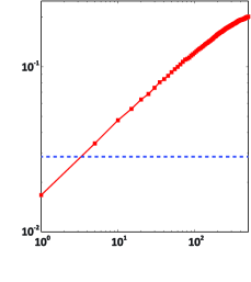
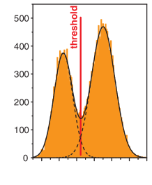
In conventional readout, the fast ns repolarization of the NV electronic spin limits the number of photons an NV emits before all initial spin state information is lost (see Fig. 6). Even when implementing conventional readout with the best present collection efficiencies, the average number of collected photons per NV center is less than 1, and for many implementations , making photon shot noise the dominant contributor to the parameter (see Eqn. 12, Table 2, Sec. V.5). An alternative method to increase the readout fidelity circumvents this problem by instead first mapping the initial NV electronic spin state information onto an ancilla nuclear spin. In the second step, the ancilla nuclear spin state is mapped back onto the electron spin, which is then detected using conventional fluorescence-based readout. This second step may be repeated many times with each marginal readout improving the aggregate readout fidelity, as shown in Fig. 23a,b. While first demonstrated with a nearby 13C nuclear spin as the ancilla Jiang et al. (2009), the technique was later realized using the NV center’s 14N Neumann et al. (2010a) and 15N nuclear spin Lovchinsky et al. (2016). In the realization Jiang et al. (2009); Maurer et al. (2012), the coupling to the ancilla spin depends on the distance between the NV defect and the nearby atom, making the technique difficult to implement for NV ensembles where this distance varies. This discussion instead focuses on the more scalable realization using the NV nitrogen nuclear spin as the ancilla, which ensures the electron spin to ancilla spin coupling remains fixed over the NV ensemble.
Figure 23c shows a quantum circuit diagram from Ref. Lovchinsky et al. (2016) depicting the repetitive readout scheme. After the final MW pulse in an NV sensing protocol, the NV electronic spin state (denoted by subscript ) is mapped onto the nitrogen nuclear spin state (subscript ). In Ref. Lovchinsky et al. (2016), this mapping is achieved using a SWAP gate (), where CNOT denotes a controlled NOT gate. The SWAP gate consists of a MW -pulse, then an RF -pulse, then another MW -pulse, where the MW pulses flip the electronic spin and the RF pulse flips the nuclear spin. This procedure swaps the electronic and nuclear spin states, importantly, storing the electronic spin state information in the ancilla nuclear spin. Then an optical pulse re-polarizes the electronic spin to . Next, a set of repetitive readouts is performed. In each readout, the nuclear spin state is copied back onto the electronic spin with a MW pulse, (a gate), and then the electronic spin is optically read out without affecting the nuclear spin state. This process can be repeated many times (), and is limited in principle by the nuclear spin lifetime . In Ref. Lovchinsky et al. (2016), while the initial RF pulse used in the SWAP gate requires 50-60 s, each readout cycle requires only s. The large number of readouts allow the aggregate readout fidelity to approach 1; notably, Ref. Neumann et al. (2010a) achieves as depicted in Fig. 23b.
Extending ancilla-assisted repetitive readout to ensembles is expected to be fruitful but necessitates overcoming further challenges. The scheme requires a large magnetic field to minimize coupling between the NV nuclear and electronic spins, with Refs. Neumann et al. (2010a); Lovchinsky et al. (2016) employing fields of 2500 gauss and 6500 gauss respectively. Further, the bias magnetic field must be precisely aligned along a single NV symmetry axis, presently precluding its use for sensing from more than one NV orientation Schloss et al. (2018). Even slight angular misalignments introduce measurement back action on the nuclear spin , which spoils Neumann et al. (2010a). The reduction in limits the available readout duration. Ensemble implementations would therefore require highly uniform bias magnetic fields over ensemble sensing volumes, conceivably on the scale. Engineering such fields is within current technical capability but difficult nevertheless (see Sec. III.3 and Ref. Vandersypen and Chuang (2005)). Additionally, the MW and RF control pulses would ideally manipulate the entire ensemble uniformly; spatial inhomogeneities of the control pulses are likely to result in reduced readout fidelity unless mitigated Vandersypen and Chuang (2005). Assuming sufficiently strong and homogeneous fields and MW driving can be realized, and that the additional overhead time is acceptable, repetitive readout appears to be a promising but technically demanding method to improve for ensembles.
V.4 Level-anticrossing-assisted readout
In conventional readout Doherty et al. (2013), the readout fidelity depends on the number of photons collected per measurement sequence (see Eqn. 12). The value of is limited by the time the spin population originally in the states spends shelved in the singlet state before decaying to the triplet state. Steiner et al. engineer the NV spin to pass through the singlet state multiple times before repolarization, extending the readout duration per sequence to increase Steiner et al. (2010), as depicted in Fig. 24. Using NV centers with 14N, which has nuclear spin , three cycles through the singlet state occur during readout, yielding a increase in and thus a improvement in the fidelity . For NV centers with with , the spin only passes twice through the singlet state before repolarization, yielding only a improvement in .
The technique is implemented as follows: the bias field is tuned to the excited-state level anticrossing at G Fuchs et al. (2008); Neumann et al. (2010a) to allow resonant flip-flops between the NV center’s electronic spin and its 14N nuclear spin (). Operation at the level anticrossing polarizes the nuclear spin into the state Jacques et al. (2009). At completion of a sensing sequence, immediately prior to readout, the NV electronic spin occupies a superposition of the states and . Before the NV electronic spin state is read out using a conventional green laser pulse, two sequential RF -pulses flip the nuclear spin into the state, conditional on the electronic spin occupying the state. This CNOT gate relies on the RF drive being resonant with the nuclear transitions between the states for population in the state and off-resonant for population in the state. During readout, the population in cycles through the long-lived singlet state three times before the information stored in the NV electronic spin is lost, allowing more signal photons to be collected. After the first and second pass through the singlet to the state, an electron-nuclear spin flip-flop returns the electronic spin state to , as shown in Fig. 3a of Ref. Steiner et al. (2010), enabling another cycle through the singlet state. The third pass repolarizes the NV spin into the stable state.
This technique’s utility for magnetic sensing depends on whether the increase in fidelity outweighs the cost of additional overhead time (see Eqn. 10) introduced by the RF pulses. Although the authors of Ref. Steiner et al. (2010) assert that microsecond-scale RF nuclear spin -pulses are attainable, achieving such nuclear Rabi frequencies over large ensemble volumes may prove very difficult, making this method impractical for NV ensembles with s. Additional challenges for implementation with NV ensembles include realizing the requisite uniformity in the MW/RF fields and in the 500 G bias magnetic field over ensemble volumes. Finally, the scheme presently precludes sensing from more than one NV orientation Schloss et al. (2018).
V.5 Improved photon collection methods
In the limit of low contrast, the readout fidelity is proportional to the square root of the average number of photons collected per NV per measurement, i.e., (see Eqn. 12). Under these conditions, sensitivity can be enhanced by increasing the geometric collection efficiency , defined as , where and are the number of photons collected and emitted respectively by the NV ensemble per measurement.
Efficient photon collection in diamond is hindered by total-internal-reflection confinement resulting from diamond’s high refractive index of approximately 2.41. For example, air and oil immersion objectives, with numerical apertures of 0.95 and 1.49 respectively, provide calculated collection efficiencies of only and respectively for photons emitted directly through the {100} diamond surface Le Sage et al. (2012), as depicted in Fig. 25. Although anti-reflection coatings can allow for higher collection efficiencies, present implementations demonstrate only modest improvement Yeung et al. (2012). While great effort has resulted in high values of for single NV centers through use of various nano-fabrication approaches Hadden et al. (2010); Babinec et al. (2010); Marseglia et al. (2011); Choy et al. (2011); Schröder et al. (2011); Yeung et al. (2012); Choy et al. (2013); Riedel et al. (2014); Neu et al. (2014); Momenzadeh et al. (2015); Li et al. (2015); Shields et al. (2015); Häberle et al. (2017), such methods do not easily translate to large ensembles.
Successful approaches for bulk ensemble magnetometers have so far focused on collecting NV fluorescence that has undergone total internal reflection in the diamond Le Sage et al. (2012); Wolf et al. (2015b). While absorption of NV fluorescence by various defects may limit Khan et al. (2013, 2009) for some diamonds, nitrogen Weerdt and Collins (2008) and NV centers Fraczek et al. (2017) are expected to hardly absorb in the NV PL band nm. A collection efficiency of 39 is demonstrated in Ref. Le Sage et al. (2012) by detecting fluorescence from the four sides of a rectangular diamond chip surrounded by four photodiodes (see Fig. 26). However, the increased experimental complexity associated with employing four detectors in contact with the diamond may be problematic for certain applications. In another approach, Wolf et al. employ a trapezoidally-cut diamond chip and a parabolic concentrator to improve collection efficiency Wolf et al. (2015b). Although the authors calculate to be between and , this result is not confirmed experimentally. Ma et al. Ma et al. (2018) demonstrate a collection efficiency of 40 by eliminating all air interfaces between the diamond and detector, in conjunction with coupling prisms which direct light exiting the diamond’s four side faces to the detector.
In the future, collection efficiency in bulk NV-diamond magnetometers is expected to improve to near 100, limited only by losses due to absorption. For example, light lost from the top and sides of the diamond in Ref. Wolf et al. (2015b) could be redirected to the detector by coating these sides of the diamond with a metallic Choy et al. (2011) or dielectric reflector Boesch et al. (2016). The authors of Ref. Wolf et al. (2015b) might also see an improvement in collection efficiency by designing an optimized parabolic concentrator rather than using a commercially available part. Hypothetical geometries for light collection using parabolic or ellipsoidal reflectors are discussed in Ref. Boesch et al. (2016). Whereas multiple-reflection methods are suitable for bulk magnetometers, increasing by collecting light undergoing multiple reflections in the diamond may substantially complicate accurate image reconstruction for NV magnetic imaging microscopes Steiner et al. (2010); Pham et al. (2011); Le Sage et al. (2013).
Is is also natural to consider exploiting the Purcell effect to improve readout fidelity. By engineering physical structures around a chosen NV center or ensemble, several works have increased the triplet excited state’s radiative decay rate Kaupp et al. (2016); Choy et al. (2011); Riedel et al. (2017). The increased radiative decay allows for more PL photons to be collected from population originally in while population originally in is shelved in the singlet states. Although theoretical investigations suggest that Purcell enhancement might improve readout fidelity Wolf et al. (2015a) or leave fidelity unchanged Babinec et al. (2012), the only reported experimental demonstration of Purcell-enhanced NV spin readout to date finds reduced fidelity Bogdanov et al. (2017). The authors surmise that charge effects related to dense NV ensembles may contribute to the observed fidelity decrease. Achieving high Purcell factors for NV ensemble applications may also impose undesirable geometric constraints. For a clear and detailed discussion of radiative lifetime engineering for NV spin readout, we recommend Ref. Hopper et al. (2018b). Along similar lines, a recent proposal suggests that NIR fluorescence-based readout could exhibit improved fidelity over conventional readout when combined with Purcell enhancement Meirzada et al. (2019). While this scheme requires high IR excitation intensities likely incompatible with large NV ensembles, it may show utility for small ensembles within a confocal volume.
V.6 Near-infrared absorption readout
The sensitivity of conventional fluorescence-based readout is limited by shot noise on the collected photons due to low fluorescence contrast (see Eqn. 11). As an alternative to fluorescence-based readout, population in one or both NV singlet states may be directly probed via absorption, giving a probabilistic measure of the initial spin state prior to readout. While the upper singlet state 1A1 lifetime ns at room temperature Acosta et al. (2010b); Ulbricht and Loh (2018) is likely too short for such an approach to be effective, the lower singlet state 1E lifetime ns at room temperature Gupta et al. (2016); Robledo et al. (2011); Acosta et al. (2010b) makes measuring the 1E population via absorption on the 1E transition at 1042 nm viable.
Near-infrared (NIR) absorption has attractive benefits for certain applications: a) Contrast (and therefore sensitivity) is not reduced by background fluorescence from non-NV defects (such as NV0). b) The directional nature of the 1042 nm probe light allows maximal collection efficiency (ignoring absorptive losses) to be obtained more easily than in a fluorescence-based measurement; for example, this benefit was exploited in the first demonstration of microwave-free magnetometry with NV centers Wickenbrock et al. (2016). c) Owing to the upper singlet 1A1 lifetime of ns Acosta et al. (2010b); Ulbricht and Loh (2018), the saturation intensity of the 1E transition is unusually large ( megawatts/cm2 Dumeige et al. (2013)), allowing high intensity 1042 nm probe radiation to be used, so that fractional shot noise is reduced to well below that of an equivalent fluorescence-based measurement Acosta (2011). d) NIR absorption readout is nondestructive, allowing for a single NV center in the 1E singlet state to absorb multiple 1042 nm photons before eventual decay to the 3A2 triplet. In principle such absorption by a single NV center can allow readout fidelity near the spin-projection limit, even in the presence of non-negligible optical losses.
NIR absorption readout has been successfully implemented in several proof-of-principle magnetometers. In the first demonstration Acosta et al. (2010), a diamond containing ppm is continuously illuminated with 532 nm radiation (driving the 3AE transition to optically polarize the NV spin state) and 1042 nm NIR radiation (resonantly addressing the 1E transition), as shown in Fig. 27a. MW radiation transfers population between the ground state Zeeman sublevels. In this first demonstration Acosta et al. (2010), a single pass of the 1042 nm radiation through the diamond sample resulted in a peak-to-peak contrast of at room temperature.
The contrast can be enhanced by increasing the number of NV defects interacting with each 1042 nm photon, such as by employing a higher NV density or a larger diamond. Alternatively, for a fixed number of NV centers, the 1042 nm radiation can be recirculated through the diamond. An NIR absorption magnetometer employing an optical cavity to increase the 1042 nm interaction length is analyzed in Ref. Dumeige et al. (2013) and experimentally realizes a peak-to-peak contrast of in Ref. Jensen et al. (2014) when the bias magnetic field is directed along the [100] crystallographic direction (making the magnetic resonances of all four NV orientations degenerate). For this demonstration, the diamond is anti-reflection coated Yeung et al. (2012) and placed in the center of a dual-wavelength optical cavity, which allows recirculation of both 1042 nm and 532 nm radiation. The more efficient use of the 532 nm light enabled by the cavity allows both a larger NV ensemble to be addressed and a higher degree of spin initialization into the state. Ultimately the device in Ref. Jensen et al. (2014) achieves a sensitivity of 2.5 nT/, well above the shot-noise limit of 70 pT/.
A notable recent implementation of NIR absorption Chatzidrosos et al. (2017) is depicted in Fig. 27b. One diamond face forms a reflector while the addition of a dual-wavelength concave mirror results in an optical cavity with a finesse of 160 and a cylindrical sensing volume of m diameter and m length Chatzidrosos et al. (2017). With 500 mW of 532 nm radiation and 80 mW of 1042 nm radiation, a DC magnetic field sensitivity of 28 pT/ is achieved with this compact setup, with a bandwidth of about 530 Hz. The shot-noise-limited sensitivity is 22 pT/ and the spin-projection-noise-limited sensitivity is 0.43 pT/.
The NIR absorption approach is hindered, however, by several non-idealities, which so far limit readout fidelity to values far from the spin projection noise limit, similar to conventional optical readout (i.e., for the NIR absorption approach in Ref. Chatzidrosos et al. (2017) versus for conventional readout in Ref. Le Sage et al. (2012)). First, the predominantly non-radiative decay of the 1A1 singlet greatly reduces the absorption cross section of the 1E transition compared to a radiative-decay-only transition Rogers et al. (2008); Acosta et al. (2010b). Estimates suggest cm2 Kehayias et al. (2013); Dumeige et al. (2013); Jensen et al. (2014), whereas the purely radiative 3AE transition is measured to have a much larger absorption cross section cm2 for 532 nm excitation, as shown in Table 17. Realizing the full potential of this method requires 1042 nm laser intensities of order MW/cm2 Jensen et al. (2014). This saturation intensity appears to limit interrogation cross sections to m2 for mW-scale 1042 nm radiation powers, assuming a cavity finesse of . Laser intensities of this magnitude may lead to undesirable ionization dynamics (see Sec. VI.2). We note that many absorption cross section measurements neglect ionization/recombination dynamics, which may skew reported values Meirzada et al. (2018, 2019). Second, as described in Ref. Dumeige et al. (2013), non-resonant losses for 1042 nm radiation compromise sensitivity by reducing the effective achievable collection efficiency. For example, in Ref. Chatzidrosos et al. (2017), 80 mW of 1042 nm radiation input to the dual-wavelength cavity results in 4.2 mW transmitted to the detector. Third, the NIR absorption has only been demonstrated for dense ensembles with ppm to ensure appreciable 1042 nm absorption; the performance of this method for diamonds with more dilute NV concentrations and longer values remains unknown, and will likely depend on the scaling of cavity finesse with [N] or [NV] density.
While NIR absorption readout is effective and may find preference for certain applications Wickenbrock et al. (2016); Chatzidrosos et al. (2017), without further advances enabling readout fidelity enhancement, (e.g., reduced 1042 nm non-resonant absorption or reduced non-radiative 1A1 singlet decay rate), this method will remain approximately on par with conventional fluorescence readout while requiring the non-trivial overhead of an NIR single frequency laser and an optical cavity.
V.7 Green absorption readout
Alternatively, NV readout may be achieved by monitoring absorption of green probe laser radiation, which off-resonantly drives the triplet 3AE transition Bauch (2010); Walsworth (2017). When resonant MWs drive the or ground state spin transitions and facilitate population transfer to the NV singlet states, it is expected that the 3A2 state will be depleted, resulting in increased green probe transmission and decreased red fluorescence. For absorption measurements (both NIR and green), the change in transmitted light upon resonant MW drive is expected to mirror the change in fluorescence light up to a scaling constant, since transmission is minimal when fluorescence is maximal and vice versa Bauch (2010). Data consistent with this understanding is shown in Fig. 28 for NV centers illuminated with 514 nm light.
The absorption contrast, denoted , may differ substantially in magnitude from the fluorescence contrast (see Fig. 28). Because absorption measurements monitor transmitted light, the detected signal (and thus ) depends on the optical depth of the absorbing material. For example, even for the idealized case where , if only a small fraction of the incident light is absorbed in the absence of MWs, the change in transmission upon application of resonant MWs will necessarily also be small, yielding a low absorption contrast . Additionally, the absorption contrast may be further decreased due to the presence of non-radiative decay pathways.
Observed magnitudes of in the literature are lower than by Bauch (2010); Le Sage and Arai (2011) or more. For example, the authors of Refs. Ahmadi et al. (2017, 2018b, 2018a) use a CW-ODMR-based magnetometer employing a resonant optical cavity to recycle the green excitation light through the diamond multiple times, and observe , (which is typical), while measuring . In Ref. Ahmadi et al. (2018a) the same experimental setup performs magnetometry simultaneously using both green absorption and red fluorescence, as shown in Fig. 29. The green absorption yields sensitivity while the conventional readout based on red fluorescence reaches , about 250 better. As with NIR absorption readout (see Sec. V.6), recycling the green excitation light via a resonant optical cavity can increase the absorption signal by (i) addressing a larger NV population, (ii) improving initialization into the state, or (iii) enhancing . Although effectively implemented absorption readout may achieve higher optical collection efficiency than fluorescence detection, the low realized absorption contrasts are a current major drawback.
Furthermore, absorption behavior for 532 nm probe radiation can result in increased probe laser transmission under resonant MW application Bauch (2010); Le Sage and Arai (2011), leading to an anomalous inversion of the green absorption signal. This deviation from expected behavior has been independently observed in multiple research groups Bauch (2010); Le Sage and Arai (2011). The anomalous reveals a strong wavelength and power dependence Bauch (2010), which suggests that green absorption readout is hindered by an unknown effect competing with and sometimes dominating otherwise expected behavior. The wavelength and power dependence of this effect suggests NV0/NV charge dynamics could play a role. Further investigation of this behavior might reveal presently unknown NV dynamics. Overall, given the low absorption contrast , and yet unknown mechanism of anomalous absorption behavior, the utility of green absorption readout remains questionable.
V.8 Laser threshold magnetometry
Another approach for bulk NV magnetometry is the creation of a NV-diamond-based laser threshold magnetometer, as suggested by Ref. Jeske et al. (2016). Lasing is induced on the NV transition; then, when a magnetic-field-dependent population accumulates in the singlet state, the lasing threshold increases, and the laser’s output power is reduced. As theoretically outlined Jeske et al. (2017); Savitski (2017), the laser threshold approach has a number of benefits relative to generic CW-ODMR methods (Sec. II.2.1): (i), effective contrast is enhanced near the lasing threshold due to competition between stimulated and spontaneous emission, (ii) collection efficiency is substantially improved by virtue of the lasing process. Although the emission cross sections for NV and NV0 have been measured Fraczek et al. (2017), and stimulated emission from NV was recently demonstrated Jeske et al. (2017), substantial work remains to address potential problems. For example, absorption by substitutional nitrogen or other defects may obstruct the lasing process Dodson et al. (2011), and it will need to be shown that other sources of noise affecting the lasing threshold or output power can be either controlled or normalized out Jeske et al. (2016). More concerning, however, is that both theory DeGiorgio and Scully (1970) and experiment Lim et al. (2002) find large laser field fluctuations in the vicinity of the lasing threshold.
VI Diamond material engineering
VI.1 Conversion efficiency
In an idealized case in which all other parameters are held constant, increasing the NV density in a fixed detection volume will result in enhanced sensitivity. Since the NV density is limited by the density of nitrogen introduced into the diamond, the N-to-NV conversion efficiency
| (31) |
must be increased in order to achieve a high density of NV spins while minimizing the concentration of residual paramagnetic substitutional nitrogen. Converting a substitutional nitrogen N into a NV defect requires both introducing a vacancy to a lattice site adjacent to a substitutional nitrogen (to create the NV), and capturing an electron (to change the NV center’s charge state to NV). We denote the efficiency with which nitrogen atoms in the diamond are converted to NVs as
| (32) |
where accounts for the concentration of substitutional nitrogen N in the neutral and ionized charge states, NV centers in all three charge states, and other nitrogen-containing defects in the diamond, such as NVH (see Sec. VI.6). We define the fraction of NV centers residing in the negative charge state as the charge state efficiency ,
| (33) |
so that . Although Refs. Pfender et al. (2017); Hauf et al. (2014) show evidence for NV+, this state has so far required application of external voltages for observation. The rest of this section therefore assumes [NV+] is negligible and can be ignored.
As the N-to-NV conversion efficiency is determined by the physical location of nitrogen and vacancies in the diamond lattice, the value of is expected to be invariant under ambient conditions. Modification of requires conditions severe enough to rearrange atoms within the diamond lattice, such as irradiation, implantation, high temperature, or high pressure. With suitable electron irradiation and subsequent annealing, N-to-NV conversion efficiencies approaching 1 can be achieved, although such high values are not necessarily desirable (see Secs. VI.4 and VI.5).
In contrast, the charge state efficiency depends on local conditions in the diamond and can be affected by external fields and optical illumination. Increasing benefits sensitivity in two ways: first, by increasing the NV concentration and thus the number of collected photons from the NV ensemble; and second, by decreasing the concentration of NV and the associated background fluorescence, which improves measurement contrast. In the following section we discuss factors contributing to the charge state efficiency and methods to optimize it for sensing.
VI.2 NV charge state efficiency
The charge state efficiency from Eqn. 33, depends on many factors both internal and external to the diamond. For both native NVs Iakoubovskii et al. (2000) and NVs created by irradiation and annealing of nitrogen-rich diamonds Mita (1996), the NV and NV0 charge states can coexist in a single sample. In general, for a given sample and experimental procedure, the steady-state charge state efficiency is difficult to predict. Contributing factors include the concentration of substitutional nitrogen and other defects serving as charge donors or acceptors Groot-Berning et al. (2014) and their microscopic distributions Collins (2002); Doi et al. (2016); the wavelength, intensity, and duty cycle of optical illumination Doi et al. (2016); Manson and Harrison (2005); Aslam et al. (2013); Ji and Dutt (2016); the application of a bias voltage Grotz et al. (2012); Kato et al. (2013); Schreyvogel et al. (2014); Doi et al. (2014); and, for near-surface NVs, the diamond surface termination Rondin et al. (2010); Fu et al. (2010); Hauf et al. (2011); Cui and Hu (2013); Groot-Berning et al. (2014); Chu et al. (2014); Yamano et al. (2017); Kageura et al. (2017); Osterkamp et al. (2015); Newell et al. (2016); Santori et al. (2009). The charge state efficiency is likely affected by the conditions of diamond growth, as well as the irradiation dose Mita (1996) (see Sec. VI.4), the annealing duration and temperature, and possibly the operation temperature Manson and Harrison (2005). Moreover, the value of the charge state efficiency during an NV sensing procedure can be difficult to measure. NVs may be reversibly converted between NV and NV0 by various optical and non-optical processes Khan et al. (2009); Aslam et al. (2013); Bourgeois et al. (2017). Because is strongly affected by the illumination laser intensity and wavelength Aslam et al. (2013); Bourgeois et al. (2017), characterization of by methods such as Fourier-transform infrared spectroscopy (FTIR), ultraviolet-visible (UV-Vis) spectroscopy, and electron paramagnetic resonance (EPR) may be misrepresentative of NV charge state behavior under the optical illumination employed in most NV-diamond sensing devices.
VI.2.1 Non-optical effects on NV charge state efficiency
Here we discuss the charge state efficiency in nitrogen-rich diamond in the absence of optical illumination. For shallow NVs, the charge state is strongly affected by the surface chemical termination Rondin et al. (2010); Fu et al. (2010); Hauf et al. (2011); Cui and Hu (2013); Groot-Berning et al. (2014). Based on the work in Ref. Groot-Berning et al. (2014), surface termination should provide enhanced charge state stability to a depth of at least 60 nm and possibly farther Santori et al. (2009); Malinauskas et al. (2008). The charge state efficiency can also be controlled electrically Grotz et al. (2012); Kato et al. (2013); Schreyvogel et al. (2014); Doi et al. (2014); Schreyvogel et al. (2015); Hauf et al. (2014); Murai et al. (2018); Forneris et al. (2017); Karaveli et al. (2016). Because diamond is an approximately 5.47 eV wide band gap insulator Wort and Balmer (2008), Ref. Collins (2002) contends that an NV center’s charge state depends less on the position of the Fermi level and more on the distance to the nearest charge donor. In nitrogen-rich diamonds, these donors are mainly substitutional nitrogen defects N, and the charge state efficiency is seen to increase with the concentration Collins (2002); Manson and Harrison (2005). Other defects in the diamond lattice can alter as well; for example, in Ref. Groot-Berning et al. (2014), the NVs in separate implanted regions containing phosphorus (an electron donor) and boron (an electron acceptor), were seen to have increased, and respectively decreased, NV charge state efficiencies.
Introduction of electron donors other than nitrogen into diamond might appear to be a promising avenue for increasing the NV charge state efficiency. For example, phosphorus Groot-Berning et al. (2014); Doi et al. (2016); Murai et al. (2018), with donor level 0.6 eV below the conduction band Katagiri et al. (2004), is a shallower donor than nitrogen, which lies 1.7 eV below the conduction band Farrer (1969); Wort and Balmer (2008). However, creating n-doped diamond through introduction of phosphorus has proven difficult Kalish (1999), as phosphorus doping is correlated with the introduction of a deep acceptor tentatively identified as the phosphorus vacancy (PV) Jones et al. (1996). Moreover, irradiation and annealing to create NV centers may further convert desirable substitutional phosphorus into PVs Jones et al. (1996). PVs in diamond will compete with NVs for electrons, undermining the benefit of phosphor doping to the charge state efficiency. Additionally, PL emission at wavelengths overlapping the NV PL spectrum was observed in phosphorus-doped diamond Cao et al. (1995), further complicating the use of phosphorus in NV-diamond sensing. For additional discussion see Ref. Doherty et al. (2016).
The irradiation and annealing procedures applied to increase the N-to-NV conversion efficiency can also affect the charge state efficiency . In Type Ib diamonds grown by high-pressure-high-temperature (HPHT) synthesis (see Sec. VI.3), with ppm, approaching 1 is seen after low- and moderate-dose irradiation and annealing Manson and Harrison (2005); Mita (1996). As discussed in Sec. VI.4, at higher irradiation doses, the NV0 concentration is seen to abruptly increase Mita (1996), which can be attributed to the combination of an insufficient concentration of nitrogen defects N available to donate electrons to the increasing overall NV population, and an increase in deep acceptor states such as multi-vacancy defects Twitchen et al. (1999b); Pu et al. (2001).
VI.2.2 Optical effects on NV charge state efficiency
Optical illumination of diamond may also change the NV charge state efficiency through ionization of NV to NV0 and also recombination of NV0 back to NV Manson and Harrison (2005); Aslam et al. (2013); Waldherr et al. (2011); Hopper et al. (2016, 2018a). The steady-state value of is seen to depend on the illumination intensity and wavelength, although most of the reported measurements have been taken on single NV centers Aslam et al. (2013); Waldherr et al. (2011); Hopper et al. (2016). For example, an excitation wavelength band from 510 nm to 540 nm was found to produce the most favorable single-NV charge state efficiency in steady state compared to longer and shorter wavelengths Aslam et al. (2013). In particular, when single NVs were illuminated by 532 nm light at intensities typical for pulsed sensing protocols Hopper et al. (2016); Waldherr et al. (2011) or similar wavelength light at lower intensities Aslam et al. (2013), a charge state efficiency was observed. However, the value of under these conditions is likely to differ for dense NV ensembles Manson and Harrison (2005); Meirzada et al. (2018). For example, measurements in Ref. Manson and Harrison (2005) on an NV ensemble in a diamond with ppm and ppm show the charge state efficiency dropping to as the 532 nm power approaches the saturation power of the NV optical transition. More study is required to determine the relative contributions to the NV ensemble of optical charge-state switching, the presence of nearby charge donors/acceptors, and other effects.
Recently, several studies on single NV centers have shown improved optical initialization to NV by applying near-infrared radiation (NIR) in combination with the 532 nm green excitation light Hopper et al. (2016); Ji and Dutt (2016); Chen et al. (2017). This enhanced charge-state initialization has been demonstrated with 780 nm CW radiation Chen et al. (2017), 1064 nm CW radiation Ji and Dutt (2016), and 900 nm - 1000 nm pulsed radiation, achieving in the third case Hopper et al. (2016). The effect is theoretically explained as follows: after absorption of a green photon to enter the electronically excited state, an NV0 absorbs an NIR photon, which promotes a hole to the valence band and forms NV Ji and Dutt (2016); Hopper et al. (2016). The mechanism, visualized schematically in Fig. 30, is the same as the two-photon ionization and recombination of NV and NV0 by 532 nm radiation, but with the second absorbed photon being an NIR photon. In Ref. Hopper et al. (2016) the NV0-to-NV recombination process is found to occur with up to a higher likelihood than the analogous ionization process converting NV to NV0, wherein the excited-state NV absorbs an NIR photon, promoting an electron to the conduction band.
NIR-enhancement of charge state efficiency is expected to be compatible with pulsed initialization and readout. However, when employing 532 nm intensities mW/m2 Wee et al. (2007) typical for pulsed experiments, Ref. Hopper et al. (2016) finds enhancements in to be lessened compared to operation at lower green intensity. Furthermore, if the charge switching rate under green-plus-NIR illumination approaches or exceeds the optical spin polarization rate, spin readout fidelity could be degraded by the increased photoionization during the readout pulse. Refs. Ji and Dutt (2016) and Chen et al. (2017) report charge switching rates near , approaching the singlet state decay rate of Acosta et al. (2010b). Nonetheless, Hopper et al. achieve enhanced charge state initialization with much lower charge switching rates of ms.
Further work is required to determine if the NIR-plus-green illumination technique can be extended to increase the charge state efficiency in NV ensembles. While the technique has shown success for near-surface NV centers, Ref. Meirzada et al. (2018) observes no enhancement in the NV PL from NIR-plus-green illumination compared to green-only excitation for NV centers in bulk diamond. Moreover, even if NIR-plus-green illumination can enhance the ensemble value of , the power requirements may limit the technique’s application to large ensembles. Although the required NIR power for confocal setups addressing single NV centers or small ensembles is modest ( mW), the NIR intensity is higher than the typical 532 nm intensities used for NV spin initialization ( in Ref. Hopper et al. (2016)). Thus, when applying the technique to macroscopic ensemble volumes, the maximum addressable ensemble size will quickly be limited by the available laser power. For example, a spot would require W of NIR Wee et al. (2007). At present, NIR-enhancement of charge state efficiency appears unlikely to yield substantial improvements to ensemble-NV magnetometer sensitivities.
VI.3 Diamond synthesis and high pressure high temperature treatment
Fabricated bulk diamonds are commonly synthesized using one of two methods. In high pressure high temperature (HPHT) synthesis, a process mimicking natural diamond formation, a carbon source material is mechanically compressed (pressure > 5 GPa) and heated (temperatures ∘C) to create conditions where diamond is the thermodynamically favored carbon allotrope. Dissolving the carbon source (typically graphite) in a metal "solvent-catalyst" can increase the growth rate, decrease the required temperature and pressure, and allow for better composition control. Consequently, solvent-catalysts are nearly always employed. A small seed diamond facilitates the growth; the dissolved carbon precipitates out of the metal catalyst solution and crystallizes onto the seed diamond, growing the size. Nitrogen easily incorporates into the diamond lattice, and is historically the primary impurity element in HPHT diamonds. However, nitrogen content in HPHT-synthesized diamonds can be reduced by varying the atomic composition of the metal solvent catalyst to “getter” the nitrogen, and recent advances in getter technology have allowed direct creation of electronic grade HPHT diamond with [N] 5 ppb D’Haenens-Johansson et al. (2015); Tallaire et al. (2017b). References Kanda (2000); Dobrinets et al. (2013); Palyanov et al. (2015) discuss HPHT synthesis in detail.
Plasma-enhanced chemical vapor deposition (PE-CVD) diamond synthesis Angus et al. (1968) is a popular alternative to HPHT synthesis, and can leverage established semiconductor fabrication techniques. In the most widespread variant of this method, employing homo-epitaxial growth, a diamond seed is exposed to a hydrocarbon plasma consisting of approximately 95 - 99% hydrogen, with the balance composed of carbon and possibly other species such as oxygen or argon. Methane is the most popular carbon source. Radicalized carbon atoms bond with the growth surface, forming a mixture of sp2 and sp3 bonded orbitals. Although hydrogen etches both sp2 and sp3 bonded carbon, the etch rate for sp2 bonded carbon is much greater Schwander and Partes (2011) and, if the hydrogen etching and carbon deposition rates are carefully tuned, diamond synthesis can be achieved Angus et al. (1968). Unlike HPHT synthesis, PE-CVD (alternatively simply called CVD) synthesis can easily allow the production of thin or delta doped layers from nanometer to micron scale Ohno et al. (2012); McLellan et al. (2016), masked synthesis of diamond structures Zhang and Hu (2016), or layered epitaxial growth required for PIN Kato et al. (2013) or NIN structures Murai et al. (2018).
In the past 15 years, the majority of NV-diamond literature has employed diamonds grown by PE-CVD. First, much early work focused on single NV centers; and most HPHT-synthesized diamonds were not available at that time with the requisite low nitrogen concentration ( 100 ppb), as HPHT impurity control can be challenging Martineau et al. (2009); Gaukroger et al. (2008). Second, the layered deposition inherent to CVD allows straightforward growth of epitaxial layers (as would be required for magnetic imaging devices) and the application of semi-conductor techniques to control diamond composition. Third, the PE-CVD method was historically more popular with commercial collaborators (such as Element Six and Apollo Diamond) responsible for producing the majority of scientific diamonds containing NV centers.
In addition, several challenges accompany direct HPHT synthesis of high-quality NV-diamonds. For one, solvent-catalyst incorporation into the diamond lattice may result in metal inclusions with size visible to the naked eye. Such inclusions could be particularly problematic for magnetic sensing applications, since the common materials employed in the solvent catalyst alloys are the ferromagnetic elements Fe, Co, and Ni Palyanov et al. (2015). The purity of HPHT-synthesized diamonds may be limited by the solid precursor materials, which may not be available with as high chemical or isotopic purity as the gas-phase precursor elements employed for CVD synthesis. Finally, the HPHT process is not intrinsically amenable to fabrication of NV-rich layers, as are needed for imaging applications. In spite of these challenges, HPHT-fabricated diamonds with good characteristics for ensemble-NV DC magnetometry - including long (s), high (), and [N 1-4 ppm - have been recently reported in the literature Wolf et al. (2015b); Grezes et al. (2015); Stürner et al. (2019) (see Table 6).
| Reference | E | [NV] | [NV0] | [N] | Synthesis | |||
|---|---|---|---|---|---|---|---|---|
| Grezes et al. (2015) | s | 84 s | 29 | 0.4 ppm | 0.4 ppm | 1.4 ppm | 300 ppm | HPHT |
| Wolf et al. (2015b) | - | s | 30 | 0.9 ppm | - | 3 ppm | - | HPHT |
| Zheng et al. (2019) | s | - | - | ppm | - | ppm | 300 ppm | HPHT |
| Hartland (2014) | - | - | 28 | ppm | 0.7 ppm | 4.1 ppm | 10700 ppm | CVD+HPHT |
| Schloss (2019) | s | s | ppm | - | ppm | ppm | CVD | |
| Barry et al. (2016) | 580 ns | 5.1 s | 6.3 | ppm | - | 27 ppm | 10 ppm | CVD |
| Schloss et al. (2018) | 450 ns | s | ppm | ppm | ppm | 10700 ppm | CVD |
While the exact motivation for HPHT diamond synthesis is not always explicitly stated Teraji et al. (2013), HPHT synthesis may circumvent undesired characteristics inherent to CVD-synthesized diamonds Hartland (2014); Charles et al. (2004). A serious disadvantage of CVD synthesis is the incorporation of unwanted impurities and charge traps into the lattice (see Sec. VI.6). In addition, CVD-grown diamonds may display undesirable strain non-uniformities or contain a high dislocation density. For example, CVD-grown diamonds sometimes exhibit a brown coloration, which is attributed to vacancy cluster incorporation during synthesis Hounsome et al. (2006); Khan et al. (2013). As vacancy clusters, chains, and rings are typically paramagnetic Iakoubovskii and Stesmans (2002); Yamamoto et al. (2013b); Lomer and Wild (1973); Baker (2007), these clusters can increase NV ensemble dephasing, reducing . Additionally, since such vacancy chains and clusters are deeper electron acceptors than NV Khan et al. (2009); Edmonds et al. (2012), their presence may decrease measurement contrast Tallaire et al. (2017a). Naturally occurring diamond that has not undergone irradiation rarely contains vacancies Mainwood (1999), suggesting that vacancies and vacancy clusters should be uncommon in well-synthesized HPHT diamond. As point defects, dislocations, and other extended defects are believed to be the dominant sources of strain in Type IIa diamonds Fisher et al. (2006), HPHT-synthesized diamonds may also exhibit lower strain than their CVD-grown counterparts. While dislocation densities of cm are typical in CVD-grown diamonds Achard et al. (2014), certain HPHT-synthesized diamonds can demonstrate dislocation densities of cm Martineau et al. (2009); Tallaire et al. (2017b) and substantially lower strain D’Haenens-Johansson et al. (2014, 2015).
Although more research is needed, it is observed that the high quantity of hydrogen present during CVD growth can result in hydrogen incorporation into the diamond lattice Charles et al. (2004); Goss et al. (2014), (see Sec. VI.6). In contrast, diamonds synthesized directly by HPHT are unlikely to have hydrogen defects, as only one hydrogen-related defect has been found to incorporate into HPHT-synthesized diamond Hartland (2014).
Alternatively, mixed-synthesis approaches can combine the strengths of CVD and HPHT. One popular method is HPHT treatment, where an existing CVD diamond is heated and subjected to high pressure, resulting in atomic-scale reconfigurations of atoms in the lattice while leaving the macro-scale diamond largely unchanged Dobrinets et al. (2013). HPHT treatment effectively removes single vacancies Collins et al. (2000); Dobrinets et al. (2013) and causes vacancy clusters to dissociate Collins et al. (2000); Dobrinets et al. (2013) or aggregate Bangert et al. (2009). Thus, this method is effective to treat CVD-grown diamonds, which can exhibit vacancies and vacancy clusters Charles et al. (2004); Hartland (2014); Khan et al. (2013). The approach of applying HPHT treatment to CVD diamonds was proposed in Ref. Twitchen et al. (2010) and realized by the author of Ref. Hartland (2014), wherein a CVD-grown diamond was HPHT treated after synthesis but prior to irradiation and subsequent annealing (see Secs. VI.4 and VI.5). The diamond produced in Ref. Hartland (2014) exhibits a notably high 30 conversion efficiency = [NV]/[N] as shown in Table 10. A similar process pioneered by Lucent Diamonds employs HPHT treatment of diamonds prior to irradiation and annealing Vins (2007). This process results in a final material with an intense red hue and photoluminescence dominated by NV emission Wang et al. (2005); Dobrinets et al. (2013), suggesting that HPHT treatment can be effective to increase the charge state efficiency , likely by eliminating charge traps.
However, HPHT treatment cannot address all diamond deficiencies, CVD-related or otherwise. For example, should a CVD-synthesized diamond incorporate high concentrations of hydrogen or other elemental impurities into the diamond lattice during growth, HPHT treatment is ineffective to remove these impurities Charles et al. (2004). Such treatment is also limited to diamonds with balanced aspect ratios, as thin plates or rods will likely crack under the high applied pressure.
In addition to HPHT treatment of existing diamonds, other mixed-synthesis approaches have also been pursued. For example, utilizing type IIa HPHT seeds for CVD growth rather than CVD-grown seeds can yield material with lower strain and reduced densities of dislocations and other unwanted defects Martineau et al. (2009); Tallaire et al. (2017b); Gaukroger et al. (2008); Hoa et al. (2014). Another mixed-synthesis method exploits the fine composition control and high chemical purities available with CVD synthesis to create the carbon precursor for HPHT synthesis Teraji et al. (2013). The diamond composition can thus be carefully controlled, and HPHT synthesis can take advantage of high-purity or isotopically enriched gaseous sources (e.g., methane or 15N2).
Given the prominent role lattice defects and elemental impurities play in determining the charge state efficiency and coherence times for NV, additional research focused on synthesizing sensing-optimized diamonds is warranted.
VI.4 Electron irradiation
| N | Growth location | Reference | |
|---|---|---|---|
| ppm | Element Six | Edmonds et al. (2012) | |
| ppm | Apollo Diamond Inc. | Edmonds et al. (2012) | |
| ppm | Warwick University | Hartland (2014) |
| Reference | |
|---|---|
| ppb | Rutledge and Gleason (1998) |
| ppb | Twitchen et al. (2010) |
| ppb | Mainwood (1999) |
For unmodified as-grown CVD diamond, realized conversion efficiency values can be far less than unity, as shown in Table 7, where the majority of substitutional nitrogen is not converted to NV Edmonds et al. (2012); Hartland (2014). In fact, for some CVD diamonds (see Table 8) the concentration of grown-in monovacancies is insufficient to achieve good for total nitrogen concentration 1 ppm regardless of location; even if every monovacancy were adjacent to a substitutional nitrogen, the conversion efficiency would still be low Mainwood (1999); Deák et al. (2014). However, the monovacancy concentration can be augmented after growth by irradiating the diamond with energetic particles. The high-energy irradiating particles knock carbon atoms out of the diamond lattice, creating both interstitial carbon atoms and monovacancies Twitchen et al. (1999a); Newton et al. (2002). Although theoretical calculations have not yet completely converged with experimental observations Deák et al. (2014); Zaitsev et al. (2017), the widely accepted model posits that upon subsequent annealing (discussed in Sec. VI.5), diffusing vacancies are captured by substitutional nitrogen atoms, forming NV centers Acosta et al. (2009). Primary considerations in the irradiation process are the particle type, energy, and dose.
The irradiation of diamond has been performed using a variety of particles: protons, ionized deuterium atoms, neutrons, and electrons Ashbaugh III (1988). Gamma ray irradiation from 60Co has also been used Ashbaugh III (1988); Campbell and Mainwood (2000). Many of these particles are suboptimal for NV creation, however, where only single monovacancies V0 are desired, and other created defects are likely deleterious. A particular problem for certain irradiation methods is the production of “knock-on-atoms” Campbell and Mainwood (2000); Davies et al. (2001), where the irradiating particle has sufficient energy not only to displace an initial carbon atom from the lattice, but to impart enough kinetic energy to that carbon that it displaces additional carbon atoms, resulting in localized lattice damage Buchan et al. (2015). Although annealing (see Sec. VI.5) can partially alleviate such damage, the lattice damage can never be completely repaired Balmer et al. (2009); Twitchen et al. (2010); Lobaev et al. (2017); Fávaro de Oliveira et al. (2016, 2017) and may result in unwanted paramagnetic defects or charge traps. For irradiation with protons, neutrons, or ionized deuterium atoms, damage from such knock-on-atoms can be severe. Similar lattice damage occurs from ion implantation of various species such as nitrogen Fávaro de Oliveira et al. (2017); Yamamoto et al. (2013b); Naydenov et al. (2010), carbon Naydenov et al. (2010); Schwartz et al. (2011), and helium nuclei Waldermann et al. (2007); Schwartz et al. (2011); Himics et al. (2014); McCloskey et al. (2014); Kleinsasser et al. (2016). Electrons, with their lower mass, transfer less kinetic energy to the carbon atoms and are therefore better suited to creating isolated monovacancies. Electron irradiation is favored over gamma ray irradiation because the former can be accomplished in hours whereas the latter, when implemented using 60Co, can take weeks Collins (2007). In summary, electron irradiation is preferred to create NV ensembles optimized for sensing applications Uedono et al. (1999); Campbell et al. (2002); Twitchen et al. (2010), as this method allows for evenly distributed monovacancies to be created throughout the diamond in a timely manner, with less lattice damage than alternative methods.
Theoretical calculations predict monovacancy creation requires electron energies 165 keV Campbell et al. (2002), roughly consistent with experiments observing vacancy creation down to 145 keV McLellan et al. (2016); Eichhorn et al. (2019). Older, less reliable experiments find vacancy creation for electron irradiation along the [100] direction at but not Koike et al. (1992). Crude estimates suggest electron irradiation energies lower than MeV will create mainly single vacancies Loubser and van Wyk (1978); Mitchell (1965) and avoid producing multi-vacancy complexes. While this estimate is consistent with Ref. Dannefaer et al. (1992) where divacancies are detected after irradiation with 3.5 MeV electrons, Ref. Twitchen et al. (2010), however, finds no evidence of vacancy pairs after irradiation with 4.6 MeV electrons, suggesting that several-MeV irradiation energies may be safe. The optimal irradiation energy may also depend on sample geometries; thicker diamonds should require higher energies to ensure vacancies are created uniformly through the entire thickness Twitchen et al. (2010); Campbell and Mainwood (2000). For small ensembles close to the diamond surface, an electron microscope can provide the needed irradiation Kim et al. (2012); Farfurnik et al. (2017); Schwartz et al. (2012); McLellan et al. (2016). More study is required to resolve remaining discrepancies between experimental data and detailed simulations of the electron irradiation process Campbell and Mainwood (2000); Campbell et al. (2002). For example, recent measurements of monovacancy density profiles versus depth, as judged by GR1 intensities in 1 MeV electron irradiated diamonds Zaitsev et al. (2017), are inconsistent with Monte Carlo simulations in Refs. Campbell and Mainwood (2000); Campbell et al. (2002).
The irradiation dose should also be approximately matched to the diamond’s total nitrogen concentration N as suggested in Sec. VI.1; if too many vacancies are created, then > 50 of N will be converted to NV0, and the number of electrons donated by the remaining N will be insufficient to convert every NV0 to NV. Figure 2 in Ref. Mita (1996) illustrates the importance of matching the irradiation dose to [N] to achieve maximal . When determining irradiation dose, in-situ recombination between a vacancy and an interstitial carbon should be accounted for Davies et al. (2001); Campbell and Mainwood (2000). Current estimates suggest approximately 30 Campbell and Mainwood (2000) to 50 Davies et al. (2001) of initially created vacancies are immediately lost to spontaneous recombination. For example, using 1 MeV electrons (generating vacancies/electron/m according to Ref. Campbell and Mainwood (2000), and assuming 40 of vacancies recombine immediately and two nitrogens are required to make a single NV center, we expect a sample with ppm to require a dose of cm. However, fine-tuning of the irradiation dose is often done empirically, suggesting either the presence of dynamics more complicated than those included in the simple model presented here (i.e., the presence of other vacancy traps, the formulation of divacancies, loss at surfaces, etc.) or errors in the measured electron flux or substrate temperature Campbell and Mainwood (2000). For example, while the production rate of neutral monovacancies from irradiation with 2 MeV electrons is found to be temperature-independent from room temperature to C, the rate decreases notably for higher temperatures Newton et al. (2002).
VI.5 Low pressure high temperature annealing
For the successful creation of NV centers, substitutional nitrogen and monovacancies must be relocated to occupy adjacent sites in the diamond lattice. This process can be accomplished via diffusion at elevated temperature, i.e., annealing. Since monovacancies migrate in the neutral charge state Breuer and Briddon (1995) with an activation energy of eV Davies et al. (1992); Mainwood (1999), compared to measured values of eV for substitutional nitrogen Jones et al. (2015); Deák et al. (2014); Dobrinets et al. (2013), neutral monovacancies diffuse throughout the lattice during annealing until they reach the more immobile nitrogens. The negatively charged monovacancy’s higher activation energy Breuer and Briddon (1995) ensures that monovacancy diffusion occurs predominantly in the neutral charge state Breuer and Briddon (1995), although a negative monovacancy can convert to a neutral monovacancy in a reversible charge transfer process Davies et al. (1992). The diffusion constant of the neutral monovacancy is Orwa et al. (2012); Hu et al. (2002)
| (34) |
where is the Boltzmann constant, is the temperature, and is a diffusion prefactor (see Appendix A.10). Measurements of the diffusion constant have yielded nm2/s at 750 ∘C Martin et al. (1999) and 1.8 nm2/s at 850 ∘C Alsid et al. (2019), suggesting values for in agreement with an independently measured upper bound Acosta et al. (2009), and in moderate agreement with first principles theoretical calculations Fletcher and Brown (1953) (see Appendix A.10). Other sources, however find or employ different values for or Orwa et al. (2012); Hu et al. (2002); Onoda et al. (2017), suggesting that further measurements are warranted. Once an NV center is formed, the deeper binding energy of the nitrogen-vacancy bond relative to the neutral vacancy ensures that the bound vacancy does not diffuse away Goss et al. (2005); Hartland (2014).
The procedure described here is commonly termed low pressure high temperature (LPHT) annealing to distinguish it from high pressure high temperature (HPHT) annealing (discussed in Sec. VI.3). Given the role of diffusion in LPHT treatment, the annealing temperature and annealing duration are important control parameters. A temperature of ∘C is usually employed Botsoa et al. (2011), given that monovacancies become mobile around C Davies et al. (1992); Davies and Hamer (1976); Uedono et al. (1999); Kiflawi et al. (2007), and annealing times of several hours are typical, e.g., 2 hours in Ref. Acosta et al. (2009), 4 hours in Ref. Lawson et al. (1998), 8 hours in Ref. Twitchen et al. (2010), 12 hours in Ref. Barry et al. (2016), and 16 hours in Ref. Fraczek et al. (2017). Diamonds with lower values of are expected to require longer annealing times due to the greater initial distances between vacancies and substitutional nitrogens. A study by Element Six found no observable deleterious changes in diamond properties between samples that were annealed at ∘C for hours and samples that were annealed at the same temperature for longer periods Twitchen et al. (2010). This ∘C annealing step is typically performed under vacuum or in a non-oxidizing, inert gaseous environment to avoid graphitization Dobrinets et al. (2013). Under vacuum, present understanding is that diamond graphitization begins roughly around C Davies and Evans (1972).
Although the 800 ∘C LPHT treatment is effective to create NVs, unwanted defects may form as well. For example, diffusing monovacancies can combine to form divacancies Twitchen et al. (1999b), which are immobile at C. As deeper electron acceptors than NVs Deák et al. (2014); Miyazaki et al. (2014), the presence of divacancies reduces . To mitigate divacancy formation, electron irradiation with in-situ (i.e., simultaneous) annealing has been proposed Nöbauer et al. (2013). Under such conditions, single vacancies are continuously created in an environment consisting primarily of substitutional nitrogen (and, as the process progresses, NVs), thereby reducing divacancy formation. Although preliminary work in Ref. Nöbauer et al. (2013) finds electron irradiation with in-situ annealing increases , no increase in is observed, and further investigation is warranted.
Following NV formation, further LPHT annealing above 800 ∘C may reduce strain or paramagnetic impurities resulting from lattice damage. For example, divacancies can combine into other defects at ∘C Twitchen et al. (1999b). Reduction of a given defect species may be effected by consolidation into other larger defect species, which may be paramagnetic Yamamoto et al. (2013b); Hartland (2014); Lomer and Wild (1973); Baker (2007). Annealing to temperatures of 1000 ∘C to 1200 ∘C is shown to extend the of both single NV centers Naydenov et al. (2010); Yamamoto et al. (2013b) and ensembles Tetienne et al. (2018) created by ion implantation. As this increase is attributed to a reduction in paramagnetic multi-vacancy defects Yamamoto et al. (2013b); Tetienne et al. (2018), improvement in is expected as well, though this expectation has not been systematically confirmed in experiment. Practically, this additional LPHT treatment is limited by the temperature at which NVs anneal out, which is typically around 1400 ∘C to 1500 ∘C Zaitsev (2001); Hartland (2014); Pinto et al. (2012) and can vary depending on the presence of other defect species within the diamond Zaitsev (2001). While a systematic study of annealing temperatures and durations is warranted for engineering optimal samples for ensemble-NV sensing, a standard recipe for samples is at least several hours at C followed by several more hours at C Fraczek et al. (2017); Chu et al. (2014); Breeze et al. (2018). Some example calculations for annealing are detailed in Appendix A.10.
| Diamond defect | Ground state spin |
|---|---|
| N | |
| N | |
| NV | |
| NV0 | |
| NV+ | |
| NVH | |
| NVH0 | |
| N | Tucker et al. (1994) |
| N | |
| N2V | |
| N2V0 | |
| N3V0 | |
| N2VH0 | |
| VH | |
| VH0 | |
| VnH | |
| V | Baranov et al. (2017) |
| V0 | Baranov et al. (2017) |
| V+ | Baranov et al. (2017) |
| VV | Kirui et al. (2013) |
| VV0 | Twitchen et al. (1999b) |
VI.6 Other common impurities in synthetic or treated single crystal diamond
Unwanted species in the diamond lattice can degrade magnetometer performance by decreasing the NV charge state efficiency /[NV], creating local magnetic noise, or reducing the fraction of substitutional nitrogen N converted to NV. This section restricts detailed discussion to multivacancy clusters and NVH Khan et al. (2013), species present in diamond at sufficient concentrations to likely affect NV spin and charge dynamics. Extended discussion of other defects can be found in Refs. Newton (2007); Deák et al. (2014); see also Table 9 for relevant defects commonly found in diamond.
Multivacancy clusters are common in some diamonds grown by chemical vapor deposition (CVD) Pu et al. (2000); Hounsome et al. (2006), and are believed to cause the brown coloration in CVD-grown diamond Hounsome et al. (2006); Fujita et al. (2009). During CVD synthesis, the diamond surface can become rough and stepped. When these steps are rapidly covered with additional deposited material, small voids, i.e., clusters of vacancies, can be left in the diamond Hounsome et al. (2006); Khan et al. (2013). Multivacancy cluster incorporation has been observed to increase at high growth rates Hounsome et al. (2006), and may be correlated with nitrogen content Pu et al. (2000). Using positron annihilation, the authors of Ref. Dannefaer et al. (1993) found the density of multivacancy clusters was found to be roughly cm for their growth conditions. Such vacancy clusters can trap electrons Campbell et al. (2002); Jones et al. (2007); Edmonds et al. (2012); Deák et al. (2014), reducing the ratio of NV to NV0 and also generating magnetic noise resulting from their trapped unpolarized electron spins. The neutral divacancy V Lea-wilsonf et al. (1995); Twitchen et al. (1999b); Deák et al. (2014); Slepetz and Kertesz (2014) and neutral multivacancy chains (V, ) are paramagnetic Iakoubovskii and Stesmans (2002); Lomer and Wild (1973); Baker (2007), and increase environmental magnetic noise. Irradiation or implantation followed by annealing can also produce such defects Naydenov et al. (2010); Yamamoto et al. (2013b). Low pressure high temperature annealing is effective to remove certain multivacancy clusters. However, as the removal of multivacancy clusters is effected by aggregating these species together or combining them with other defects, the reduction of smaller multivacancy defects may be accompanied by an increase in larger multivacancy clusters or other defects. High pressure high temperature (HPHT) treatment effectively removes single vacancies Dobrinets et al. (2013) and causes some vacancy clusters to dissociate Dobrinets et al. (2013), which may aggregate to form different multivacancy clusters Bangert et al. (2009). See Sec. VI.3.
Another common impurity in diamond is hydrogen, which gives rise to many defects Dobrinets et al. (2013); Zaitsev (2001); Goss et al. (2014). For typical CVD diamond growth, the plasma is composed predominantly of hydrogen () Tokuda (2015), which can incorporate into single crystal diamond at concentrations as high as 1000 ppm Sakaguchi et al. (1999). The hydrogen incorporation rate into the lattice is partially dependent upon the diamond growth recipe Tang et al. (2004), and further investigation into the hydrogen quantity incorporated and methods to mitigate hydrogen incorporation is warranted. Hydrogen-related defects may influence the NV charge state Lyons and de Walle (2016); Hauf et al. (2011). Additionally, at high enough concentrations the nuclear spin of hydrogen may result in non-negligible dephasing or decoherence. At present we are unaware of any published method to effectively remove hydrogen from the bulk diamond lattice Charles et al. (2004); Hartland (2014).
The presence of hydrogen in the diamond lattice can enable formation of the NVH defect Glover et al. (2003), wherein the hydrogen occupies the vacancy of an NV. In as-grown nitrogen-enriched CVD diamond, the ratio of (N+N):NVH:NV was found to be approximately 300:30:1 in Ref. Edmonds et al. (2012) and 52:7:1 in Ref. Hartland (2014). The NVH species is undesirable because: (i) it lowers the conversion efficiency of incorporated nitrogen to NV centers; (ii) it reduces the concentration of substitutional nitrogen N available to donate electrons to turn NV0 defects into NV; (iii) NVH competes with NV as an electron acceptor; (iv) NVH is paramagnetic, causing magnetic noise; and (v) the hydrogen in NVH may rapidly tunnel among the three adjacent carbon atoms at GHz frequencies, resulting in high-frequency magnetic or electric noise Edmonds (2008).
No known treatment can transform existing NVH defects into NV defects. The NVH complex is stable against annealing up to approximately 1600 ∘C but anneals out completely by 1800 ∘C Khan et al. (2013); Hartland (2014). However, removal of NVH via annealing is not associated with increased NV concentration; rather, further isochronal annealing to 2000 ∘C and 2200 ∘C is accompanied by increases in N2VH0 and N3VH0 species Hartland (2014), suggesting the NVH concentration is reduced via aggregation of NVH with one or more nitrogen atoms. NVH0 exhibits absorption at 3123 cm Cann (2009) but is otherwise not known to be optically active.
Diamonds subject to temperatures at which substitutional nitrogen or interstitial nitrogen become mobile may exhibit defects consisting of aggregated nitrogen, such as N2 Davies (1976); Boyd et al. (1994); Tucker et al. (1994), N2V Green et al. (2015), N2VH Hartland (2014), N3V Green et al. (2017), N3VH Liggins (2010); Hartland (2014), N4V Bursill and Glaisher (1985), or other aggregated nitrogen defects Goss et al. (2004). The presence of aggregated nitrogen defects reduces the quantity of nitrogen available to form NV centers or donate electrons to NV0 to form NV, and can cause additional paramagnetic noise. Other defects such as VH Glover et al. (2004); Glover (2003), V2H Shaw et al. (2005); Cruddace (2007), and OV Cann (2009); Hartland (2014) have been identified in synthetic diamond and may act as charge acceptors or create additional paramagnetic noise. However most defects discussed in this paragraph are observed at concentrations low enough to be neglected for diamonds fabricated for NV magnetometry, as shown in Table 10, reproduced from Ref. Hartland (2014). Additional defect species are inferred to exist from charge conservation arguments but have not been directly observed Khan et al. (2009). More research is needed to better understand defects in synthetic diamond grown for magnetometry applications.
| Defect | As-grown | 1500 ∘C anneal | Irradiation | 800 ∘C anneal |
|---|---|---|---|---|
| N (ppb) | 1620 (160) | 1100 (100) | 200 (20) | 120 (15) |
| N (ppb) | 1500 (150) | 2200 (250) | 3000 (300) | 1000 (100) |
| NV (ppb) | 10 | 695 (70) | ||
| NV (ppb) | 60 (5) | 40 (5) | 35 (5) | 1160 (120) |
| NVH (ppb) | 500 (50) | 310 (30) | 380 (40) | 290 (30) |
| NVH (ppb) | 405 (40) | 200 (20) | obscured | 20 (5) |
| N2VH (ppb) | 22 (3) | obscured | 24 (5) | |
| VnH (ppb) | 3.1 (1) | 25 (3) | 41 (4) |
VI.7 Preferential orientation
In naturally occurring and many fabricated diamonds, NV centers are distributed evenly among all four crystallographic orientations. However, under certain circumstances, CVD-grown diamond can exhibit preferential orientation of NV centers along certain crystallographic axes Edmonds et al. (2012); Pham et al. (2012b). Several research groups have achieved almost perfect alignment of all NV centers along the a single [111] axis. Michl et al. demonstrated 94 alignment Michl et al. (2014), Lesik et al. demonstrated 97 alignment Lesik et al. (2014), and Fukui et al. demonstrated 99 alignment Fukui et al. (2014). The mechanism for preferential orientation is explained in Ref. Miyazaki et al. (2014).
An ensemble-NV magnetometer utilizing a single NV orientation in a diamond with no preferential orientation suffers from reduced measurement contrast due to unwanted PL from NV centers of other orientations. A diamond with 100% preferential orientation may allow a increase in contrast. In practice, though, the enhancement is typically somewhat less than , since polarized excitation light can already be used to selectively address particular NV orientations Lesik et al. (2014), and high bias fields can suppress fluorescence from off-axis NV centers Epstein et al. (2005); Tetienne et al. (2012).
Diamonds grown with preferential orientation have at least two main drawbacks. First, NV concentrations for preferentially grown diamonds in the literature are currently relatively low Michl et al. (2014); Lesik et al. (2014); Fukui et al. (2014), typically around cm although concentrations up to cm have been achieved Tahara et al. (2015). Second, it appears that the N-to-NV conversion efficiency cannot be increased through irradiation and subsequent annealing without destroying the preferential alignment, although conflicting evidence on this topic has been reported Fukui et al. (2014). Since electron irradiation followed by annealing can increase the N-to-NV conversion efficiency by to , preferential orientation is not currently believed to be a viable method to achieve better ensemble magnetometry sensitivity. However it is possible that future technical advances or treatment could alter this understanding. Additionally, preferential orientation precludes the implementation of vector magnetometry Schloss et al. (2018).
VII Miscellaneous sensing techniques
VII.1 Rotary echo magnetometry
Broadband magnetometry can also be performed using a MW pulse scheme called rotary echo Aiello et al. (2013); Mkhitaryan and Dobrovitski (2014); Mkhitaryan et al. (2015). In this technique pioneered by Aiello et al. Aiello et al. (2013), rotary echoes are produced by periodic reversals of the driving field. The simplest protocol inverts the phase of the driving field to reverse the sign of the Rabi oscillations. The rotary echo technique may have utility for certain niche applications such as event detection Aiello et al. (2013), but the method so far yields worse sensitivity than a Ramsey protocol. Like other dynamical-decoupling-type methods, rotary echo can be tailored to reject noise at certain frequencies and also has applications for certain narrowband AC sensing, such as detection of individual nuclear spins Mkhitaryan et al. (2015).
VII.2 Geometric phase magnetometry
In the presence of particular DC and RF magnetic fields, an NV spin may accumulate a measurable geometric phase Berry (1984) in addition to a dynamical phase. Following demonstrations of control and readout of an NV center’s geometric phase Maclaurin et al. (2012); Zu et al. (2014); Arroyo-Camejo et al. (2014); Yale et al. (2016); Zhou et al. (2017), the authors of Ref. Arai et al. (2018) implemented geometric phase measurements for DC magnetometry. In their protocol, depicted in Fig. 31, the phase of a MW Rabi drive is swept adiabatically around a closed phase-space loop during two intervals separated by a central -pulse. Whereas the -pulse cancels the dynamic phase accumulated during the sequences, the acquired geometric phase depends on the strength of the DC magnetic field. While this technique enables wide-dynamic-range field sensing by avoiding a phase ambiguity inherent to Ramsey magnetometry, it is unlikely to enhance sensitivity with respect to optimized Ramsey.
VII.3 Ancilla-assisted upconversion magnetometry
A clever and novel magnetometry scheme pioneered by Ajoy et al. in Ref. Liu et al. (2019) utilizes frequency upconversion via an ancilla nuclear spin to make broadband measurements of an external magnetic field. The method works as follows: A large magnetic field is aligned along the NV internuclear axis and tuned to near the ground state level anti-crossing (GSLAC) at 1024 gauss, allowing the relative strengths of the Zeeman term and the hyperfine coupling of the NV electronic spin to the ancilla nuclear spin to be precisely tuned. In this regime, the NV electronic spin is first-order insensitive to magnetic fields perpendicular to the NV symmetry axis. However, an applied transverse magnetic field modulates the strength of the hyperfine interaction, resulting in amplitude modulation of the electronic spin energy level at the nuclear spin precession frequency. The modulation deviation is proportional to . Thus, by performing standard AC magnetometry at the nuclear spin precession frequency, the magnitude of the perpendicular magnetic field can be detected.
The technique is intriguing because (i), it allows the effective gyromagnetic ratio of the sensor to be tuned and (ii), it enables the use of AC magnetometry techniques including dynamical-decoupling protocols to sense DC fields for durations on the order of or longer (see Sec. IV.1). However, the method is expected (and observed) to upmodulate both magnetic signals and magnetic noise, including spin bath noise, to the AC measurement band. Further, the improved dephasing times are achieved primarily by decreasing the effective gyromagnetic ratio (i.e., the ratio relating to an energy level shift) relative to the native NV electronic gyromagnetic ratio. Although the scheme enables vector sensing from a single NV center and may be compatible with NV spin ensembles, the method presently precludes sensing from multiple NV orientations. So far there has been no experimental demonstration of improved sensitivity using this method relative to that of an optimized Ramsey-type equivalent. The requirement for gauss axial fields is also disadvantageous and likely prevents utilization of off-axis NV centers for sensing.
VII.4 Techniques for the strong NV-NV interaction regime
Dipolar interactions among NV spins contribute to ensemble-NV dephasing, as described in Sec. III.7. When NV centers comprise the majority of spin defects in diamond, or when a different majority spin species is decoupled from the NV centers via spin bath driving, NV-NV interactions may degrade relaxation times , , and Choi et al. (2017a), limiting the sensitivity of both DC and AC magnetometers. Measurement protocols that decouple or leverage these like-spin interactions while retaining sensitivity to magnetic signals offer an avenue to surpass this sensitivity limit.
Proposed techniques to improve sensitivity in the limit of strong NV-NV interactions may be separated into two categories. Protocols in the first category mitigate dipolar interactions between like spins to extend either the dephasing time O’Keeffe et al. (2019) for DC sensing or the coherence time Choi et al. (2017b) for AC sensing. However, these techniques partially decouple the spins from the fields to be sensed, which may counteract the sensitivity enhancement from or extension. Protocols in the second category harness like-spin interactions Raghunandan et al. (2018) and may generate entangled many-body states Choi et al. (2017). Measurements of an entangled spin state comprising spins can beat the standard quantum limit for spin projection noise (, see Eqn. 9), and may approach the Heisenberg limit () Choi et al. (2017); Gammelmark and Mølmer (2011).
To illuminate the promise and challenges associated with entanglement-enhanced techniques, we focus on the specific protocol proposed in Ref. Choi et al. (2017). The technique, which is expected to be applicable to NV centers, utilizes strong like-spin interactions to create quantum correlated states sensitive to AC magnetic fields. The proposed scheme, outlined schematically in Fig. 32 generates entanglement within a 2D array of spins by first polarizing the individual spins along a transverse magnetic field (which for NV centers may be a MW-frequency field) and then adiabatically decreasing the field toward a quantum critical point. For the measurement to be compatible with global NV ensemble readout, the system approaches the quantum critical point, generating entanglement, without crossing over the quantum phase transition to a Greenberger-Horne-Zeilinger (GHZ) state. In the measurement step, periodic transverse-magnetic-field -pulses are applied to the ensemble, allowing axial AC magnetic fields to excite the many-body system. The number of excitations detected after the transverse field is increased to its original value provides a measure of the strength of the AC magnetic field.
Importantly, the entangled state’s coherence time, denoted , is no longer limited by like-spin interactions, but by external noise. That is, if the coherence time is separated into contributions from NV-NV dipolar interactions and from other noise (including spin-lattice relaxation) as
| (35) |
then the entangled state’s coherence time is only a function of . Therefore, when NV-NV interactions dominate, may be comparable to or exceed , yielding improved AC magnetic field sensitivity via both the increased coherence time and reduced readout noise.
However, when the noise on each spin in the entangled ensemble is independent, is expected to diminish linearly with the number of entangled spins (i.e., ), which at best cancels the sensitivity enhancement obtained from the reduction in spin projection noise compared to the standard quantum limit. Even without improved AC magnetic sensitivity, the scheme is expected to provide an increased measurement bandwidth by enabling faster field sampling than conventional sensing. When the dominant noise limiting the NV ensemble’s spin coherence time is instead set by spatially-correlated noise, such as dipolar interactions with nearby magnetic dipoles of a different species Choi et al. (2017), enhanced AC magnetic field sensitivity from reduced spin projection noise may again be possible. Although the protocol may also be compatible with broadband DC magnetometry, the scaling of the correlated ensemble’s effective with entangled number of spins remains unclear. Further investigation is required to determine if this protocol could yield a sensitivity improvement over conventional DC magnetometry.
While the approach proposed in Ref. Choi et al. (2017) represents an important milestone towards magnetometry enhanced by NV-NV dipolar interactions, the protocol is expected to be challenging to execute. First, the mean NV-NV separation distance must be small compared to the average distance to the nearest paramagnetic defect , but large compared to the thickness of any (quasi) two-dimensional NV layer, i.e., >>. This hierarchy indicates that for a typical NV-rich diamond with nm, the NV layer thickness should be less than a few nanometers. Shallow nitrogen implantation into diamond Pham et al. (2011); Glenn et al. (2017) or nitrogen delta-doping during CVD growth Ohno et al. (2012); Osterkamp et al. (2015) can yield layers that approach the appropriate thickness. Crucially, this 2D requirement restricts the practical NV ensemble size, which may limit achievable sensitivity (see Sec. II.3 and Appendix A.3) when considering wide-field imaging and bulk magnetometry applications. Second, since the preparation and readout steps require a slow adiabatic field ramp, the practical requirement that these steps occur within time limits the degree of achievable entanglement. Consequently, the protocol will mostly likely entangle sub-ensembles much smaller than the total ensemble size. Disorder (i.e., static field inhomogeneity) in the ensemble, e.g., from the random positioning of NV centers, also restricts the maximum entangled sub-ensemble size. Both of these mechanisms are expected to increase the measurement’s spin projection noise above the Heisenberg limit, further restricting the parameter regime where sensitivity enhancements are possible. In spite of the serious challenges and limitations, the proposed technique remains a promising first step toward practical schemes harnessing the full quantum nature of NV ensembles for sensitivity enhancement.
Additionally, with entangled and individually addressable spins, a wealth of proposed quantum error correction (QEC) sensing schemes may become more experimentally feasible Kessler et al. (2014); Unden et al. (2016); Layden and Cappellaro (2018); Layden et al. (2019); Waldherr et al. (2014); Bonato et al. (2015); Cramer et al. (2016). QEC protocols mitigate certain relaxation mechanisms by encoding quantum information into redundant degrees of freedom Degen et al. (2017). Certain QEC implementations have already shown extension of NV spin coherence Unden et al. (2016), although all demonstrations so far have employed at most a handful of spins. To date, most QEC studies concentrate on methods to correct noise along a different axis from the signal, (e.g., errors that cause spin flips rather than dephasing), limiting their use for extending or . Recently, however, QEC schemes to correct dephasing-type errors have been proposed Layden and Cappellaro (2018); Layden et al. (2019).
In the near future, ensemble-NV sensing at the standard quantum limit is likely to outperform entanglement-enhanced schemes, as argued in Ref. Braun et al. (2018). Nonetheless, further development of these techniques remains an important endeavor toward enabling long-term sensitivity improvements approaching fundamental limits.
VIII Conclusion and outlook
The recent excitement accompanying quantum sensing with nitrogen-vacancy centers in diamond is well motivated, as NV-diamond sensors promise many advantages over alternative sensing technologies. NV centers provide precision and repeatability similar to atomic systems in a robust solid-state package with less experimental complexity. Furthermore, NV-based devices can operate under ambient conditions and record spatial variations at length scales inaccessible to most other quantum sensors.
Efforts to optimize performance of ensemble-NV sensors are particularly warranted, as these devices at present have greater potential for improvement than other NV sensing platforms. Historically, the NV-diamond community has focused on optimizing few- or single-NV sensors, while the best demonstrated ensemble-NV devices exhibit sensitivities orders of magnitude away from theoretical limits Taylor et al. (2008).
Consequently, this work provides a comprehensive survey of methods for optimizing broadband magnetometry from DC to kHz using ensembles of NV centers. We explore strategies to enhance sensitivity toward physical limits, both through highlighting key parameters (Sec. II.3) and through evaluating proposed methods to improve those parameters. After identifying Ramsey magnetometry as the most promising sensing protocol (Secs. II.1 and II.2), we focus on understanding and improving the spin dephasing time (Secs. III and IV), the spin readout fidelity (Sec. V), and the host diamond material properties (Sec. VI). Below, we summarize our analyses within these broad categories, and we recommend areas where future study could lead to improvements in magnetometer sensitivity and performance.
Measurements employing Ramsey-type protocols with NV ensembles are limited by , which presently remains orders of magnitude shorter than the physical limit of . The magnetic field sensitivity improves nearly linearly with extension when the measurement overhead time is significant (), as is common for present-day ensemble-NV magnetometers. Therefore, this work focuses on understanding limitations to and methods to extend in NV-rich diamonds. Among the factors limiting are magnetic-field, electric-field, and strain gradients. External bias-magnetic-field gradients may be mitigated through experimental design. Whereas internal strain and electric-field gradients can be more difficult to eliminate outright, the NV ensemble can be made insensitive to such gradients through operation at sufficiently strong bias magnetic fields (Sec. IV.4) and employment of double-quantum coherence magnetometry (Sec. IV.2). Ensemble-NV values may also be limited by dipolar interactions with the diamond’s inhomogeneous paramagnetic spin bath. We determine the individual contributions to from substitutional nitrogen N electronic spins (Sec. III.4), 13C nuclear spins (Sec. III.6), and NV spins (Sec. III.7). Recent experiments determine - and -dependencies on nitrogen concentration to better than Bauch et al. (2018, 2019). We suggest reducing the unwanted bath-spin concentrations through (i) diamond growth using isotopically-purified 12C (Sec. III.6), and (ii) diamond treatment via optimized electron irradiation and annealing procedures (Sec. VI). We also identify spin bath driving using strong, resonant RF fields as an effective measure to decouple N and other impurity spins from the NV ensemble (Sec. IV.3). Recent work implementing spin bath driving combined with double-quantum coherence magnetometry in NV ensembles demonstrates extension by more than 16 Bauch et al. (2018). We expect continued progress on this front; one avenue opened up when is increased to the NV-NV dipolar interaction limit is the exploration of enhanced sensing techniques harnessing quantum entanglement Choi et al. (2017) (Sec. VII.4).
In Sec. V we survey existing techniques to improve ensemble-NV readout fidelity , which, for conventional fluorescence-based readout, is currently limited to (see Table 2). We analyze methods that allow readout fidelities for single NV centers and small ensembles in nanodiamonds to approach the spin projection limit, including spin-to-charge conversion readout (Sec. V.1) and ancilla-assisted repetitive readout (Sec. V.3). However, no demonstrated method has substantially outperformed conventional fluorescence-based readout for large NV ensembles (Table 2). Nonetheless, we anticipate that with careful experimental design and advances in diamond-sample engineering, fidelity-enhancement methods so far limited to single spins or small ensembles may be extended to large NV ensembles. Additionally, given that any method employing optical readout benefits from increased collection efficiency, such optimizations (Sec. V.5) remain worthwhile for improving magnetometer sensitivity.
As optimal sensing techniques require co-development with diamond samples tailored to these techniques, this work reviews diamond fabrication and relevant material properties in Sec. VI. In particular, we focus on methods to engineer lab-grown diamond samples optimized for ensemble-NV magnetometry. We analyze growth via chemical vapor deposition, high-pressure-high-temperature synthesis, and mixed-synthesis methods (Sec. VI.3). We examine how diamond synthesis and treatment can be used to engineer high N-to-NV conversion efficiencies E, and we investigate methods to improve and stabilize the charge state efficiency NV]/[NV (Sec. VI.2). We also investigate undesired defects commonly found in NV-rich diamond samples (Sec. VI.6). These defects, including multi-vacancy clusters and hydrogen-related impurities, may both trap charges in the diamond and contribute to the dipolar spin bath, reducing both E and .
Although present understanding of diamond synthesis, treatment, and characterization is extensive and spans multiple decades, further work is needed to reproducibly create NV-rich diamond samples with low strain, low concentrations of unwanted impurities, and high NV concentrations. In particular, advancing diamond materials science to enable longer native values is a worthwhile pursuit; e.g., although the NV center’s sensitivity to strain can be reduced (Secs. IV.2 and IV.4), employing low-strain host diamonds is preferable regardless. Importantly, a robust and optimized protocol for diamond irradiation and annealing that takes nitrogen concentration into account should be established (Secs. VI.4 and VI.5). Furthermore, widespread access to high-quality scientific diamonds is imperative and would greatly accelerate advances in NV-diamond-related research. Presently, diamonds with natural carbon isotopic abundance, suboptimal nitrogen concentrations, and undesired strain and surface characteristics are widely employed by the community solely because most research groups lack access to optimized diamond samples.
In addition, many aspects of NV physics, and charge dynamics for ensembles in particular, remain poorly understood and warrant further investigation. We anticipate that additional knowledge could be harnessed to improve sensor performance, similar to how the study of NV and NV0 ionization characteristics under low optical intensity by Aslam et al. Aslam et al. (2013) prompted the development of spin-to-charge conversion readout. Further examination of charge dynamics under magnetometer operating conditions (e.g., high optical intensity) is expected to yield fruitful insights. For NV-rich diamonds, systematic studies of (i) NV ionization (both from the singlet and triplet excited states), and (ii) recombination from the NV0 excited state versus optical wavelength and intensity, would be particularly useful. Such studies would address present knowledge gaps and could inform diamond-engineering protocols to better stabilize the NV charge state in ensemble-based devices. These investigations could also lay the groundwork for new sensitivity-enhancement techniques tailored to ensembles. In addition, continued basic research into the NV center is warranted. For example, while four electronic states of NV have been observed, two additional predicted states have not yet been experimentally confirmed Jensen et al. (2017).
We also expect unanticipated creative ideas to emerge that further enhance readout fidelity, dephasing time , and overall magnetic field sensitivity. Ensemble-NV magnetometers are already relevant in wide-varying sensing applications, thanks to key advances made over the past decade, which we have summarized here. Moreover, NV-diamond quantum sensing is a quickly developing platform, well positioned to continue improving, with significant advancements possible before fundamental limits are reached. By combining the knowledge collected here with likely future advances, we expect further expansion of applications of quantum sensors based on NV ensembles in diamond.
Acknowledgments
The authors thank Eisuke Abe, Victor Acosta, Scott Alsid, Ashok Ajoy, Keigo Arai, Nithya Arunkumar, Ania Bleszynski-Jayich, Dolev Bluvstein, Danielle Braje, Dominik Bucher, Alexei Bylinskii, Paola Cappellaro, Soonwon Choi, Alexandre Cooper, Colin Connolly, Andrew Edmonds, Michael Geis, David Glenn, Ben Green, Kohei Itoh, Jean-Christophe Jaskula, Pauli Kehayias, Mark Ku, Junghyun Lee, David LeSage, Igor Lovchinsky, Matthew Markham, Claire McLellan, Idan Meirzada, Gavin Morley, Mark Newton, Michael O’Keeffe, David Phillips, Emma Rosenfeld, Brendan Shields, Swati Singh, Matthew Steinecker, and Daniel Twitchen for helpful comments and discussions. This material is based upon work supported by, or in part by, the United States Army Research Laboratory and the United States Army Research Office under Grant No. W911NF-15-1-0548; the National Science Foundation Electronics, Photonics and Magnetic Devices (EPMD), Physics of Living Systems (PoLS), and Integrated NSF Support Promoting Interdisciplinary Research and Education (INSPIRE) programs under Grants No. ECCS-1408075, No. PHY-1504610, and No. EAR-1647504, respectively; Air Force Office of Scientific Research award FA9550-17-1-0371; Defense Advanced Research Projects Agency Quantum Assisted Sensing and Readout (DARPA QuASAR) program under Contract No. HR0011-11-C-0073; and Lockheed Martin under Contract No. A32198. J. M. S. was partially supported by a Fannie and John Hertz Foundation Graduate Fellowship and a NSF Graduate Research Fellowship under Grant No. 1122374.
Appendix A
A.1 Derivations
A.1.1 Ramsey DC magnetic field measurement
The following is a derivation of a Ramsey-type pulsed magnetometry sequence (see Fig. 7) using a magnetic dipole moment. Here the magnetic moment is taken to be an NV center’s ground-state electronic spin, although this discussion applies to any two-level system sensitive to magnetic fields, including atomic vapors and other solid state defects. Although the NV ground state spin is a triplet with , a bias magnetic field can be applied along the NV symmetry axis to split the and energy levels so that resonant MWs may selectively drive the to (or to ) transition. Any off-axis magnetic field component can be ignored so long as , where GHz is the zero-field splitting and is the gyromagnetic ratio of the NV electronic spin. Here the NV center’s nuclear spin is also ignored, as well as static electric fields or strain. We describe this two-level subspace as a pseudo-spin- system with , , and Hamiltonian
| (36) | ||||
expressed in the basis, where here we take to be the spin- z-projection operator with units of ; and is the total magnetic field projection along the NV symmetry axis (the z-axis), which is the sum of the applied bias field and an unknown DC field to be sensed. Here terms in the Hamiltonian proportional to the identity matrix have been dropped, as they introduce only a global phase to the states’ time evolution. In the bias field the spin resonance frequency is . Spin operators are expressed in the basis in terms of the Pauli matrices , yielding
| (37) |
As described herein, a Ramsey sequence consists of two -pulses of an oscillating magnetic field resonant with the transition between and , which are separated by a free precession time . The sequence begins at time , with the spin polarized to . An oscillating magnetic field oriented perpendicular to the NV symmetry axis with angular frequency is turned on abruptly. Without loss of generality is assumed to be polarized along the y-axis. For , the second term in can be dropped, thereby ignoring effects of the unknown DC sensing field while the oscillating field is on. The Hamiltonian for the system driven by this oscillating field, denoted , becomes
| (38) |
We proceed in the interaction picture, with and . This step is equivalent to transforming into a rotating frame with angular frequency . The interaction-picture state vector is defined in terms of the Schrödinger-picture state vector as with . This state evolves according to where , with
| (39) | ||||
The transformed interaction Hamiltonian is simplified by assuming resonant driving of the spin with and by making the rotating wave approximation, dropping off-resonant terms rotating at , to yield
| (40) |
This Hamiltonian causes the spin system to undergo Rabi oscillations at angular frequency . The oscillating field is turned off abruptly after a duration , so that
| (41) | ||||
which uses the identity where is a unit vector on the Bloch sphere. This constitutes a -pulse on the spin.
Next, the magnetic moment undergoes free precession in the absence of for a sensing time . During this time the system Hamiltonian returns to from Eqn. 36. We continue to use the interaction picture with , and with new interaction Hamiltonian determined by as
| (42) |
Recognizing that commutes with , the transformed interaction Hamiltonian , and thus the interaction-picture state vector evolves under into
| (43) | ||||
where
| (44) |
is the phase accumulated due to in the interaction picture. (If , the state vector accumulates no phase, as vanishes and the entire Hamiltonian .)
To complete the sequence, a second oscillating field , again with , is applied for a -pulse. As with the first -pulse, is assumed so that additional spin state evolution due to can be ignored. The polarization of is chosen to be along in the x-y plane at an angle with respect , the polarization direction of the first -pulse . After again making the rotating wave approximation, the transformed interaction Hamiltonian, is given by
| (45) |
and
| (46) | ||||
which, up to a global phase, is equal to
| (47) |
The phase accumulated during is thus mapped on to a population difference between the and states. The population difference is detected by measuring the rotating-frame observable , which is equal to the fixed-frame spin projection operator , as commutes with . The value of is determined by relating this measured observable to :
| (48) | ||||
The cosinusoidal fluctuations in are termed Ramsey fringes. Common choices of are 0 and . The case where (respectively, ) is commonly called cosine (sine) magnetometry, as the observable varies as the cosine (sine) of for fixed . For ensembles of NV centers, is measured by reading out the spin-state-dependent fluorescence over a predetermined readout window of several hundred nanoseconds (see Fig. 6), as discussed in Sec. II.1 and later in Appendix A.1.3.
For small such that , Eqn. 48 can be linearized about for any value of except . The values of and can then be related to a small change in the observable as follows:
| (49) | ||||
For , the slope of the Ramsey fringe is maximized, and Eqn. 49 reduces to
| (50) |
For , where the linearization method fails, the linear term vanishes, as the slope of the Ramsey fringe goes to zero; a small produces to lowest order a quadratic change in .
A.1.2 Spin-projection-noise-limited sensitivity
The spin-projection-noise-limited magnetic field sensitivity is defined as the field at which the size of the signal due to is equal to the uncertainty in the signal, i.e., when , where is the standard deviation of a series of identical measurements of . From Eqn. 49 assuming precession time , this minimum field is
| (51) |
When uncorrelated consecutive measurements are taken, each with precession time over a total measurement time , the minimum field is modified by the factor , yielding
| (52) |
The spin-projection-noise-limited sensitivity of a Ramsey magnetometry measurement is then
| (53) |
The quotient is calculated:
| (54) | ||||
| (55) | ||||
| (56) | ||||
| (57) | ||||
| (58) | ||||
Equation 58 illustrates that the signal-to-noise ratio of a spin-projection-noise-limited measurement is independent of the value of or . The projection noise is exactly equal to the slope of the Ramsey fringe . As a result, a magnetometer limited by spin projection noise has the same sensitivity regardless of where on the Ramsey fringe the measurement is taken, which is given by
| (59) |
For sensing with an ensemble of independent spins, the sensitivity such that
| (60) |
A.1.3 Photon-shot-noise-limited sensitivity
The above discussion considered a direct measurement of . The measurement technique for NV spins - optical readout - instead indirectly probes the spin through measuring the spin-state-dependent fluorescence. Shot noise in the collected fluorescence must be incorporated into the measurement uncertainty and sensitivity.
To phenomenologically introduce Poisson fluctuations from the fluorescence photons into the sensitivity, the optical readout procedure is treated as a mapping of the spin eigenstates onto two light field modes: and , where and are coherent states defined by and . We define as the mean number of photons in and as the mean number of photons in . Since the state produces more fluorescent photons during readout than the state, . The final spin state from Eqn. 47 is mapped onto the photon field state
| (61) |
A measurement of the spin state has become a measurement of the number of photons collected from the two light fields . Defining ,
| (62) | ||||
where the two light fields are assumed to be noninterfering so that and .
The sensitivity of a magnetometer employing optical readout is written in the same way as the spin-projection-noise-limited sensitivity given in Eqn. 53, but with the observable replaced by :
| (63) |
where . The derivative of with respect to is
| (64) |
Recalling the operator commutation relation , is calculated:
| (65) | ||||
| (66) | ||||
| (67) | ||||
For the case , the sensitivity is optimized, yielding
| (69) |
We identify as the measurement contrast, (i.e., the fringe visibility), and as the average number of photons collected per measurement (per spin, if the measurement is on an ensemble). The contrast depends on the degree of initial polarization of the spin state and the readout duration. Measurement contrast also diminishes with increased free precession time due to spin dephasing and docoherence, parameterized by , as shown in Eqn. 13. However, since this degradation affects both the shot-noise and spin-projection-noise terms in the measurement sensitivity , it is included explicitly rather than incorporated into . Thus, the sensitivity (neglecting overhead time) for a Ramsey measurement on a single spin with both photon shot noise and spin-projection noise is given by
| (70) |
(See Appendix A.7 for discussion of the stretched exponential parameter .) When sensing with an ensemble of independent spins, the sensitivity is given by
| (71) |
In conventional NV optical readout, measurement contrast is low , and the number of photons collected per spin at most order unity (see Table 2), and is often much less due to imperfect collection efficiency. Thus, , and shot noise becomes the dominant contribution to the magnetic field sensitivity, which in the absence of overhead time is given by
| (72) |
and
| (73) |
A.1.4 Overhead time
The sensitivity equations above have neglected any optical initialization or readout time, as well as the finite duration of the two -pulses of the Ramsey sequence. Grouping all of these factors into an experimental dead time , we find the sensitivity factor for measurements each with sensing time over a total time is , yielding a sensitivity limited by shot noise and spin-projection noise of
| (74) |
A.2 Optimal precession time
The optimal precession time to achieve best Ramsey magnetometry sensitivity (Eqn. 15) depends on the value of the stretched exponential parameter , the initialization time , and the readout time . By defining the overhead time per measurement as , Eqn. 15 reduces to
| (75) |
For , sensitivity is optimized when for . Particularly, for and or (see Appendix A.7), sensitivity is exactly optimized for . As increases from zero, the optimal precession time increases as well, asymptotically approaching when for . Figure 33 shows the optimal precession time for various combinations of and . For clarity the optimal precession time is normalized to the dephasing time in the employed measurement basis (DQ or SQ). Equation 75, and thus Fig. 33, also apply for Hahn echo (Eqn. 27) with replaced by (see Section IV.1).
In practice, additional experimental factors warrant consideration when choosing the Ramsey free precession time . For example, because time-varying electric and magnetic fields and temperature may mask as dephasing mechanisms, the measured value of depends on the measurement duration. Thus, if the time required to measure the value of is significantly longer than the duration of a magnetic field measurement, field fluctuations may artificially reduce the measured value of compared to the value relevant for sensing. This spoiled measurement could lead to a suboptimal choice of Bauch et al. (2018). Therefore, care should be taken when choosing the appropriate free precession time for a magnetometry experiment.
A.3 Considerations for increasing sensor number
Increasing the number of interrogated NV centers by increasing either the interrogation volume or the NV density may be partially effective to improve magnetic field sensitivity. In this instance, the number of photons detected per measurement increases with the number of sensors . However, a series of practical factors may hinder this strategy. First, sensitivity enhancement exhibits sublinear scaling with and the associated number of photons detected per measurement , i.e., , making significant sensitivity improvements from increasing difficult.
Additional technical difficulties may arise when increasing , such as the photon number requirement for optical initialization. Assuming that each interrogated NV center requires photons for optical initialization, each measurement is expected to require an energy of
| (76) |
where is Planck’s constant, is the speed of light and is the excitation wavelength. If measurements are performed every , the required mean power is
| (77) |
For example, initialization of all NV centers in a 1 mm3 diamond with 1 ppm [NV] would require J, using a crude guess of (see Table 13). Assuming s, the required power is W. Eqn. 77 illustrates that achieving a sensitivity improvement by increasing the NV ensemble size will increase unless is increased as well. For experimental approaches employing an acousto-optic modulator to gate a CW laser, the required CW laser power will be higher as many photons are wasted.
Another difficulty encountered when increasing the number of interrogated NV centers (and thus detected photon number ) is that reaching the shot noise limit can become challenging for large values of . For example, the absolute noise contributed by some systematic (not stochastic) noise sources scales linearly with the number of photons detected, i.e., , where . In comparably proportional units, shot noise scales as . For , the systematic noise will be larger than shot noise. Primary examples of such noise sources include laser intensity noise in all implementations, timing jitter in the readout pulse length for Ramsey and pulsed ODMR, and MW amplitude noise in CW-ODMR.
Lastly, increases in interrogation volume or NV density are both accompanied by unique challenges independent of those associated with increases in sensor number . For example, larger sensing volumes require better engineering to ensure the bias magnetic field and MW field are uniform over the sensing volume Abe and Sasaki (2018); Eisenach et al. (2018). Alternatively, increasing NV density necessarily positions NV spins (and all other nitrogen-related paramagnetic spins) closer together, which results in increased dipolar dephasing and shorter associated values, canceling the sensitivity improvement from addressing more NV spins.
A.4 Choosing nitrogen concentration in diamond samples
The following discussion parallels the clear analysis presented in Ref. Kleinsasser et al. (2016), which the reader is encouraged to review. Equation 18 can be simplified by grouping all non-nitrogen-related broadening mechanisms together, yielding
| (78) |
where we have ignored typically less common defects in fully treated diamond (i.e., irradiated, annealed, etc.) such as NVH, N2V, etc. Hartland (2014); and denotes the limit from all non-nitrogen-related dephasing mechanisms. The above equation can be rewritten as
| (79) | ||||
where E, and E are the conversion efficiencies from the total nitrogen concentration to , , and respectively. The coefficients characterize the magnetic dipole interaction strength between spins and spin species X. The value of is defined in Eqn. 22, the value of is defined in Sec. III.7, and in this section for reasons of compactness we do not differentiate between and . The value of is defined so that the dephasing from satisfies . Under the assumption that E are independent of , consolidation yields
| (80) |
where . The detected number of PL photons per measurement is where is the interrogation volume. For simplicity we consider the limit where initialization and readout times and are negligible, so that sensitivity is
| (81) |
which suggests that for , sensitivity is independent of . Qualitatively, this can be interpreted as follows: when is limited by nitrogen-related dephasing mechanisms (i.e., NV, NV0, N), and again assuming , and E are independent of , decreasing increases by the same fractional quantity that the NV ensemble photoluminescence is decreased. However, when is limited by other broadening mechanisms unrelated to nitrogen, decreasing decreases the collected fluorescence without any corresponding increase. The implications here are significant: this analysis suggests that while there is not a unique value of for maximal sensitivity, there is a minimum value. In other words, if nitrogen-related broadening is a small contributor to , the nitrogen content should be increased; the increased resulting PL will favorably offset the increase in , resulting in overall enhanced sensitivity.
A few points are in order regarding the above analysis. Experimental considerations can also set an upper bound on the most desirable total nitrogen concentration . For example, the larger detected photon number associated with higher values of can present technical challenges (see Appendix A.3). Moreover, the above analysis considers the simple limit where the initialization and readout times are negligible; accounting for this fixed overhead time (see Eqns. 10, 14, and 15) favors trading off nitrogen concentration density for longer values of , in order to reduce the fractional overhead time devoted to initialization and readout. Overall, combined experimental and theoretical considerations suggest that for best sensitivity nitrogen content should be decreased until nitrogen-related broadening is similar to broadening unrelated to nitrogen, i.e., .
A.5 Spin resonance linewidth and
The quantity , which characterizes the time scale of the free induction decay (FID), is inversely proportional to the natural spin resonance linewidth in the absence of power broadening. Exact conversion between and linewidth requires knowledge of the functional form of the FID or the resonance lineshape Abragam (1983c); Kwan and Yen (1979). Ramsey fringes decaying with an FID envelope indicate a Lorentzian spin resonance profile with full width at half maximum (FWHM) , as shown by the Fourier transform pair:
| (82) | ||||
valid for , where is the Ramsey fringe frequency.
A Gaussian decay envelope corresponds to a resonance with a Gaussian profile, with standard deviation as shown by the Fourier transform pair:
| (83) | ||||
A.6 Estimating from spin resonance linewidths of N
Although sensor performance is dictated by of the NV ensemble, values of other paramagnetic defects within the diamond, such as substitutional nitrogen defects, can provide useful information on sources of NV spin dephasing. Such values can be extracted from linewidth measurements, for example from electron paramagnetic resonance (EPR). Accurate conversion from EPR linewidth to paramagnetic-defect enables leveraging of existing diamond EPR data van Wyk et al. (1997) to better understand the contributions of different noise sources to NV ensemble values.
EPR linewidths are commonly tabulated by their peak-to-peak widths , where denotes the magnetic field spacing between extrema of the resonance line first derivative Poole (1996). In (linear) frequency units, this peak-to-peak width is . Accurately relating and requires the resonance lineshape to be known Kwan and Yen (1979). For example, a Lorentzian profile with full width at half maximum (FWHM) , expressed in frequency units, has and (see Appendix A.5). Combining these relations yields . A Gaussian lineshape with the same measured peak-to-peak linewidth has standard deviation and (see Appendix A.5). Thus, , which is longer than . A visual comparison of these relationships is displayed in Fig. 34.
Diamond EPR literature results may report values of without giving the associated resonance lineshape, preventing accurate determination of from . For example, linewidth measurements in Ref. van Wyk et al. (1997) on substitutional nitrogen defects N in diamond indicate a scaling with varying nitrogen concentration , but the scaling factor cannot be accurately determined without knowledge of the lineshape.
Theoretical and experimental results on dipolar-coupled spin systems suggest a Lorentzian resonance lineshape when spin-bath interactions are the dominant source of line-broadening Kittel and Abrahams (1953); Abragam (1983c); Dobrovitski et al. (2008); Hall et al. (2014). Furthermore, Ramsey measurements with NV spin ensembles show FID envelopes well fit by with , corresponding to a Lorentzian lineshape (see Appendix A.7, Fig. 34 and Ref. Bauch et al. (2018)) when is expected to be spin-bath limited.
Assuming a Lorentzian profile when converting values from Ref. van Wyk et al. (1997) to values yields ms for nitrogen spins in a nitrogen spin bath (see Fig. 35). This calculated scaling factor is considered to be an upper bound because (i), a Gaussian or Voigt profile would result in a smaller value of than that calculated by assuming a Lorentzian profile, as ; and (ii), other sources of broadening may contribute to the EPR linewidths observed in Ref. van Wyk et al. (1997). In the latter case the true contribution to dephasing from dipolar interactions between N spins would be smaller than that estimated from the measured . Nitrogen-spin-bath induced dephasing of N and of NV are expected to be similar, as the dipolar coupling between two N spins is similar to the dipolar coupling between a N and an NV for equivalent separation Hanson et al. (2008). Thus, the spin-bath-limited linewidth of nitrogen defects in diamond measured via EPR can serve as a proxy for the spin-bath limited linewidth of NV centers. The value of ms for N from the data in Ref. van Wyk et al. (1997) serves as an independent estimate of for NV centers in a nitrogen spin bath. This value is in reasonable agreement with the measured ms for NV ensembles from Ref. Bauch et al. (2018).
A.7 Stretched exponential parameter
| Ramsey decay | Reference (experiment) | Reference (theory) | |
|---|---|---|---|
| Single NV | 2 | Maze et al. (2012) | Dobrovitski et al. (2008); de Sousa (2009); Hall et al. (2014) |
| NV ensemble | 1 | MacQuarrie et al. (2015); Bauch et al. (2018) | Dobrovitski et al. (2008); Hall et al. (2014) |
Equations 82 and 83 show that the spin resonance lineshape can be parameterized by the stretched exponential parameter of the free induction decay (FID) envelope . We note that for the idealized case of a purely Lorentzian lineshape, , and for a purely Gaussian lineshape, . The exact ODMR lineshape and value of are well characterized for single spins under a variety of environmental conditions de Sousa (2009); Hanson et al. (2008); Dobrovitski et al. (2008); Maze et al. (2012); Hall et al. (2014). For example, a single spin experiencing dipolar coupling to a surrounding bath of spins displays an FID envelope with stretched exponential parameter de Sousa (2009); Dobrovitski et al. (2008); Maze et al. (2012); Hall et al. (2014) (Gaussian ODMR lineshape, see Table 11 and Fig. 34). Meanwhile, NV ensembles with linewidth limited by dipolar coupling to a spin bath are predicted Dobrovitski et al. (2008); Hall et al. (2014) and measured MacQuarrie et al. (2015); Bauch et al. (2018) to exhibit FID envelopes with (Lorentzian ODMR lineshape, see Table 11 and Fig. 34). However, experimental Ramsey measurements on NV ensembles may sometimes exhibit decay envelopes with , suggesting the presence of other broadening mechanisms such as strain gradients, magnetic field gradients, or temperature fluctuations Bauch et al. (2018). A noninteger for an ensemble may also indicate the presence of more complex dephasing and decoherence dynamics, including spatial inhomogeneity, than can be encompassed by a single decay time constant. In some cases the decay may be better described by a sum Cao (1994) or a product of multiple decay curves with different values of and . For example, a product of two FID decays, one with and one with and , corresponds to a Voigt profile lineshape. Allowing to vary when fitting FID envelopes crudely accounts for these sorts of lineshape variations while only requiring a single additional fit parameter. Therefore, Ramsey FID measurements exhibiting for some NV ensembles may suggest contributions to the ODMR lines from both Lorentzian and Gaussian broadening mechanisms Bauch et al. (2018).
Hahn echo decays of single NV spins have been predicted de Sousa (2009) and measured de Lange et al. (2010) to exhibit a stretched exponential parameter when is limited by spin-bath noise. In contrast, Hahn echo decay envelopes for ensembles of NV spins have been seen to exhibit varying from to 3, depending on the dominant contributors to the spin bath and the bias magnetic field angle Stanwix et al. (2010); Bauch et al. (2019).
A.8 Isotopic purity confusion in the literature
In Sec. III.6, we discussed the limit imposed by , which is described by an inverse linear scaling in Eqn. 24, reproduced below,
| (84) |
where ms. Although such inverse linear scaling with is predicted by several theoretical calculations (see Refs. Dobrovitski et al. (2008); Hall et al. (2014); Kittel and Abrahams (1953); Abragam (1983c)), some experiments based on single NV centers (incorrectly we believe) suggest an inverse square root scaling Mizuochi et al. (2009); Balasubramanian et al. (2009), i.e.,
| (85) |
for single NV centers in the dilute limit (). In Ref. Mizuochi et al. (2009), the data were derived from mean values taken from many single NV defects in the diamond. However, Eqn. 85 conflicts with theoretical calculations by both Dobrovitski et al. Dobrovitski et al. (2008) and Hall et al. Hall et al. (2014) explicitly for single NV centers. Both sources instead suggest that for the mean single NV center,
| (86) |
similar to Eqn. 24.
We hypothesize that the origin of this discrepancy is omission of nitrogen broadening in the study from Ref. Mizuochi et al. (2009), as summarized in Table 12. Using the relation (see Sec. III.4), we roughly estimate ms from Ref. Zhao et al. (2012). For the lowest sample in the data from Ref. Mizuochi et al. (2009), which has ppm, this estimate predicts a nitrogen-limited of s, close to the actual reported measurement. Neglecting the additional nitrogen contribution to for the lowest sample likely caused Mizuochi et al. to overestimate the contribution of to and draw incorrect conclusions on the scaling of with .
Reference Balasubramanian et al. (2009) report linewidths of 210 kHz and 55 kHz for diamonds with 1.1 and 13C respectively, data which is clearly consistent with Eqn. 24. However, the authors of Ref. Balasubramanian et al. (2009) interpret their data using formalism appropriate for 13C Abragam (1983c), which results in them employing Eqn. 85.
As discussed in Sec. III.6, Eqn. 24 has been experimentally verified in the dilute limit in a similar system Abe et al. (2010). Given that the mean single-NV FID time is longer than the ensemble FID time by in diamond with natural abundance (see Section III.6 and Ref. Maze et al. (2012)), if Eqn. 85 were also correct, then at sufficiently low concentration, an NV ensemble would dephase more slowly than its constituent spins. This prediction conflicts with the present understanding that regardless of concentration (see Sec. III.2).
| C (ppm) | Measured (s) | Synthesis | [N] (ppm) | Calculated C (s) | Calculated N (s) |
|---|---|---|---|---|---|
| Mizuochi et al. (2009) | (This work) | (This work) | |||
| 10700 | 3.3 | CVD | |||
| 3500 | 6.2 | CVD | |||
| 300 | 18 | HPHT | 2 |
A.9 Linear Stark and Zeeman regimes
Here we describe coupling of electric fields, strain, and magnetic fields to the NV spin resonances in the regimes of both low and high axial bias magnetic field . This treatment draws heavily on equations and analysis in Ref. Jamonneau et al. (2016). While understanding of strain’s effect on the NV spin continues to evolve Doherty et al. (2013); Barson et al. (2017); Udvarhelyi et al. (2018); Barfuss et al. (2018), we take the NV ground state spin Hamiltonian in the presence of a bias magnetic field , an electric field , and intrinsic crystal strain to be Udvarhelyi et al. (2018); Doherty et al. (2013)
| (87) | ||||
Here with are the dimensionless spin-1 projection operators; is the NV zero field splitting ( GHz at room temperature); Hz/(V/m) and Hz/(V/m) are the axial and transverse electric dipole moments Van Oort and Glasbeek (1990); Dolde et al. (2011); Michl et al. (2019), see Table 16; and , , , , and are spin-strain coupling parameters.
The Hamiltonian can be simplified when is large compared to all other coupling terms, i.e., in the regime of low magnetic field, electric field, and strain. In particular, energy level shifts associated with transverse magnetic field components and Jamonneau et al. (2016), and with spin-strain coupling parameters and , are suppressed by and thus may be neglected from the Hamiltonian Kehayias et al. (2019). This low-field Hamiltonian is given by
| (88) | ||||
We focus on the interplay between different terms in that shift the NV spin resonance frequencies in opposite directions, including , , , , and . In contrast, dephasing associated with variations in terms that shift the resonance frequencies in common-mode (, , and ), can be mitigated by employing double-quantum coherence magnetometry (see Sec. IV.2) and are ignored herein. In addition to shifting the spin resonance frequencies, transverse electric fields, and , and transverse spin-strain coupling terms, and , mix the spin states into
| (89) | ||||
| (90) |
where and . Here represents the magnetic field coupling to the NV spin and combines the effects of transverse strain and electric fields. The transition frequencies and are
| (91) |
and the coupling strength of transverse strain and electric fields to the NV spin resonance frequencies is given by
| (92) |
In the linear Stark regime, characterized by , the spin eigenstates become, approximately, equal superpositions of and , and the transition frequencies exhibit maximal sensitivity to variations in :
| (93) |
In contrast, in the linear Zeeman regime, characterized by , the spin eigenstates become, approximately, and , and sensitivity to strain/electric fields is suppressed by the ratio :
| (94) |
By performing magnetic sensing in the linear Zeeman regime, spatial and temporal variations in transverse electric fields and strain couple less strongly to the NV spin, and thus their contribution to is diminished. The linear Zeeman regime is best suited for high-sensitivity magnetometry not only because of the extension from suppressed sensitivity to variations in , but also because magnetic field changes couple most strongly to in this regime:
| (95) |
Experiments that must operate at near-zero for other reasons, such as to protect ferromagnetic samples, should use low-strain diamonds to avoid operating in the unfavorable regime where Glenn et al. (2017); Fu et al. (2014); Backlund et al. (2017); Zheng et al. (2019). In this linear Stark regime, not only is sensitivity to magnetic signals suppressed by the ratio ,
| (96) |
but also may be shortened by electric field and strain variations.
A.10 Example annealing calculations
We present some calculations to estimate parameters necessary for LPHT annealing to form NV centers. Using cm2/s Fletcher and Brown (1953) for the diffusion constant, eV for the activation energy, and ∘C for the annealing temperature, we expect = 2.5 nm2/s. When annealing at C and s, a single vacancy in a perfect lattice is expected (based on the model presented here) to have made lattice jumps, visited distinct lattice sites Vineyard (1963); Fastenau (1982), and diffused a root-mean-square distance of m, assuming . The uncertainties in these estimates are dominated by the eV uncertainty in Davies et al. (1992); Mainwood (1999), which can lead to an order of magnitude variation in for ∘C. Ignoring small repulsive forces between substitutional nitrogen and monovacancies Davies et al. (1992), a vacancy is expected to visit lattice sites in a 1 ppm [N] diamond to form an NV. The factor 4 arises from the four closest sites to a substitutional nitrogen while the arises because only 1 out of every lattice sites is occupied by a substitutional nitrogen. Because the number of distinct lattice sites visited is substantially greater than the number of sites needed to form an NV center (i.e., ), the chosen values of and are expected to ensure adequate NV center formation. The simple analysis stated here is complicated by the uncertainty in and , as well as the presence of other vacancies, vacancy aggregates, dislocations, surfaces, etc., which which can also trap vacancies, but are beyond the scope of this paper. For additional detail and discussion see Ref. Alsid et al. (2019).
The analysis presented above is derived only from first-principles calculations and the measured value of . More accurate behavior may be predicted by employing measured values of at a given temperature, such as nm2/s at 750 ∘C Martin et al. (1999) and nm2/s at 850 ∘C Alsid et al. (2019).
| Reference | Tetienne et al. (2012) | Gupta et al. (2016) | Robledo et al. (2011) | Acosta et al. (2010b) | |
| NV centers probed | 4 | 3 | 2 | ensemble | units |
| Values reported | avg. (max, min) | avg. (max, min) | avg. | ||
| 3E( 3A2() | (63.2, 69.1) | (66.08, 66.43) | 64.2 | - | s |
| 3E( 3A2() | (63.2, 69.1) | (66.08, 66.43) | 64.9 | - | s |
| 3E(A1 | (5.2, 10.8) | (10.9, 11.2) | 11.2 | - | s |
| 3E(A1 | (48.6, 60.7) | (89.3, 92.9) | 80.0 | - | s |
| 1EA) | (0.7, 1.5) | (4.75, 4.90) | 3.0 | - | s |
| 1EA) | (0.4, 1.4) | (2.03, 2.13) | 2.6 | - | s |
| 1E lifetime | - | (144.3, 145.3) | ns |
A.11 The diamond type classification system
We briefly overview the “diamond type” classification system introduced in the 1930s and outlined in Refs. Robertson et al. (1933, 1936). In spite of the system’s shortcomings, it has been widely adopted by the gemstone community and is partially used by the scientific community today. In the mid-1930’s the authors of Refs. Robertson et al. (1933, 1936) noted that although the vast majority of natural diamonds exhibited absorption lines in the nm band and near 8 m, these same absorption features were absent in a small minority of diamonds. The authors further observed that diamonds lacking these same absorption features tended to exhibit lower birefringence and higher photoconductivity relative to their peers Robertson et al. (1933, 1936). In 1959 the authors of Ref. Kaiser and Bond (1959) attributed the observed infrared absorption features to carbon-nitrogen molecular vibrations, signaling the presence of nitrogen. Nitrogen was found to be the most common impurity occurring in natural diamonds, which made its presence or absence a logical basis for diamond classification.
In this nitrogen-based diamond classification system, all diamonds are categorized into one of two primary types: Type I diamonds contain measurable quantities of nitrogen while Type II diamonds do not, as shown in Fig. 36. There is no wide consensus on what constitutes “measurable” in an age of ever-advancing characterization tools, although a common definition is a quantity detectable with an FTIR spectrometer Breeding and Shigley (2009). Most sources suggest a delineation somewhere between 0.5 ppm Zaitsev (2001) and 20 ppm Dischler (2012); Gaillou et al. (2012). This delineation uncertainty is particularly unfortunate for the NV community, as many diamonds employed for ensemble NV experiments fall in this range.
Type I diamonds can be further classified by the specific nitrogen complexes incorporated into the carbon lattice. For example, Type Ia diamonds contain aggregated nitrogen impurities, and describe the vast majority of natural diamonds (, depending on the delineation nitrogen concentration Breeding and Shigley (2009); Zaitsev (2001)). Typical nitrogen concentrations in natural Type Ia diamonds are in the hundreds of ppm (e.g., 500 ppm Zaitsev (2001)) but can be as high as 3000 ppm Neves and Nazaré (2001). If the aggregated nitrogen predominantly forms A centers consisting of two substitutional nitrogens located adjacent in the diamond lattice, the diamond is classified as Type IaA. If the aggregated nitrogen predominantly forms B centers consisting of four substitutional nitrogens surrounding a lattice vacancy, the diamond is classified as Type IaB. In contrast, diamonds containing predominantly isolated single nitrogen impurities are classified as Type Ib and make up about of all natural diamonds Zaitsev (2001). As higher nitrogen density promotes aggregation, Type Ib diamonds typically exhibit nitrogen concentrations at or below the 100 ppm level Zaitsev (2001), less than typical for Type Ia diamonds Zaitsev (2001).
Type II diamonds containing no “measurable” nitrogen can be additionally classified as well. Type IIa diamonds contain no other measurable impurities and make up the majority of gem-grade diamonds in spite of comprising only to of natural diamonds. These diamonds are the most optically transparent diamonds: while Type IIa diamonds with low levels of impurities may exhibit pale shades of yellow, pink, or purple; extremely pure Type IIa diamonds are colorless Zaitsev (2001). Nearly all single NV experiments employ Type IIa diamonds. As boron is another common impurity in natural diamond, Type II diamonds with “measurable” boron are categorized as Type IIb. These diamonds make up about of all natural diamonds and may exhibit a bluish or greyish hue.
Although the diamond type classification system was developed for natural diamonds, it appropriately describes synthetic diamonds as well. CVD-grown diamonds without nitrogen doping are Type IIa. Man made HPHT diamonds of Type IaA, Ib, IIa, and IIb have been created. Further diamond types exist: see Ref. Zaitsev (2001).
.
| Acronym | Description |
|---|---|
| CPMG | Carr-Purcell-Meiboom-Gill (pulse sequences) |
| CW | Continuous wave |
| CVD | Chemical vapor deposition |
| DEER | Double electron-electron resonance |
| DQ | Double-quantum |
| EPR | Electron paramagnetic resonance |
| ESLAC | Excited-state level anti-crossing |
| ESR | Electron spin resonance |
| FID | Free induction decay |
| GSLAC | Ground state level anti-crossing |
| HPHT | High pressure high temperature |
| LAC | Level anti-crossing |
| LPHT | Low pressure high temperature |
| MW | Microwave |
| NIR | Near-infrared |
| NMR | Nuclear magnetic resonance |
| NQR | Nuclear quadrupole resonance |
| ODMR | Optically detected magnetic resonance |
| PDMR | Photoelectrically detected magnetic resonance |
| PE | Photoelectric (readout) |
| PL | Photoluminescence |
| QND | Quantum non-demolition |
| RF | Radiofrequency |
| SCC | Spin-to-charge conversion |
| SQ | Single quantum (standard basis) |
| Quantity | Symbol | Units | Notes |
|---|---|---|---|
| Longitudinal (spin-lattice) relaxation time | s | ||
| Coherence time (transverse relaxation time) | s | ||
| Dephasing time (free induction decay time) | s | ||
| Single-NV dephasing time | s | ||
| Magnetic field sensitivity | T | ||
| Interrogation time (free-precession time for Ramsey) | s | ||
| Initialization, readout, and overhead time | , , | s | |
| Stretched exponential parameter | - | ||
| Static (bias) & microwave magnetic field | & | T | |
| Electronic spin gyromagnetic ratio | s/T | ||
| Readout fidelity | - | ||
| Factor above spin projection noise | - | ||
| Rabi frequency | s | ||
| ODMR center frequency & linewidth | & | Hz | |
| Dephasing or decay rate | s | ||
| Measurement contrast (fringe visibility) | - | ||
| CW-ODMR contrast, pulsed ODMR contrast | , | - | |
| Number of sensors (NV centers in ensemble) | - | ||
| Average collected photons per readout per NV | - | ||
| Average collected photons per readout from an NV ensemble | - | ||
| Concentration of species X | [X] | cm or ppm | |
| Negative, neutral & total NV concentration | [NV], [NV], [NV] | cm or ppm | |
| Total nitrogen concentration in the lattice | [N] | cm or ppm | |
| Neutral, positive, total substitutional nitrogen concentration | [N], [N], [N] | cm or ppm | |
| Contribution to from mechanism X | s | ||
| Dipolar interaction strength between N and NV | sppm | ||
| Dipolar interaction strength between 13C and NV | sppm | ||
| Dipolar interaction strength between NV spins in the same group (same resonance frequency) | sppm | ||
| Dipolar interaction strength between NV spins in different groups (different resonance frequencies) | sppm | ||
| Proportionality factor for N contribution to | sppm | ||
| Hamiltonian | J | ||
| Electronic spin, electronic spin projection | , | - | |
| Nuclear spin, nuclear spin projection | , | - | |
| NV ground state spin eigenstates | {, , } | - | |
| Zero field splitting parameter | Hz | GHz | |
| Spin-strain coupling parameters | , , , , | Hz | |
| Electric field components | , , | V/m | |
| NV transverse, axial (longitudinal) electric dipole moment | , | Hz/(V/m) | |
| Transverse strain and electric field coupling parameter | Hz | ||
| Axial magnetic field coupling parameter | Hz | ||
| Total N-to-NV conversion efficiency | E | - | |
| N-to-NV conversion efficiency | - | ||
| NV-to-NV charge state efficiency | - |
| Const. | Description | Value | Ref. |
|---|---|---|---|
| Axial g-factor | Loubser and van Wyk (1978) | ||
| Felton et al. (2009) | |||
| Transverse g-factor | Loubser and van Wyk (1978) | ||
| Felton et al. (2009) | |||
| 14N axial magnetic hyperfine constant | MHz | Loubser and van Wyk (1978) | |
| MHz | He et al. (1993) | ||
| MHz | Felton et al. (2008) | ||
| MHz | Steiner et al. (2010) | ||
| MHz | Smeltzer et al. (2009) | ||
| 15N axial magnetic hyperfine constant | MHz | Rabeau et al. (2006) | |
| MHz | Fuchs et al. (2008) | ||
| MHz | Felton et al. (2009) | ||
| 14N transverse magnetic hyperfine constant | MHz | He et al. (1993) | |
| MHz | Felton et al. (2008) | ||
| 15N transverse magnetic hyperfine constant | MHz | Rabeau et al. (2006) | |
| MHz | Fuchs et al. (2008) | ||
| MHz | Felton et al. (2009) | ||
| 14N nuclear electric quadrupole parameter | He et al. (1993) | ||
| Felton et al. (2008) | |||
| Steiner et al. (2010) | |||
| Smeltzer et al. (2009) | |||
| Axial dipole moment | Hz/(V/m) | Van Oort and Glasbeek (1990) | |
| Transverse dipole moment | Hz/(V/m) | Michl et al. (2019) | |
| Hz/(V/m) | Dolde et al. (2011) | ||
| Hz/(V/m) | Van Oort and Glasbeek (1990) |
| Cross section | Value | Reference |
|---|---|---|
| Wee et al. (2007) | ||
| Chapman and Plakhotnik (2011) | ||
| Fraczek et al. (2017) | ||
| Subedi et al. (2019) |
References
- Abe and Sasaki (2018) Abe, E., and K. Sasaki (2018), J. Appl. Phys. 123 (16), 161101.
- Abe et al. (2010) Abe, E., A. M. Tyryshkin, S. Tojo, J. J. L. Morton, W. M. Witzel, A. Fujimoto, J. W. Ager, E. E. Haller, J. Isoya, S. A. Lyon, M. L. W. Thewalt, and K. M. Itoh (2010), Phys. Rev. B 82, 121201.
- Abragam (1983a) Abragam, A. (1983a), The Principles of Nuclear Magnetism (Clarendon Press, Oxford) Chap. 4.
- Abragam (1983b) Abragam, A. (1983b), The Principles of Nuclear Magnetism (Clarendon Press, Oxford) Chap. 3.
- Abragam (1983c) Abragam, A. (1983c), The Principles of Nuclear Magnetism (Clarendon Press, Oxford).
- Achard et al. (2014) Achard, J., A. Tallaire, V. Mille, M. Naamoun, O. Brinza, A. Boussadi, L. William, and A. Gicquel (2014), Phys. Status Solidi A 211 (10), 2264.
- Acosta (2011) Acosta, V. M. (2011), Optical Magnetometry with Nitrogen-Vacancy Centers in Diamond, Ph.D. thesis (University of California Berkeley).
- Acosta et al. (2010) Acosta, V. M., E. Bauch, A. Jarmola, L. J. Zipp, M. P. Ledbetter, and D. Budker (2010), Appl. Phys. Lett. 97 (17), 174104.
- Acosta et al. (2009) Acosta, V. M., E. Bauch, M. P. Ledbetter, C. Santori, K.-M. C. Fu, P. E. Barclay, R. G. Beausoleil, H. Linget, J. F. Roch, F. Treussart, S. Chemerisov, W. Gawlik, and D. Budker (2009), Phys. Rev. B 80, 115202.
- Acosta et al. (2010a) Acosta, V. M., E. Bauch, M. P. Ledbetter, A. Waxman, L.-S. Bouchard, and D. Budker (2010a), Phys. Rev. Lett. 104, 070801.
- Acosta et al. (2010b) Acosta, V. M., A. Jarmola, E. Bauch, and D. Budker (2010b), Phys. Rev. B 82 (20), 201202.
- Ahmadi et al. (2017) Ahmadi, S., H. A. R. El-Ella, J. O. B. Hansen, A. Huck, and U. L. Andersen (2017), Phys. Rev. Applied 8, 034001.
- Ahmadi et al. (2018a) Ahmadi, S., H. A. R. El-Ella, A. M. Wojciechowski, T. Gehring, J. O. B. Hansen, A. Huck, and U. L. Andersen (2018a), in Conference on Lasers and Electro-Optics (Optical Society of America) p. JF3B.2.
- Ahmadi et al. (2018b) Ahmadi, S., H. A. R. El-Ella, A. M. Wojciechowski, T. Gehring, J. O. B. Hansen, A. Huck, and U. L. Andersen (2018b), Phys. Rev. B 97, 024105.
- Aiello et al. (2013) Aiello, C. D., M. Hirose, and P. Cappellaro (2013), Nat. Commun. 4, 1419.
- Alsid et al. (2019) Alsid, S. T., J. F. Barry, L. M. Pham, J. M. Schloss, M. F. O’Keeffe, P. Cappellaro, and D. A. Braje (2019), ArXiv e-prints 1906.11406 .
- Ammerlaan and Burgemeister (1981) Ammerlaan, C. A. J., and E. A. Burgemeister (1981), Phys. Rev. Lett. 47 (13), 954.
- Angerer et al. (2015) Angerer, A., T. Nöbauer, G. Wachter, M. Markham, A. Stacey, J. Majer, J. Schmiedmayer, and M. Trupke (2015), ArXiv e-prints arXiv:1509.01637 [quant-ph] .
- Angus et al. (1968) Angus, J. C., H. A. Will, and W. S. Stanko (1968), J. Appl. Phys. 39 (6), 2915.
- Arai et al. (2015) Arai, K., C. Belthangady, H. Zhang, N. Bar-Gill, S. J. DeVience, P. Cappellaro, A. Yacoby, and R. L. Walsworth (2015), Nat. Nanotechnol. 10 (10), 859.
- Arai et al. (2018) Arai, K., J. Lee, C. Belthangady, D. R. Glenn, H. Zhang, and R. L. Walsworth (2018), Nat. Commun. 9 (1), 4996.
- Ariyaratne et al. (2018) Ariyaratne, A., D. Bluvstein, B. A. Myers, and A. C. B. Jayich (2018), Nat. Commun. 9 (1), 2406.
- Arroyo-Camejo et al. (2014) Arroyo-Camejo, S., A. Lazariev, S. W. Hell, and G. Balasubramanian (2014), Nat. Commun. 5, 4870.
- Ashbaugh III (1988) Ashbaugh III, C. E. (1988), Gems Gemol. 24 (4).
- Aslam et al. (2017) Aslam, N., M. Pfender, P. Neumann, R. Reuter, A. Zappe, F. Fávaro de Oliveira, A. Denisenko, H. Sumiya, S. Onoda, J. Isoya, and J. Wrachtrup (2017), Science 357 (6346), 67.
- Aslam et al. (2013) Aslam, N., G. Waldherr, P. Neumann, F. Jelezko, and J. Wrachtrup (2013), New J. Phys. 15 (1), 013064.
- Babinec et al. (2012) Babinec, T. M., H. Fedder, J. T. Choy, I. Bulu, M. W. Doherty, P. R. Hemmer, J. Wrachtrup, and M. Loncar (2012), in Conference on Lasers and Electro-Optics 2012 (Optical Society of America) p. JW1I.6.
- Babinec et al. (2010) Babinec, T. M., H. J. M., M. Khan, Y. Zhang, J. R. Maze, P. R. Hemmer, and M. Loncar (2010), Nat. Nanotechnol. 5 (3), 195.
- Backlund et al. (2017) Backlund, M. P., P. Kehayias, and R. L. Walsworth (2017), Phys. Rev. Applied 8, 054003.
- Baker (2007) Baker, J. (2007), Diam. Relat. Mater. 16 (2), 216.
- Balasubramanian et al. (2008) Balasubramanian, G., I. Y. Chan, R. Kolesov, M. Al-Hmoud, J. Tisler, C. Shin, C. Kim, A. Wojcik, P. R. Hemmer, A. Krueger, T. Hanke, A. Leitenstorfer, R. Bratschitsch, F. Jelezko, and J. Wrachtrup (2008), Nature 455, 648.
- Balasubramanian et al. (2009) Balasubramanian, G., P. Neumann, D. Twitchen, M. Markham, R. Kolesov, N. Mizuochi, J. Isoya, J. Achard, J. Beck, J. Tissler, V. Jacques, P. R. Hemmer, F. Jelezko, and J. Wrachtrup (2009), Nat. Mater. 8 (5), 383.
- Balmer et al. (2009) Balmer, R. S., J. R. Brandon, S. L. Clewes, H. K. Dhillon, J. M. Dodson, I. Friel, P. N. Inglis, T. D. Madgwick, M. L. Markham, T. P. Mollart, N. Perkins, G. A. Scarsbrook, D. J. Twitchen, A. J. Whitehead, J. J. Wilman, and S. M. Woollard (2009), J. Phys.: Condens. Matter 21 (36), 364221.
- Bangert et al. (2009) Bangert, U., R. Barnes, M. H. Gass, A. L. Bleloch, and I. S. Godfrey (2009), J. Phys.: Condens. Matter 21 (36), 364208.
- Bar-Gill et al. (2012) Bar-Gill, N., L. M. Pham, C. Belthangady, D. Le Sage, P. Cappellaro, J. R. Maze, M. D. Lukin, A. Yacoby, and R. Walsworth (2012), Nat. Commun. 3, 858.
- Bar-Gill et al. (2013) Bar-Gill, N., L. M. Pham, A. Jarmola, D. Budker, and R. L. Walsworth (2013), Nat. Commun. 4, 1743.
- Baranov et al. (2017) Baranov, P. G., H. J. von Bardeleben, F. Jelezko, and J. Wrachtrup (2017), “Retrospectives: Magnetic resonance studies of intrinsic defects in semiconductors,” in Magnetic Resonance of Semiconductors and Their Nanostructures: Basic and Advanced Applications (Springer, Vienna) pp. 179–211.
- Barfuss et al. (2018) Barfuss, A., M. Kasperczyk, J. Kölbl, and P. Maletinsky (2018), ArXiv e-prints arXiv:1810.07190 [cond-mat.mes-hall] .
- Barry et al. (2016) Barry, J. F., M. J. Turner, J. M. Schloss, D. R. Glenn, Y. Song, M. D. Lukin, H. Park, and R. L. Walsworth (2016), Proc. Natl. Acad. Sci. 113 (49), 14133.
- Barson et al. (2019) Barson, M. S. J., E. Krausz, N. B. Manson, and M. W. Doherty (2019), ArXiv e-prints arXiv:1905.09037 [cond-mat.mes-hall] .
- Barson et al. (2017) Barson, M. S. J., P. Peddibhotla, P. Ovartchaiyapong, K. Ganesan, R. L. Taylor, M. Gebert, Z. Mielens, B. Koslowski, D. A. Simpson, L. P. McGuinness, J. McCallum, S. Prawer, S. Onoda, T. Ohshima, A. C. Bleszynski Jayich, F. Jelezko, N. B. Manson, and M. W. Doherty (2017), Nano Lett. 17 (3), 1496.
- Bauch (2010) Bauch, E. (2010), Nitrogen-Vacancy Defects in Diamond for sub-millimeter Magnetometry, Master’s thesis (Technische Universität Berlin and University of California Berkeley).
- Bauch et al. (2018) Bauch, E., C. A. Hart, J. M. Schloss, M. J. Turner, J. F. Barry, P. Kehayias, S. Singh, and R. L. Walsworth (2018), Phys. Rev. X 8, 031025.
- Bauch et al. (2019) Bauch, E., S. Singh, J. Lee, C. A. Hart, J. M. Schloss, M. J. Turner, J. F. Barry, L. Pham, N. Bar-Gill, S. F. Yelin, and R. L. Walsworth (2019), arXiv e-prints arXiv:1904.08763 [quant-ph] .
- Beha et al. (2012) Beha, K., A. Batalov, N. B. Manson, R. Bratschitsch, and A. Leitenstorfer (2012), Phys. Rev. Lett. 109, 097404.
- Belthangady et al. (2013) Belthangady, C., N. Bar-Gill, L. M. Pham, K. Arai, D. Le Sage, P. Cappellaro, and R. L. Walsworth (2013), Phys. Rev. Lett. 110, 157601.
- Bernien et al. (2013) Bernien, H., B. Hensen, W. Pfaff, G. Koolstra, M. S. Blok, L. Robledo, T. H. Taminiau, M. Markham, D. J. Twitchen, L. Childress, and R. Hanson (2013), Nature 497, 86.
- Berry (1984) Berry, M. V. (1984), Proc. R. Soc. London, Ser. A 392 (1802), 45.
- Bluvstein et al. (2019) Bluvstein, D., Z. Zhang, and A. C. B. Jayich (2019), Phys. Rev. Lett. 122, 076101.
- Boesch et al. (2016) Boesch, B. P., G. S. Bruce, J. D. Cammerata, D. N. Coar, L. N. Egan, B. N. Fisk, W. Lew, A. Manickam, S. M. Sekelsky, J. B. Stetson, P. G. Kaup, J. L. Miller, J. C. Russo, and E. S. Stockman (2016), “DNV magnetic field detector,” WO Patent 2016/118791 Al.
- Bogdanov et al. (2017) Bogdanov, S., M. Y. Shalaginov, A. Akimov, A. S. Lagutchev, P. Kapitanova, J. Liu, D. Woods, M. Ferrera, P. Belov, J. Irudayaraj, A. Boltasseva, and V. M. Shalaev (2017), Phys. Rev. B 96, 035146.
- Bonato et al. (2015) Bonato, C., M. S. Blok, H. T. Dinani, D. W. Berry, M. L. Markham, D. J. Twitchen, and R. Hanson (2015), Nat. Nanotechnol. 11, 247.
- Boss et al. (2016) Boss, J. M., K. Chang, J. Armijo, K. Cujia, T. Rosskopf, J. R. Maze, and C. L. Degen (2016), Phys. Rev. Lett. 116, 197601.
- Boss et al. (2017) Boss, J. M., K. S. Cujia, J. Zopes, and C. L. Degen (2017), Science 356 (6340), 837.
- Botsoa et al. (2011) Botsoa, J., T. Sauvage, M.-P. Adam, P. Desgardin, E. Leoni, B. Courtois, F. Treussart, and M.-F. Barthe (2011), Phys. Rev. B 84, 125209.
- Bourgeois et al. (2015) Bourgeois, E., A. Jarmola, P. Siyushev, M. Gulka, J. Hruby, F. Jelezko, D. Budker, and M. Nesladek (2015), Nat. Commun. 6, 8577.
- Bourgeois et al. (2017) Bourgeois, E., E. Londero, K. Buczak, J. Hruby, M. Gulka, Y. Balasubramaniam, G. Wachter, J. Stursa, K. Dobes, F. Aumayr, M. Trupke, A. Gali, and M. Nesladek (2017), Phys. Rev. B 95, 041402.
- Boyd et al. (1994) Boyd, S. R., I. Kiflawi, and G. S. Woods (1994), Philos. Mag. B 69 (6), 1149.
- Braun et al. (2018) Braun, D., G. Adesso, F. Benatti, R. Floreanini, U. Marzolino, M. W. Mitchell, and S. Pirandola (2018), Rev. Mod. Phys. 90, 035006.
- Breeding and Shigley (2009) Breeding, C. M., and J. E. Shigley (2009), Gems Gemol. 45 (2), 96.
- Breeze et al. (2018) Breeze, J. D., E. Salvadori, J. Sathian, N. M. Alford, and C. W. M. Kay (2018), Nature 555, 493.
- Breuer and Briddon (1995) Breuer, S. J., and P. R. Briddon (1995), Phys. Rev. B 51, 6984.
- Bube (1960) Bube, R. (1960), Photoconductivity of solids (Wiley).
- Buchan et al. (2015) Buchan, J. T., M. Robinson, H. J. Christie, D. L. Roach, D. K. Ross, and N. A. Marks (2015), J. Appl. Phys. 117 (24), 245901.
- Bucher et al. (2018) Bucher, D. B., D. R. Glenn, H. Park, M. D. Lukin, and R. L. Walsworth (2018), ArXiv e-prints arXiv:1810.02408 [physics.app-ph] .
- Budker and Romalis (2007) Budker, D., and M. Romalis (2007), Nat. Phys. 3 (4), 227.
- Bursill and Glaisher (1985) Bursill, L. A., and R. W. Glaisher (1985), Am. Mineral. 70, 608.
- Bylander et al. (2011) Bylander, J., S. Gustavsson, F. Yan, F. Yoshihara, K. Harrabi, G. Fitch, D. G. Cory, Y. Nakamura, J.-S. Tsai, and W. D. Oliver (2011), Nature Physics 7, 565.
- Cai et al. (2013) Cai, J., F. Jelezko, M. B. Plenio, and A. Retzker (2013), New J. Phys. 15 (1), 013020.
- Campbell et al. (2002) Campbell, B., W. Choudhury, A. Mainwood, M. Newton, and G. Davies (2002), Nucl. Instrum. Methods Phys. Res., Sect. A 476 (3), 680.
- Campbell and Mainwood (2000) Campbell, B., and A. Mainwood (2000), Phys. Status Solidi A 181 (1), 99.
- Cann (2009) Cann, B. L. (2009), Magnetic resonance studies of point defects in diamond, Ph.D. thesis (University of Warwick).
- Cao et al. (1995) Cao, G. Z., F. A. J. M. Driessen, G. J. Bauhuis, L. J. Giling, and P. F. A. Alkemade (1995), J. Appl. Phys. 78 (5), 3125.
- Cao (1994) Cao, J. (1994), J. Magn. Reson., Ser B 103 (3), 296.
- Casola et al. (2018) Casola, F., T. van der Sar, and A. Yacoby (2018), Nat. Rev. Mater. 3, 17088.
- Chapman and Plakhotnik (2011) Chapman, R., and T. Plakhotnik (2011), Chem. Phys. Lett. 507 (1), 190.
- Charles et al. (2004) Charles, S. J., J. E. Butler, B. N. Feygelson, M. E. Newton, D. L. Carroll, J. W. Steeds, H. Darwish, C.-S. Yan, H. K. Mao, and R. J. Hemley (2004), Phys. Status Solidi A 201 (11), 2473.
- Chatzidrosos et al. (2017) Chatzidrosos, G., A. Wickenbrock, L. Bougas, N. Leefer, T. Wu, K. Jensen, Y. Dumeige, and D. Budker (2017), Phys. Rev. Applied 8, 044019.
- Chen et al. (2017) Chen, X.-D., S. Li, A. Shen, Y. Dong, C.-H. Dong, G.-C. Guo, and F.-W. Sun (2017), Phys. Rev. Applied 7, 014008.
- Childress et al. (2006) Childress, L., M. V. Gurudev Dutt, J. M. Taylor, A. S. Zibrov, F. Jelezko, J. Wrachtrup, P. R. Hemmer, and M. D. Lukin (2006), Science 314 (5797), 281.
- Choi et al. (2017a) Choi, J., S. Choi, G. Kucsko, P. C. Maurer, B. J. Shields, H. Sumiya, S. Onoda, J. Isoya, E. Demler, F. Jelezko, N. Y. Yao, and M. D. Lukin (2017a), Phys. Rev. Lett. 118, 093601.
- Choi et al. (2017b) Choi, S., N. Y. Yao, and M. D. Lukin (2017b), Phys. Rev. Lett. 119, 183603.
- Choi et al. (2017) Choi, S., N. Y. Yao, and M. D. Lukin (2017), ArXiv e-prints arXiv:1801.00042 [quant-ph] .
- Choy et al. (2013) Choy, J. T., I. Bulu, B. J. M. Hausmann, E. Janitz, I.-C. Huang, and M. Loncar (2013), Appl. Phys. Lett. 103 (16), 161101.
- Choy et al. (2011) Choy, J. T., B. J. M. Hausmann, T. M. Babinec, I. Bulu, M. Khan, P. Maletinsky, A. Yacoby, and M. Loncar (2011), Nat. Photonics 5 (12), 738.
- Chrostoski et al. (2018) Chrostoski, P., H. R. Sadeghpour, and D. H. Santamore (2018), Phys. Rev. Applied 10, 064056.
- Chu et al. (2014) Chu, Y., N. de Leon, B. Shields, B. Hausmann, R. Evans, E. Togan, M. J. Burek, M. Markham, A. Stacey, A. Zibrov, A. Yacoby, D. Twitchen, M. Loncar, H. Park, P. Maletinsky, and M. Lukin (2014), Nano Lett. 14 (4), 1982.
- Clevenson et al. (2015) Clevenson, H., M. E. Trusheim, C. Teale, T. Schroder, D. Braje, and D. Englund (2015), Nat. Phys. 11 (5), 393.
- Collins (2002) Collins, A. T. (2002), J. Phys.: Condens. Matter 14 (14), 3743.
- Collins (2007) Collins, A. T. (2007), New Diamond and Frontier Carbon Technology 17.
- Collins et al. (2000) Collins, A. T., H. Kanda, and H. Kitawaki (2000), Diam. Relat. Mater. 9 (2), 113.
- Cook and Whiffen (1966) Cook, R. J., and D. H. Whiffen (1966), Proc. R. Soc. London, Ser. A 295 (1441), 99.
- Cramer et al. (2016) Cramer, J., N. Kalb, M. A. Rol, B. Hensen, M. S. Blok, M. Markham, D. J. Twitchen, R. Hanson, and T. H. Taminiau (2016), Nat. Commun. 7, 11526.
- Cruddace (2007) Cruddace, R. (2007), Magnetic resonance and optical studies of point defects in single crystal CVD diamond, Ph.D. thesis (University of Warwick).
- Cui and Hu (2013) Cui, S., and E. L. Hu (2013), Appl. Phys. Lett. 103 (5), 051603.
- Cywiński et al. (2008) Cywiński, L., R. M. Lutchyn, C. P. Nave, and S. Das Sarma (2008), Phys. Rev. B 77, 174509.
- Dale (2015) Dale, M. W. (2015), Colour Centres on Demand in Diamond, Ph.D. thesis (University of Warwick).
- Dannefaer et al. (1993) Dannefaer, S., T. Bretagnon, and D. Kerr (1993), Diam. Relat. Mater. 2 (12), 1479.
- Dannefaer et al. (1992) Dannefaer, S., P. Mascher, and D. Kerr (1992), Diam. Relat. Mater. 1 (5), 407.
- Davies (1976) Davies, G. (1976), J. Phys. C: Solid State Phys. 9 (19), L537.
- Davies (1979) Davies, G. (1979), J. Phys. C: Solid State Phys. 12 (13), 2551.
- Davies (1981) Davies, G. (1981), Rep. Prog. Phys. 44 (7), 787.
- Davies et al. (2001) Davies, G., B. Campbell, A. Mainwood, M. Newton, M. Watkins, H. Kanda, and T. Anthony (2001), Phys. Status Solidi A 186 (2), 187.
- Davies and Evans (1972) Davies, G., and T. Evans (1972), Proc. R. Soc. London, Ser. A 328 (1574), 413.
- Davies and Hamer (1976) Davies, G., and M. F. Hamer (1976), Proc. R. Soc. London, Ser. A 348 (1653), 285.
- Davies et al. (1992) Davies, G., S. C. Lawson, A. T. Collins, A. Mainwood, and S. J. Sharp (1992), Phys. Rev. B 46, 13157.
- Davis et al. (2018) Davis, H. C., P. Ramesh, A. Bhatnagar, A. Lee-Gosselin, J. F. Barry, D. R. Glenn, R. L. Walsworth, and M. G. Shapiro (2018), Nat. Commun. 9 (1), 131.
- Deák et al. (2014) Deák, P., B. Aradi, M. Kaviani, T. Frauenheim, and A. Gali (2014), Phys. Rev. B 89, 075203.
- Degen (2008) Degen, C. L. (2008), Appl. Phys. Lett. 92 (24), 243111.
- Degen et al. (2017) Degen, C. L., F. Reinhard, and P. Cappellaro (2017), Rev. Mod. Phys. 89, 035002.
- DeGiorgio and Scully (1970) DeGiorgio, V., and M. O. Scully (1970), Phys. Rev. A 2, 1170.
- DeVience et al. (2015) DeVience, S. J., L. M. Pham, I. Lovchinsky, A. O. Sushkov, N. Bar-Gill, C. Belthangady, F. Casola, M. Corbett, H. Zhang, M. Lukin, H. Park, A. Yacoby, and R. L. Walsworth (2015), Nat. Nanotechnol. 10, 129 .
- D’Haenens-Johansson et al. (2015) D’Haenens-Johansson, U. F., A. Katrusha, P. Johnson, W. Wang, et al. (2015), Gems Gemol. 51 (3).
- D’Haenens-Johansson et al. (2014) D’Haenens-Johansson, U. F., K. S. Moe, P. Johnson, S. Y. Wong, R. Lu, and W. Wang (2014), Gems Gemol. 50 (1).
- Dischler (2012) Dischler, B. (2012), Handbook of Spectral Lines in Diamond: Volume 1: Tables and Interpretations, Vol. 1 (Springer).
- Dobrinets et al. (2013) Dobrinets, I. A., V. G. Vins, and A. M. Zaitsev (2013), HPHT-Treated Diamonds: Diamonds Forever (Springer).
- Dobrovitski et al. (2008) Dobrovitski, V. V., A. E. Feiguin, D. D. Awschalom, and R. Hanson (2008), Phys. Rev. B 77 (24), 245212.
- Dodson et al. (2011) Dodson, J., J. R Brandon, H. Dhillon, I. Friel, S. L Geoghegan, T. Mollart, P. Santini, G. Scarsbrook, D. Twitchen, A. J Whitehead, J. J Wilman, and H. de Wit (2011), Proc. of SPIE 8016, 80160L.
- Doherty et al. (2012) Doherty, M. W., F. Dolde, H. Fedder, F. Jelezko, J. Wrachtrup, N. B. Manson, and L. C. L. Hollenberg (2012), Phys. Rev. B 85, 205203.
- Doherty et al. (2013) Doherty, M. W., N. B. Manson, P. Delaney, F. Jelezko, J. Wrachtrup, and L. C. Hollenberg (2013), Phys. Rep. 528 (1), 1.
- Doherty et al. (2016) Doherty, M. W., C. A. Meriles, A. Alkauskas, H. Fedder, M. J. Sellars, and N. B. Manson (2016), Phys. Rev. X 6, 041035.
- Doherty et al. (2014) Doherty, M. W., V. V. Struzhkin, D. A. Simpson, L. P. McGuinness, Y. Meng, A. Stacey, T. J. Karle, R. J. Hemley, N. B. Manson, L. C. L. Hollenberg, and S. Prawer (2014), Phys. Rev. Lett. 112, 047601.
- Doi et al. (2016) Doi, Y., T. Fukui, H. Kato, T. Makino, S. Yamasaki, T. Tashima, H. Morishita, S. Miwa, F. Jelezko, Y. Suzuki, and N. Mizuochi (2016), Phys. Rev. B 93, 081203.
- Doi et al. (2014) Doi, Y., T. Makino, H. Kato, D. Takeuchi, M. Ogura, H. Okushi, H. Morishita, T. Tashima, S. Miwa, S. Yamasaki, P. Neumann, J. Wrachtrup, Y. Suzuki, and N. Mizuochi (2014), Phys. Rev. X 4, 011057.
- Dolde et al. (2011) Dolde, F., H. Fedder, M. W. Doherty, T. Nobauer, F. Rempp, G. Balasubramanian, T. Wolf, F. Reinhard, L. C. L. Hollenberg, F. Jelezko, and J. Wrachtrup (2011), Nat. Phys. 7 (6), 459.
- Dolde et al. (2013) Dolde, F., I. Jakobi, B. Naydenov, N. Zhao, S. Pezzagna, C. Trautmann, J. Meijer, P. Neumann, F. Jelezko, and J. Wrachtrup (2013), Nat. Phys. 9 (3), 139.
- Drake et al. (2016) Drake, M., E. Scott, and J. A. Reimer (2016), New J. Phys. 18 (1), 13011.
- Dréau et al. (2011) Dréau, A., M. Lesik, L. Rondin, P. Spinicelli, O. Arcizet, J.-F. Roch, and V. Jacques (2011), Phys. Rev. B 84 (19), 195.
- Dréau et al. (2012) Dréau, A., J.-R. Maze, M. Lesik, J.-F. Roch, and V. Jacques (2012), Phys. Rev. B 85, 134107.
- Dumeige et al. (2013) Dumeige, Y., M. Chipaux, V. Jacques, F. Treussart, J.-F. Roch, T. Debuisschert, V. M. Acosta, A. Jarmola, K. Jensen, P. Kehayias, and D. Budker (2013), Phys. Rev. B 87, 155202.
- Dwyer et al. (2013) Dwyer, K. J., J. M. Pomeroy, and D. S. Simons (2013), Appl. Phys. Lett. 102 (25), 254104.
- Edmonds (2008) Edmonds, A. M. (2008), Magnetic resonance studies of point defects in single crystal diamond, Ph.D. thesis (University of Warwick).
- Edmonds et al. (2012) Edmonds, A. M., U. F. S. D’Haenens-Johansson, R. J. Cruddace, M. E. Newton, K.-M. C. Fu, C. Santori, R. G. Beausoleil, D. J. Twitchen, and M. L. Markham (2012), Phys. Rev. B 86, 035201.
- Eichhorn et al. (2019) Eichhorn, T. R., C. A. McLellan, and A. C. B. Jayich (2019), ArXiv e-prints 1901.11519 [cond-mat.mtrl-sci] .
- Eisenach et al. (2018) Eisenach, E. R., J. F. Barry, L. M. Pham, R. G. Rojas, D. R. Englund, and D. A. Braje (2018), Rev. Sci. Instrum. 89 (9), 094705.
- El-Ella et al. (2017) El-Ella, H. A. R., S. Ahmadi, A. M. Wojciechowski, A. Huck, and U. L. Andersen (2017), Opt. Express 25 (13), 14809.
- Epstein et al. (2005) Epstein, R. J., F. M. Mendoza, Y. K. Kato, and D. D. Awschalom (2005), Nat. Phys. 1, 94.
- Fang et al. (2013) Fang, K., V. M. Acosta, C. Santori, Z. Huang, K. M. Itoh, H. Watanabe, S. Shikata, and R. G. Beausoleil (2013), Phys. Rev. Lett. 110, 130802.
- Farchi et al. (2017) Farchi, E., Y. Ebert, D. Farfurnik, G. Haim, R. Shaar, and N. Bar-Gill (2017), Spin 07 (03), 1740015.
- Farfurnik et al. (2017) Farfurnik, D., N. Alfasi, S. Masis, Y. Kauffmann, E. Farchi, Y. Romach, Y. Hovav, E. Buks, and N. Bar-Gill (2017), Appl. Phys. Lett. 111 (12), 123101.
- Farfurnik et al. (2015) Farfurnik, D., A. Jarmola, L. M. Pham, Z. H. Wang, V. V. Dobrovitski, R. L. Walsworth, D. Budker, and N. Bar-Gill (2015), Phys. Rev. B 92, 060301.
- Farrer (1969) Farrer, R. (1969), Solid State Commun. 7 (9), 685.
- Fastenau (1982) Fastenau, R. (Jun 1982), Diffusion limited reactions in crystalline solids, Ph.D. thesis (Technische Hogeschool Delft).
- Fávaro de Oliveira et al. (2017) Fávaro de Oliveira, F., D. Antonov, Y. Wang, P. Neumann, S. A. Momenzadeh, T. Häußermann, A. Pasquarelli, A. Denisenko, and J. Wrachtrup (2017), Nat. Commun. 8, 15409.
- Fávaro de Oliveira et al. (2016) Fávaro de Oliveira, F., S. A. Momenzadeh, D. Antonov, J. Scharpf, C. Osterkamp, B. Naydenov, F. Jelezko, A. Denisenko, and J. Wrachtrup (2016), Nano Lett. 16 (4), 2228.
- Fedder et al. (2011) Fedder, H., F. Dolde, F. Rempp, T. Wolf, P. Hemmer, F. Jelezko, and J. Wrachtrup (2011), Appl. Phys. B 102 (3), 497.
- Felton et al. (2009) Felton, S., B. L. Cann, A. M. Edmonds, S. Liggins, R. J. Cruddace, M. E. Newton, D. Fisher, and J. M. Baker (2009), J. Phys.: Condens. Matter 21, 364212.
- Felton et al. (2008) Felton, S., A. M. Edmonds, M. E. Newton, P. M. Martineau, D. Fisher, and D. J. Twitchen (2008), Phys. Rev. B 77, 081201.
- Fescenko et al. (2018) Fescenko, I., A. Laraoui, J. Smits, N. Mosavian, P. Kehayias, J. Seto, L. Bougas, A. Jarmola, and V. M. Acosta (2018), ArXiv e-prints arXiv:1808.03636 [cond-mat.mes-hall] .
- Fisher et al. (2006) Fisher, D., D. J. F. Evans, C. Glover, C. J. Kelly, M. J. Sheehy, and G. C. Summerton (2006), Diam. Relat. Mater. 15, 1636.
- Fletcher and Brown (1953) Fletcher, R. C., and W. L. Brown (1953), Phys. Rev. 92, 585.
- Forneris et al. (2017) Forneris, J., S. Ditalia Tchernij, A. Tengattini, E. Enrico, V. Grilj, N. Skukan, G. Amato, L. Boarino, M. Jakšić, and P. Olivero (2017), Carbon 113, 76.
- Fraczek et al. (2017) Fraczek, E., V. G. Savitski, M. Dale, B. G. Breeze, P. Diggle, M. Markham, A. Bennett, H. Dhillon, M. E. Newton, and A. J. Kemp (2017), Opt. Mater. Express 7 (7), 2571.
- Fu et al. (2010) Fu, K.-M. C., C. Santori, P. E. Barclay, and R. G. Beausoleil (2010), Appl. Phys. Lett. 96 (12), 121907.
- Fu et al. (2014) Fu, R. R., B. P. Weiss, E. A. Lima, R. J. Harrison, X.-N. Bai, S. J. Desch, D. S. Ebel, C. Suavet, H. Wang, D. Glenn, D. Le Sage, T. Kasama, R. L. Walsworth, and A. T. Kuan (2014), Science 346 (6213), 1089.
- Fuchs et al. (2008) Fuchs, G. D., V. V. Dobrovitski, R. Hanson, A. Batra, C. D. Weis, T. Schenkel, and D. D. Awschalom (2008), Phys. Rev. Lett. 101, 117601.
- Fujita et al. (2009) Fujita, N., R. Jones, S. Öberg, and P. Briddon (2009), Diam. Relat. Mater. 18 (5–8), 843.
- Fukui et al. (2014) Fukui, T., Y. Doi, T. Miyazaki, Y. Miyamoto, H. Kato, T. Matsumoto, T. Makino, S. Yamasaki, R. Morimoto, N. Tokuda, M. Hatano, Y. Sakagawa, H. Morishita, T. Tashima, S. Miwa, Y. Suzuki, and N. Mizuochi (2014), Appl. Phys. Express 7 (5), 055201.
- Gaillou et al. (2012) Gaillou, E., J. E. Post, D. Rost, and J. E. Butler (2012), Am. Mineral. 97 (1), 1.
- Gammelmark and Mølmer (2011) Gammelmark, S., and K. Mølmer (2011), New J. Phys. 13 (5), 053035.
- Gaukroger et al. (2008) Gaukroger, M., P. Martineau, M. Crowder, I. Friel, S. Williams, and D. Twitchen (2008), Diam. Relat. Mater. 17 (3), 262.
- Glenn et al. (2018) Glenn, D. R., D. B. Bucher, J. Lee, M. D. Lukin, H. Park, and R. L. Walsworth (2018), Nature 555 (7696), 351.
- Glenn et al. (2017) Glenn, D. R., R. R. Fu, P. Kehayias, D. Le Sage, E. A. Lima, B. P. Weiss, and R. L. Walsworth (2017), Geochem. Geophys. Geosyst. 18 (8), 3254.
- Glenn et al. (2015) Glenn, D. R., K. Lee, H. Park, R. Weissleder, A. Yacoby, M. D. Lukin, H. Lee, R. L. Walsworth, and C. B. Connolly (2015), Nat. Methods 12 (8), 736.
- Glover (2003) Glover, C. (2003), A Study of Defects in Single Crystal CVD Diamond, Ph.D. thesis (University of Warwick).
- Glover et al. (2003) Glover, C., M. E. Newton, P. Martineau, D. J. Twitchen, and J. M. Baker (2003), Phys. Rev. Lett. 90, 185507.
- Glover et al. (2004) Glover, C., M. E. Newton, P. M. Martineau, S. Quinn, and D. J. Twitchen (2004), Phys. Rev. Lett. 92, 135502.
- Goldman et al. (2015a) Goldman, M. L., M. W. Doherty, A. Sipahigil, N. Y. Yao, S. D. Bennett, N. B. Manson, A. Kubanek, and M. D. Lukin (2015a), Phys. Rev. B 91, 165201.
- Goldman et al. (2015b) Goldman, M. L., A. Sipahigil, M. W. Doherty, N. Y. Yao, S. D. Bennett, M. Markham, D. J. Twitchen, N. B. Manson, A. Kubanek, and M. D. Lukin (2015b), Phys. Rev. Lett. 114, 145502.
- Goss et al. (2014) Goss, J. P., P. R. Briddon, V. Hill, R. Jones, and M. J. Rayson (2014), J. Phys.: Condens. Matter 26 (14), 145801.
- Goss et al. (2004) Goss, J. P., P. R. Briddon, S. Papagiannidis, and R. Jones (2004), Phys. Rev. B 70, 235208.
- Goss et al. (2005) Goss, J. P., P. R. Briddon, M. J. Rayson, S. J. Sque, and R. Jones (2005), Phys. Rev. B 72, 035214.
- Green et al. (2017) Green, B. L., B. G. Breeze, and M. E. Newton (2017), J. Phys.: Condens. Matter 29 (22), 225701.
- Green et al. (2015) Green, B. L., M. W. Dale, M. E. Newton, and D. Fisher (2015), Phys. Rev. B 92, 165204.
- Grezes et al. (2015) Grezes, C., B. Julsgaard, Y. Kubo, W. L. Ma, M. Stern, A. Bienfait, K. Nakamura, J. Isoya, S. Onoda, T. Ohshima, V. Jacques, D. Vion, D. Esteve, R. B. Liu, K. Mølmer, and P. Bertet (2015), Phys. Rev. A 92, 020301.
- Grinolds et al. (2014) Grinolds, M. S., M. Warner, K. De Greve, Y. Dovzhenko, L. Thiel, R. L. Walsworth, S. Hong, P. Maletinsky, and A. Yacoby (2014), Nat. Nanotechnol. 9, 279 .
- Groot-Berning et al. (2014) Groot-Berning, K., N. Raatz, I. Dobrinets, M. Lesik, P. Spinicelli, A. Tallaire, J. Achard, V. Jacques, J.-F. Roch, A. M. Zaitsev, J. Meijer, and S. Pezzagna (2014), Phys. Status Solidi A 211 (10), 2268.
- Grosz et al. (2017) Grosz, A., M. J. Haji-Sheikh, and S. C. Mukhopadhyay (2017), High Sensitivity Magnetometers (Springer).
- Grotz et al. (2012) Grotz, B., M. V. Hauf, M. Dankerl, B. Naydenov, S. Pezzagna, J. Meijer, F. Jelezko, J. Wrachtrup, M. Stutzmann, F. Reinhard, and J. A. Garrido (2012), Nat. Commun. 3, 729.
- Gulka et al. (2017) Gulka, M., E. Bourgeois, J. Hruby, P. Siyushev, G. Wachter, F. Aumayr, P. R. Hemmer, A. Gali, F. Jelezko, M. Trupke, and M. Nesladek (2017), Phys. Rev. Applied 7, 044032.
- Gullion et al. (1990) Gullion, T., D. B. Baker, and M. S. Conradi (1990), J. Magn. Reson. 89 (3), 479.
- Gupta et al. (2016) Gupta, A., L. Hacquebard, and L. Childress (2016), J. Opt. Soc. Am. B 33 (3), B28.
- Häberle et al. (2017) Häberle, T., T. Oeckinghaus, D. Schmid-Lorch, M. Pfender, F. F. de Oliveira, S. A. Momenzadeh, A. Finkler, and J. Wrachtrup (2017), Rev. Sci. Instrum. 88 (1), 013702.
- Hacquebard and Childress (2018) Hacquebard, L., and L. Childress (2018), Phys. Rev. A 97, 063408.
- Hadden et al. (2010) Hadden, J. P., J. P. Harrison, A. C. Stanley-Clarke, L. Marseglia, Y. L. D. Ho, B. R. Patton, J. L. O’Brien, and J. G. Rarity (2010), Appl. Phys. Lett. 97 (24), 241901.
- Hahn (1950) Hahn, E. L. (1950), Phys. Rev. 80, 580.
- Hall et al. (2014) Hall, L. T., J. H. Cole, and L. C. L. Hollenberg (2014), Phys. Rev. B 90, 075201.
- Hall et al. (2016) Hall, L. T., P. Kehayias, D. A. Simpson, A. Jarmola, A. Stacey, D. Budker, and L. C. L. Hollenberg (2016), Nat. Commun. 7, 10211.
- Hämäläinen et al. (1993) Hämäläinen, M., R. Hari, R. J. Ilmoniemi, J. Knuutila, and O. V. Lounasmaa (1993), Rev. Mod. Phys. 65 (2), 413.
- Hanson et al. (2008) Hanson, R., V. V. Dobrovitski, A. E. Feiguin, O. Gywat, and D. D. Awschalom (2008), Science 320 (5874), 352.
- Hanson et al. (2006) Hanson, R., F. M. Mendoza, R. J. Epstein, and D. D. Awschalom (2006), Phys. Rev. Lett. 97, 087601.
- Hartland (2014) Hartland, C. B. (2014), A Study of Point Defects in CVD Diamond Using Electron Paramagnetic Resonance and Optical Spectroscopy, Ph.D. thesis (University of Warwick).
- Hauf et al. (2011) Hauf, M. V., B. Grotz, B. Naydenov, M. Dankerl, S. Pezzagna, J. Meijer, F. Jelezko, J. Wrachtrup, M. Stutzmann, F. Reinhard, and J. A. Garrido (2011), Phys. Rev. B 83, 081304.
- Hauf et al. (2014) Hauf, M. V., P. Simon, N. Aslam, M. Pfender, P. Neumann, S. Pezzagna, J. Meijer, J. Wrachtrup, M. Stutzmann, F. Reinhard, and J. Garrido (2014), Nano Lett. 14 (5), 2359.
- He et al. (1993) He, X.-F., N. B. Manson, and P. T. H. Fisk (1993), Phys. Rev. B 47, 8816.
- Hensen et al. (2015) Hensen, B., H. Bernien, A. E. Dréau, A. Reiserer, N. Kalb, M. S. Blok, J. Ruitenberg, R. F. L. Vermeulen, R. N. Schouten, C. Abellán, W. Amaya, V. Pruneri, M. W. Mitchell, M. Markham, D. J. Twitchen, D. Elkouss, S. Wehner, T. H. Taminiau, and R. Hanson (2015), Nature 526, 682.
- Heremans et al. (2009) Heremans, F. J., G. D. Fuchs, C. F. Wang, R. Hanson, and D. D. Awschalom (2009), Appl. Phys. Lett. 94 (15), 152102.
- Hernández-Gómez et al. (2018) Hernández-Gómez, S., F. Poggiali, P. Cappellaro, and N. Fabbri (2018), Phys. Rev. B 98, 214307.
- Himics et al. (2014) Himics, L., S. Tóth, M. Veres, Z. Balogh, and M. Koós (2014), Appl. Phys. Lett. 104 (9), 093101.
- Hoa et al. (2014) Hoa, L. T. M., T. Ouisse, D. Chaussende, M. Naamoun, A. Tallaire, and J. Achard (2014), Cryst. Growth Des. 14 (11), 5761.
- Hobbs (2011) Hobbs, P. C. (2011), Building electro-optical systems: making it all work (Wiley).
- Hopper et al. (2016) Hopper, D. A., R. R. Grote, A. L. Exarhos, and L. C. Bassett (2016), Phys. Rev. B 94, 241201.
- Hopper et al. (2018a) Hopper, D. A., R. R. Grote, S. M. Parks, and L. C. Bassett (2018a), ACS Nano 12 (5), 4678.
- Hopper et al. (2018b) Hopper, D. A., H. J. Shulevitz, and L. C. Bassett (2018b), Micromachines 9 (9).
- Horsley et al. (2018) Horsley, A., P. Appel, J. Wolters, J. Achard, A. Tallaire, P. Maletinsky, and P. Treutlein (2018), Phys. Rev. Applied 10, 044039.
- Hounsome et al. (2006) Hounsome, L. S., R. Jones, P. M. Martineau, D. Fisher, M. J. Shaw, P. R. Briddon, and S. Öberg (2006), Phys. Rev. B 73, 125203.
- Hrubesch et al. (2017) Hrubesch, F. M., G. Braunbeck, M. Stutzmann, F. Reinhard, and M. S. Brandt (2017), Phys. Rev. Lett. 118, 037601.
- Hsieh et al. (2018) Hsieh, S., P. Bhattacharyya, C. Zu, T. Mittiga, T. J. Smart, F. Machado, B. Kobrin, T. O. Höhn, N. Z. Rui, M. Kamrani, S. Chatterjee, S. Choi, M. Zaletel, V. V. Struzhkin, J. E. Moore, V. I. Levitas, R. Jeanloz, and N. Y. Yao (2018), ArXiv e-prints arXiv:1812.08796 [cond-mat.mes-hall] .
- Hu et al. (2002) Hu, X., Y. Dai, R. Li, H. Shen, and X. He (2002), Solid State Commun. 122 (1), 45.
- Huxter et al. (2013) Huxter, V. M., T. A. A. Oliver, D. Budker, and G. R. Fleming (2013), Nat. Phys. 9, 744.
- Iakoubovskii et al. (2000) Iakoubovskii, K., G. J. Adriaenssens, and M. Nesladek (2000), J. Phys.: Condens. Matter 12 (2), 189.
- Iakoubovskii and Stesmans (2002) Iakoubovskii, K., and A. Stesmans (2002), Phys. Rev. B 66 (4), 045406.
- Ishikawa et al. (2012) Ishikawa, T., K.-M. C. Fu, C. Santori, V. M. Acosta, R. G. Beausoleil, H. Watanabe, S. Shikata, and K. M. Itoh (2012), Nano Lett. 12 (4), 2083.
- Itano et al. (1993) Itano, W. M., J. C. Bergquist, J. J. Bollinger, J. M. Gilligan, D. J. Heinzen, F. L. Moore, M. G. Raizen, and D. J. Wineland (1993), Phys. Rev. A 47, 3554.
- Itoh and Watanabe (2014) Itoh, K. M., and H. Watanabe (2014), MRS Commun. 4 (4), 143.
- Ivády et al. (2014) Ivády, V., T. Simon, J. R. Maze, I. A. Abrikosov, and A. Gali (2014), Phys. Rev. B 90, 235205.
- Jacques et al. (2009) Jacques, V., P. Neumann, J. Beck, M. Markham, D. Twitchen, J. Meijer, F. Kaiser, G. Balasubramanian, F. Jelezko, and J. Wrachtrup (2009), Phys. Rev. Lett. 102, 057403.
- Jakobi et al. (2016) Jakobi, I., S. A. Momenzadeh, F. F. de Oliveira, J. Michl, F. Ziem, M. Schreck, P. Neumann, A. Denisenko, and J. Wrachtrup (2016), J. Phys.: Conf. Ser. 752 (1), 012001.
- Jamonneau et al. (2016) Jamonneau, P., M. Lesik, J. P. Tetienne, I. Alvizu, L. Mayer, A. Dréau, S. Kosen, J.-F. Roch, S. Pezzagna, J. Meijer, T. Teraji, Y. Kubo, P. Bertet, J. R. Maze, and V. Jacques (2016), Phys. Rev. B 93, 024305.
- Jarmola et al. (2012) Jarmola, A., V. M. Acosta, K. Jensen, S. Chemerisov, and D. Budker (2012), Phys. Rev. Lett. 108, 197601.
- Jaskula et al. (2017) Jaskula, J.-C., E. Bauch, S. Arroyo-Camejo, M. D. Lukin, S. W. Hell, A. S. Trifonov, and R. L. Walsworth (2017), Optics Express 25 (10), 11048.
- Jaskula et al. (2017) Jaskula, J.-C., B. J. Shields, E. Bauch, M. D. Lukin, A. S. Trifonov, and R. L. Walsworth (2017), ArXiv e-prints arXiv:1711.02023 [quant-ph] .
- Jayakumar et al. (2018) Jayakumar, H., S. Dhomkar, J. Henshaw, and C. A. Meriles (2018), Appl. Phys. Lett. 113 (12), 122404.
- Jensen et al. (2013) Jensen, K., V. M. Acosta, A. Jarmola, and D. Budker (2013), Phys. Rev. B 87, 014115.
- Jensen et al. (2017) Jensen, K., P. Kehayias, and D. Budker (2017), in Smart Sensors, Measurement and Instrumentation: High Sensitivity Magnetometers, Vol. 19, pp. 553–576.
- Jensen et al. (2014) Jensen, K., N. Leefer, A. Jarmola, Y. Dumeige, V. M. Acosta, P. Kehayias, B. Patton, and D. Budker (2014), Phys. Rev. Lett. 112 (16), 160802.
- Jeske et al. (2016) Jeske, J., J. H. Cole, and A. D. Greentree (2016), New J. Phys. 18 (1), 013015.
- Jeske et al. (2017) Jeske, J., D. W. M. Lau, X. Vidal, L. P. McGuinness, P. Reineck, B. C. Johnson, M. W. Doherty, J. C. McCallum, S. Onoda, F. Jelezko, T. Ohshima, T. Volz, J. H. Cole, B. C. Gibson, and A. D. Greentree (2017), Nat. Commun. 8, 14000.
- Ji and Dutt (2016) Ji, P., and M. V. G. Dutt (2016), Phys. Rev. B 94, 024101.
- Jiang et al. (2009) Jiang, L., J. S. Hodges, J. R. Maze, P. Maurer, J. M. Taylor, D. G. Cory, P. R. Hemmer, R. L. Walsworth, A. Yacoby, A. S. Zibrov, and M. D. Lukin (2009), Science 326 (5950), 267.
- Jones et al. (2015) Jones, R., J. Goss, H. Pinto, and D. Palmer (2015), Diam. Relat. Mater. 53, 35.
- Jones et al. (2007) Jones, R., L. S. Hounsome, N. Fujita, S. Öberg, and P. R. Briddon (2007), Phys. Status Solidi A 204 (9), 3059.
- Jones et al. (1996) Jones, R., J. E. Lowther, and J. Goss (1996), Appl. Phys. Lett. 69, 2489.
- Kageura et al. (2017) Kageura, T., K. Kato, H. Yamano, E. Suaebah, M. Kajiya, S. Kawai, M. Inaba, T. Tanii, M. Haruyama, K. Yamada, S. Onoda, W. Kada, O. Hanaizumi, T. Teraji, J. Isoya, S. Kono, and H. Kawarada (2017), Appl. Phys. Express 10 (5), 055503.
- Kaiser and Bond (1959) Kaiser, W., and W. Bond (1959), Phys. Rev. 115 (4), 857.
- Kalish (1999) Kalish, R. (1999), Carbon 37 (5), 781.
- Kanda (2000) Kanda, H. (2000), Braz. J. Phys. 30, 482.
- Karaveli et al. (2016) Karaveli, S., O. Gaathon, A. Wolcott, R. Sakakibara, O. A. Shemesh, D. S. Peterka, E. S. Boyden, J. S. Owen, R. Yuste, and D. Englund (2016), Proc. Natl. Acad. Sci. 113 (15), 3938.
- Katagiri et al. (2004) Katagiri, M., J. Isoya, S. Koizumi, and H. Kanda (2004), Appl. Phys. Lett. 85 (26), 6365.
- Kato et al. (2013) Kato, H., M. Wolfer, C. Schreyvogel, M. Kunzer, W. Müller-Sebert, H. Obloh, S. Yamasaki, and C. Nebel (2013), Appl. Phys. Lett. 102 (15), 151101.
- Kaupp et al. (2016) Kaupp, H., T. Hümmer, M. Mader, B. Schlederer, J. Benedikter, P. Haeusser, H.-C. Chang, H. Fedder, T. W. Hänsch, and D. Hunger (2016), Phys. Rev. Applied 6, 054010.
- Kehayias et al. (2013) Kehayias, P., M. W. Doherty, D. English, R. Fischer, A. Jarmola, K. Jensen, N. Leefer, P. Hemmer, N. B. Manson, and D. Budker (2013), Phys. Rev. B 88, 165202.
- Kehayias et al. (2017) Kehayias, P., A. Jarmola, N. Mosavian, I. Fescenko, F. M. Benito, A. Laraoui, J. Smits, L. Bougas, D. Budker, A. Neumann, S. R. J. Brueck, and V. M. Acosta (2017), Nat. Commun. 8 (1), 188.
- Kehayias et al. (2019) Kehayias, P., M. J. Turner, R. Trubko, J. M. Schloss, C. A. Hart, M. Wesson, D. R. Glenn, and R. L. Walsworth (2019), arXiv e-prints arXiv:1908.09904 [physics.optics] .
- Kessler et al. (2014) Kessler, E. M., I. Lovchinsky, A. O. Sushkov, and M. D. Lukin (2014), Phys. Rev. Lett. 112, 150802.
- Khan et al. (2013) Khan, R. U. A., B. L. Cann, P. M. Martineau, J. Samartseva, J. J. P. Freeth, S. J. Sibley, C. B. Hartland, M. E. Newton, H. K. Dhillon, and D. J. Twitchen (2013), J. Phys.: Condens. Matter 25 (27), 275801.
- Khan et al. (2009) Khan, R. U. A., P. M. Martineau, B. L. Cann, M. E. Newton, and D. J. Twitchen (2009), J. Phys.: Condens. Matter 21 (36), 364214.
- Kiflawi et al. (2007) Kiflawi, I., A. T. Collins, K. Iakoubovskii, and D. Fisher (2007), J. Phys.: Condens. Matter 19 (4), 046216.
- Kim et al. (2012) Kim, E., V. M. Acosta, E. Bauch, D. Budker, and P. R. Hemmer (2012), Appl. Phys. Lett. 101 (8), 082410.
- Kim et al. (2015) Kim, M., H. J. Mamin, M. H. Sherwood, K. Ohno, D. D. Awschalom, and D. Rugar (2015), Phys. Rev. Lett. 115, 087602.
- Kirschner et al. (2018) Kirschner, F. K. K., F. Flicker, A. Yacoby, N. Y. Yao, and S. J. Blundell (2018), Phys. Rev. B 97, 140402.
- Kirui et al. (2013) Kirui, J., J. van Wyk, and M. Hoch (2013), Diam. Relat. Mater. 39, 78.
- Kitching (2018) Kitching, J. (2018), Appl. Phys. Rev. 5 (3), 031302.
- Kittel and Abrahams (1953) Kittel, C., and E. Abrahams (1953), Phys. Rev. 90, 238.
- Kleinsasser et al. (2016) Kleinsasser, E. E., M. M. Stanfield, J. K. Q. Banks, Z. Zhu, W.-D. Li, V. M. Acosta, H. Watanabe, K. M. Itoh, and K.-M. C. Fu (2016), Appl. Phys. Lett. 108 (20), 202401.
- Knowles et al. (2013) Knowles, H. S., D. M. Kara, and M. Atatüre (2013), Nat. Mater. 13, 21.
- Koike et al. (1992) Koike, J., D. M. Parkin, and T. E. Mitchell (1992), Appl. Phys. Lett. 60 (12), 1450.
- Kolkowitz et al. (2015) Kolkowitz, S., A. Safira, A. A. High, R. C. Devlin, S. Choi, Q. P. Unterreithmeier, D. Patterson, A. S. Zibrov, V. E. Manucharyan, H. Park, and M. D. Lukin (2015), Science 347 (6226), 1129.
- Kucsko et al. (2018) Kucsko, G., S. Choi, J. Choi, P. C. Maurer, H. Zhou, R. Landig, H. Sumiya, S. Onoda, J. Isoya, F. Jelezko, E. Demler, N. Y. Yao, and M. D. Lukin (2018), Phys. Rev. Lett. 121, 023601.
- Kucsko et al. (2013) Kucsko, G., P. C. Maurer, N. Y. Yao, M. Kubo, H. J. Noh, P. K. Lo, H. Park, and M. D. Lukin (2013), Nature 500 (7460), 54.
- Kwan and Yen (1979) Kwan, C. L., and T. F. Yen (1979), Anal. Chem. 51 (8), 1225.
- de Lange et al. (2012) de Lange, G., T. van der Sar, M. Blok, Z.-H. Wang, V. Dobrovitski, and R. Hanson (2012), Sci. Rep. 2, 382 .
- de Lange et al. (2010) de Lange, G., Z. H. Wang, D. Ristè, V. V. Dobrovitski, and R. Hanson (2010), Science 330 (6000), 60.
- Lawson et al. (1998) Lawson, S. C., D. Fisher, D. C. Hunt, and M. E. Newton (1998), J. Phys.: Condens. Matter 10 (27), 6171.
- Layden and Cappellaro (2018) Layden, D., and P. Cappellaro (2018), npj Quantum Information 4 (1), 30.
- Layden et al. (2019) Layden, D., S. Zhou, P. Cappellaro, and L. Jiang (2019), Phys. Rev. Lett. 122, 040502.
- Lazariev et al. (2017) Lazariev, A., S. Arroyo-Camejo, G. Rahane, V. K. Kavatamane, and G. Balasubramanian (2017), Scientific Reports 7 (1), 6586.
- Le Sage and Arai (2011) Le Sage, D., and K. Arai (2011), personal communication.
- Le Sage et al. (2013) Le Sage, D., K. Arai, D. R. Glenn, S. J. DeVience, L. M. Pham, L. Rahn-Lee, M. D. Lukin, A. Yacoby, A. Komeili, and R. L. Walsworth (2013), Nature 496 (7446), 486.
- Le Sage et al. (2012) Le Sage, D., L. M. Pham, N. Bar-Gill, C. Belthangady, M. D. Lukin, A. Yacoby, and R. L. Walsworth (2012), Phys. Rev. B 85, 121202.
- Lea-wilsonf et al. (1995) Lea-wilsonf, M. A., J. N. Lomer, and J. A. V. Wyk (1995), Philos. Mag. B 72 (1), 81.
- Lesik et al. (2014) Lesik, M., J.-P. Tetienne, A. Tallaire, J. Achard, V. Mille, A. Gicquel, J.-F. Roch, and V. Jacques (2014), Appl. Phys. Lett. 104 (11), 113107.
- Levitt (2008) Levitt, M. H. (2008), Spin Dynamics: Basics of Nuclear Magnetic Resonance, 2nd ed. (John Wiley & Sons) Chap. 11.
- Li et al. (2015) Li, L., E. H. Chen, J. Zheng, S. L. Mouradian, F. Dolde, T. Schröder, S. Karaveli, M. L. Markham, D. J. Twitchen, and D. Englund (2015), Nano Lett. 15 (3), 1493.
- Liggins (2010) Liggins, S. (2010), Identification of point defects in treated single crystal diamond, Ph.D. thesis (University of Warwick).
- Lim et al. (2002) Lim, T.-S., J.-L. Chern, and K. Otsuka (2002), Opt. Lett. 27 (12), 1037.
- Liu et al. (2019) Liu, Y.-X., A. Ajoy, and P. Cappellaro (2019), Phys. Rev. Lett. 122, 100501.
- Lobaev et al. (2017) Lobaev, M., A. Gorbachev, S. Bogdanov, A. Vikharev, D. Radishev, V. Isaev, V. Chernov, and M. Drozdov (2017), Diam. Relat. Mater. 72, 1.
- Lomer and Wild (1973) Lomer, J. N., and A. M. A. Wild (1973), Radiat. Eff. 17 (1-2), 37.
- Londero et al. (2018) Londero, E., E. Bourgeois, M. Nesladek, and A. Gali (2018), Phys. Rev. B 97, 241202.
- Loretz et al. (2014) Loretz, M., S. Pezzagna, J. Meijer, and C. L. Degen (2014), Appl. Phys. Lett. 104 (3), 033102.
- Loretz et al. (2013) Loretz, M., T. Rosskopf, and C. L. Degen (2013), Phys. Rev. Lett. 110, 017602.
- Loubser and van Wyk (1978) Loubser, J. H. N., and J. A. van Wyk (1978), Rep. Prog. Phys. 41 (8), 1201.
- Lovchinsky et al. (2017) Lovchinsky, I., J. D. Sanchez-Yamagishi, E. K. Urbach, S. Choi, S. Fang, T. I. Andersen, K. Watanabe, T. Taniguchi, A. Bylinskii, E. Kaxiras, P. Kim, H. Park, and M. D. Lukin (2017), Science 355 (6324), 503.
- Lovchinsky et al. (2016) Lovchinsky, I., A. O. Sushkov, E. Urbach, N. P. de Leon, S. Choi, K. De Greve, R. Evans, R. Gertner, E. Bersin, C. Müller, L. McGuinness, F. Jelezko, R. L. Walsworth, H. Park, and M. D. Lukin (2016), Science 351 (6275), 836.
- Low et al. (2014) Low, G. H., T. J. Yoder, and I. L. Chuang (2014), Phys. Rev. A 89, 022341.
- Lyons and de Walle (2016) Lyons, J. L., and C. G. V. de Walle (2016), J. Phys.: Condens. Matter 28 (6), 06LT01.
- Ma et al. (2018) Ma, Z., S. Zhang, Y. Fu, H. Yuan, Y. Shi, J. Gao, L. Qin, J. Tang, J. Liu, and Y. Li (2018), Opt. Express 26 (1), 382.
- Maclaurin et al. (2012) Maclaurin, D., M. W. Doherty, L. C. L. Hollenberg, and A. M. Martin (2012), Phys. Rev. Lett. 108, 240403.
- MacQuarrie et al. (2015) MacQuarrie, E. R., T. A. Gosavi, A. M. Moehle, N. R. Jungwirth, S. A. Bhave, and G. D. Fuchs (2015), Optica 2 (3), 233.
- Maertz et al. (2010) Maertz, B. J., A. P. Wijnheijmer, G. D. Fuchs, M. E. Nowakowski, and D. D. Awschalom (2010), Appl. Phys. Lett. 96 (9), 092504.
- Mainwood (1999) Mainwood, A. (1999), Phys. Status Solidi A 172 (1), 25.
- Malinauskas et al. (2008) Malinauskas, T., K. Jarasiunas, E. Ivakin, V. Ralchenko, A. Gontar, and S. Ivakhnenko (2008), Proceedings of Diamond 2007, the 18th European Conference on Diamond, Diamond-Like Materials, Carbon Nanotubes, Nitrides and Silicon Carbide, Diam. Relat. Mater. 17 (7), 1212.
- Mamin et al. (2014) Mamin, H. J., M. H. Sherwood, M. Kim, C. T. Rettner, K. Ohno, D. D. Awschalom, and D. Rugar (2014), Phys. Rev. Lett. 113 (3), 030803.
- Manson and Harrison (2005) Manson, N. B., and J. P. Harrison (2005), Diam. Relat. Mater. 14, 1705.
- Manson et al. (2018) Manson, N. B., M. Hedges, M. S. J. Barson, R. Ahlefeldt, M. W. Doherty, H. Abe, T. Ohshima, and M. J. Sellars (2018), New J. Phys. 20 (11), 113037.
- Marblestone et al. (2013) Marblestone, A., B. Zamft, Y. Maguire, M. Shapiro, T. Cybulski, J. Glaser, D. Amodei, P. B. Stranges, R. Kalhor, D. Dalrymple, D. Seo, E. Alon, M. Maharbiz, J. Carmena, J. Rabaey, E. Boyden, G. Church, and K. Kording (2013), Front. in Comput. Neurosci. 7, 137.
- Markham et al. (2011) Markham, M., J. Dodson, G. Scarsbrook, D. Twitchen, G. Balasubramanian, F. Jelezko, and J. Wrachtrup (2011), Diam. Relat. Mater. 20 (2), 134.
- Marseglia et al. (2011) Marseglia, L., J. P. Hadden, A. C. Stanley-Clarke, J. P. Harrison, B. Patton, Y. L. D. Ho, B. Naydenov, F. Jelezko, J. Meijer, P. R. Dolan, J. M. Smith, J. G. Rarity, and J. L. O’Brien (2011), Appl. Phys. Lett. 98 (13), 133107.
- Martin et al. (1999) Martin, J., R. Wannemacher, J. Teichert, L. Bischoff, and B. Köhler (1999), Appl. Phys. Lett. 75 (20), 3096.
- Martineau et al. (2009) Martineau, P. M., M. P. Gaukroger, K. B. Guy, S. C. Lawson, D. J. Twitchen, I. Friel, J. O. Hansen, G. C. Summerton, T. P. G. Addison, and R. Burns (2009), J. Phys.: Condens. Matter 21 (36), 364205.
- Maurer et al. (2012) Maurer, P. C., G. Kucsko, C. Latta, L. Jiang, N. Y. Yao, S. D. Bennett, F. Pastawski, D. Hunger, N. Chisholm, M. Markham, D. J. Twitchen, J. I. Cirac, and M. D. Lukin (2012), Science 336 (6086), 1283.
- Maurer et al. (2010) Maurer, P. C., J. R. Maze, P. L. Stanwix, L. Jiang, A. V. Gorshkov, A. A. Zibrov, B. Harke, J. S. Hodges, A. S. Zibrov, A. Yacoby, D. Twitchen, S. W. Hell, R. L. Walsworth, and M. D. Lukin (2010), Nat. Phys. 6, 912 .
- Maze et al. (2012) Maze, J. R., A. Dréau, V. Waselowski, H. Duarte, J.-F. Roch, and V. Jacques (2012), New J. Phys. 14 (10), 103041.
- Maze et al. (2008) Maze, J. R., P. L. Stanwix, J. S. Hodges, S. Hong, J. M. Taylor, P. Cappellaro, L. Jiang, M. V. G. Dutt, E. Togan, A. S. Zibrov, A. Yacoby, R. L. Walsworth, and M. D. Lukin (2008), Nature 455 (7213), 644.
- McCloskey et al. (2014) McCloskey, D., D. Fox, N. O’Hara, V. Usov, D. Scanlan, N. McEvoy, G. S. Duesberg, G. L. W. Cross, H. Z. Zhang, and J. F. Donegan (2014), Appl. Phys. Lett. 104 (3), 031109.
- McLellan et al. (2016) McLellan, C. A., B. A. Myers, S. Kraemer, K. Ohno, D. D. Awschalom, and A. C. Bleszynski Jayich (2016), Nano Lett. 16 (4), 2450.
- Meiboom and Gill (1958) Meiboom, S., and D. Gill (1958), Rev. Sci. Instrum. 29 (8), 688.
- Meirzada et al. (2018) Meirzada, I., Y. Hovav, S. A. Wolf, and N. Bar-Gill (2018), Phys. Rev. B 98, 245411.
- Meirzada et al. (2019) Meirzada, I., S. A. Wolf, A. Naiman, U. Levy, and N. Bar-Gill (2019), ArXiv e-prints 1906.05055 .
- Michl et al. (2019) Michl, J., J. Steiner, A. Denisenko, A. Buelau, A. Zimmermann, K. Nakamura, H. Sumiya, S. Onoda, P. Neumann, J. Isoya, and J. Wrachtrup (2019), ArXiv e-prints arXiv:1901.01614 [cond-mat.mes-hall] .
- Michl et al. (2014) Michl, J., T. Teraji, S. Zaiser, I. Jakobi, G. Waldherr, F. Dolde, P. Neumann, M. W. Doherty, N. B. Manson, J. Isoya, and J. Wrachtrup (2014), Appl. Phys. Lett. 104 (10), 102407.
- Mita (1996) Mita, Y. (1996), Phys. Rev. B 53, 11360.
- Mitchell (1965) Mitchell, E. W. J. (1965), “Radiation damage in diamond,” in Physical Properties of Diamond, edited by R. Berman (Clarendon Press, Oxford).
- Miyazaki et al. (2014) Miyazaki, T., Y. Miyamoto, T. Makino, H. Kato, S. Yamasaki, T. Fukui, Y. Doi, N. Tokuda, M. Hatano, and N. Mizuochi (2014), Appl. Phys. Lett. 105 (26), 261601.
- Mizuochi et al. (2009) Mizuochi, N., P. Neumann, F. Rempp, J. Beck, V. Jacques, P. Siyushev, K. Nakamura, D. J. Twitchen, H. Watanabe, S. Yamasaki, F. Jelezko, and J. Wrachtrup (2009), Phys. Rev. B 80, 041201.
- Mkhitaryan and Dobrovitski (2014) Mkhitaryan, V. V., and V. V. Dobrovitski (2014), Phys. Rev. B 89, 224402.
- Mkhitaryan et al. (2015) Mkhitaryan, V. V., F. Jelezko, and V. V. Dobrovitski (2015), Sci. Rep. 5, 15402.
- Momenzadeh et al. (2015) Momenzadeh, S. A., R. J. Stöhr, F. F. de Oliveira, A. Brunner, A. Denisenko, S. Yang, F. Reinhard, and J. Wrachtrup (2015), Nano Lett. 15 (1), 165.
- Morishita et al. (2011) Morishita, H., E. Abe, W. Akhtar, L. S. Vlasenko, A. Fujimoto, K. Sawano, Y. Shiraki, L. Dreher, H. Riemann, N. V. Abrosimov, P. Becker, H.-J. Pohl, M. L. W. Thewalt, M. S. Brandt, and K. M. Itoh (2011), Appl. Phys. Express 4 (2), 021302.
- Morishita et al. (2018) Morishita, H., S. Kobayashi, M. Fujiwara Hiromitsu Kato Toshiharu Makino Satoshi Yamasaki, and N. Mizuochi (2018), ArXiv e-prints arXiv:1803.01161 [cond-mat.mes-hall] .
- Mrózek et al. (2015) Mrózek, M., D. Rudnicki, P. Kehayias, A. Jarmola, D. Budker, and W. Gawlik (2015), EPJ Quantum Technology 2 (1), 22.
- Murai et al. (2018) Murai, T., T. Makino, H. Kato, M. Shimizu, T. Murooka, E. D. Herbschleb, Y. Doi, H. Morishita, M. Fujiwara, M. Hatano, S. Yamasaki, and N. Mizuochi (2018), Appl. Phys. Lett. 112 (11), 111903.
- Myers et al. (2017) Myers, B. A., A. Ariyaratne, and A. C. B. Jayich (2017), Phys. Rev. Lett. 118, 197201.
- Myers et al. (2014) Myers, B. A., A. Das, M. C. Dartiailh, K. Ohno, D. D. Awschalom, and A. C. Bleszynski Jayich (2014), Phys. Rev. Lett. 113, 027602.
- Naydenov et al. (2010) Naydenov, B., F. Reinhard, A. Lämmle, V. Richter, R. Kalish, U. F. S. D’Haenens-Johansson, M. Newton, F. Jelezko, and J. Wrachtrup (2010), Appl. Phys. Lett. 97 (24), 242511.
- Neu et al. (2014) Neu, E., P. Appel, M. Ganzhorn, J. Miguel-Sánchez, M. Lesik, V. Mille, V. Jacques, A. Tallaire, J. Achard, and P. Maletinsky (2014), Appl. Phys. Lett. 104 (15), 153108.
- Neumann et al. (2010a) Neumann, P., J. Beck, M. Steiner, F. Rempp, H. Fedder, P. R. Hemmer, J. Wrachtrup, and F. Jelezko (2010a), Science 329 (5991), 542.
- Neumann et al. (2013) Neumann, P., I. Jakobi, F. Dolde, C. Burk, R. Reuter, G. Waldherr, J. Honert, T. Wolf, A. Brunner, J. H. Shim, D. Suter, H. Sumiya, J. Isoya, and J. Wrachtrup (2013), Nano Lett. 13 (6), 2738.
- Neumann et al. (2009) Neumann, P., R. Kolesov, V. Jacques, J. Beck, J. Tisler, A. Batalov, L. Rogers, N. B. Manson, G. Balasubramanian, F. Jelezko, and J. Wrachtrup (2009), New J. Phys. 11 (1), 013017.
- Neumann et al. (2010b) Neumann, P., R. Kolesov, B. Naydenov, J. Beck, F. Rempp, M. Steiner, V. Jacques, G. Balasubramanian, M. L. Markham, D. J. Twitchen, S. Pezzagna, J. Meijer, J. Twamley, F. Jelezko, and J. Wrachtrup (2010b), Nat. Phys. 6 (4), 249.
- Neves and Nazaré (2001) Neves, A., and M. H. Nazaré (2001), Properties, growth and applications of diamond, 26 (Institution of Engineering and Technology).
- Newell et al. (2016) Newell, A. N., D. A. Dowdell, and D. H. Santamore (2016), J. Appl. Phys. 120 (18), 185104.
- Newton et al. (2002) Newton, M., B. Campbell, D. Twitchen, J. Baker, and T. Anthony (2002), Diam. Relat. Mater. 11 (3-6), 618.
- Newton (2007) Newton, M. E. (2007), EPR, ENDOR and EPR Imaging of Defects in Diamond (Royal Society of Chemistry) Chap. 6.
- Nöbauer et al. (2015) Nöbauer, T., A. Angerer, B. Bartels, M. Trupke, S. Rotter, J. Schmiedmayer, F. Mintert, and J. Majer (2015), Phys. Rev. Lett. 115, 190801.
- Nöbauer et al. (2013) Nöbauer, T., K. Buczak, A. Angerer, S. Putz, G. Steinhauser, J. Akbarzadeh, H. Peterlik, J. Majer, J. Schmiedmayer, and M. Trupke (2013), ArXiv e-prints arXiv:1309.0453 [quant-ph] .
- Ohno et al. (2012) Ohno, K., F. Joseph Heremans, L. C. Bassett, B. A. Myers, D. M. Toyli, A. C. Bleszynski Jayich, C. J. Palmstrøm, and D. D. Awschalom (2012), Appl. Phys. Lett. 101 (8), 082413.
- O’Keeffe et al. (2019) O’Keeffe, M. F., L. Horesh, J. F. Barry, D. A. Braje, and I. L. Chuang (2019), New J. Phys. 21 (2), 023015.
- Onoda et al. (2017) Onoda, S., K. Tatsumi, M. Haruyama, T. Teraji, J. Isoya, W. Kada, T. Ohshima, and O. Hanaizumi (2017), Phys. Status Solidi A 214 (11), 1700160.
- Orwa et al. (2012) Orwa, J., K. Ganesan, J. Newnham, C. Santori, P. Barclay, K. Fu, R. Beausoleil, I. Aharonovich, B. Fairchild, P. Olivero, A. Greentree, and S. Prawer (2012), Diam. Relat. Mater. 24, 6.
- Osterkamp et al. (2015) Osterkamp, C., J. Lang, J. Scharpf, C. Müller, L. P. McGuinness, T. Diemant, R. J. Behm, B. Naydenov, and F. Jelezko (2015), Appl. Phys. Lett. 106 (11), 113109.
- Palyanov et al. (2015) Palyanov, Y. N., I. N. Kupriyanov, A. F. Khokhryakov, and V. G. Ralchenko (2015), “Crystal growth of diamond,” in Handbook of Crystal Growth: Bulk Crystal Growth: Second Edition, Vol. 2, pp. 671–713.
- Pelliccione et al. (2014) Pelliccione, M., B. A. Myers, L. M. A. Pascal, A. Das, and A. C. Bleszynski Jayich (2014), Phys. Rev. Applied 2, 054014.
- Pfender et al. (2017) Pfender, M., N. Aslam, P. Simon, D. Antonov, G. Thiering, S. Burk, F. Fávaro de Oliveira, A. Denisenko, H. Fedder, J. Meijer, J. A. Garrido, A. Gali, T. Teraji, J. Isoya, M. W. Doherty, A. Alkauskas, A. Gallo, A. Grüneis, P. Neumann, and J. Wrachtrup (2017), Nano Lett. 17 (10), 5931.
- Pham (2013) Pham, L. M. (2013), Magnetic Field Sensing with Nitrogen-Vacancy Color Centers in Diamond, Ph.D. thesis (Harvard University).
- Pham et al. (2012a) Pham, L. M., N. Bar-Gill, C. Belthangady, D. Le Sage, P. Cappellaro, M. D. Lukin, A. Yacoby, and R. L. Walsworth (2012a), Phys. Rev. B 86, 045214.
- Pham et al. (2012b) Pham, L. M., N. Bar-Gill, D. Le Sage, C. Belthangady, A. Stacey, M. Markham, D. J. Twitchen, M. D. Lukin, and R. L. Walsworth (2012b), Phys. Rev. B 86 (12), 121202.
- Pham et al. (2016) Pham, L. M., S. J. DeVience, F. Casola, I. Lovchinsky, A. O. Sushkov, E. Bersin, J. Lee, E. Urbach, P. Cappellaro, H. Park, A. Yacoby, M. Lukin, and R. L. Walsworth (2016), Phys. Rev. B 93, 045425.
- Pham et al. (2011) Pham, L. M., D. L. Sage, P. L. Stanwix, T. K. Yeung, D. Glenn, A. Trifonov, P. Cappellaro, P. R. Hemmer, M. D. Lukin, H. Park, A. Yacoby, and R. L. Walsworth (2011), New J. Phys. 13 (4), 045021.
- Pinto et al. (2012) Pinto, H., R. Jones, D. W. Palmer, J. P. Goss, P. R. Briddon, and S. Öberg (2012), Phys. Status Solidi A 209 (9), 1765.
- Plakhotnik et al. (2014) Plakhotnik, T., M. W. Doherty, J. H. Cole, R. Chapman, and N. B. Manson (2014), Nano Lett. 14 (9), 4989.
- Poggiali et al. (2018) Poggiali, F., P. Cappellaro, and N. Fabbri (2018), Phys. Rev. X 8, 021059.
- Poole (1996) Poole, C. P. (1996), Electron Spin Resonance: A Comprehensive Treatise on Experimental Techniques, edited by 2nd (Courier Corporation).
- Popa et al. (2004) Popa, I., T. Gaebel, M. Domhan, C. Wittmann, F. Jelezko, and J. Wrachtrup (2004), Phys. Rev. B 70 (20), 201203.
- Pu et al. (2001) Pu, A., V. Avalos, and S. Dannefaer (2001), Diam. Relat. Mater. 10 (3), 585.
- Pu et al. (2000) Pu, A., T. Bretagnon, D. Kerr, and S. Dannefaer (2000), Diam. Relat. Mater. 9 (8), 1450.
- Rabeau et al. (2006) Rabeau, J. R., P. Reichart, G. Tamanyan, D. N. Jamieson, S. Prawer, F. Jelezko, T. Gaebel, I. Popa, M. Domhan, and J. Wrachtrup (2006), Appl. Phys. Lett. 88 (2), 023113.
- Rabi (1937) Rabi, I. I. (1937), Phys. Rev. 51, 652.
- Raghunandan et al. (2018) Raghunandan, M., J. Wrachtrup, and H. Weimer (2018), Phys. Rev. Lett. 120, 150501.
- Rajendran et al. (2017) Rajendran, S., N. Zobrist, A. O. Sushkov, R. Walsworth, and M. Lukin (2017), Phys. Rev. D 96, 035009.
- Ramsey (1950) Ramsey, N. F. (1950), Phys. Rev. 78, 695.
- Riedel et al. (2014) Riedel, D., D. Rohner, M. Ganzhorn, T. Kaldewey, P. Appel, E. Neu, R. J. Warburton, and P. Maletinsky (2014), Phys. Rev. Applied 2, 064011.
- Riedel et al. (2017) Riedel, D., I. Söllner, B. J. Shields, S. Starosielec, P. Appel, E. Neu, P. Maletinsky, and R. J. Warburton (2017), Phys. Rev. X 7, 031040.
- Robertson et al. (1933) Robertson, R., J. J. Fox, and A. E. Martin (1933), Philos. Trans. R. Soc. London, Ser. A 232 (707-720), 463.
- Robertson et al. (1936) Robertson, R., J. J. Fox, and A. E. Martin (1936), Proc. R. Soc. Lond. A 157 (892), 579.
- Robledo et al. (2011) Robledo, L., H. Bernien, T. v. d. Sar, and R. Hanson (2011), New J. Phys. 13 (2), 025013.
- Rogers et al. (2008) Rogers, L. J., S. Armstrong, M. J. Sellars, and N. B. Manson (2008), New J. Phys. 10 (10), 103024.
- Romach et al. (2019) Romach, Y., A. Lazariev, I. Avrahami, F. Kleißler, S. Arroyo-Camejo, and N. Bar-Gill (2019), Phys. Rev. Applied 11, 014064.
- Romach et al. (2015) Romach, Y., C. Müller, T. Unden, L. J. Rogers, T. Isoda, K. M. Itoh, M. Markham, A. Stacey, J. Meijer, S. Pezzagna, B. Naydenov, L. P. McGuinness, N. Bar-Gill, and F. Jelezko (2015), Phys. Rev. Lett. 114, 017601.
- Rondin et al. (2010) Rondin, L., G. Dantelle, A. Slablab, F. Grosshans, F. Treussart, P. Bergonzo, S. Perruchas, T. Gacoin, M. Chaigneau, H.-C. Chang, V. Jacques, and J.-F. Roch (2010), Phys. Rev. B 82, 115449.
- Rondin et al. (2014) Rondin, L., J.-P. Tetienne, T. Hingant, J.-F. Roch, P. Maletinsky, and V. Jacques (2014), Rep. Prog. Phys. 77 (5), 056503.
- Rong et al. (2015) Rong, X., J. Geng, F. Shi, Y. Liu, K. Xu, W. Ma, F. Kong, Z. Jiang, Y. Wu, and J. Du (2015), Nat. Commun. 6, 8748.
- Rose (1963) Rose, A. (1963), Concepts in photoconductivity and allied problems (Interscience Publishers).
- Rosskopf et al. (2014) Rosskopf, T., A. Dussaux, K. Ohashi, M. Loretz, R. Schirhagl, H. Watanabe, S. Shikata, K. M. Itoh, and C. L. Degen (2014), Phys. Rev. Lett. 112, 147602.
- Rugar et al. (2015) Rugar, D., H. J. Mamin, M. H. Sherwood, M. Kim, C. T. Rettner, K. Ohno, and D. D. Awschalom (2015), Nat. Nanotechnol. 10, 120.
- Rutledge and Gleason (1998) Rutledge, K. M., and K. K. Gleason (1998), “Characterization methods,” in Handbook of Industrial Diamonds and Diamond Films, Chap. 9 (CRC Press).
- Sakaguchi et al. (1999) Sakaguchi, I., M. Nishitani-Gamo, K. P. Loh, H. Haneda, and T. Ando (1999), J. Appl. Phys. 86 (3), 1306.
- Santori et al. (2009) Santori, C., P. E. Barclay, K.-M. C. Fu, and R. G. Beausoleil (2009), Phys. Rev. B 79, 125313.
- Savitski (2017) Savitski, V. G. (2017), J. Phys. D: Appl. Phys. 50 (47), 475602.
- Schirhagl et al. (2014) Schirhagl, R., K. Chang, M. Loretz, and C. L. Degen (2014), Annu. Rev. Phys. Chem. 65 (1), 83.
- Schloss (2019) Schloss, J. M. (2019), Optimizing Nitrogen-Vacancy Diamond Magnetic Sensors and Imagers for Broadband Sensitivity, Ph.D. thesis (Massachusetts Institute of Technology).
- Schloss et al. (2018) Schloss, J. M., J. F. Barry, M. J. Turner, and R. L. Walsworth (2018), Phys. Rev. Applied 10, 034044.
- Schmitt et al. (2017) Schmitt, S., T. Gefen, F. M. Stürner, T. Unden, G. Wolff, C. Müller, J. Scheuer, B. Naydenov, M. Markham, S. Pezzagna, J. Meijer, I. Schwarz, M. Plenio, A. Retzker, L. P. McGuinness, and F. Jelezko (2017), Science 356 (6340), 832.
- Schoenfeld and Harneit (2011) Schoenfeld, R. S., and W. Harneit (2011), Phys. Rev. Lett. 106 (3), 030802.
- Schreyvogel et al. (2015) Schreyvogel, C., V. Polyakov, R. Wunderlich, J. Meijer, and C. E. Nebel (2015), Sci. Rep. 5, 12160 .
- Schreyvogel et al. (2014) Schreyvogel, C., M. Wolfer, H. Kato, M. Schreck, and C. E. Nebel (2014), Sci. Rep. 4, 3634.
- Schröder et al. (2011) Schröder, T., F. Gädeke, M. J. Banholzer, and O. Benson (2011), New J. Phys. 13 (5), 055017.
- Schwander and Partes (2011) Schwander, M., and K. Partes (2011), Diam. Relat. Mater. 20 (9), 1287.
- Schwartz et al. (2012) Schwartz, J., S. Aloni, D. F. Ogletree, and T. Schenkel (2012), New J. Phys. 14 (4), 043024.
- Schwartz et al. (2011) Schwartz, J., P. Michaelides, C. D. Weis, and T. Schenkel (2011), New J. Phys. 13 (3), 035022.
- Shao et al. (2016) Shao, L., M. Zhang, M. Markham, A. M. Edmonds, and M. Loncar (2016), Phys. Rev. Applied 6, 064008.
- Shaw et al. (2005) Shaw, M. J., P. R. Briddon, J. P. Goss, M. J. Rayson, A. Kerridge, A. H. Harker, and A. M. Stoneham (2005), Phys. Rev. Lett. 95, 105502.
- Shi et al. (2015) Shi, F., Q. Zhang, P. Wang, H. Sun, J. Wang, X. Rong, M. Chen, C. Ju, F. Reinhard, H. Chen, J. Wrachtrup, J. Wang, and J. Du (2015), Science 347 (6226), 1135.
- Shields et al. (2015) Shields, B. J., Q. P. Unterreithmeier, N. P. de Leon, H. Park, and M. D. Lukin (2015), Phys. Rev. Lett. 114 (13), 136402.
- Shin et al. (2012) Shin, C. S., C. E. Avalos, M. C. Butler, D. R. Trease, S. J. Seltzer, J. Peter Mustonen, D. J. Kennedy, V. M. Acosta, D. Budker, A. Pines, and V. S. Bajaj (2012), J. Appl. Phys. 112 (12), 124519.
- Simpson et al. (2016) Simpson, D. A., J.-P. Tetienne, J. M. McCoey, K. Ganesan, L. T. Hall, S. Petrou, R. E. Scholten, and L. C. L. Hollenberg (2016), Sci. Rep. 6, 22797.
- Siyushev et al. (2019) Siyushev, P., M. Nesladek, E. Bourgeois, M. Gulka, J. Hruby, T. Yamamoto, M. Trupke, T. Teraji, J. Isoya, and F. Jelezko (2019), Science 363 (6428), 728.
- Slepetz and Kertesz (2014) Slepetz, B., and M. Kertesz (2014), Phys. Chem. Chem. Phys. 16, 1515.
- Slichter (1990) Slichter, C. P. (1990), Principles of Magnetic Resonance (Springer, Berlin, Heidelberg).
- Smeltzer et al. (2009) Smeltzer, B., J. McIntyre, and L. Childress (2009), Phys. Rev. A 80, 050302.
- Smith et al. (1959) Smith, W. V., P. P. Sorokin, I. L. Gelles, and G. J. Lasher (1959), Phys. Rev. 115 (6), 1546.
- Smits et al. (2019) Smits, J., J. T. Damron, P. Kehayias, A. F. McDowell, N. Mosavian, I. Fescenko, N. Ristoff, A. Laraoui, A. Jarmola, and V. M. Acosta (2019), Science Advances 5 (7).
- de Sousa (2009) de Sousa, R. (2009), “Electron spin as a spectrometer of nuclear-spin noise and other fluctuations,” in Electron Spin Resonance and Related Phenomena in Low-Dimensional Structures (Springer Berlin Heidelberg) pp. 183–220.
- Stanwix et al. (2010) Stanwix, P. L., L. M. Pham, J. R. Maze, D. Le Sage, T. K. Yeung, P. Cappellaro, P. R. Hemmer, A. Yacoby, M. D. Lukin, and R. L. Walsworth (2010), Phys. Rev. B 82 (20), 201201.
- Staudacher et al. (2013) Staudacher, T., F. Shi, S. Pezzagna, J. Meijer, J. Du, C. A. Meriles, F. Reinhard, and J. Wrachtrup (2013), Science 339 (6119), 561.
- Steiner et al. (2010) Steiner, M., P. Neumann, J. Beck, F. Jelezko, and J. Wrachtrup (2010), Phys. Rev. B 81, 035205.
- Steinert et al. (2010) Steinert, S., F. Dolde, P. Neumann, A. Aird, B. Naydenov, G. Balasubramanian, F. Jelezko, and J. Wrachtrup (2010), Rev. Sci. Instrum. 81 (4), 043705.
- Steinert et al. (2013) Steinert, S., F. Ziem, L. T. Hall, A. Zappe, M. Schweikert, N. Götz, A. Aird, G. Balasubramanian, L. Hollenberg, and J. Wrachtrup (2013), Nat. Commun. 4, 1607 .
- Stepanov and Takahashi (2016) Stepanov, V., and S. Takahashi (2016), Phys. Rev. B 94 (2), 024421.
- Stürner et al. (2019) Stürner, F. M., A. Brenneis, J. Kassel, U. Wostradowski, R. Rölver, T. Fuchs, K. Nakamura, H. Sumiya, S. Onoda, J. Isoya, and F. Jelezko (2019), Diam. Relat. Mater. 93, 59.
- Subedi et al. (2019) Subedi, S. D., V. V. Fedorov, J. Peppers, D. V. Martyshkin, S. B. Mirov, L. Shao, and M. Loncar (2019), Opt. Mater. Express 9 (5), 2076.
- Sushkov et al. (2014) Sushkov, A. O., N. Chisholm, I. Lovchinsky, M. Kubo, P. K. Lo, S. D. Bennett, D. Hunger, A. Akimov, R. L. Walsworth, H. Park, and M. D. Lukin (2014), Nano Lett. 14 (11), 6443.
- Tahara et al. (2015) Tahara, K., H. Ozawa, T. Iwasaki, N. Mizuochi, and M. Hatano (2015), Appl. Phys. Lett. 107 (19), 193110.
- Tallaire et al. (2017a) Tallaire, A., L. Mayer, O. Brinza, M. A. Pinault-Thaury, T. Debuisschert, and J. Achard (2017a), Appl. Phys. Lett. 111 (14), 143101.
- Tallaire et al. (2017b) Tallaire, A., V. Mille, O. Brinza, T. N. T. Thi, J. Brom, Y. Loguinov, A. Katrusha, A. Koliadin, and J. Achard (2017b), Diam. Relat. Mater. 77, 146.
- Tang et al. (2004) Tang, C., A. Neves, and A. Fernandes (2004), Diam. Relat. Mater. 13 (1), 203.
- Taylor et al. (2008) Taylor, J. M., P. Cappellaro, L. Childress, L. Jiang, D. Budker, P. R. Hemmer, A. Yacoby, R. Walsworth, and M. D. Lukin (2008), Nat. Phys. 4 (10), 810.
- Teraji et al. (2013) Teraji, T., T. Taniguchi, S. Koizumi, Y. Koide, and J. Isoya (2013), Appl. Phys. Express 6 (5), 055601.
- Teraji et al. (2015) Teraji, T., T. Yamamoto, K. Watanabe, Y. Koide, J. Isoya, S. Onoda, T. Ohshima, L. J. Rogers, F. Jelezko, P. Neumann, J. Wrachtrup, and S. Koizumi (2015), Phys. Status Solidi A 212 (11), 2365.
- Tetienne et al. (2017) Tetienne, J.-P., N. Dontschuk, D. A. Broadway, A. Stacey, D. A. Simpson, and L. C. L. Hollenberg (2017), Sci. Adv. 3 (4).
- Tetienne et al. (2018) Tetienne, J.-P., R. W. de Gille, D. A. Broadway, T. Teraji, S. E. Lillie, J. M. McCoey, N. Dontschuk, L. T. Hall, A. Stacey, D. A. Simpson, and L. C. L. Hollenberg (2018), Phys. Rev. B 97, 085402.
- Tetienne et al. (2013) Tetienne, J.-P., T. Hingant, L. Rondin, A. Cavaillès, L. Mayer, G. Dantelle, T. Gacoin, J. Wrachtrup, J.-F. Roch, and V. Jacques (2013), Phys. Rev. B 87, 235436.
- Tetienne et al. (2012) Tetienne, J.-P., L. Rondin, P. Spinicelli, M. Chipaux, T. Debuisschert, J.-F. Roch, and V. Jacques (2012), New J. Phys. 14 (10), 103033.
- Thiering and Gali (2018) Thiering, G., and A. Gali (2018), Phys. Rev. B 98, 085207.
- Tokuda (2015) Tokuda, N. (2015), “Homoepitaxial diamond growth by plasma-enhanced chemical vapor deposition,” in Novel Aspects of Diamond: From Growth to Applications, edited by N. Yang (Springer International Publishing, Cham) pp. 1–29.
- Toyli et al. (2013) Toyli, D. M., C. F. de las Casas, D. J. Christle, V. V. Dobrovitski, and D. D. Awschalom (2013), Proc. Natl. Acad. Sci. 110 (21), 8417.
- Toyli et al. (2012) Toyli, D. M., D. J. Christle, A. Alkauskas, B. B. Buckley, C. G. Van de Walle, and D. D. Awschalom (2012), Phys. Rev. X 2, 031001.
- Trusheim and Englund (2016) Trusheim, M. E., and D. Englund (2016), New J. Phys. 18 (12), 123023.
- Tucker et al. (1994) Tucker, O. D., M. E. Newton, and J. M. Baker (1994), Phys. Rev. B 50, 15586.
- Twitchen et al. (1999a) Twitchen, D., D. Hunt, M. Newton, J. Baker, T. Anthony, and W. Banholzer (1999a), Physica B: Condens. Matter 273–274, 628.
- Twitchen et al. (2010) Twitchen, D. J., S. L. Geoghegan, and N. Perkins (2010), “Method for treating single crystal CVD diamond and product obtained,” WO Patent 2010/149775 Al.
- Twitchen et al. (1999b) Twitchen, D. J., M. E. Newton, J. M. Baker, T. R. Anthony, and W. F. Banholzer (1999b), Phys. Rev. B 59, 12900.
- Udvarhelyi et al. (2018) Udvarhelyi, P., V. O. Shkolnikov, A. Gali, G. Burkard, and A. Pályi (2018), Phys. Rev. B 98, 075201.
- Uedono et al. (1999) Uedono, A., K. Mori, N. Morishita, H. Itoh, S. Tanigawa, S. Fujii, and S. Shikata (1999), J. Phys.: Condens. Matter 11 (25), 4925.
- Ulbricht et al. (2018) Ulbricht, R., S. Dong, A. Gali, S. Meng, and Z.-H. Loh (2018), Phys. Rev. B 97, 220302.
- Ulbricht and Loh (2018) Ulbricht, R., and Z.-H. Loh (2018), Phys. Rev. B 98, 094309.
- Unden et al. (2016) Unden, T., P. Balasubramanian, D. Louzon, Y. Vinkler, M. B. Plenio, M. Markham, D. Twitchen, A. Stacey, I. Lovchinsky, A. O. Sushkov, M. D. Lukin, A. Retzker, B. Naydenov, L. P. McGuinness, and F. Jelezko (2016), Phys. Rev. Lett. 116, 230502.
- van der Sar et al. (2015) van der Sar, T., F. Casola, R. Walsworth, and A. Yacoby (2015), Nat. Commun. 6, 7886.
- Van Oort and Glasbeek (1990) Van Oort, E., and M. Glasbeek (1990), Chem. Phys. Lett. 168 (6), 529.
- Vandersypen and Chuang (2005) Vandersypen, L. M. K., and I. L. Chuang (2005), Rev. Mod. Phys. 76, 1037.
- Vanier and Audoin (1989) Vanier, J., and C. Audoin (1989), The Quantum Physics of Atomic Frequency Standards (A. Hilger).
- Vineyard (1963) Vineyard, G. H. (1963), J. Math. Phys. 4 (9), 1191.
- Vins (2007) Vins, V. (2007), “Technique of production of fancy red diamonds,” U.S. Patent 2007/0053823 A1.
- Waldermann et al. (2007) Waldermann, F., P. Olivero, J. Nunn, K. Surmacz, Z. Wang, D. Jaksch, R. Taylor, I. Walmsley, M. Draganski, P. Reichart, A. Greentree, D. Jamieson, and S. Prawer (2007), Diam. Relat. Mater. 16 (11), 1887.
- Waldherr et al. (2011) Waldherr, G., J. Beck, M. Steiner, P. Neumann, A. Gali, T. Frauenheim, F. Jelezko, and J. Wrachtrup (2011), Phys. Rev. Lett. 106, 157601.
- Waldherr et al. (2014) Waldherr, G., Y. Wang, S. Zaiser, M. Jamali, T. Schulte-Herbrüggen, H. Abe, T. Ohshima, J. Isoya, J. F. Du, P. Neumann, and J. Wrachtrup (2014), Nature 506, 204.
- Walsworth (2017) Walsworth, R. (2017), “Absorption-based detection of spin impurities in solid-state spin systems,” U.S. Patent 9,658,301 B2.
- Wang et al. (2005) Wang, Q., C. P. Smith, M. S. Hall, C. M. Breeding, and T. M. Moses (2005), Gems Gemol. 41 (1).
- Wang et al. (2012) Wang, Z.-H., G. de Lange, D. Ristè, R. Hanson, and V. V. Dobrovitski (2012), Phys. Rev. B 85, 155204.
- Wang and Takahashi (2013) Wang, Z.-H., and S. Takahashi (2013), Phys. Rev. B 87, 115122.
- Wee et al. (2007) Wee, T.-L., Y.-K. Tzeng, C.-C. Han, H.-C. Chang, W. Fann, J.-H. Hsu, K.-M. Chen, and Y.-C. Yu (2007), J. Phys. Chem. A 111 (38), 9379.
- Weerdt and Collins (2008) Weerdt, F. D., and A. Collins (2008), Diam. Relat. Mater. 17 (2), 171.
- Wickenbrock et al. (2016) Wickenbrock, A., H. Zheng, L. Bougas, N. Leefer, S. Afach, A. Jarmola, V. M. Acosta, and D. Budker (2016), Appl. Phys. Lett. 109 (5), 053505.
- Wieser et al. (2013) Wieser, M. E., N. Holden, T. B. Coplen, J. K. Böhlke, M. Berglund, W. A. Brand, P. De Bièvre, M. Gröning, R. D. Loss, J. Meija, T. Hirata, T. Prohaska, R. Schoenberg, G. O Connor, T. Walczyk, S. Yoneda, and X.-K. Zhu (2013), Pure Appl. Chem. 85 (5), 1047.
- Witzel et al. (2010) Witzel, W. M., M. S. Carroll, A. Morello, Ł. Cywiński, and S. Das Sarma (2010), Phys. Rev. Lett. 105 (18), 187602.
- Wolf et al. (2015a) Wolf, S. A., I. Rosenberg, R. Rapaport, and N. Bar-Gill (2015a), Phys. Rev. B 92, 235410.
- Wolf et al. (2015b) Wolf, T., P. Neumann, K. Nakamura, H. Sumiya, T. Ohshima, J. Isoya, and J. Wrachtrup (2015b), Phys. Rev. X 5, 041001.
- Wood et al. (2016) Wood, J. D. A., D. A. Broadway, L. T. Hall, A. Stacey, D. A. Simpson, J.-P. Tetienne, and L. C. L. Hollenberg (2016), Phys. Rev. B 94, 155402.
- Wort and Balmer (2008) Wort, C. J., and R. S. Balmer (2008), Mater. Today 11 (1), 22.
- Wu et al. (2016) Wu, Y., F. Jelezko, M. B. Plenio, and T. Weil (2016), Angew. Chem. Int. Ed. 55 (23), 6586.
- van Wyk et al. (1997) van Wyk, J. A., E. C. Reynhardt, G. L. High, and I. Kiflawi (1997), J. Phys. D: Appl. Phys. 30 (12), 1790.
- Yafet (1963) Yafet, Y. (1963), in Solid state physics, Vol. 14 (Elsevier) pp. 1–98.
- Yale et al. (2016) Yale, C. G., F. J. Heremans, B. B. Zhou, A. Auer, G. Burkard, and D. D. Awschalom (2016), Nat. Photonics 10, 184.
- Yamamoto et al. (2013a) Yamamoto, T., C. Müller, L. P. McGuinness, T. Teraji, B. Naydenov, S. Onoda, T. Ohshima, J. Wrachtrup, F. Jelezko, and J. Isoya (2013a), Phys. Rev. B 88 (20), 201201.
- Yamamoto et al. (2013b) Yamamoto, T., T. Umeda, K. Watanabe, S. Onoda, M. L. Markham, D. J. Twitchen, B. Naydenov, L. P. McGuinness, T. Teraji, S. Koizumi, F. Dolde, H. Fedder, J. Honert, J. Wrachtrup, T. Ohshima, F. Jelezko, and J. Isoya (2013b), Phys. Rev. B 88, 075206.
- Yamano et al. (2017) Yamano, H., S. Kawai, K. Kato, T. Kageura, M. Inaba, T. Okada, I. Higashimata, M. Haruyama, T. Tanii, K. Yamada, S. Onoda, W. Kada, O. Hanaizumi, T. Teraji, J. Isoya, and H. Kawarada (2017), Jpn. J. Appl. Phys. 56 (4S), 04CK08.
- Yeung et al. (2012) Yeung, T. K., D. L. Sage, L. M. Pham, P. L. Stanwix, and R. L. Walsworth (2012), Appl. Phys. Lett. 100 (25), 251111.
- Zaitsev et al. (2017) Zaitsev, A., K. Moe, and W. Wang (2017), Diam. Relat. Mater. 71, 38.
- Zaitsev (2001) Zaitsev, A. M. (2001), Optical Properties of Diamond (Springer, Berlin).
- Zhang and Hu (2016) Zhang, X., and E. L. Hu (2016), Appl. Phys. Lett. 109 (8), 081101.
- Zhao et al. (2012) Zhao, N., S.-W. Ho, and R.-B. Liu (2012), Phys. Rev. B 85, 115303.
- Zhao et al. (2014) Zhao, N., J. Wrachtrup, and R.-B. Liu (2014), Phys. Rev. A 90, 032319.
- Zheng et al. (2019) Zheng, H., J. Xu, G. Z. Iwata, T. Lenz, J. Michl, B. Yavkin, K. Nakamura, H. Sumiya, T. Ohshima, J. Isoya, J. Wrachtrup, A. Wickenbrock, and D. Budker (2019), Phys. Rev. Applied 11, 064068.
- Zhou et al. (2017) Zhou, B. B., P. C. Jerger, V. O. Shkolnikov, F. J. Heremans, G. Burkard, and D. D. Awschalom (2017), Phys. Rev. Lett. 119, 140503.
- Zu et al. (2014) Zu, C., W. B. Wang, L. He, W. G. Zhang, C. Y. Dai, F. Wang, and L. M. Duan (2014), Nature 514, 72.