Detection of a Lensed z$\approx$11 Galaxy in the Rest-Optical with Spitzer/IRAC
and the Inferred SFR, Stellar Mass, and Physical Size

Abstract

We take advantage of new 100-hour Spitzer/IRAC observations available for MACS0647-JD, a strongly lensed $z\approx 11$ galaxy candidate, to provide improved constraints on its physical properties. Probing the physical properties of galaxies at $z>8$ is challenging due to the inherent faintness of such sources and the limited wavelength coverage available. Thanks to the high $\approx$2-6$\times$ lensing magnification of the multiple images of MACS0647-JD, we can use the sensitive Spitzer/IRAC data to probe the rest-frame optical fluxes of MACS0647-JD and investigate its physical properties including the age and the stellar mass. In deriving Spitzer/IRAC fluxes for MACS0647-JD, great care is taken in coping with the impact of three bright ($\approx$8-16 mag) stars in our field to ensure robust results. Assuming a constant star formation rate, the age, stellar mass, and rest-frame UV slope we estimate for MACS0647-JD based on a stack of the photometry are log₁₀(age/yr) = 8.6${}^{+0.1}_{-2.1}$, log₁₀(M_∗/M_⊙) = 9.1${}^{+0.2}_{-1.4}$, and $\beta=-$1.3$\pm$0.6, respectively. We compare our results with expectations from the EAGLE simulation and find that MACS0647-JD has properties consistent with corresponding to the most massive and rapidly star-forming galaxies in the simulation. We also find that its radius, 105$\pm$28 pc, is a factor of $\approx$2 smaller than the mean size in a separate simulation project DRAGONS. Interestingly enough, the observed size is similar to the small sizes seen in very low-luminosity $z\approx 6$-10 galaxies behind lensing clusters.

1. Introduction

One of the most important frontiers in observational astronomy involves the identification and characterization of galaxies at early epochs in the universe. Star-forming galaxies are suspected to have an important role in the reionization of the universe (Stanway, Bunker, & McMahon, 2003; Yan & Windhorst, 2004; Oesch et al., 2009; Ouchi et al., 2010; Bouwens et al., 2012, 2015; Finkelstein et al., 2012; Robertson et al., 2013, 2015; Ishigaki et al., 2015; Mitra et al., 2015). While hundreds of galaxies are known at z$\approx$6-8 (Bouwens et al., 2011a, 2015; McLure et al., 2013; Schenker et al., 2013; Schmidt et al., 2014; Bradley et al., 2014; Finkelstein et al., 2015; Stark, 2016; Livermore et al., 2017; Ishigaki et al., 2018), samples of $z\approx 9$ and $z\approx 10$ galaxies are much more modest, with only $\approx$30 candidates known to the present (Bouwens et al., 2011b, 2014, 2015, 2016a; Zheng et al., 2012; Oesch et al., 2013; Coe et al., 2013; Zitrin et al., 2014; Ishigaki et al., 2015; McLeod et al., 2015, 2016; Laporte et al., 2016). This is particularly the case at $z>10$ (Coe et al., 2013; Ellis et al., 2013; Oesch et al., 2016).

Despite the successful identification of modest samples of galaxy candidates in the $z\approx 9$-11 universe using the Lyman Break, detailed characterization of these sources is much more difficult. This is as a result of the stellar continuum being largely redshifted out of wavelength range to which the Hubble Space Telescope (HST) is sensitive. Observations at redder wavelengths, such as those provided by the Spitzer Space Telescope, provide a much better probe of the stellar continuum. An example of such observations is the Spitzer Ultra Faint Survey Program (SURFS’UP: Bradač et al., 2014), which targets high redshift galaxies lensed by 10 galaxy clusters. Using the SURFS’UP data, Huang et al. (2016) not only report the successful detection of thirteen 6 $<$ z $<$ 10 galaxies, but then proceed to derive physical characteristics for the same sources.

It is interesting to make use of Spitzer/IRAC observations to improve our characterization of sources not just at $z<8$ but also at $z>8$. One such demonstration was provided by Zheng et al. (2012) showing the existence of a possible Balmer break in the Spitzer/IRAC photometry (see also Bradač et al., 2014; Hoag et al., 2018; Hashimoto et al., 2018) while the analysis by Oesch et al. (2016) of the $z=11.1$ galaxy, GN-z11, showed a relatively blue stellar continuum with no evidence for a break. Oesch et al. (2016) estimate a stellar mass of $10^{9.0\pm 0.4}$ $M_{\odot}$ for GN-z11 and a $UV$-continuum slope of $-2.5\pm 0.2$. Wilkins et al. (2016) make use of the available HST+Spitzer/IRAC observations for five bright $z\approx 9$-10 galaxy candidates to estimate the mean $UV$-continuum slope at $z\approx 10$, finding a value of $-2.1\pm 0.2\pm 0.3$.

One other particularly interesting $z>10$ galaxy candidate where one could pursue an improved characterization of the source is MACS0647-JD. Discovered by Coe et al. (2013), it is a z$\approx$11 galaxy candidate triply lensed by the CLASH cluster MACS0647. The three multiple images of MACS0647-JD, i.e., JD1, JD2, and JD3, are estimated to be magnified by $\approx$6.0$\times$, $\approx$5.5$\times$, and $\approx$2.1$\times$, respectively. MACS0647-JD is only detected in the two HST WFC3/IR filters at the longest wavelengths, namely F140W and F160W. Only one of the three multiple images was detected in the Spitzer/IRAC 4.5$\mu$m data (5-hour depth each in 3.6 $\mu$m and 4.5 $\mu$m band) of the Spitzer Lensing Survey (PI: Egami). The low IRAC fluxes strongly disfavored the possibility of MACS0647-JD being a z$\approx$2.5 red galaxy. Furthermore, as shown by Pirzkal et al. (2015), the lack of detectable emission lines in the HST grism data (which are expected if MACS0647-JD is actually a lower-redshift interloper) strengthens the case for MACS0647-JD corresponding to a z$\approx$11 galaxy.

In order to better constrain the nature of MACS0647-JD as well as its physical properties, we obtained much deeper observations on MACS0647 with Spitzer/IRAC, increasing the exposure time by a factor of 10 to 50 hours per band. Such long integration would allow us to securely detect the source, measure its UV-continuum slope, and also provide a glimpse into other physical properties of such sources like their stellar mass. This is interesting since MACS0647-JD and GN-z11 (Bouwens et al., 2010; Oesch et al., 2016) are the only examples of sources we know which existed just 400 Myr after the Big Bang in the heart of the reionization epoch.

The plan for the paper is as follows. §2 provides a description of the observational data for MACS0647-JD and the steps taken to cope with the presence of bright stars around MACS0647, including the subtraction of the stars and handling of artifacts resulting from the bright stars. §3 describes our procedures for doing photometry in crowded fields and making size measurements. §4 discusses the stellar population properties for MACS0647-JD we infer, and §5 compare our findings with the predictions of a cosmological simulation. Throughout the paper, we adopt the traditional concordance cosmology with $\Omega_{M}$ = 0.3, $\Omega_{\Lambda}$ = 0.7, and $H_{0}$ = 70 km s^-1. All magnitudes are in the AB system (Oke & Gunn, 1983).

Table 1 Wavelength coverage, exposure times, and sensitivities of the available HST+Spitzer/IRAC observations available in various bandpasses over MACS0647. Adopted and modified from Coe et al. (2013).

Filter	wavelength coverage ($\micron$)	exposure time (s)	3$\sigma$ limiting AB magnitude1
F225W	0.20 - 0.30	3805	26.8
F275W	0.23 - 0.31	3879	26.8
F336W	0.30 - 0.37	2498	26.7
F390W	0.33 - 0.45	2545	26.6
F435W	0.36 - 0.49	2124	27.2
F475W	0.39 - 0.56	2248	27.7
F555W	0.46 - 0.62	7740	28.4
F606W	0.46 - 0.72	2064	27.1
F625W	0.54 - 0.71	2131	26.7
F775W	0.68 - 0.86	2162	26.5
F814W	0.69 - 0.96	12760	28.2
F850LP	0.80 - 1.09	4325	26.5
F105W	0.89 - 1.21	2914	28.0
F110W2	0.88 - 1.41	1606	28.0
F125W	1.08 - 1.41	2614	27.8
F140W	1.19 - 1.61	2411	27.9
F160W	1.39 - 1.70	5229	27.9
IRAC [3.6]3	3.10 - 4.00	90914	25.0
IRAC [4.5]3	3.90 - 5.10	92740	25.5

2. Observational data

2.1. Basic Description

The HST data we utilize for this analysis is identical to those used in Coe et al. (2013). The publicly available HST imaging taken by the CLASH program for MACS0647 provides coverage in 17 filters from the UV at $\approx$200 nm to the near-infrared at $\approx$1.6 $\micron$. Table 1 indicates the wavelength coverage, exposure times, and 3-$\sigma$ sensitivities provided by each filter. Consistent with the treatment in Coe et al. (2013), we do not include the second epoch of observations in the F110W band because of the significantly elevated noise in those observations which results from Helium emission in the Earth's atmosphere (Brammer et al., 2014).

For the Spitzer/IRAC data, we make use of the 50-hour exposures we obtained as a result of an approved program in cycle 7 (PI: Coe) to obtain improved constraints on the physical properties of MACS0647-JD. The data are reduced by the same custom procedure described in Labbé et al. (2015), which removes background structures, corrects for artifacts, masks persistence, rejects cosmic rays, calibrates the astrometry, and creates mosaic science images. Details of the data reduction process can be found in Labbé et al. (2015).

The new Spitzer/IRAC observations are combined with the previous observation (5 hours per band, PI: Egami) that was only available then to Coe et al. (2013), bringing the total exposure time to 55 hours per band.

The Spitzer/IRAC data we utilize represents a ten-fold increase in the exposure time over that which was available to Coe et al. (2013). The sensitivity of the Spitzer/IRAC observations are determined based on the noise fluctuations in circular apertures of radius $\approx$3.3” over a blank region away from the cluster center. Figure 1 shows the image stamps of the three multiple images in both HST and Spitzer/IRAC data.

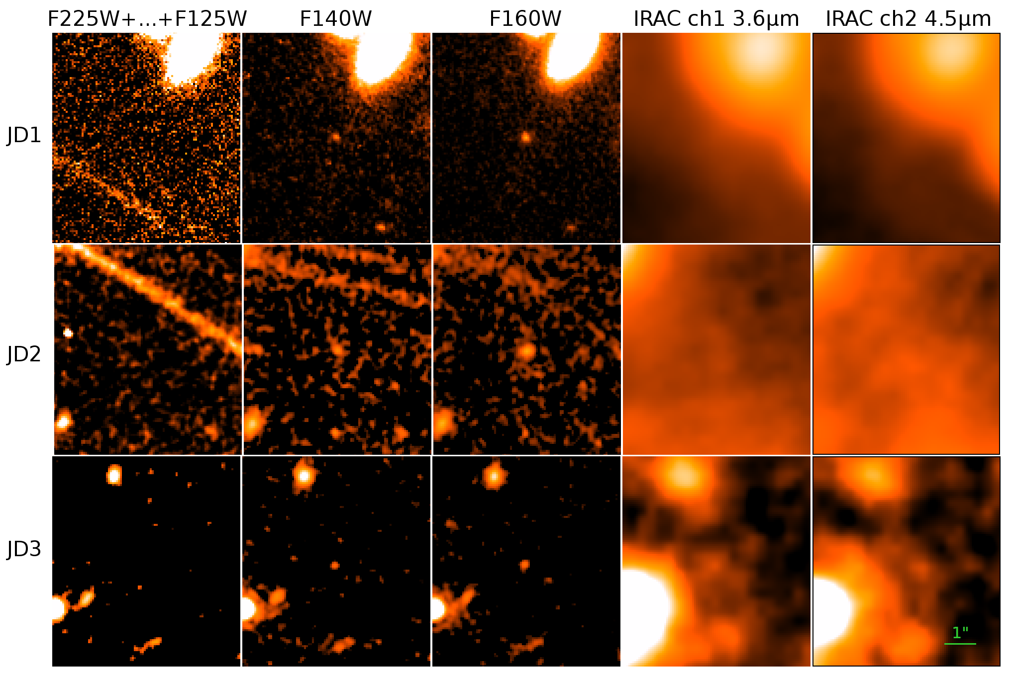
Figure 1.— Image stamps (3.5^′′ $\times$ 3.5^′′) of the three different multiple images of the $z\approx 11$ candidate MACS0647-JD presented in the upper (JD1), middle (JD2), and lower rows (JD3). The five columns show left to right (1) the weighted average of the available HST data from the F225W band to the F125W band (15 bands), (2) the HST WFC3/F140W image, (3) the HST WFC3/F160W image, (4) the Spitzer IRAC 3.6 $\mu$m image, and the Spitzer IRAC 4.5 $\mu$m image. The panels are not displayed in the same brightness scale but are adjusted for better viewability. The very bright nearby stars are not subtracted (as discussed in Section 2.2) in this figure.

2.2. Subtraction of the Bright Stars Around MACS0647

One particularly challenging aspect of doing photometry on the $z\approx 11$ galaxy behind MACS0647 is the presence of an 8th magnitude star only 2 arcminutes away from the cluster core, and 13th, 14th, and 16th magnitude stars in the same $2^{\prime}$ $\times$ $2^{\prime}$ WFC3/IR field.

Clearly, the first step in measuring the Spitzer/IRAC fluxes in the faint $z\approx 11$ multiple images around MACS0647 is the removal of the extended light of nearby Galactic bright stars. Otherwise, our photometric modeling package mophongo will attempt to model the extended stellar light from the bright stars as originating from various bright sources nearby (within a radius of 12”) the $z\approx 11$ multiple images.

Figure 2 shows the four stars that contribute most of the contamination. A high dynamical range, extended PSF model produced by IRSA is combined from observations of stars across a wide range of fluxes. The FITS files can be obtained at this link. We then simply use galfit (Peng et al., 2010) to model and subtract the extended stellar light while masking out the saturated stellar cores as well as all bright objects in the field of view. This process is repeated for exposures lying at a range of roll angles.

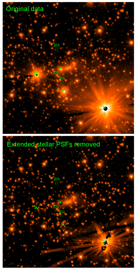
Figure 2.— (upper) The original Spitzer IRAC 3.6$\mu$m image with the four bright stars to be removed, with approximate apparent magnitudes of 8, 13, 14, and 16 (indicated by the green arrows). (lower) The same image as the top panel, but with the extended stellar light subtracted. Bright foreground sources (mostly cluster galaxies) and saturated stellar cores are masked out to allow for an accurate fit to the extended component of stellar light from the bright stars.

2.3. “Column Pull-Down” Artifact

A second artifact that impacts the fidelity of the Spitzer/IRAC imaging observations is the column pull-down artifact, which is relatively large in the case of the MACS0647 cluster data due to the brightness of the foreground stars. These artifacts reduce the intensities in entire columns where the bright objects are located. The Spitzer IRAC basic calibrated data (BCD) pipeline partially corrects for the column pull-downs. However, correcting for this artifact perfectly is extremely challenging, particularly when working with fields with extremely bright sources, such as is the case near the centers of galaxy clusters or where a field has many bright stars such as with MACS0647.

Based on a simple visual inspection of the individual exposures acquired at different roll angles of the telescope, we found that half of the data suffered from column pull-down artifacts oriented such that the first multiple image, JD1, is affected, while for the other half of the data, the second and third multiple images JD2 and JD3 are affected. Figure 3 shows how column pull-down artifact overlaps with the position of JD1 in half of the data while in the other half of the data JD2 and JD3 are impacted. This unfortunate coincidence of various multiple images of MACS0647-JD with “pull-down” artifacts reduces the amount of usable data by a factor of $\approx$2 for each multiple image. We construct one mosaic image for JD1 from exposures with roll angles such that JD1 is not affected by the ”column pull-down” artifact, and similarly we construct a second mosaic image for JD2 and JD3 from exposures with roll angles such these two multiple images are not affected by the ”column pull-down” artifact.

Table 2 Coordinates, estimated magnification factors, and demagnified photometry of the three multiple images of MACS0647-JD: JD1, JD2, and JD3.

	JD1	JD2	JD3	combined
RA (J2000)	06:47:55.731	06:47:53.112	06:47:55.452
Decl. (J2000)	+70:14:35.76	+70:14:22.94	+70:15:38.09
20cmMagnification
(ZITRIN LTM)	6.0${}^{+0.6}_{-0.7}$	5.5${}^{+1.0}_{-0.4}$	2.1${}^{+0.3}_{-0.1}$	13.6${}^{+1.2}_{-0.8}$
F225W	$-22\pm 9$ ($-2.4\sigma$)	$-7\pm 9$ ($-0.8\sigma$)	$6\pm 15$ ($0.4\sigma$)	$-8\pm 7$ ($-1.2\sigma$)
F275W	$-16\pm 9$ ($-1.8\sigma$)	$-6\pm 8$ ($-0.7\sigma$)	$23\pm 12$ ($2.0\sigma$)	$1\pm 5$ ($0.1\sigma$)
F336W	$0\pm 6$ ($0.1\sigma$)	$9\pm 5$ ($1.7\sigma$)	$-12\pm 9$ ($-1.4\sigma$)	$-1\pm 4$ ($-0.2\sigma$)
F390W	$-1\pm 3$ ($-0.4\sigma$)	$0\pm 3$ ($0.1\sigma$)	$0\pm 5$ ($0.1\sigma$)	$-0\pm 2$ ($-0.1\sigma$)
F435W	$0\pm 4$ ($0.0\sigma$)	$8\pm 4$ ($1.7\sigma$)	$2\pm 7$ ($0.4\sigma$)	$3\pm 3$ ($1.1\sigma$)
F475W	$-0\pm 2$ ($-0.1\sigma$)	$-5\pm 3$ ($-1.6\sigma$)	$3\pm 4$ ($0.9\sigma$)	$-1\pm 2$ ($-0.4\sigma$)
F555W	$-0\pm 2$ ($-0.3\sigma$)	$2\pm 1$ ($1.7\sigma$)	$3\pm 2$ ($1.5\sigma$)	$2\pm 1$ ($1.6\sigma$)
F606W	$0\pm 3$ ($0.2\sigma$)	$2\pm 4$ ($0.6\sigma$)	$-0\pm 3$ ($-0.2\sigma$)	$1\pm 2$ ($0.4\sigma$)
F625W	$-6\pm 4$ ($-1.6\sigma$)	$-9\pm 5$ ($-2.1\sigma$)	$11\pm 5$ ($2.3\sigma$)	$-1\pm 3$ ($-0.6\sigma$)
F775W	$1\pm 5$ ($0.1\sigma$)	$-3\pm 9$ ($-0.3\sigma$)	$2\pm 5$ ($0.4\sigma$)	$-0\pm 4$ ($-0.0\sigma$)
F814W	$0\pm 1$ ($0.0\sigma$)	$-0\pm 1$ ($-0.4\sigma$)	$-1\pm 1$ ($-0.7\sigma$)	$-0\pm 1$ ($-0.6\sigma$)
F850LP	$-0\pm 5$ ($-0.1\sigma$)	$0\pm 5$ ($0.0\sigma$)	$3\pm 7$ ($0.4\sigma$)	$1\pm 3$ ($0.2\sigma$)
F105W	$2\pm 2$ ($0.9\sigma$)	$3\pm 2$ ($1.1\sigma$)	$1\pm 2$ ($0.6\sigma$)	$2\pm 1$ ($1.5\sigma$)
F110W	$-1\pm 2$ ($-0.8\sigma$)	$1\pm 2$ ($0.3\sigma$)	$3\pm 2$ ($1.7\sigma$)	$1\pm 1$ ($0.8\sigma$)
F125W	$-0\pm 2$ ($-0.3\sigma$)	$1\pm 3$ ($0.4\sigma$)	$1\pm 2$ ($0.4\sigma$)	$1\pm 1$ ($0.4\sigma$)
F140W	$10\pm 2$ ($5.2\sigma$)	$9\pm 2$ ($4.9\sigma$)	$12\pm 2$ ($5.5\sigma$)	$11\pm 1$ ($9.1\sigma$)
F160W	$27\pm 4$ ($7.4\sigma$)	$25\pm 4$ ($7.0\sigma$)	$20\pm 3$ ($7.4\sigma$)	$24\pm 2$ ($12.4\sigma$)
IRAC [3.6]	62.0$\pm$ 26.5 (2.3$\sigma$)	14.4$\pm$ 23.4 (0.6$\sigma$)	57.5$\pm$ 23.5 (2.4$\sigma$)	44.6$\pm$ 14.1 (3.2$\sigma$)
contamination	166.9 (269%)	13.9 (97%)	27.6 (48%)
IRAC [4.5]	62.6$\pm$ 18.5 (3.4$\sigma$)	15.5$\pm$ 12.2 (1.3$\sigma$)	53.2$\pm$ 33.7 (1.6$\sigma$)	43.8$\pm$ 13.5 (3.2$\sigma$)
contamination	135.8 (217%)	11.5 (74%)	21.8 (41%)

3. Photometry and Size Measurements

3.1. HST

Since the HST observations we make use of in the study of MACS0647-JD are identical to that in Coe et al. (2013), for simplicity and consistency with the Coe et al. (2013) study, we make use of the same photometry presented in that study. In Coe et al. (2013), fluxes are measured in isophotal apertures using SExtractor (Bertin and Arnouts, 1996). The detection image is constructed from a weighted mean of the five WFC3 IR bands. The flux uncertainties are estimated based on the rms noise measured in apertures of similar size from the nearby background. This approach directly accounts for the contribution of correlated noise in mosaic images. Table 2 lists the HST photometry after correction for the lensing magnification (see section 3.4).

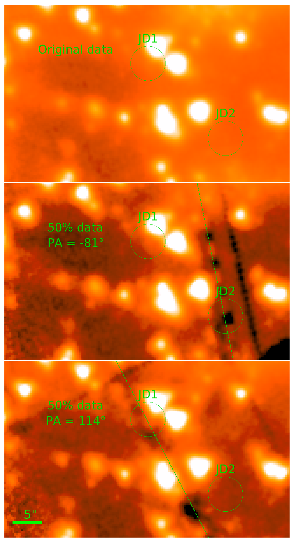
Figure 3.— Illustration of the Spitzer/IRAC observations available over various multiple images of MACS0647-JD showing the impact that “column pull-down” artifacts from bright stars have on the images (even after correction). This artifact is especially apparent after subtraction of the extended stellar light from original data (upper panel). Half of the Spitzer/IRAC exposures are such that the “column pull-down” artifact runs through JD2 (middle panel) and JD3, while the other half of the exposures are such that this same artifact runs through JD1 (lower panel). We therefore only make use of that half of the Spitzer/IRAC observations unaffected by the artifact in measuring fluxes for the individual sources.

3.2. Spitzer/IRAC

The Spitzer/IRAC data we use in deriving fluxes for the various multiple images of MACS0647-JD are based on individual exposures taken with rotation angles such that the “column pull-down” artifact does not overlap the sources on which we are performing photometry.

Because of the high density of sources in the Spitzer/IRAC observations, it is necessary to model and subtract flux from neighboring sources before doing photometry on the faint multiple images of interest. As in previous work by our team (Labbé et al., 2006, 2010, 2013, 2015) and other teams (Shapley et al., 2005; Grazian et al., 2006; Laidler et al., 2007; Merlin et al., 2015), we use the high-resolution HST observations as a template for modeling the lower-resolution Spitzer/IRAC observations. It has been shown by simulations that using a high-resolution prior greatly reduces the fraction of sources contaminated by neighbors in Spitzer/IRAC data. Labbé et al. (2015) estimate the improvement in the fraction of contaminated sources to be as much as 80% to 12%. In deriving a template for each source, we take directly the sextractor-segmented HST F160W image, then convolve each segmented object with a mathematical mapping from the HST PSF to the IRAC PSF.

The IRAC PSF model is derived from a large number ($\approx$600) of warm exposures, with spatial variation across the detector taken into account. We then select stars in the HST F160W image (26 of them in this study), and compute the mathematical mapping to the IRAC PSF for each star. The mapping is parameterized by a number of basis functions and their corresponding coefficients. Using the selected stars as anchors, the coefficients, are interpolated across the entire field of view, which gives us a model of the PSF as a function of spatial position. Finally, the amplitude of each PSF mapped segment is allowed to vary in order to minimize the residual. Figure 4 shows that most of the neighboring sources around the targets are well-modeled and reasonably subtracted from the data. Thanks to both the depth of our new Spitzer/IRAC data and use of a more sophisticated photometry procedure, we are able to improve the quality of the Spitzer/IRAC photometry relative to that of Coe et al. (2013).

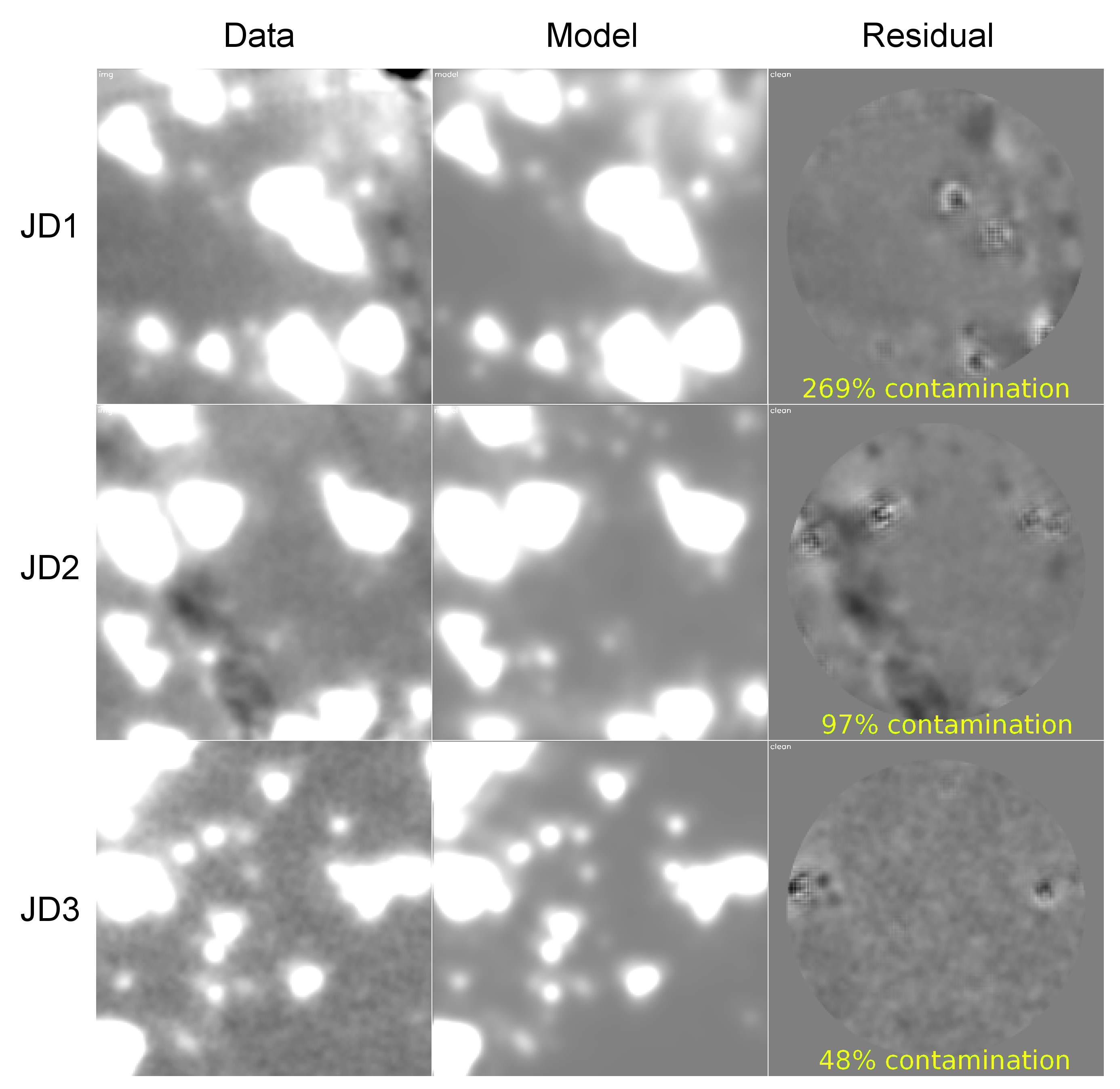
Figure 4.— Illustration of the view we obtain at $3.6\mu$m with Spitzer/IRAC of the various multiple images of MACS0647-JD, i.e., JD1, JD2, and JD3 (shown in the upper, middle, and lower rows), based on our model of the light from the neighboring sources. The left column shows the original Spitzer/IRAC images, the middle column shows our model for the light from neighboring sources, and the right column shows the residual images after subtraction of all neighboring objects. As the quality of the subtractions is similar in both the $3.6\mu$m and $4.5\mu$m, only the $3.6\mu$m image is shown here. The relatively modest flux apparent in the Spitzer/IRAC imaging data, after subtraction of the light from the nearby neighbors, provides strong evidence that MACS0647-JD is unlikely to be a low-z interloper, consistent with the earlier conclusions of Coe et al. (2013) and Pirzkal et al. (2015).

We then measure the fluxes of our targets using circular apertures with radius of 0.9” and then divide this flux by the expected fraction of encircled energy inside this radius for a point source. The fitting errors of neighbouring objects are also taken into account, by adding in quadrature with the Poisson noise measured by the apertures on the source-subtracted image. The Spitzer/IRAC photometry are presented in Table 2.

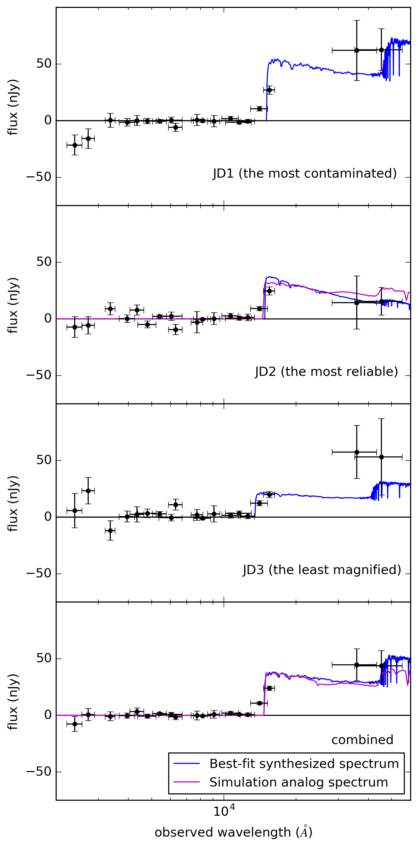
Figure 5.— Best-fit stellar population model fits (blue lines) to the observed photometry (black points) of the three multiple images, MACS0647-JD1, JD2, and JD3 (panels from the top), as a function of the observed wavelength. The lowest panel shows similar fits to the combined photometry for MACS0647-JD. Shown for comparison are spectra from the EAGLE simulations that serve as analogues to EAGLE (magenta lines). These simulated spectra are slightly shifted from z=10 to z=11 and normalized to the best-fit synthesized spectra at rest-frame 1600 Å to better match the observed spectra.

3.3. Spectral Energy Distribution

Figure 5 plots the de-magnified spectral energy distribution (SED) of MACS0647-JD1, JD2, JD3, and their stacked values. Compared to JD1 and JD3, our primary target, JD2, has a tentatively steeper rest-frame UV slope, although still consistent with the measurements of the other two multiple images. Since most of the systematics have been removed, this suggests the Poisson noise still dominate the uncertainty of ultra-faint objects.

Of the three multiple images, JD2 is recognized as perhaps the best target because of its high magnification and its being more separated from bright neighbors. JD1 is the most magnified but is also the most contaminated (by a nearby cluster galaxy), while JD3 is the least contaminated but also the faintest, having the lowest magnification factor from gravitational lensing.

3.4. Lensing Magnification

The magnification factors of JD1, JD2, and JD3 are estimated by a suite of recently-constructed light-traces-mass (LTM) models constructed using the methods of Zitrin et al. (2009) and Zitrin et al. (2014). The models are constrained by multiply lensed images including those of MACS0647-JD. The uncertainties correspond to the 68.3% confidence level from the model MCMC minimization, unless, these are exceeded by the magnifications in an area of 1”x1” around each multiple image, or the variation between different best-fit models probed in the modeling procedure.

The magnification factors used in this work are different from those used by Coe et al. (2013). Those are estimated from a Lenstool model, and are 8.4, 6.6, and 2.8 for JD1, JD2, and JD3, respectively.

3.5. Size Measurements

We use the high spatial resolution HST data to measure physical sizes for the various multiple images of MACS0647-JD. We perform the measurement using galfit (Peng et al., 2010) and use it to fit PSF-convolved Sérsic profiles to the F160W data. The derivation of the F160W PSF we utilize is described in §3.2.

Based on the fits we perform with galfit, we find that JD1 and JD2 are slightly resolved (see also Coe et al., 2013). Their measured effective radii are 0.068$\pm$0.017” and 0.062$\pm$0.017”, respectively, while we find JD3 to be unresolved (i.e., $<$0.063^′′, 1-$\sigma$). We converted the observed image-plane sizes into physical sizes, by demagnifying each source radius by the square root of the model-estimated magnification factor. The results are presented in Table 3. The mean intrinsic half-light radius measured for MACS0647-JD is 105$\pm$28 pc.

Interestingly enough, the size we measure for MACS0647-JD is similar to the observed sizes of local star cluster complexes (e.g., 30 Doradus) and giant molecular clouds, which are on the order of 30-100 pc (Johansson et al., 1998; Murray et al., 2011). The inferred stellar mass and star formation rate of MACS0647-JD (see §4) are much higher, of course, than local giant molecular clouds. The fact that there are such large differences can be mainly attributed to the fact that mass density roughly scales as $(1+z)^{3}$ and thus star formation density was much, much higher in the early universe.

Table 3 Inferred properties of MACS0647-JD based on the measured photometry and light profile fitting for JD1, JD2, JD3, and a weighted average of the photometry for JD1, JD2, and JD3.

object	z	MUV,AB	log10(age/yr)	20cmlog10(mass/
M⊙)	20cmlog10(sfr/
(M⊙/yr))	20cmrest-frame
UV slope
(measured)	20cmrest-frame
UV slope
(best-fit
model)	20cmintrinsic
half-light radius
(pc)
JD1	11.4${}^{+0.4}_{-1.0}$	$-$20.3$\pm$0.3	8.6${}^{+0.1}_{-2.2}$	9.2${}^{+0.2}_{-1.5}$	0.8${}^{+0.9}_{-0.5}$	$-$1.0$\pm$0.8	$-$2.3	110$\pm$40
JD2	11.2${}^{+0.4}_{-1.0}$	$-$19.6$\pm$0.3	6.8${}^{+1.9}_{-1.8}$	7.7${}^{+1.3}_{-0.3}$	0.9${}^{+1.1}_{-0.7}$	$-$2.7$\pm$1.7	$-$2.9	100$\pm$40
JD3	10.1${}^{+0.9}_{-0.4}$	$-$20.4$\pm$0.5	8.7${}^{+0.1}_{-3.7}$	8.8${}^{+0.2}_{-1.5}$	0.3${}^{+1.2}_{-0.2}$	$-$0.7$\pm$0.9	$-$2.3	$<$170
Stack	11.1${}^{+0.5}_{-0.9}$	$-$20.1$\pm$0.2	8.6${}^{+0.1}_{-2.1}$	9.1${}^{+0.2}_{-1.4}$	0.6${}^{+0.7}_{-0.4}$	$-$1.3$\pm$0.6	$-$2.3

4. Stellar population properties

4.1. Stellar Population Modeling

We derive the age, the mass, and the star formation rate, by fitting synthesized stellar population spectra to the measured photometry (Figure 5) using FAST (Kriek et al., 2009). For the stellar population synthesis model, we choose Bruzual & Charlot (2003). This particular model has a wider range in stellar ages (from 0.1 Myr to the age of the Universe) than the other options (Maraston, 2005; Maraston & Strömbäck, 2011; Conroy & Spergel, 2011), which may be advantageous for modelling galaxies at very high redshifts. We adopt a Chabrier initial mass function (Chabrier et al., 2003), which is derived from observations of various parts of the Galaxy while the other two IMFs, Salpeter (1955) and Kroupa (2002), are derived from observations of the solar neighborhood.

For simplicity, we assume a constant star formation history. We adopt the dust law of Kriek & Conroy (2013). It is a flexible attenuation law that varies with the spectral type of galaxies, and is derived from galaxies at redshifts up to 2. This option is more flexible and is derived from galaxies at higher redshifts compared to the other two options, Calzetti et al. (2000) and Cardelli et al. (1989). For metallicity, we choose the lowest possible value (Z = 0.004) given the expected young age of the galaxy at z$\approx$11. Finally, we keep the maximum possible extinction small, A_v = 0.1, as observed to be typical at such high redshifts for galaxies from the latest ALMA observations (Aravena et al., 2016; Bouwens et al., 2016b; Dunlop et al., 2016) of galaxies in the Hubble Ultra Deep Field (Beckwith et al., 2006).

4.2. SED Fitting Results

The physical properties we have inferred for each of the multiple images of MACS0647-JD and the weighted average are compiled in table 3. For its age, the three multiple images-combined constraint is log₁₀(age/yr) = 8.6${}^{+0.1}_{-2.1}$, while with the optimal target - JD2 alone, the estimated age is substantially younger - only log₁₀(age/yr) = 6.8${}^{+1.9}_{-1.8}$, although still consistent within the uncertainty. For its stellar mass, the constraint based on the combined photometry of the three multiple images is log₁₀(M_∗/M_⊙) = 9.1${}^{+0.2}_{-1.4}$, while using only JD2, the stellar mass is log₁₀(M_∗/M_⊙) = 7.7${}^{+1.3}_{-0.3}$. The star formation rate based on the combined photometry is $4^{+16}_{-2}$ M_⊙ yr^-1 while the value based on the JD2 photometry is $7^{+84}_{-6}$ M_⊙ yr^-1.

As only the 4.5$\mu$m Spitzer/IRAC channel reaches the rest-frame optical and there are large uncertainties on the measured flux in that band, the age is not strongly constrained. This means that our stellar mass estimates are strongly correlated with the adopted stellar population age. Specifically, if we consider only low values of the age, i.e., log₁₀(age/yr) $\approx$ 6.8, we infer stellar masses $\approx$1 dex lower than if higher values of the age, i.e., log₁₀(age/yr) $\approx$ 8.6, are considered.

The new constraints we have obtained from SED-fitting are similar to the first-order estimates of Coe et al. (2013), who derived a star formation rate of $\approx$ 4 $M_{\odot}$ yr^-1 and a stellar mass on the order of $10^{8}-10^{9}M_{\odot}$. Figure 6 shows the $\chi^{2}$ fit values for JD1, JD2, JD3 individually and the combined constraint.

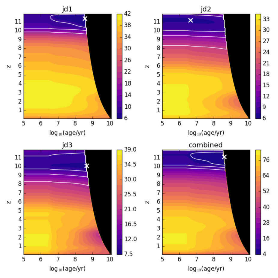
Figure 6.— Our $\chi^{2}$ fit results to MACS0647-JD vs. stellar population age and redshift, assuming a constant star formation rate. Results are shown based on the photometry for JD1, JD2, JD3, as well as the combined photometry. The color bar provides the scale for the $\chi^{2}$ values. The best-fit values of redshift and age are marked by the white crosses’s. The white contours in each panel show the 1$\sigma$, 2$\sigma$, and 3$\sigma$ confidence intervals. The black region on the right side of each plot shows the disallowed region of parameter space, where the stellar population ages exceed the age of the Universe at the corresponding redshifts.

The absolute UV magnitudes, $M_{UV}$, of JD1, JD2, and JD3 are $-$20.49, $-$19.91, and $-$19.32, respectively. Their average value is $-$19.91. We assume the best-fit redshifts from FAST, which are z=11.4, z=11.2, and z=10.1 for JD1, JD2, and JD3, respectively. $M_{UV}$ is measured at a rest-frame wavelength of 1600Å. Since the observed wavelength ($\approx$1.9 $\mu$m) is not covered by any filters, we infer $M_{UV}$’s from FAST’s best-fit spectra.

Using the H${}_{160}-$[3.6] color (Wilkins et al., 2016), we find that the rest-frame UV slope, $\beta$, of the stacked photometry is $-$1.3$\pm$0.6, and is $-$2.7$\pm$1.7 for JD2 alone. Calculating $\beta$ directly from the color of F160W and IRAC [3.6], however, does not take into account of the Lyman break shifting into the F160W filter which occurs at z$\approx$10.5. Another way to estimate $\beta$ is to take the values from the best-fit stellar population models, which are found to be $-$2.3 and $-$2.9 for the stacked photometry and JD2 respectively. These estimates for $\beta$ are mostly bluer than our estimates based on colors themselves, but are highly consistent with the age and dust extinction we estimate for the source.

The use of different stellar population parameters to model the photometry of MACS0647-JD results has only a modest impact on the result. Use of another stellar-population model (e.g. Conroy & Spergel, 2011), dust model (e.g. Calzetti et al., 2000), or metallicities (e.g. solar metallicity: Z = 0.02) only results in $\approx$10 - 20$\%$ changes in the derived properties. If we do allow a larger maximum possible extinction of A_v = 1.0, then the age can decrease by $\approx 70\%$ while the mass increases by $\approx 30\%$, which together can cause the estimated star formation rate to increase by a factor of 3. As expected, use of a Salpeter (1955) IMF significantly increases the stellar mass ($\approx 70\%$) we infer for MACS0647-JD.

The stellar population modeling we have performed here should benefit from significantly improved constraints on the redshift of MACS0647-JD from HST grism data. These data included 12 orbits of HST grism data obtained as part of a cycle 21 program (GO-13317, PI: Coe). Fixing the redshift to z=11.2 and z=11.1 for JD2 and the combined photometry (their best-fit redshift derived by FAST), we arrive at tighter constraints on the derived age. Using the JD2 and combined photometry, we derive an age of log₁₀(age/yr) = 6.8${}^{+1.0}_{-1.8}$ and log₁₀(age/yr) = 8.6 (errors less than 0.1 dex when redshift is fixed to $z=11.1$), respectively.

The Bruzual & Charlot (2003) models used by FAST does not include nebular emission line models. Pacifici et al. (2015) showed that emission lines contamination have a negligible impact on stellar mass estimates for $z\approx 1-3$ star-forming galaxies. However, at $z\approx 10$, the star-formation/ISM conditions of galaxies could be extreme, resulting in a significant contribution to the photometry by strong Lyman-$\alpha$ and other rest-UV ISM emission lines. This would result in the FAST derived galaxy properties being systematically biased. In order to constrain the impact of nebular emission lines on the derived galaxy properties, we use the Flexible Stellar Population Synthesis code (Conroy, Gunn, & White, 2009) within the Prospector framework (Leja et al., 2017) to obtain best-fit galaxy properties via SED fitting. We use an exponentially declining SFH with an e-folding time of 1 Gyr with redshift fixed at $z=11.1$ and vary the stellar mass, stellar metallicity, age, and dust extinction (following Calzetti et al. 2000) between reasonable parameter space with a tophat prior. The median deviation for the age and stellar metallicity estimates between models with and without nebular contribution (emission + continuum) is consistent with no statistically significant difference. However, the tests we run suggest the stellar mass estimates would be systematically overestimated by $\approx 0.7\pm 0.3$ dex when emission lines are not included. Additionally, there is also a slight tendency for the dust extinction to be overestimated when not accounting for the strong nebular lines. We note that our observational data is limited to $\lambda<4.5\mu m$, thus we have no constraints on the rest-frame optical and NIR spectral shape of MACS0647-JD, which is crucial for reliable stellar mass/metallicity estimates.

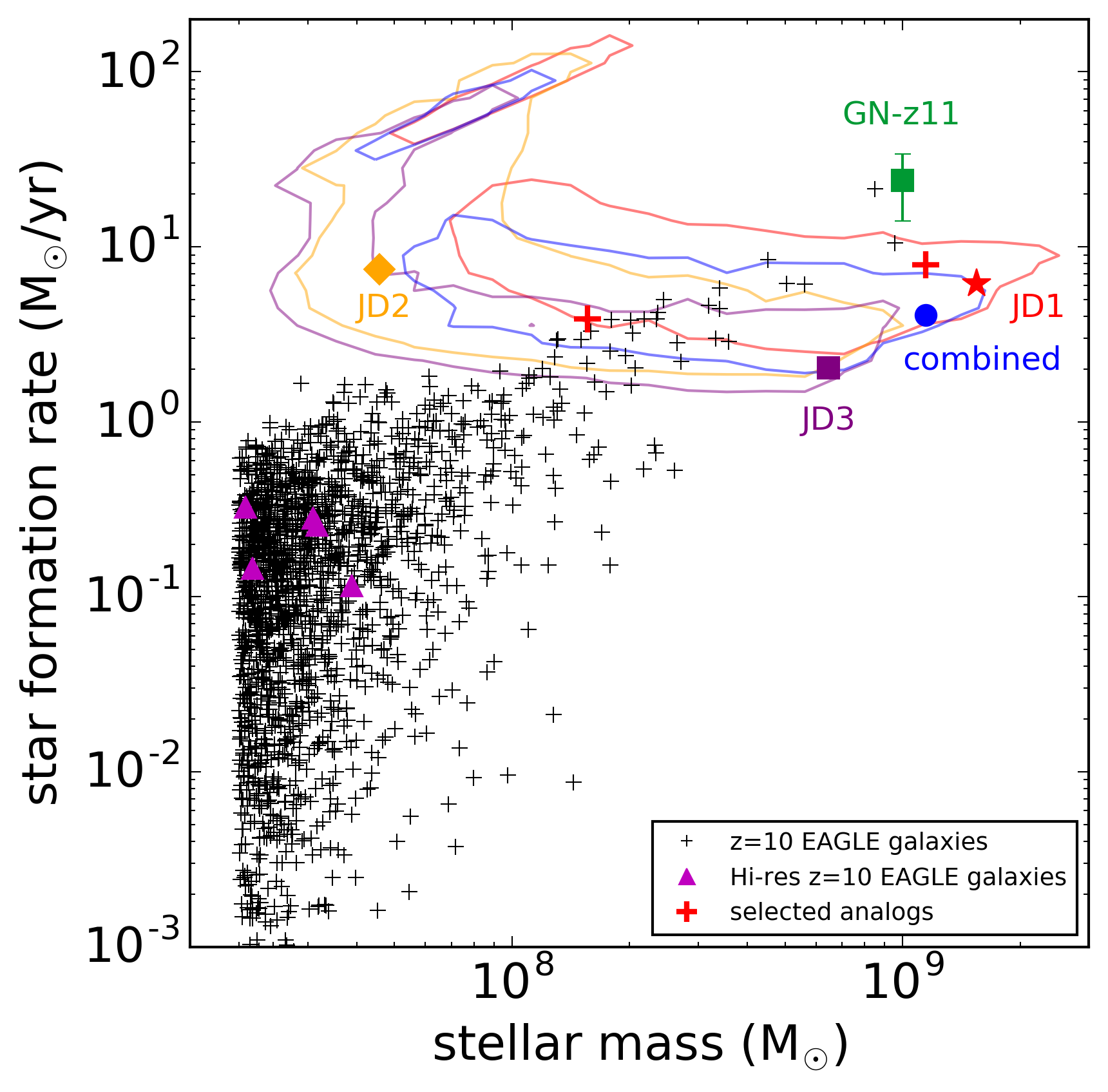
Figure 7.— SFR vs. stellar mass inferred for various multiple images of MACS0647-JD based on stellar-population modeling of the observed photometry. Separate results are plotted for each of the multiple images, i.e., JD1 (red star), JD2 (orange diamond), JD3 (purple square), and a weighted average of the photometry for all three multiple images (blue cross). Their 1-$\sigma$ confidence levels are plotted as solid lines with the same colors. Also plotted for context are the recent $z=11.1$ galaxy GN-z11 reported by (Oesch et al., 2016, green square) and $z\approx 10$ galaxies (black crosses) from EAGLE (corresponding to the closest snapshot in EAGLE to $z\approx 11.1$). Galaxies at the same redshift found in a smaller volume but higher resolution version of the EAGLE simulation are denoted by magenta triangles. The red crosses denote the galaxies from EAGLE whose properties most resemble those of JD2 and the weighted average of each of the multiple images. The inferred properties for MACS0647-JD seem consistent with some of the most massive and the most rapidly star-forming galaxies in the EAGLE simulation.

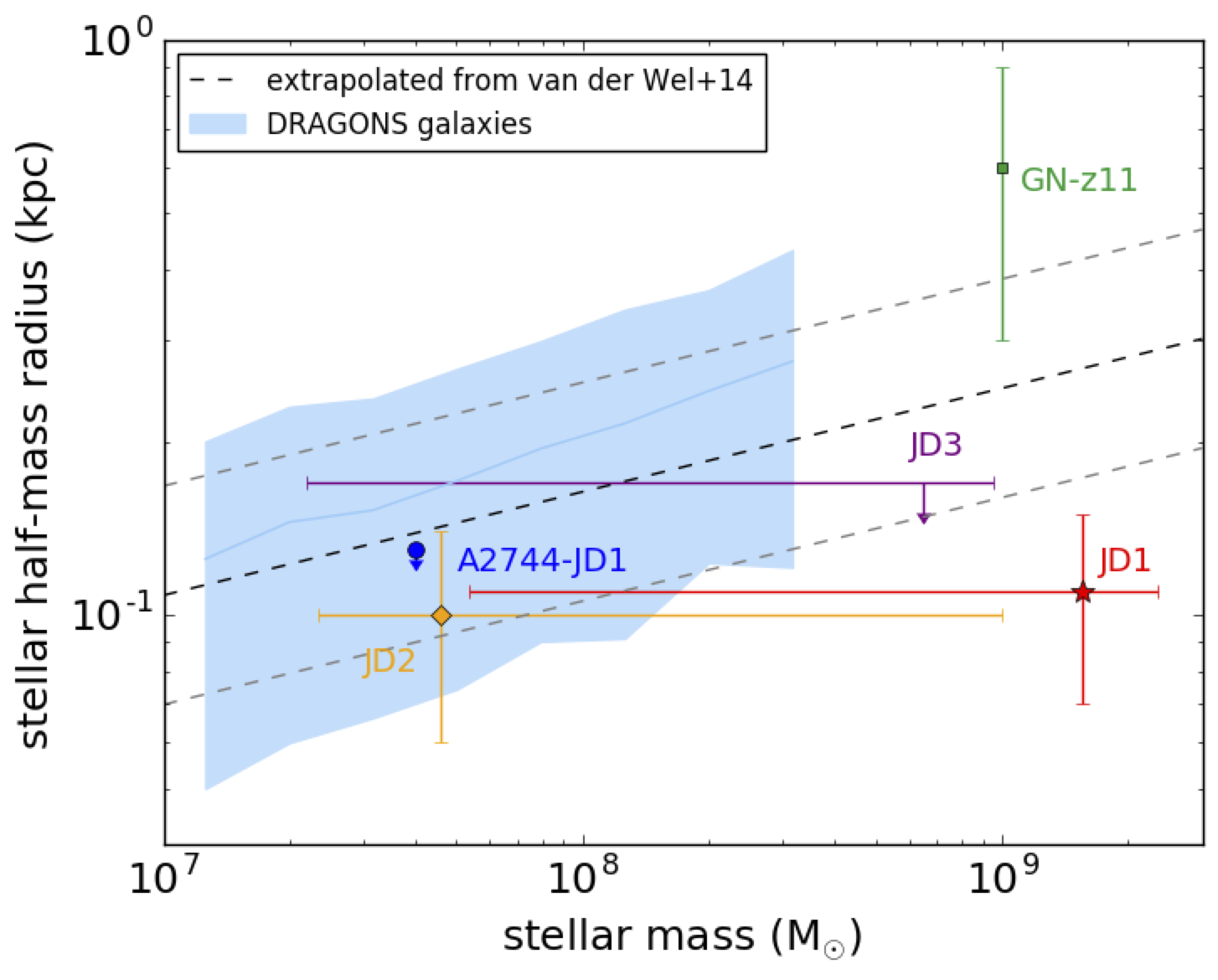
Figure 8.— Stellar mass vs. half-mass radius derived for the different multiple images of MACS0647-JD, the $z=11.1$ galaxy GN-z11 (green square), and the z$\approx$10 galaxy A2744-JD1 (Zitrin et al., 2014, blue circle) compared against similar quantities in the semi-analytical DRAGONS simulation. The light blue line and the shaded area denote the average sizes and the 1-$\sigma$ dispersion of DRAGONS galaxies as a function of stellar mass at z$\approx$10.9. The size-mass relation of DRAGONS galaxies is shown up to $\approx$5$\times$10⁸M_⊙, beyond which the number of galaxies becomes very small. Overplotted as the black dashed line is the size-mass relation of late-type galaxies at $z=2.75$ by van der Wel et al. (2014), extrapolated to $z=11$ using the best-fit scaling with redshift z=2.75 also found in van der Wel et al. (2014) study. The gray dashed lines denote the scatter in the relation extrapolated to $z=11$.

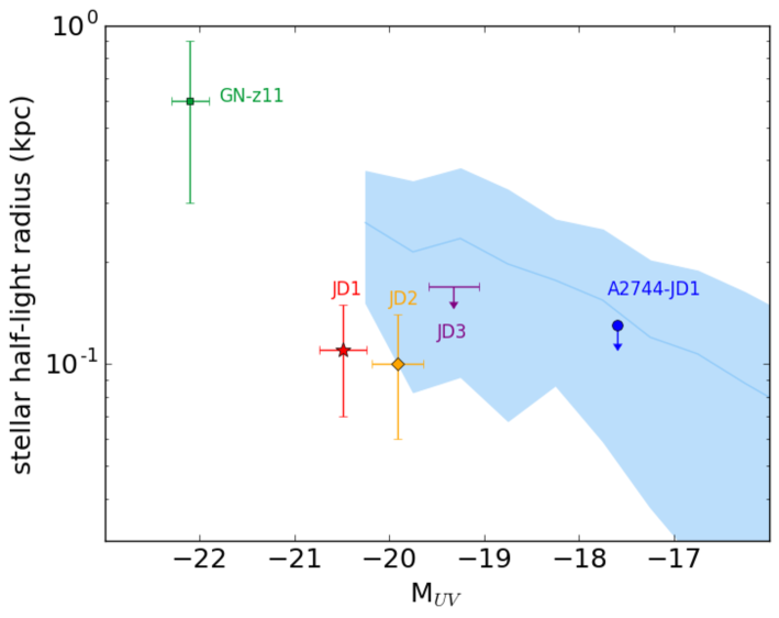
Figure 9.— Half-light radius vs. absolute UV magnitude inferred for each multiple image of MACS0647-JD, GN-z11 (green square), and A2744-JD1 (blue circle). These current observational results for z $\approx$ 10 – 11 galaxies are shown relative to the distribution in parameter space seen in the DRAGONS (Liu et al., 2017) simulations, with the blue shaded region representing the $\pm 1\sigma$ sizes in the simulations and the blue line representing the average size-M_UV relation. The smaller than expected sizes of low luminosity sources at $z\approx 11$ recalls the very small size results at $z\approx 6$-9 (Bouwens et al., 2017b; Kawamata et al., 2015, 2018), where many sources with $\leq$100 pc sizes are found.

5. Comparison with cosmological simulation

It is interesting to compare the present observational results on MACS0647-JD with that found in current state-of-the-art cosmological hydrodynamical simulations. One such simulation is the EAGLE project (Schaye et al., 2015). The simulation successfully captures a diverse range of astrophysical phenomena using various subgrid physics recipes, including radiative cooling, star formation, stellar feedback, AGN feedback, accretion and mergers of supermassive black holes. The amplitude of these effects are tuned to reproduce the observed galaxy stellar mass function, the relation between stellar mass and halo mass, galaxy sizes, and the relation between black hole mass and stellar mass at $z\approx 0$. Encouragingly, the tuned simulation is found to reproduce a number of low-redshift observations not used in setting the subgrid physical prescriptions. These observations include the specific star formation rates and fractions of passive galaxies, the relation between the maximum rotation speed and stellar mass (Tully-Fisher relation), the relations between metallicity (of ISM and stars) and stellar mass, the relation between the luminosity and mass of galaxy clusters, the relation between X-ray luminosity and temperature of the intracluster medium, as well as the column density distributions of intergalactic metals. One might therefore ask whether the physical properties we infer for our $z\approx 11$ candidate are a good match to galaxies in the EAGLE simulation.

We select the analogs from the main run of EAGLE, which simulates a volume of 100³ comoving-Mpc³ with a gravitational resolution of 2.66 kpc (comoving). The EAGLE analogs are selected using the criteria that they have properties (SFR and stellar mass) that are most consistent with that inferred based on the JD2 photometry (the ideal target) as well as on the combined photometry. Figure 7 plots the star formation rate against the stellar mass for MACS0647-JD and EAGLE galaxies taken from the z = 10 snapshot with stellar masses greater than 2$\times$10⁷ M_⊙. The EAGLE simulation is captured in 29 snapshots from z = 20 to z = 0. The snapshot at z = 10 is the most relevant one to this work. We also include galaxies found in a variant of the EAGLE main run that has a smaller volume but higher resolution into the analog selection. The galaxies found in the smaller simulation volume, however, tend to be the less massive and less rapidly star-forming.

Radiative transfer is not implemented within the EAGLE simulation. Rendering images and spectra of EAGLE galaxies requires post-processing of the particle information. In this case we use SKIRT (Camps & Baes, 2015), a radiative transfer with dust processing code that takes snapshots from hydrodynamical simulations as input, to simulate the images and spectra of the EAGLE analogs. Specifically, the position, stellar mass, and age of star particles of the selected analogous galaxies from EAGLE are used as inputs. We compute results using Bruzual & Charlot (2003) stellar population synthesis libraries and the Draine & Li (2007) dust model.

The spatially integrated spectra are overplotted in magenta in Figure 5 on JD2 and the stacked photometry. The spectra are slightly shifted from z=10 to z=11 and normalized to the best-fit synthesized FAST spectra at rest-frame 1600 Å to better compare their shapes. The spectral shapes of the analogs from the EAGLE simulation resemble those seen in the various multiple images of MACS0647-JD.

In terms of stellar population properties, the selected analogs of MACS0647-JD are relatively high mass and with a high SFR relative to the general population found in the EAGLE simulation. This is not surprising given that the observation strategy of CLASH to survey a large number of galaxy cluster lenses at modest depths.

It would not be very meaningful to compare the observed sizes of MACS0647-JD with sources in the EAGLE simulation, since EAGLE lacks the necessary spatial resolution. At z = 11, the gravitational softening length of EAGLE is $\approx$0.2 proper kpc (Schaye et al., 2015), which is greater than the measured sizes of the multiple images JD1 and JD2 (Table 3). We therefore compare our measured sizes with predictions made by another cosmological simulation, DRAGONS (Liu et al., 2017). DRAGONS is a semi-analytical galaxy formation simulation designed to study the galaxy formation and the structure of reionization in the early universe at redshifts between z=35 and z=5 (Mutch et al., 2016). While EAGLE simulates dark matter and gas particles in a fully self-consistent way, the galaxy formation and ionization parts of DRAGONS (Mutch et al., 2016) are semi-analytical models based on a collisionless N-body cosmological simulation called Tiamat (Poole et al., 2016). These physical models are calibrated to a hydrodynamical cosmological simulation called Smaug (Duffy et al., 2014), which simulates a much smaller volume (10 $h^{-1}$ cMpc each side, but includes important physics like the interaction between radiation and gas. The overall less computational-intensive scheme of DRAGONS means it can simulate features that EAGLE lacks, such as the interaction between radiation and baryons. It also means that DRAGONS has a higher spatial resolution. At z=11, the gravitational softening length is $\approx$75 proper pc (Poole et al., 2016), which is slightly smaller than the radius we infer for MACS0647-JD.

In Figure 8 we plot the stellar half-mass radius against the stellar mass for MACS0647-JD and DRAGONS galaxies. We also consider an extrapolation of the size-mass relation derived for $0<z<3$ late-type galaxies from the 3D-HST and CANDELS program (van der Wel et al., 2014). This size-mass relation is extrapolated from z=2.75 to z=11 using the size-mass redshift evolution derived in that study. Specifically, it is

$$R_{\textrm{eff}}/\textrm{kpc}=10^{\textrm{A}}(M_{*}/5\times 10^{10}M_{\odot})^{\alpha}((1+z)/3.75)^{-0.75}\textrm{,}$$ (1)

where A = 0.51$\pm$0.01, $\alpha$ = 0.18$\pm$0.02, and z = 11. Note that the power-law dependence on $(1+z)$ for the size-mass relation is not especially surprising given that $\rho\propto(1+z)^{3}$ and hence $r\propto M^{1/3}(1+z)^{-1}$ (e.g., Ferguson et al., 2004). The observed size of the different multiple images of MACS0647-JD is generally smaller than expected, but the comparison is challenging due to significant uncertainties in our stellar mass estimates.

A more direct evaluation of the observed sizes of MACS0647-JD relative to that seen in the simulations can be achieved by conducting the comparisons at a fixed UV luminosity (Figure 9). It is clear that MACS0647-JD is $\approx$2$\times$ smaller in terms of its size at $M_{UV,AB}\approx-20$ mag than sources in the DRAGONS simulation. The present results bring to mind the unexpectedly small observed sizes found by Bouwens et al. (2017a, b) and Kawamata et al. (2015, 2018) from the Hubble Frontier Fields (Lotz et al., 2017) or the proto-globular cluster candidates from Vanzella et al. (2017). In the former studies (see also Ma et al., 2018), it was suggested that the small sizes likely resulted from just a fraction of a galaxy lighting up with star formation. However, with only one size measurement for a $>$$-$21 mag galaxy at $z\approx 11$, we are clearly very limited in the conclusions we can draw.

6. Summary

We describe the use of new, deep Spitzer/IRAC observations we obtained of a particularly bright $z\approx$11.1 galaxy MACS0647-JD to constrain its physical properties. MACS0647-JD benefits from substantial lensing magnification from the galaxy cluster MACS0647, with the three multiple images with estimated magnification factors of 6.0, 5.5, and 2.1. The source is unique in that it is one of two moderately bright galaxy candidate known at $z\approx$11 – the other being GN-z11 (Oesch et al., 2016) – which are amenable to such detailed study.

The new Spitzer/IRAC observations (50 hours per band: PI Coe) probe much fainter than the previously existing 5-hour observations of this candidate. The deeper observations allow us to place improved constraints on its stellar mass, age, and dust properties. After subtracting the flux from neighboring sources and combining the three different multiple images, we obtain a secure $>$3$\sigma$ detection of the source in the Spitzer/IRAC data.

We then derive constraints on its stellar population properties, including age, stellar mass, star formation rate, and rest-frame UV slope. The age, stellar mass, and rest-frame UV slope we estimate for MACS0647-JD based on a stack of the photometry are log₁₀(age/yr) = 8.6${}^{+0.1}_{-2.1}$, log₁₀(M_∗/M_⊙) = 9.1${}^{+0.2}_{-1.4}$, and $-$1.3$\pm$0.6, respectively. Using the least-contaminated and most magnified image yields lower but still consistent values of log₁₀(age/yr) = 6.8${}^{+1.9}_{-1.8}$, log₁₀(M_∗/M_⊙) = 7.7${}^{+1.3}_{-0.3}$, and $-$2.7$\pm$1.7.

We compared the stellar mass and star formation rate we derive for MACS0647-JD with predictions for the source from the cosmological hydrodynamical simulation, EAGLE, and find that MACS0647-JD resembles the more massive and rapidly star-forming ones in EAGLE.

We also measure the physical half-light radius of MACS0647-JD and find 105$\pm$28 pc. Interestingly enough, the observed size we measure is $\approx 2\times$ smaller than the mean sizes of $\approx-$20 mag sources in the DRAGONS simulations. The very small observed sizes of MACS0647-JD (vs. expectations) is evocative of similarly small sizes of $z\approx$6-10 sources recently reported behind the HFF clusters (Kawamata et al., 2015; Bouwens et al., 2017a, b; Kawamata et al., 2018; Vanzella et al., 2017; Zitrin et al., 2014). Comparisons with observed sizes in EAGLE are not useful, given that the larger spatial extent of the softening length relative to the observed sizes at $z\approx 11$.

It is remarkable that we are able to map out the overall shape of the SED of a galaxy (to $\approx$0.4$\mu$m) at $z\approx 11$ with HST and Spitzer Space telescopes and to constrain its stellar population age, stellar mass, and dust content. Unfortunately, we are limited in terms of the conclusions we could draw from this one source, and so we will be conducting follow-up analyses on a larger sample of lensed sources in the epoch of reionization (z $>$ 6) in datasets such as CLASH (Postman et al., 2012), Hubble Frontier Fields (Lotz et al., 2017), and SURFS UP (Bradač et al., 2014).

References

- Aravena et al. (2016) Aravena, M., Decarli, R., Walter, F., et al. 2016, ApJ, 833, 71
- Beckwith et al. (2006) Beckwith, S. V. W., Stiavelli, M., Koekemoer, A. M., et al., 2006, AJ, 132, 1729
- Bertin and Arnouts (1996) Bertin, E. and Arnouts, S. 1996, A&AS, 117, 39
- Bouwens et al. (2010) Bouwens, R. J., Illingworth, G. D., González, V., et al. 2010, ApJ, 725, 1587
- Bouwens et al. (2011a) Bouwens, R. J., Illingworth, G. D., Oesch, P. A., et al. 2011a, ApJ, 737, 90
- Bouwens et al. (2011b) Bouwens, R. J., Illingworth, G. D., Labbe, I., et al. 2011b, Nature, 469, 504
- Bouwens et al. (2012) Bouwens, R. J., Illingworth, G. D., Oesch, P. A., et al. 2012, ApJ, 752, L5
- Bouwens et al. (2014) Bouwens, R. J., Bradley, L., Zitrin, A., et al. 2014, ApJ, 795, 126
- Bouwens et al. (2015) Bouwens, R. J. et al., 2015, ApJ, 803, 34
- Bouwens et al. (2016a) Bouwens, R. J., Oesch, P. A., Labbé, I., et al. 2016a, ApJ, 830, 67
- Bouwens et al. (2016b) Bouwens, R. J., Aravena, M., Decarli, R., et al. 2016b, ApJ, 833, 72
- Bouwens et al. (2017a) Bouwens, R. J., Illingworth, G. D., Oesch, P. A., et al. 2017a, ApJ, 843, 41
- Bouwens et al. (2017b) Bouwens, R. J., van Dokkum, P. G., Illingworth, G. D., et al. 2017b, arXiv:1711.02090
- Bradač et al. (2014) Bradač, M. et al., 2014, ApJ, 785, 108
- Bradley et al. (2014) Bradley, L. D., Zitrin, A., Coe, D., et al. 2014, ApJ, 792, 76
- Brammer et al. (2014) Brammer, G. B., Pirzkal, N., McCullough, P. et al. 2014, ISR WFC3 2014-03
- Bruzual & Charlot (2003) Bruzual, G., Charlot, S., 2003, MNRAS, 344, 1000
- Calzetti et al. (2000) Calzetti, D. et al., 2000, ApJ, 533, 682
- Camps & Baes (2015) Camps, P., M. Baes, 2015, A&C, 9, 20
- Cardelli et al. (1989) Cardelli, J. A. et al., 1989, ApJ, 345, 245
- Chabrier et al. (2003) Chabrier, G. 2003, ApJ, 586L, 133
- Coe et al. (2013) Coe, D. et al., 2013, ApJ, 762, 32
- Conroy, Gunn, & White (2009) Conroy, C., Gunn, J. E., White, M., 2009, ApJ, 699, 486
- Conroy & Spergel (2011) Conroy, C., Spergel, D. N., 2011, ApJ, 726, 36
- Draine & Li (2007) Draine, B. T., Li, A., 2007, ApJ, 657, 810
- Duffy et al. (2014) Duffy, A. R., Wyithe, J. S. B., Mutch, S. J. et al. 2014, MNRAS, 443, 3435
- Dunlop et al. (2016) Dunlop, J. S., McLure, R. J., Biggs, A. D., et al. 2017, MNRAS, 466, 861
- Ellis et al. (2013) Ellis, R. S., McLure, R. J., Dunlop, J. S., et al. 2013, ApJ, 763, L7
- Ferguson et al. (2004) Ferguson, H. C., Dickinson, M., Giavalisco, M. et al. 2004, ApJ, 600, 107
- Finkelstein et al. (2012) Finkelstein, S. L., Papovich, C., Ryan, R. E., et al. 2012b, ApJ, 758, 93
- Finkelstein et al. (2015) Finkelstein, S. L., Ryan, R. E., Jr., Papovich, C., et al. 2015, ApJ, 810, 71
- Grazian et al. (2006) Grazian, A., Fontana, A., de Santis, C., et al. 2006, A&A, 449, 951
- Hashimoto et al. (2018) Hashimoto, T., Laporte, N., Mawatari, K. et al. 2018, Nature, 557, 392
- Hoag et al. (2018) Hoag, A., Bradač, M., Brammer, G., et al. 2018, ApJ, 854, 39
- Huang et al. (2016) Huang, K.-H. et al., 2016, ApJ, 817, 11
- Ishigaki et al. (2015) Ishigaki, M., Kawamata, R., Ouchi, M., et al. 2015, ApJ, 799, 12
- Ishigaki et al. (2018) Ishigaki, M., Kawamata, R., Ouchi, M. et al., 2018, ApJ, 854, 73
- Johansson et al. (1998) Johansson, L. E. B., Greve, A., Booth, R. S. et al. 1998, A&A, 331, 857
- Kawamata et al. (2015) Kawamata, R., Ishigaki, M., Shimasaku, K., Oguri, M., & Ouchi, M. 2015, ApJ, 804, 103
- Kawamata et al. (2018) Kawamata, R., Ishigaki, M., Shimasaku, K., et al. 2018, ApJ, 855, 4
- Kriek et al. (2009) Kriek, M. et al., 2009, ApJ, 700, 221
- Kriek & Conroy (2013) Kriek, M., Conroy, C., 2013, ApJ, 775L, 16
- Kron (1980) Kron, R. G. 1980, ApJS, 43, 305
- Kroupa (2002) Kroupa, P., 2002, Science, 295, 82
- Labbé et al. (2006) Labbé, I., Bouwens, R., Illingworth, G. D., & Franx, M. 2006, ApJ, 649, L67
- Labbé et al. (2010) Labbé, I., González, V., Bouwens, R. J., et al. 2010a, ApJ, 708, L26
- Labbé et al. (2013) Labbé, I., Oesch, P. A., Bouwens, R. J., et al. 2013, ApJ, 777, L19
- Labbé et al. (2015) Labbé, I. et al., 2015 ApJS, 221, 23
- Laidler et al. (2007) Laidler, V. G., Papovich, C., Grogin, N. A., et al. 2007, PASP, 119, 1325
- Laporte et al. (2016) Laporte, N., Infante, L., Troncoso Iribarren, P., et al. 2016, ApJ, 820, 98
- Leja et al. (2017) Leja, J. and Johnson, B. D. and Conroy, C. and van Dokkum, P. G. and Byler, N. 2017, ApJ, 837, 170L
- Liu et al. (2017) Liu, C., Mutch, S. J., Poole, G. B., et al. 2017, MNRAS, 465, 3134
- Livermore et al. (2017) Livermore, R., Finkelstein, S. L., Lotz, J. M. 2017, ApJ, 835, 113
- Lotz et al. (2017) Lotz, J. M., Koekemoer, A., Coe, D., et al. 2017, ApJ, 837, 97
- Ma et al. (2018) Ma, X., Hopkins, P. F., Boylan-Kolchin, M., et al. 2018, MNRAS, 477, 219
- Maraston (2005) Maraston, C. et al., 2005, MNRAS, 362, 799
- Maraston & Strömbäck (2011) Maraston, C., Strömbäck, G., 2011, MNRAS, 418, 2785
- McLeod et al. (2015) McLeod, D. J., McLure, R. J., Dunlop, J. S., et al. 2015, MNRAS, 450, 3032
- McLeod et al. (2016) McLeod, D. J., McLure, R. J., & Dunlop, J. S. 2016, MNRAS, 459, 3812
- McLure et al. (2013) McLure, R. J., Dunlop, J. S., Bowler, R. A. A., et al. 2013, MNRAS, 432, 2696
- Merlin et al. (2015) Merlin, E., Fontana, A., Ferguson, H. C., et al. 2015, A&A, 582, A15
- Mitra et al. (2015) Mitra, S., Choudhury, T. R., & Ferrara, A. 2015, MNRAS, 454, L76
- Murray et al. (2011) Murray, N. 2011, ApJ, 729, 133
- Mutch et al. (2016) Mutch, S. J., Geil, P. M., Poole, G. B. et al. 2016, MNRAS, 462, 250
- Oesch et al. (2009) Oesch, P. A., Carollo, C. M., Stiavelli, M., et al. 2009, ApJ, 690, 1350
- Oesch et al. (2013) Oesch, P. A., Bouwens, R. J., Illingworth, G. D., et al. 2013, ApJ, 773, 75
- Oesch et al. (2016) Oesch, P. A. et al., 2016, ApJ, 819, 129
- Oke & Gunn (1983) Oke, J. B., & Gunn, J. E. 1983, ApJ, 266, 713
- Ouchi et al. (2010) Ouchi, M., Shimasaku, K., Furusawa, H., et al. 2010, ApJ, 723, 869
- Pacifici et al. (2015) Pacifici, C., da Cunha, E., Charlot, S., et al. 2015, MNRAS, 447, 786
- Peng et al. (2010) Peng, C. Y. et al., 2010, AJ, 139, 2097
- Pirzkal et al. (2015) Pirzkal, N. et al., 2015, ApJ, 804, 11
- Poole et al. (2016) Poole, G. B., Angel, P. W., Mutch, S. J. et al. 2016, MNRAS, 459, 3025
- Postman et al. (2012) Postman, M. et al., ApJS, 199, 25
- Robertson et al. (2013) Robertson, B. E., Furlanetto, S. R., Schneider, E., et al. 2013, ApJ, 768, 71
- Robertson et al. (2015) Robertson, B. E., Ellis, R. S., Furlanetto, S. R., & Dunlop, J. S. 2015, ApJ, 802, 19
- Salpeter (1955) Salpeter, E. E., 1955, ApJ, 121, 161
- Schaye et al. (2015) Schaye, J. et al., 2015, MNRAS, 446, 521
- Schenker et al. (2013) Schenker, M. A., Robertson, B. E., Ellis, R. S., et al. 2013, ApJ, 768, 196
- Schmidt et al. (2014) Schmidt, K. B., Treu, T., Trenti, M., et al. 2014, ApJ, 786, 57
- Shapley et al. (2005) Shapley, A. E., Steidel, C. C., Erb, D. K., et al. 2005, ApJ, 626, 698
- Stanway, Bunker, & McMahon (2003) Stanway, E. R., Bunker, A. J., & McMahon, R. G. 2003, MNRAS, 342, 439
- Stark (2016) Stark, D. P. 2016, ARA&A, 54, 761
- van der Wel et al. (2014) van der Wel, A. et al., 2014, ApJ, 788, 28
- Vanzella et al. (2017) Vanzella, E., Calura, F., Meneghetti, M., et al. 2017a, MNRAS, 467, 4304
- Wilkins et al. (2016) Wilkins, S. M., Bouwens, R. J., Oesch, P. A., et al. 2016, MNRAS, 455, 659
- Yan & Windhorst (2004) Yan, H., & Windhorst, R. A. 2004, ApJ, 612, L93
- Zheng et al. (2012) Zheng, W., Postman, M., Zitrin, A., et al. 2012, Nature, 489, 406
- Zitrin et al. (2009) Zitrin et al., 2009, MNRAS, 396, 1985
- Zitrin et al. (2014) Zitrin, A., Zheng, W., Broadhurst, T. et al., 2014, ApJ, 793, 12