On the Use of Fast Radio Burst Dispersion Measures as Distance Measures

Abstract

Fast radio bursts appear to be cosmological signals whose frequency-time structure provides a dispersion measure. The dispersion measure is a convolution of the cosmic distance element and the electron density, and contains the possibility of using these events as new cosmological distance measures. We explore the challenges of extracting the distance in a robust manner, and give quantitative estimates for the systematics control needed for fast radio bursts to become a competitive distance probe. The methodology can also be applied to assessing their use for mapping electron density fluctuations or helium reionization.

I Introduction

Fast radio bursts (FRB) are microsecond emissions of radio signals, detected with power in the tens of milli-Jansky or greater range lorimer07 ; thronton13 ; spitler14 ; petroff16 ; shannon18 ; chime19 ; ravi19 . Several dozen FRB are known, with eleven giving repeated signals consisting of more than one hundred pulses altogether spitler16 ; askap19 ; chime19 ; chime19b . The repeat nature seems to disfavor cataclysmic origins such as compact object collisions, and instead FRB are generally regarded as radiation emitted from a compact object with a high magnetic field, such as a magnetar katz16 ; katz18 ; kumar17 ; lu18 ; lyutikov17 ; metzger17 ; 1810.05836 .

FRB show a characteristic sweep in frequency with time, interpreted as a dispersion of the signal propagating through plasma, and the degree of sweep and hence dispersion is quantified by the dispersion measure (DM). At these radio frequencies, the DM depends on the path length through the ionized medium and the electron density. Typical DM of FRB can be several hundred to a few thousand in units of parsecs/cm³. This is greater than expected from lines of sight within the Milky Way galaxy, plus three FRB have been localized sufficiently well to identify their host galaxies and measure their distances spitler16 ; tendulkar17 ; bannister19 ; ravi19b , so FRB are regarded as originating at cosmological distances.

FRB are expected to be useful probes of astrophysics. In particular, they could provide a good map of the baryon distribution, magnetic fields and turbulence in the IGM, helium reionization, and might serve as a new tool for measuring cosmological distances to high redshifts $z\gtrsim 1$, e.g.  macquart13 ; zhang14 ; mcquinn14 ; zhou14 ; macquart15 ; walters18 . A new cosmological distance measure would be exciting, and useful, if it could be made sufficiently robust and competitive in precision to existing cosmological distance probes such as Type Ia supernovae standard candles and baryon acoustic oscillations standard rulers. Many of the systematic uncertainties would differ from other distance probes and thus provide an important crosscheck.

We explore the possibility of FRB serving as a robust distance probe. We emphasize that the purpose of the article is not to claim that they can do so, but rather to bring together the FRB and cosmology communities so they appreciate quantitative estimates of the systematics control that would be required, in a fairly general form. In Sec. II we describe the relation of dispersion measure to distance measure, the comparison with other distance probes, and some of the systematics challenges. Section III investigates the influence of the systematics and quantifies how tightly they need to be controlled in order to give competitive cosmological constraints. We summarize and discuss future avenues of research in Sec. IV.

II From Dispersion Measure to Distance Measure

The dispersion measure does not directly give the distance to the FRB but rather an integral of the distance elements weighted by the electron density. That is,

$${\rm DM}=\int_{t_{e}}^{t_{o}}c\,dt\,n_{e}(t)\,(1+z(t))^{-1}\ ,$$ (1)

where $t_{e/o}$ is the time of emission/observations, $dt$ is the time interval or proper distance, $n_{e}$ is the (proper) electron number density, and the final factor of $1/(1+z)$, where $z$ is the redshift, arises from transformations of the frequency and time between the emitter and observer frames. Specifically, the signal at a given frequency $\nu$ is delayed in plasma, with respect to travel time in vacuum, by $dt/\nu^{2}$ (all quantities measured in the local frame), and hence in the observer frame the contribution to the arrival time delay, the DM, scales as $dt/(1+z)$. See for example 0309200 ; 0309364 .

II.1 General properties

There are several aspects of Eq. (1) to note:

• DM is not purely cosmological but receives contributions from the electron density in the burst environment and host and observer galaxies.

• If the density weighting were perfectly known, DM is a distance combination, say $\int dt/a^{2}$, that is not trivially related to the luminosity distance or angular diameter distance, both of which depend on $\int dt/a$, or the time/age interval $\int dt$, where $a=1/(1+z)$ is the cosmic expansion factor.

• DM is not a pure distance measure but a density weighted sum of distance intervals, i.e. a convolution of functions.

While the second item represents a special cosmological opportunity, the first and third pose challenges to the use for cosmological model constraints. We examine them in order.

II.2 Component Contributions

It is useful to start with the first bullet and write the DM in more generality with dependence on observational characteristics. As stated in the bullet and the literature, DM receives several contributions:

$$DM_{\rm obs} = DM_{\rm env}(\hat{n}_{\rm env},t)+DM_{\rm host}(\hat{n}_{\rm host})$$ (2)

$$+DM_{\rm cos}(\hat{n}_{\rm cos},\vec{\theta})+DM_{\rm MW}(\hat{n}_{\rm MW})\ .$$

The first term is the dispersion measure induced in the local vicinity directly by the fast radio burst source, e.g. the plasma associated with the physical mechanism and its immediate environment. This DM contribution may depend on the orientation $\hat{n}_{\rm env}$ of the signal propagation with respect to, say, the source rotation axis. There may also be a time dependence among repeat pulses as the line of sight intersects different magnetic field or plasma regions. Both it and the host galaxy term contain the same $1/(1+z)$ factor from the observer frame transformation as Eq. (1), though we do not explicitly list a redshift dependence above.

The next term comes from the host galaxy and the fourth term comes from our own Milky Way galaxy, each possibly depending on where the FRB is in the sky and within its host galaxy. The third term is what we seek, the cosmological contribution that depends on the cosmic distance of the source, which in turn depends on a set of cosmological model parameters $\vec{\theta}$. In addition, it can have a direction dependence due to the imperfectly homogeneous intergalactic medium.

Let us discuss these individually. DM_MW can vary from about ten to several hundred along a typical line of sight, but we will assume that maps of electron density and DM in our Milky Way galaxy are sufficiently good that given a FRB sky position we can subtract the contribution DM_MW. See, for example, 1610.09448 ; ne2001 . The host galaxy contribution is more problematic. Given an estimate of the host galaxy morphology and mass, one could assign a value to DM_host, but $\hat{n}_{\rm host}$ may not be clear, nor may the degree of variation with line of sight for that galaxy type. For the Milky Way, DM can vary between lines of sight by over two orders of magnitude 1610.09448 ; ne2001 , with the Galactic center magnetar, SGR J1745-2900, having a measured of DM=1778 eatough13 . One might hope that this scatter could average to an unbiased mean over many FRB host galaxies, but this is not guaranteed, especially if there are observational selection effects preferring certain lines of sight (e.g. perpendicular to a disk plane or see macquart15b ). Presumably this is less of an issue for radio signals than in the optical, unless FRBs are preferentially located in the galactic center regions or embedded in molecular clouds or supernovae remnants. We will keep open the possibility of a potential bias in the mean.

For the local environment contribution DM_env we have similar issues with directionality. Again, we will allow the possibility that a mean over many FRB at the same redshift may not give an unbiased DM estimate to that redshift. We do not include time variation as written in Eq. (2); see Appendix A for further discussion.

Finally, let us address spatial variations directly in the cosmological contribution to DM. Due to inhomogeneities in the intergalactic medium (IGM) and halos along the line of sight, i.e. fluctuations in electron density, different lines of sight to the same redshift will have different DM. Simulations 1309.4451 ; 1812.11936 indicate the standard deviation in DM_cos may be 200, i.e. 20%, at $z=1$ (also see 1712.01280 ; prochaska19 ). A reasonable approximation out to $z\approx 3$ is $\sigma_{\rm DM}\approx 210\sqrt{z}$. If one approximates DM$\approx 1000\,z$ then

$$\frac{\sigma_{\rm DM,cos}}{\rm DM_{cos}}\approx\frac{20\%}{\sqrt{z}}\ .$$ (3)

II.3 Cosmological Sensitivities

The second bullet of Sec. II.1 notes the unique nature of FRB DM with respect to the distance element dependence. If all other issues could be controlled, DM could potentially offer complementarity with standard distance probes. Let us explore this aspect in further detail.

If the DM_cos contribution could be reliably estimated, and if the electron density follows the homogeneous universe dependence of $n_{e}(z)\sim(1+z)^{3}$, then the integral in DM_cos has the form $\int dt/a^{2}=\int dz\,(1+z)/H(z)$, where $H(z)$ is the Hubble parameter. This differs from the standard luminosity or angular diameter distance form of $\int dt/a=\int dz/H(z)$ and so offers different sensitivities to the cosmological parameters for observations at various redshifts. In particular, one might expect greater sensitivity at higher redshift than in the standard distance case, as well as possible complementarity with standard distance probes.

We compute the Fisher sensitivities $\partial{\rm Observable}/\partial{\rm parameter}$ for the observable being either the FRB DM or the standard distances measured by, e.g., supernovae or baryon acoustic oscillations, and the cosmological parameters being $\Omega_{m}$, the matter density as a fraction of the critical density, and the dark energy equation of state parameters $w_{0}$ (its value today) and $w_{a}$ (a measure of its time variation). The result are shown in Fig. 1.

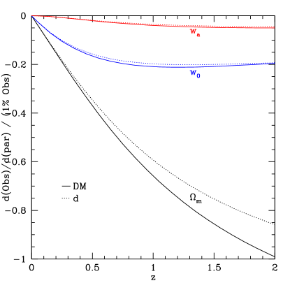
Figure 1: The sensitivity of FRB DM and standard probe distance $d$ to the cosmological model parameters are plotted for 1% measurements of the observables at redshift $z$. Very little difference in sensitivity is seen, indicating not much complementarity between the different types of observations is expected at the cosmological level (although the different systematics entering the probes could make the combination useful).

The extra $1+z$ factor in the integrand for DM makes little difference (of course the sensitivity denominator, here at 1% of the observable goes up as well), in part because the dark energy parameters have the most impact at low redshifts, during cosmic acceleration. For the matter density, there is more of an effect, where indeed the sensitivity is somewhat increased (at the 10% level at $z=1$, 15% level at $z=2$). Since the shapes of the curves remain similar, we do not expect significant complementarity.

To quantify this, we calculate the Fisher information matrix for 15 measurements of 1% precision from $z=0$–1.5 of DM, of standard distance $d$ (it does not matter if it is luminosity or angular diameter distance), and of the combination. In particular, the last, in addition to two separate data sets, could involve simultaneous measurements of the FRB DM and a coincident gravitational wave signal (and hence standard siren distance), if the physical mechanism giving rise to the FRB also produced detectable gravitational wave signals. Also see 1401.0059 ; margalit19 for FRB and gamma ray bursts. Figure 2 illustrates the comparison between the different cases.

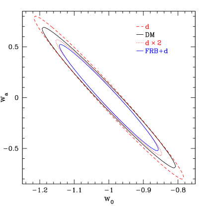
Figure 2: 68% joint confidence contours on the dark energy parameters $w_{0}$ and $w_{a}$ from measurements of standard distances $d$, or FRB DM, or of both (FRB+$d$) to the same redshifts. We also plot the constraints from twice as many standard distance measurements ($d\times 2$), to give the same number of data points as the FRB+$d$ case. All instances include a Planck CMB distance prior.

We see that the DM form, if it can be cleanly deconvolved to attain DM_cos and if it can achieve the same accuracy as standard distance measurements, indeed has a slight advantage over conventional distance probes. It determines $\Omega_{m}$, $w_{0}$, $w_{a}$ to 9%, 11%, 14% better, and the dark energy figure of merit (area of the confidence region) is 24% improved. We also notice that the orientation of the confidence contour is slightly rotated with respect to the standard distance case, indicated some complementarity. If we add together the information from FRB DM and standard distances, there is some slight improvement over simply using standard distances with the same number of measurements, or equivalently total measurement precision. The figure of merit for the FRB+$d$ case is 12% greater than for the $d\times 2$ case.

Of course the big question is whether FRB DM can be used as a precision distance probe without incurring systematics that bias the results. We examine this in the next section.

III Systematics and Required Control

If we misestimate the Milky Way, host galaxy, or FRB environment contributions to the DM then we will offset the cosmological contribution which we may want to use as a distance measure to derive cosmological constraints. Similarly, if we model the electron density function incorrectly this also adds a systematic uncertainty to the distance.

We can use the Fisher information bias formalism (see, e.g., knox98 ; linbias ) to compute the effect of small systematic offsets propagating to biases on cosmological model parameters. In particular, we will focus on the matter density and dark energy parameters, $\Omega_{m}$, $w_{0}$, $w_{a}$, usually constrained by distance probes. The bias on parameter $p_{i}$ is given by

$$\delta p_{i}=\left(F^{-1}\right)_{ij}\sum_{k}\frac{\partial{\mathcal{O}_{k}}}{\partial p_{j}}\frac{1}{\sigma_{k}^{2}}\Delta{\mathcal{O}_{k}}\ ,$$ (4)

where $\Delta{\mathcal{O}_{k}}$ is the difference between the true observable and the one with systematics, $F$ is the Fisher information matrix (and so $F^{-1}$ is the covariance matrix), $\sigma_{k}$ is the statistical uncertainty on the observation, and the index $k$ sums over observations, e.g. redshift shells.

Once the bias $\delta p_{i}$ is determined, one can then impose some requirement on its magnitude as a function of the statistical error on that parameter $\sigma(p)$. For example, limiting $\delta p<0.5\sigma(p)$ is one approach. This, however, does not take into account correlations between parameters, such that a modest bias in multiple parameters in the wrong direction can shift the cosmology well outside the true joint confidence contour, e.g. perpendicular to the major axis of the contours in Fig. 2. Therefore we also consider the change in likelihood due to the bias, using shapiro ; shapiro2

$$\Delta\chi^{2}={\bm{\delta p\,F}}^{(r)}\,{\bm{\delta p}}^{T}\ ,$$ (5)

where $F^{(r)}$ is the Fisher information matrix in the reduced parameter space of interest (marginalized over others) and ${\bm{\delta p}}$ is the vector of parameter biases. Here the space of interest is three dimensional, over $\Omega_{m}$, $w_{0}$, $w_{a}$.

For the observational offsets in the DM cosmology contribution we write

$${\rm DM_{cos}}=b_{a}(z)+b_{m}\int\frac{dz\,(1+z)}{H(z)/H_{0}}\,(1+z)^{n}\ .$$ (6)

Here $b_{a}$ is an additive shift from misestimating other components of DM, e.g. DM_env. It can be redshift dependent because of observational uncertainties that might depend on, e.g., fluence signal to noise, or detector response with frequency as the source redshift gives rise to different observer frame frequencies. We model this simply as $b_{a}(z)=B(1+z)^{m}$. The fiducial value is $B=0$, i.e. no misestimation.

The quantity $b_{m}$ is a constant multiplicative shift, e.g. from misestimated amplitude of baryon density $\Omega_{b}h^{2}$, metallicity, or ionization state, with all redshift dependence absorbed into the $(1+z)^{n}$ factor. Note that $b_{m}$ also has the inverse Hubble constant $1/H_{0}$ absorbed. Its fiducial value is $b_{m}=1$. We take a simple smooth factor $(1+z)^{n}$ factor to represent all redshift dependence other than that already accounted for in $n_{e}(z)\sim(1+z)^{3}$, i.e. deviations from that, including average patchiness $\delta n_{e}/n_{e}$, and metallicity etc. trends. The fiducial value is $n=0$. When all systematic shifts take their fiducial values, then there is no misestimation and no cosmology bias.

We are now set to study how tightly the systematic shifts must be constrained in order not to produce a significant cosmological bias from the data. Beginning with the additive shift, we find that a redshift independent shift ($m=0$) has no effect on the cosmology parameters since it is purely an amplitude offset. (Note that it would affect such parameters as the physical baryon density $\Omega_{b}h^{2}$ or the Hubble constant $H_{0}$, which we do not focus on.) This is equivalent to the situation with a change in the Hubble constant for supernova distances: that only affects the supernova $\mathcal{M}$ amplitude parameter, not the cosmology parameters.

Next we allow the amplitude shift to vary with redshift, i.e. $m\neq 0$. Specifically $b_{a}(z)=B_{\rm mid}[(1+z)/(1+z_{\rm mid})]^{m}$ so $B_{\rm mid}$ is the amplitude at the pivot $z_{\rm mid}$ where this is taken to be the midpoint of the redshift range of observations, i.e. $z_{\rm mid}=0.75$ for FRB covering $z=0$–1.5. The cosmology bias on each parameter will scale linearly with the pivot amplitude, but have a more complicated dependence on the power law index $m$. This is because each cosmology parameter feeds differently into the distance interval at various redshifts; this is also evident in the Fisher sensitivities plotted in Fig. 1. While $\Omega_{m}$ enters strongly already at low redshifts, and $w_{0}$ reaches near maximum impact near the midpoint redshift, the observable is only sensitive to $w_{a}$ at high redshift. Thus we expect little bias in $w_{a}$ for $m<0$ (which weights low redshifts) and more for $m>0$ (weighting high redshifts).

Figure 3 plots the results for an additive systematic of 5% of the DM value at the midpoint redshift; recall the results will scale linearly with amplitude. The biases on the cosmology parameters indeed follow the above physical expectations. We see that for a 5% systematic, the bias in $\Omega_{m}$ can reach $4\sigma$, and near $1\sigma$ on $w_{a}$. Furthermore, the best fit cosmology is biased by up to $\Delta\chi^{2}\approx 20$ for $|m|$ up to one. For a Gaussian joint confidence contour in three parameters, $\Delta\chi^{2}\approx 20$ corresponds to nearly $4\sigma$.

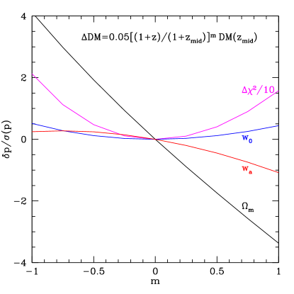
Figure 3: The effect of an additive bias $b_{a}(z)$, due to misestimation of the noncosmological contributions to DM, on the cosmological parameters is plotted vs its redshift power law index $m$. A redshift independent additive bias only affects the DM amplitude, not the main cosmology parameters. Note that $\Delta\chi^{2}$ is plotted divided by 10.

Thus, if we want to restrict the cosmology bias to less than $0.5\sigma$, say, we need to be able to control the additive systematic to $\sim 0.6\%$ if $m=1$. Since the bias on $\Omega_{m}$ dominates, and this appears from Fig. 3 to be fairly linear in $m$, we can phrase the requirement as

$$B_{\rm mid}<0.006\,\frac{1}{m}\,\left(\frac{\rm bias}{0.5\sigma}\right)\,{\rm DM}(z_{\rm mid})\ .$$ (7)

Since DM${}_{\rm cos}(z=0.75)\approx 750$, this requirement implies the systematic uncertainties in other contributions to DM (that vary with redshift) should be smaller than 5 pc/cm³ – a challenging bound. Conversely, if we can control the additive systematic to 5% ($\Delta DM=38$), then we need to ensure that the redshift dependence is quite mild, with power law index $m<0.15$.

For the multiplicative systematic, the scaling of the cosmological parameter biases depends both on the amplitude of the DM offset and the redshift dependence. That is,

$$\Delta{\rm DM_{cos}}=b_{m}\int\frac{dz\,(1+z)}{H(z)/H_{0}}\,\left(\frac{1+z}{1+z_{\rm mid}}\right)^{n}-\int\frac{dz\,(1+z)}{H(z)/H_{0}}\ .$$ (8)

Only for $n=0$ do the biases scale linearly with $(b_{m}-1)$. Note that when $n=0$, the integral value is still redshift dependent and so a constant multiplicative offset does propagate into cosmology. For $n=0$ the redshift dependence of the electron density is as in the usual case, but the amplitude $b_{m}$ can differ due to, e.g., misestimation of the total ionization fraction.

Figure 4 plots the results for a multiplicative systematic of $\pm 2\%$ (i.e. $b_{m}=1\pm 0.02$) of the DM value at the midpoint redshift. Since the biases do not scale linearly with this offset amplitude (except at $n=0$), the curves are not antisymmetric about zero bias. Increasing the systematic further roughly shifts the curves up and down, while preserving their shape.

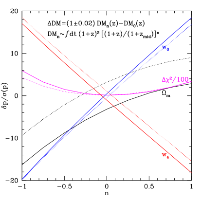
Figure 4: The effect of a multiplicative bias, due to misestimation of the, e.g., electron density contributions to DM, on the cosmological parameters is plotted vs its redshift power law index $n$. Solid curves are for $+2\%$ systematic and dotted curves are for $-2\%$; the biases are not antisymmetric about zero bias except for $n=0$. Note that $\Delta\chi^{2}$ is here plotted divided by 100.

Since for the multiplicative case the systematic DM offset is calculated from the difference between the integral with the added $(1+z)^{n}$ redshift scaling and the standard case with $n=0$, $b_{m}=1$ then even a parameter like $w_{a}$ more sensitive at high redshift shows comparable effects whether $n=+1$ or $n=-1$. In fact, the biases involve a complicated combination of the covariances from all the parameters in the inverse Fisher matrix $F^{-1}$.

For the $n=0$ case, the $\Delta\chi^{2}$ offset in the joint cosmological parameter confidence contours is about 14, which corresponds to $3\sigma$ in three dimensions. This increases for larger $|n|$, reaching $\Delta\chi^{2}=600$ for $n=-1$ for a 2% misestimation. Thus, severe requirements must be placed on systematic uncertainties of both $b_{m}$ and $n$ in order to ensure robust cosmological conclusions.

At $n=0$, the analog of Eq. (7) for the multiplicative systematic is

$$|b_{m}-1|<0.003\,\,\left(\frac{\rm bias}{0.5\sigma}\right)\ .$$ (9)

For $b_{m}=1$, the constraint on the redshift power law index is

$$|n|<0.027\,\,\left(\frac{\rm bias}{0.5\sigma}\right)\ .$$ (10)

In this regime $w_{0}$ and $w_{a}$ are the parameters most sensitive to bias. A value of $n=0.027$ corresponds to a 1% deviation from the standard homogeneous behavior of $(1+z)^{3}$ in the electron density at $z=1.5$ and a $-1.5\%$ deviation at $z=0$.

Note that the requirements on systematics control would tighten further if we combine systematic uncertainties, e.g. allowing both $b_{m}\neq 1$ and $n\neq 0$, or allowing both additive and multiplicative systematics.

IV Discussion and Conclusions

Fast radio bursts are an intriguing astrophysical phenomena that provides a new backlight on the intergalactic medium, and potentially a new distance measure. We investigated the relation between the observed dispersion measure and the cosmological distances, pointing out three main elements: 1) we must understand the noncosmological contributions to DM, and their possible variations with direction, redshift, and time, 2) FRB provide a unique distance measure that is not trivially related to standard luminosity or angular distances, and 3) the convolution of electron density and cosmic distance needs to be considered (see Appendix B for some possibilities).

The main focus was on the first point. We quantified the effects of systematic uncertainties in extraction of $DM_{\rm cos}$ from the observed DM on the cosmological parameters, and found that they could be quite substantial. The amplitude of additive systematics (noncosmological contributions to DM) should be under 0.6% and multiplicative systematics (e.g. electron density variation) smaller than 0.3% in order that the bias in the cosmological parameters is less than $0.5\sigma$ (scaling formulas were provided). Moreover, the redshift dependence of these effects, i.e. power law indices, should be estimated to better than $\delta m<0.15$ and $\delta n<0.027$. These are going be very challenging measurements, even averaging over many FRB, since there could be selection effects.

For example, the DM for the Milky Way varies over $\sim 20$–2000 for different lines of sights through the Galaxy. It is entirely possible that the host contribution to DM could vary similarly, and that might introduce a bias with host galaxy orientation. If there is a systematic bias that is not reduced by $\sqrt{N}$, this would make it very hard to subtract the host galaxy contributions to DM and obtain a robust estimate of DM_cos.

Clearly, for FRB dispersion measures to be used as distance measures, and useful probes of cosmology, systematics will need careful attention and control. There are some hopeful signs.

Upcoming FRB surveys such as shannon18 ; chime19 will provide good localizations so that the redshifts for a fraction of these bursts would be determined from host galaxy identification. These FRBs could better provide the DM contribution from the local environment of bursts and their host galaxies, hopefully reducing the systematics in DM_cos.

Another source of information on distances is contained in pulse broadening. Microsecond scale fluctuations in FRB lightcurves (LCs) are smoothed out due to radio waves scattering off of electron density fluctuations in the IGM and the interstellar medium (ISM) of the host galaxy and the Milky Way. The broadening of pulses in the FRB LC due to scatterings increases with distance to the source, and this effect is more pronounced at lower frequencies; the scattering width scales as $\sim\nu^{-4.4}$. Thus, measurements of the smallest time variation of the FRB LCs can provide information to help improve the determination of DM_cos. The contributions to the FRB pulse broadening by the FRB host galaxy ISM and the Milky Way ISM are suppressed by the geometrical factor $4f(1-f)$ in comparison to the IGM scattering, where $f$ is the ratio of the distances between the FRB source and the host galaxy ISM (treated as a turbulent screen) and the source and us. Therefore, the contribution of the IGM to the FRB pulse width broadening can be important in spite of its much lower electron density compared with the ISM of the host galaxy.

If the IGM turbulence is similar to the Galactic ISM (other than, of course, the large difference in the electron densities), then the pulse broadening in time due to IGM density fluctuations can be obtained by rescaling the ISM contribution by three orders of magnitude to account for the lower electron density in the IGM lorimer13 ; caleb16 ,

$$w_{\rm IGM}=(4\times 10^{-11}\,{\rm ms})\,(1+2\times 10^{-3}DM_{\rm IGM}^{2})\frac{DM_{\rm IGM}^{2.2}}{\nu_{0,{\rm GHz}}^{4.4}}\ .$$ (11)

An alternate possibility is to use the theoretical expression for temporal smearing by IGM turbulence, e.g. macquart13 , instead of rescaling the Galactic ISM scattering observations, to estimate FRB pulse broadening,

$$w_{\rm IGM}(z)=\frac{k_{\rm IGM}D_{\rm eff}}{\nu_{0,GHz}^{4}(1+z_{L})}\int^{z}_{0}\frac{dz^{\prime}\,(1+z^{\prime})^{3}}{H(z^{\prime})/H_{0}}\ ,$$ (12)

where $D_{\rm eff}=D_{L}D_{LS}/D_{S}$, with $D_{L}$, $D_{S}$, $D_{LS}$ the angular diameter distance to the lens, to the source, and between the lens and source, and $k_{\rm IGM}=1.18\times 10^{13}\ {\rm ms\ MHz^{4}}$ is a normalization factor bhattacharya19 .

Eventually, when we have direct redshift measurements for a large sample of FRBs and their pulse widths due to IGM scatterings, then an empirical relation may be obtained for the IGM turbulence properties and scattering broadening. The empirical IGM turbulence property together with the DM measurement would provide a better distance estimate that could be subject to less systematic uncertainty.

Finally, if the goal is astrophysics, then for a given cosmology, FRBs are likely to be excellent probes of electron density fluctuations, and thus the baryon density spectrum on large scales. They may also map the epoch of helium reionization 1902.06981 , or constrain the CMB optical depth degeneracy 1901.02418 ; all these are exciting science topics.

Appendix A Local Environment

Let us briefly consider further the issue of directionality, or variation, of the local environment contribution DM_env. One possibility is that then a mean over many FRB at the same redshift may not give an unbiased DM estimate. There is an element of environmental directionality that could be more problematic. A given direction local to the FRB engine could potentially have a DM varying over time, due to rotation, magnetic field motion, plasma velocity, etc. This is especially relevant for repeating FRBs; recall that accurate redshifts are most likely to be obtained for repeat systems.

Consider the 93 pulses for a repeat outburst of FRB 121102 detected over five hours as described in 1809.03043 . Figure 5 plots the total DM of FRB 121102 vs arrival time, using the data from Table 2 of 1809.03043 . An important distinction is that these are DM_S/N, which may not be the physical DM, and indeed 1804.04101 ; 1811.10748 advocate use of a DM_struc, which relies on an assumption that substructures within a pulse are all emitted at the same time. This may indeed be correct, and in the main text we assume it is and that there is no time variation, but it is worthwhile considering this a little further here. We note that rotation measures can show substantial time variation 1801.03965 , and 1804.04101 state they cannot rule out large variations in DM between pulses. Furthermore, 1804.04101 gives reasons why DM${}_{\rm S/N}>$DM_struc, and yet we see in Fig. 5 significant deviations in DM below as well as above the mean.

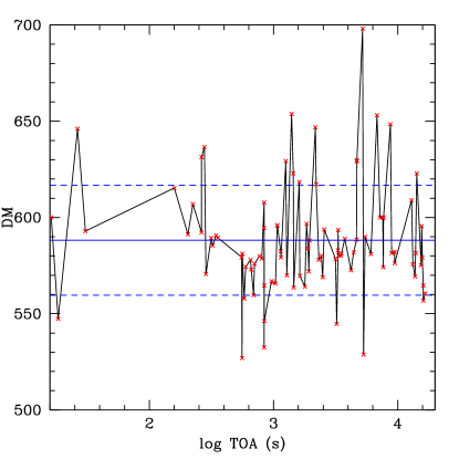
Figure 5: The 93 pulses of the repeating FRB 121102 detected at various times of arrival on August 26, 2017 have variation in total DM (red x’s). While the mean DM=588.2 pc/cm³ (horizontal solid blue line), there is not only a standard deviation 28.6 pc/cm³ (horizontal dashed blue lines) but significant outliers. This may make it unclear what value of DM_env to subtract off to obtain the cosmological DM, but see the text regarding the DM plotted.

The following argument suggests this may not be a physical variation. If the DM were to vary on a time scale of, say, 5 hours, then that suggests that the region responsible for this variation is of size no larger than $10^{14}\,$cm (if the medium is moving at much less than the speed of light then the size is correspondingly smaller than $10^{14}\,$cm). The density of such a medium, in order for it to contribute $\delta{\rm DM}\sim 100$, should be $n_{e}>10^{6}\,{\rm cm}^{-3}$. However, such a medium would block the FRB radiation because of induced-Compton scatterings lu18 ; blandford75 ; wilson82 ; lyubarsky16 . Also see 1707.02923 . Hence the possibility of a large DM variation on a timescale of a few hours (or days) seems difficult to obtain (though there may be a regime of plasma lensing where this can be realized, cf. cordes17 ).

Therefore, while we remain cautious about the possibility of not yet fully identified systematics – merely noting that if one used the maximum deviation from the mean seen for one pulse in Fig. 5 to derive DM_cos this would give a 50% distance error, and if one took the standard deviation value (dashed lines in Fig. 5) this would give a 14% distance error – we will not consider further physical time variations in DM_env.

Appendix B Deconvolution

As an interesting aside, we now turn to the third bullet of Sec. II.1. Suppose that we can successfully separate out the cosmological contribution DM_cos. This involves a convolution of the distance element with the electron density along the signal propagation path. If one assumes a functional form for $n_{e}(z)$, e.g. $n_{e,0}(1+z)^{3}$ as in a perfectly homogeneous, and homogeneously ionized, universe then this is not an issue. Conversely, for an arbitrary function of redshift it is not possible to separate out the cosmological distance; one sees that for

$$n_{e,2}(z)=n_{e,1}(z)\,\frac{dt_{1}(z)}{dt_{2}(z)}\ ,$$ (13)

one could mimic, and misinterpret, cosmology model 1 distances as those of cosmology model 2, for all redshifts.

Observables involving products of the distance with other quantities is not unusual. For example, for strong lensing time delays $\Delta t$ the cosmological distance $D_{\Delta t}$ is entwined with the Fermat factor $\Delta\phi$ of the lensing gravitational potential,

$$\Delta t=D_{\Delta t}\,\Delta\phi\ .$$ (14)

This is merely a multiplicative relation, though, not a convolution in the integrand, and even so is a major systematic for strong lensing, with detailed modeling of the lens matter distribution required for accurate extraction of the cosmic distance.

Closer to the present case is the relation of the observable gamma ray flux of annihilating dark matter particles in a galaxy to the dark matter properties such as mass and cross section. We can write this illustratively as

$$F_{\gamma} \sim \int dr_{\rm los}\int d^{3}v_{1}\int d^{3}v_{2}P(|\vec{v}_{2}-\vec{v}_{1}|)f(\vec{r},\vec{v}_{1})f(\vec{r},\vec{v}_{2})$$ (15)

$$\sim P_{0}\,J[\rho(r)]\ .$$ (16)

Here $f$ is the phase space distribution function of the dark matter particles, $P$ represents particle physics properties, and the $J$ factor involves an integral over the dark matter density (squared). (One can write a similar expression for direct detection of dark matter by nuclear recoil, where the analogous astrophysical factor depends linearly on the dark matter density.) For an arbitrary $J$ factor, i.e. dark matter density profile $\rho(r)$, we cannot determine all the dark matter properties uniquely. Instead one must assume particular models, i.e. functional forms, for the density profile. For FRB, this corresponds to a model for $n_{e}(z)$. Any error in the model could lead to a systematic error in the cosmic distances, and vice versa.

In fact, in the dark matter case 1707.07019 there are clever mathematical methods for treating a fairly general convolution function. These are based on convex hulls and give a piecewise continuous solution, but require the function to be monotonic. (Another application of convex hulls to eigenvector bounds for an arbitrary dark energy equation of state is discussed in 0908.2637 .) While in a homogeneous universe the function $n_{e}(z)$ is indeed monotonic, in this case we already know the functional form and do not need to use the theorem. We do not particularly expect $n_{e}(z)$ to be monotonic, as we know the realistic intergalactic medium is patchy, as discussed in Sec. II.2 and 1309.4451 ; 1812.11936 . Furthermore, $n_{e}$ contributions to DM_cos also arise (roughly equal to the IGM contribution 1309.4451 ; 1812.11936 ) from the line of sight intersecting galaxy halos, and this is emphatically nonmonotonic.

Thus the convex hull approach does not seem apt, unless we seek bounds on the cosmic contribution. Note that a model independent principal component approach to cosmic reionization, e.g. 0705.1132 , could be adapted to the late time ionization fraction and combined with the convex hull eigenvector bound approach of 0908.2637 – if we were interested in bounds on cosmic distances rather than the distances themselves.

References

- (1) D.R. Lorimer, M. Bailes, M.A. McLaughlin, D.J. Narkevic, F. Crawford, A Bright Millisecond Radio Burst of Extragalactic Origin, Science 318, 777 (2007)
- (2) D. Thornton et al., A Population of Fast Radio Bursts at Cosmological Distances, Science 341, 53 (2013)
- (3) L.G. Spitler et al., Fast Radio Burst Discovered in the Arecibo Pulsar ALFA Survey, ApJ 790, 101 (2014)
- (4) E. Petroff, E.D. Barr, A. Jameson, E.F. Keane, M. Bailes, M. Kramer, V. Morello,D. Tabbara, W. van Straten, FRBCAT: The Fast Radio Burst Catalogue, PASA 33, e045 (2016)
- (5) R.M. Shannon et al., The dispersion-brightness relation for fast radio bursts from a wide-field survey, Nature 562, 386 (2018)
- (6) M. Amiri et al., Observations of fast radio bursts at frequencies down to 400 megahertz, Nature 566, 230 (2019)
- (7) V. Ravi, The observed properties of fast radio bursts, Monthly Notices of Royal Astronomical Society 482, 1966 (2019)
- (8) L.G. Spitler et al., A repeating fast radio burst, Nature 531, 202 (2016)
- (9) P. Kumar et al., Faint repetitions from a bright Fast Radio Burst source, arXiv:1908.10026 (2019)
- (10) B.C. Andersen et al., CHIME/FRB Detection of Eight New Repeating Fast Radio Burst Sources, arXiv:1908.03507 (2019)
- (11) J.I. Katz, Fast radio bursts — A brief review: Some questions, fewer answers, Modern Physics Letters A, 31, 1630013 (2016)
- (12) J.I. Katz, Fast Radio Bursts, Progress in Particle and Nuclear Physics 103, 1, (2018)
- (13) P. Kumar, W. Lu & M. Bhattacharya, Fast radio burst source properties and curvature radiation model, MNRAS 468, 2726 (2017)
- (14) W. Lu and P. Kumar, On the radiation mechanism of repeating fast radio bursts, MNRAS 477, 2470 (2018)
- (15) M. Lyutikov, Fast Radio Bursts’ Emission Mechanism: Implication from Localization, ApJL 838, L13 (2017)
- (16) B.D. Metzger, E. Berger, B. Margalit, Millisecond Magnetar Birth Connects FRB 121102 to Superluminous Supernovae and Long-duration Gamma-Ray Bursts, ApJ 841, 14 (2017)
- (17) E. Platts, A. Weltman, A. Walters, S.P. Tendulka, J.E.B. Gordin, S. Kandhai, A Living Theory Catalogue for Fast Radio Bursts, arXiv:1810.05836
- (18) S.P. Tendulkar et al., The Host Galaxy and Redshift of the Repeating Fast Radio Burst FRB 121102, ApJ 834, L7 (2017)
- (19) K.W. Bannister, A single fast radio burst localized to a massive galaxy at cosmological distance, Science 365, 565 (2019)
- (20) V. Ravi, A fast radio burst localized to a massive galaxy, Nature 572, 352 (2019)
- (21) W. Deng and B. Zhang, Cosmological implications of fast radio burst/GRB association, ApJL 783, L35 (2014)
- (22) M. McQuinn, Locating the missing baryons with extragalactic dispersion measure estimates, ApJL 780, L33 (2014)
- (23) B. Zhou, X. Li, T. Wang, Y-Z Fan, and D-M Wei, Fast radio bursts as a cosmic probe?, PhRvD 89, 7303 (2014)
- (24) J-P. Macquart et al., Fast Transients at Cosmological Distances with the SKA, Proceedings of Advancing Astrophysics with the Square Kilometre Array
- (25) A. Walters, A. Weltman, B. M. Gaensler, Y-Z Ma, and A. Witzemann, Future Cosmological Constraints From Fast Radio Bursts, ApJ 856, 65 (2018)
- (26) J-P. Macquart, J.Y. Koay, Temporal Smearing of Transient Radio Sources by the Intergalactic Medium, ApJ 776, 125 (2013)
- (27) K. Ioka, Cosmic Dispersion Measure from Gamma-Ray Burst Afterglows: Probing the Reionization History and the Burst Environment, ApJL 598, L79 (2003) [arXiv:astro-ph/0309200]
- (28) S. Inoue, Probing the Cosmic Reionization History and Local Environment of Gamma-Ray Bursts through Radio Dispersion, MNRAS 348, 999 (2004) [arXiv:astro-ph/0309364]
- (29) J.M. Yao, R.N. Manchester, N. Wang, A New Electron Density Model for Estimation of Pulsar and FRB Distances, ApJ 835, 29 (2017) [arXiv:1610.09448]
- (30) J.M. Cordes, T.J.W. Lazio, arXiv:astro-ph/0207156
- (31) R.P. Eatough et al., A strong magnetic field around the supermassive black hole at the centre of the Galaxy, Nature 501, 391 (2013)
- (32) J-P. Macquart, S. Johnston, On the paucity of fast radio bursts at low Galactic latitudes, MNRAS 451, 3278 (2015) [arXiv:1505.05893]
- (33) M. Jaroszynski, Fast Radio Bursts and cosmological tests, MNRAS 484, 1637 (2019) [arXiv:1812.11936]
- (34) M. McQuinn, Locating the “missing” baryons with extragalactic dispersion measure estimates, ApJ 780, L33 (2014) [arXiv:1309.4451]
- (35) J.M. Shull, C.W. Danforth, The Dispersion of Fast Radio Bursts from a Structured Intergalactic Medium at Redshifts , ApJL 852, L11 (2018) [arXiv:1712.01280]
- (36) J.X. Prochaska and Y. Zheng, Probing Galactic haloes with fast radio bursts, MNRAS 485, 648 (2019) [arXiv:1901.11051]
- (37) W. Deng, B. Zhang, Cosmological implications of Fast Radio Burst / Gamma-Ray Burst Associations, ApJL 783, L35 (2014) [arXiv:1401.0059]
- (38) B. Margalit, E. Berger, and B.D. Metzger, Fast Radio Bursts from Magnetars Born in Binary Neutron Star Mergers and Accretion Induced Collapse, arXiv:1907.00016 (2019)
- (39) L. Knox, R. Scoccimarro, S. Dodelson, Impact of Inhomogeneous Reionization on Cosmic Microwave Background Anisotropy, Phys. Rev. Lett. 81, 2004 (1998) [arXiv:astro-ph/9805012]
- (40) E.V. Linder, Biased cosmology: Pivots, parameters, and figures of merit, Astropart. Phys. 26, 102 (2006) [arXiv:0604280]
- (41) C. Shapiro, Biased Dark Energy Constraints from Neglecting Reduced Shear in Weak Lensing Surveys, ApJ 696, 775 (2009) [arXiv:0812.0769]
- (42) S. Dodelson, C. Shapiro, M. White, Reduced Shear Power Spectrum, Phys. Rev. D 73, 023009 (2006) [arXiv:astro-ph/0508296]
- (43) D.R. Lorimer, A. Karastergiou, M.A. McLaughlin, & S. Johnston, On the detectability of extragalactic fast radio transients, MNRAS 436, L5 (2013)
- (44) M. Caleb, C. Flynn, M. Bailes, E.D. Barr, R.W. Hunstead, E.F. Keane, V. Ravi, W. van Straten, Are the distributions of fast radio burst properties consistent with a cosmological population?, MNRAS 458, 708 (2016)
- (45) M. Bhattacharya, P. Kumar and D. Lorimer, Population modelling of FRBs from intrinsic properties, arXiv:1902.10225
- (46) M. Caleb, C. Flynn, B.W. Stappers, Constraining the era of helium reionization using fast radio bursts, MNRAS 485, 2281 (2019) [arXiv:1902.06981]
- (47) M.S. Madhavacheril, N. Battaglia, K.M. Smith, J.L. Sievers, Cosmology with kSZ: breaking the optical depth degeneracy with Fast Radio Bursts, arXiv:1901.02418
- (48) Y.G. Zhang, V. Gajjar, G. Foster, A. Siemion, J. Cordes, C. Law, Y. Wang, Fast Radio Burst 121102 Pulse Detection and Periodicity: A Machine Learning Approach, ApJ 866, 149 (2018) [arXiv:1809.03043]
- (49) V. Gajjar et al, Highest-frequency detection of FRB 121102 at 4-8 GHz using the Breakthrough Listen Digital Backend at the Green Bank Telescope, ApJ 863, 2 (2018) [arXiv:1804.04101]
- (50) J.W.T. Hessels et al, FRB 121102 Bursts Show Complex Time-Frequency Structure, arXiv:1811.10748
- (51) D. Michilli et al, An extreme magneto-ionic environment associated with the fast radio burst source FRB 121102, Nature 553, 182 (2018) [arXiv:1801.03965]
- (52) R.D. Blandford and E.T. Scharlemann, On Induced Compton Scattering by Relativistic Particles, Ap & SS 36, 303 (1975)
- (53) D.B. Wilson, Induced Compton Scattering in Radiative Transfer, MNRAS 200, 881 (1982)
- (54) Y. Lyubarsky and S. Ostrovska, Induced Scattering Limits on Fast Radio Bursts from Stellar Coronae, ApJ 818, 74 (2016)
- (55) Y-P. Yang, B. Zhang, Dispersion Measure Variation of Repeating Fast Radio Burst Sources, ApJ 847, 22 (2017) [arXiv:1707.02923]
- (56) J.M. Cordes,I. Wasserman,J.W.T. Hessels, T.J.W. Lazio, S. Chatterjee, R.S. Wharton, Lensing of Fast Radio Bursts by Plasma Structures in Host Galaxies, ApJ 842, 35 (2017)
- (57) G.B. Gelmini, J-H. Huh, S.J. Witte, Unified Halo-Independent Formalism From Convex Hulls for Direct Dark Matter Searches, JCAP 1712, 039 (2017) [arXiv:1707.07019]
- (58) J. Samsing, E.V. Linder, Generating and Analyzing Constrained Dark Energy Equations of State and Systematics Functions, Phys. Rev. D 81, 043533 (2010) [arXiv:0908.2637]
- (59) M.J. Mortonson, W. Hu, Model-independent constraints on reionization from large-scale CMB polarization, ApJ 672, 737 (2008) [arXiv:0705.1132]