Water Distribution System Design Using Multi-Objective
Particle Swarm Optimisation

Abstract

Application of the multi-objective particle swarm optimisation (MOPSO) algorithm to design of water distribution systems is described. An earlier MOPSO algorithm is augmented with (a) local search, (b) a modified strategy for assigning the leader, and (c) a modified mutation scheme. For one of the benchmark problems described in the literature, the effect of each of the above features on the algorithm performance is demonstrated. The augmented MOPSO algorithm (called MOPSO+) is applied to five benchmark problems, and in each case, it finds non-dominated solutions not reported earlier. In addition, for the purpose of comparing Pareto fronts (sets of non-dominated solutions) obtained by different algorithms, a new criterion is suggested, and its usefulness is pointed out with an example. Finally, some suggestions regarding future research directions are made.

1 Introduction

Design of water distribution systems (WDS) involves various types of challenging optimisation problems which have been investigated in several research papers to date [1]-[13]. An important subset of these problems is the two-objective optimisation problem in which pipe diameters are to be determined with the objectives of minimising the total cost and maximising the network resilience. Recently, Wang et al. [7] have reported a systematic collection of twelve benchmark WDS design problems of various complexities to serve as an excellent starting point for researchers to try out new multi-objective optimisation algorithms and compare their performance with the results available in the literature. Furthermore, they have made the corresponding EPANET [14] source code and the best-known Pareto front data available in the public domain [15].

Table 1: Summary of some of the benchmark WDS design problems presented in [7].

Network	$N_{\mathrm{pipes}}$	$N_{\mathrm{dia}}$	Search	$N_{FE}^{\mathrm{net}}$	$N_{PF}$
			space size
TLN (SP)	8	14	$1.48\times 10^{9}$	15 M	128
NYT (MP)	21	16	$1.93\times 10^{25}$	90 M	627
BLA (MP)	23	14	$2.30\times 10^{26}$	90 M	901
HAN (MP)	34	6	$2.87\times 10^{26}$	90 M	575
GOY (MP)	30	8	$1.24\times 10^{27}$	90 M	480
PES (IP)	99	13	$1.91\times 10^{110}$	150 M	782

Of the twelve benchmark problems presented in [7], six are summarised in Table 1. For a “small problem” (SP), the size of the search space is relatively small, e.g., for the TLN problem, it is $14^{8}\,$=$\,1.48\times 10^{9}$, and it is possible to compute the cost and resilience for each of the $14^{8}$ possible networks to obtain the true Pareto front. In larger problems, including medium and intermediate problems (marked as MP and IP, respectively, in the table), it is not possible to compute the objective function values for each possible network configuration, and a multi-objective evolutionary algorithm (MOEA) is employed to obtain the approximate Pareto front (i.e., set of non-dominated solutions). In these cases, the true Pareto front is not known, but following [7], we will often use the term “Pareto front” (PF) to refer to the set of non-dominated (ND) solutions obtained by the concerned algorithm.

Five MOEAs were used in [7] for each of the benchmark problems. The ND solutions obtained by the five algorithms were combined, and dominated solutions were removed to form the “best-known” PF. The number of solutions ($N_{PF}$) in the best-known PF thus obtained is listed in Table 1 for each benchmark problem. The percentage of solutions contributed to $N_{PF}$ for each problem by each of the five algorithms is given in Table 2. It can be observed that, except for TLN and HAN networks, no single algorithm was able to obtain all of the solutions in the best-known PF.

Table 2: Percentage of solutions contributed by five MOEAs to the best-known Pareto front [7].

Network	% contribution
	NSGA-II	$\epsilon$-MOEA	$\epsilon$-NSGA-II	AMALGAM	Borg
TLN (SP)	100.0	83.1	83.1	98.7	84.4
NYT (MP)	93.8	17.9	24.8	91.7	20.7
BLA (MP)	77.0	30.3	26.3	90.1	28.3
HAN (MP)	100.0	20.5	23.1	89.7	25.6
GOY (MP)	43.3	3.0	58.2	85.1	22.4
PES (IP)	38.1	27.0	10.7	18.6	23.3

The computation effort involved in obtaining the best-known PF can be described in terms of the total number of function evaluations $N_{FE}^{\mathrm{net}}$ by all five algorithms together since no single algorithm was found adequate in general. For the problems in the MP category, $N_{FE}$ was restricted to 600,000 for each of the five algorithms [7], and 30 independent (randomly initiated) runs were performed for each benchmark problem. The total $N_{FE}$ is therefore $N_{FE}^{\mathrm{net}}\,$=$\,600,000\times 30\times 5\,$=$\,90$ million (90 M), as shown in Table 1.

The purpose of this paper is to present a modified multi-objective particle swarm optimisation algorithm (MOPSO+) for WDS design. In particular, we present results for some of the benchmark problems described in [7] and show that the proposed algorithm gives better solutions than the best-known PFs of [7]. The paper is organised as follows. In Sec. 2, we present a new scheme for comparing PFs produced by two algorithms, to be used in subsequent sections to gauge the performance of the MOPSO+ algorithm. In Sec. 3, we describe the local search scheme implemented in MOPSO+. In Sec. 4, we describe the overall MOPSO+ algorithm and point out specifically the changes with respect to the original MOPSO algorithm presented in [16]. We compare the results obtained using MOPSO+ with the best-known PFs for medium problems in Sec. 5. We then point out in Sec. 6 limitations of the local search scheme for larger problems, propose a suitable modification, and show its effectiveness for one of the benchmark problems in the IP category [7]. Finally, we present conclusion of this work in Sec. 7 and comment on related future work.

2 Comparison of Pareto fronts

In comparing the performance of an MOEA with another with respect to a given benchmark problem, we are mainly interested in (a) computation time, (b) the “quality” of the set of ND solutions. Computation time depends on several factors such as the hardware used, programming environment (compiled or interpreted), and whether parallelisation was employed. Because these factors would vary, a more objective metric, viz., the total number of function evaluations $N_{FE}^{\mathrm{net}}$ is used in [7] and also in this work.

To judge the quality of the ND set obtained by an algorithm, the following metrics are commonly used [16],[17] when the decision variables are continuous: (a) generational distance, a measure of how far the obtained ND solutions are from the true Pareto front, (b) spacing, a measure of the spread of solutions throughout the ND set, (c) error ratio, the percentage of the ND solutions which do not belong to the true Pareto-optimal set.

In the context of the benchmark WDS problems considered here, the true Pareto front is not known. In any case, the above metrics are of limited value for the WDS problem because of the discrete nature of the decision variables. From a practical perspective, apart from cost and resilience, the decision maker (DM) may need to take into account other considerations for implementation [4], and it is important to make a large number of options available to the DM. A more meaningful metric is therefore the number of solutions in the best-known PF which the concerned algorithm can contribute [7]. Based on this idea, we propose some new metrics for comparing the PFs obtained by two MOEAs for a given benchmark problem.

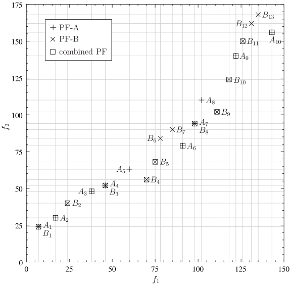
Figure 1: Example showing two sets of ND solutions (Pareto fronts) A and B.

Consider a two-objective problem in which the objective functions $f_{1}$ and $f_{2}$ are to be maximised and minimised, respectively. Fig. 1 shows an example with two sets of ND solutions referred to as PF-A and PF-B. The combined set of ND solutions (marked as “combined PF” in the figure) is obtained by combining solutions from PF-A and PF-B and then removing solutions dominated by any other solutions. The combined PF contains 14 solutions. PF-A, which contains a total of 10 solutions ($A_{1}$ to $A_{10}$), contributes 5 unique solutions ($A_{2}$, $A_{3}$, $A_{6}$, $A_{9}$, $A_{10}$), i.e., solutions which are not present in PF-B. Similarly, PF-B, which contains a total of 13 solutions ($B_{1}$ to $B_{13}$), contributes 6 unique solutions ($B_{2}$, $B_{4}$, $B_{5}$, $B_{9}$, $B_{10}$ $B_{11}$) to the combined PF. The number of common solutions in the combined PF, i.e., solutions which are contributed by PF-A as well as PF-B, is 3 ($A_{1}$/$B_{1}$, $A_{4}$/$B_{3}$, $A_{7}$/$B_{8}$). Note that some of the solutions have been rejected from the original PFs, viz., 2 solutions ($A_{5}$, $A_{8}$) from PF-A and 4 solutions ($B_{6}$, $B_{7}$, $B_{12}$ $B_{13}$) from PF-B.

We use the following nomenclature to describe the above scenario: $N_{A}^{t}\,$=$\,10$, $N_{A}^{u}\,$=$\,5$, $N_{A}^{c}\,$=$\,3$, $N_{A}^{r}\,$=$\,2$ for PF-A, and $N_{B}^{t}\,$=$\,13$, $N_{B}^{u}\,$=$\,6$, $N_{B}^{c}\,$=$\,3$, $N_{B}^{r}\,$=$\,4$ for PF-B. The superscripts t, u, c, r stand for total, unique, common, and rejected, respectively. Note that $N_{A}^{c}$ and $N_{B}^{c}$ must be equal by definition, and we will denote them by $N^{c}$. Clearly, for this example, we cannot say that PF-A is better than PF-B (or vice versa) since each of them has contributed some unique solutions to the combined set.

Consider now the case $N_{A}^{u}\,$=$\,0$, $N_{B}^{u}\,$=$\,4$. In this case, PF-B is certainly better than PF-A because it contributes some unique solutions while PF-A contributes none. In other words, we can do without the information provided by PF-A since PF-B provides all of the solutions which PF-A would have contributed to the combined front ($N^{c}$ of them), and $N_{B}^{u}$ additional solutions. We will use this concept to compare the PFs obtained by the proposed MOPSO+ algorithm with the best-known PFs [15].

3 Local search implementation

Memetic algorithms (MA), which combine the exploration capability of an evolutionary algorithm with the exploitation capability of a local search method, have been extensively used for multi-objective optimisation [18]-[27]. Barlow and Tanyimboh [8] have presented a memetic algorithm for WDS optimisation. In their work, the genetic algorithm (GA) was used along with local improvement. The child population after every $N_{G}$ GA iterations was obtained with local and cultural improvement operators using the following procedure.

• Choose a subset S of the current ND set.

• Select one individual from S for local improvement. Define a scalar fitness function with linear weighting where the weights are obtained using an estimate of the gradient of the PF. For the selected individual,

  • Find the Hooke-Jeeves pattern search direction using the above scalar fitness function.

  • Perform the cultural learning step by applying the same pattern search direction to a group of individuals in the current ND set.

• Repeat (b) until a sufficient number of children are created.

The authors demonstrated that the introduction of local improvement led to improved convergence speed and solutions better than previously reported.

In this work, we use a simpler local search (LS) scheme based on the observations that (a) New ND solutions can be found in the neighbourhood of known ND solutions [22],[27], (b) Local search is effective in exploring the least-crowded areas of the objective space (where a smaller number of ND solutions have been found so far) [21]. In the following, we illustrate the LS scheme used in this work.

Consider the two-variable, two-objective test problem [28] in which

$$\begin{array}[]{lll}f_{1}({\bf{x}})&=&-x_{1}^{2}+x_{2}\\ f_{2}({\bf{x}})&=&\frac{1}{2}\,x_{1}+x_{2}+1\end{array}$$ (1)

are to be maximised, subject to the constraints specified in [28].

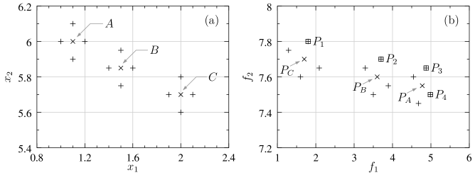
Figure 2: Illustration of local search for the optimisation problem given by Eq. 1. (a)  Points in decision space, (b) corresponding points in objective space. The original ND points, the points generated by local search, and the new ND points are marked with crosses, pluses, and squares, respectively.

Suppose the current ND set contains three points $A$, $B$, $C$ in Fig. 2 (a). The corresponding objective function values are shown by $P_{A}$, $P_{B}$, $P_{C}$ in Fig. 2 (b). Our goal is to improve the ND set using local search. To this end, we generate four neighbouring points centred around each existing solution, as shown in Fig. 2 (a). The $x_{1}$ and $x_{2}$ positions of the neighbours are given by

$$x_{1}^{\mathrm{new}}=x_{1}^{\mathrm{old}}\pm\Delta x_{1},~{}~{}x_{2}^{\mathrm{new}}=x_{2}^{\mathrm{old}}\pm\Delta x_{2}.$$ (2)

The corresponding neighbours in the objective space are shown in Fig. 2 (b). We now find the ND solutions from the entire set consisting of the old solutions and the newly generated solutions. The new ND set is made up of $P_{1}$, $P_{2}$, $P_{3}$, $P_{4}$ in Fig. 2 (b). Note that the ND set has improved in two ways: (a) The number of solutions has increased from 3 to 4, (b) The ND points in the new set dominate the old ND points – in this example, all of the old ND points ($P_{A}$, $P_{B}$, $P_{C}$).

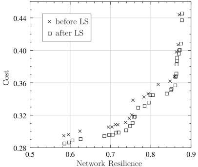
Figure 3: ND set for the BLA network at an early stage of the MOEA before and after applying local search (cost is in millions of USD).

It is important to evaluate the neighbours of each solution in the ND set first and then update the ND set by removing dominated solutions [25]. For example, in Fig. 2 (a), suppose we first evaluate the neighbours of $A$ and obtain two new ND points $P_{3}$ and $P_{4}$. If the ND set is updated at this stage, solution $B$ will get removed (since $P_{B}$ is dominated by $P_{3}$). As a consequence, the neighbours of $B$ will not get evaluated, and the ND solution $P_{2}$ will not be obtained. To avoid this situation in MOPSO+, we first prepare a list of all solutions whose neighbours are to be explored. Subsequently, we treat the members of this list one by one until the entire list is covered. The new solutions are then used to update the ND set.

For the WDS problems we are considering here, the decision variables are the pipe diameters. Each decision variable can take on values 1, 2, $\cdots$, $N_{\mathrm{dia}}$ (where $N_{\mathrm{dia}}$ is the number of possible diameters, see Table 1), with 1 corresponding to the smallest diameter, 2 to the next larger diameter, etc. For the BLA network, for example, there are 23 decision variables, each taking a value between 1 and 14. We consider two solutions to be neighbours if they differ by $\pm 1$ in one of the decision variables. In the BLA case, therefore, a general solution not lying on a decision space boundary would have $23\times 2\,$=$\,46$ neighbours. If there are $N^{\prime}$ solutions in the current ND set, we need to perform $46\times N^{\prime}$ function evaluations, each involving a call the the EPANET program for computation of cost and resilience. The results before and after local search are shown in Fig. 3 for the BLA network at an early stage of the MOEA. The improvement arising from local search can be clearly observed.

The above procedure is obviously expensive. One way to reduce the number of function evaluations is to keep track of points which have already been evaluated. For these points, it is not necessary to repeat function evaluation. However, comparison of a given point with a list of points (in the decision space) is also expensive if it is compared with each point in the list one by one. To make the comparison more efficient, we employ a tree structure to represent the ND set. An example is shown in Fig. 4. In this case, there are three decision variables $x_{1}$, $x_{2}$, $x_{3}$. Nodes at level $x_{k}$ are labeled by the $x_{k}$ values of the solutions. The path traced in checking if the solution $x_{1}\,$=$\,3$, $x_{2}\,$=$\,1$, $x_{3}\,$=$\,2$, is present in the ND set is shown with a thick grey line.

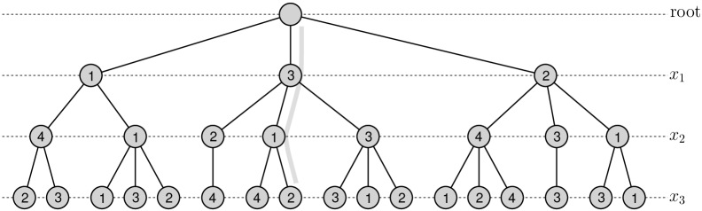
Figure 4: Tree structure used for storing solutions in the non-dominated set.

4 MOPSO+ algorithm

In this paper, we demonstrate the usefulness of a hybrid algorithm using the MOPSO algorithm along with local search for the WDS design problem. Several variations of the MOPSO algorithm have been reported (see [29],[30] for a review). Here, we use the MOPSO algorithm proposed by Coello [16], with some modifications.

The velocity update formula in MOPSO is similar to that used in single-objective PSO, and is given by

$${\bf{v}}_{i}(t)=W\,{\bf{v}}_{i}(t-1)+C_{1}r_{1}({\bf{x}}_{\mathrm{pbest}}^{i}-{\bf{x}}_{i}(t))+C_{2}r_{2}({\bf{x}}_{\mathrm{leader}}-{\bf{x}}_{i}(t)),$$ (3)

where $t$ denotes the PSO iteration number, ${\bf{x}}_{i}$ and ${\bf{v}}_{i}$ are the position and velocity of the $i^{\mathrm{th}}$ particle, respectively, and $r_{1}$ and $r_{2}$ are random numbers between 0 and 1. The algorithm parameters are $W$ (inertia weight), $C_{1}$ (cognitive learning factor), and $C_{2}$ (social learning factor). In this work, we have used $W\,$=$\,0.4$, $C_{1}\,$=$\,2$, $C_{2}\,$=$\,2$. It should be pointed out that, although the decision variables in the WSD benchmark problems considered here take on discrete values, they are treated as real numbers in the velocity and position update equations. In computing the particle fitness, each decision variable is converted to the nearest integer (which gives the pipe diameter index for the concerned pipe).

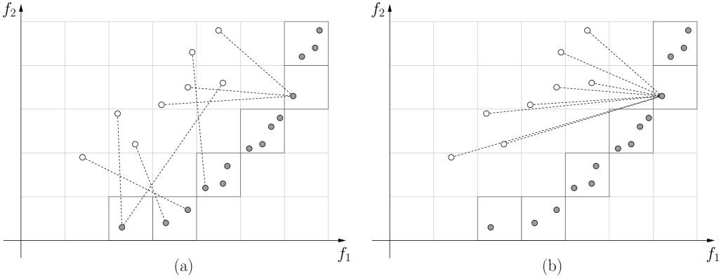
Figure 5: Illustration of leader selection procedure: (a) MOPSO algorithm [16], (b) MOPSO+ algorithm (this work). Hollow circles: PSO particles, filled circles: current ND solutions.

The MOPSO algorithm differs from the single-objective PSO algorithm in the computation of ${\bf{x}}_{\mathrm{pbest}}^{i}$ (the personal best position of the particle so far) and ${\bf{x}}_{\mathrm{leader}}$ (the position of the leader). In [16], ${\bf{x}}_{\mathrm{pbest}}^{i}$ is updated in every iteration by comparing its current position with the previous value of ${\bf{x}}_{\mathrm{pbest}}^{i}$. If the current position dominates, it replaces ${\bf{x}}_{\mathrm{pbest}}^{i}$. If it is non-dominated with respect to ${\bf{x}}_{\mathrm{pbest}}^{i}$, then one of them is selected randomly as the next ${\bf{x}}_{\mathrm{pbest}}^{i}$.

In MOPSO [16], assignment of ${\bf{x}}_{\mathrm{leader}}$ is made using the ND set stored in an external archive (repository). The objective space is divided into hypercubes, and each ND solution, depending on its position in the objective space, is assigned one of these hypercubes. For each particle, in each PSO iteration, a leader is selected from the archive giving preference to ND solutions which occupy less-crowded hypercubes. Roulette-wheel selection is used to first select a hypercube, and one of the ND solutions in that hypercube is picked randomly as the leader. This procedure helps to ensure that the ND solutions are well distributed in the objective space.

In addition, a mutation operator is used in [16] to enhance exploration of the search space in the beginning of the search. The mutation rate is made zero as the algorithm converges.

With this background, we now describe modifications made in the proposed MOPSO+ algorithm.

• Archive manipulation: The hypergrid approach used in [16] was modified in [31] to avoid changing of grid boundaries and for more efficient use of memory. This new approach, which uses a hypergrid with a fixed cell size and does not involve grid boundaries, is used in the MOPSO+ program.

• Leader selection: The leader selection process in MOPSO [16] is illustrated in Fig. 5 (a). In each PSO iteration, each particle is assigned one of the ND particles in the archive, preferring less crowded hypercubes. In MOPSO+, we continue to use the roulette-wheel selection procedure of the MOPSO algorithm. However, to intensify exploration of the less-crowded regions of the archive, we assign the same leader to all particles, as shown in Fig. 5 (b) and keep the same leader for $N_{\rm{leader}}^{\rm{const}}$ iterations.

• Mutation: In PSO, when the velocity and position update steps fail to generate new ND solutions, mutation can be useful [30]. In the context of the WDS benchmark problems, we have observed that there is an initial phase of MOPSO in which the ND set is improved relatively rapidly. However, beyond a certain point, the rate of generation of new solutions drops significantly. For this reason, different mutation schemes have been implemented in MOPSO+ (see Fig. 6).

  In the “constant” option, the mutation probability remains constant (a low value such as 0.01). In the “pulse” option, the probability is made non-zero only for $N_{\rm{mut}}$ iterations in the early stages and zero otherwise. In the “periodic” option, the probability is made non-zero for $N_{\rm{mut}}$ iterations in every $N_{\rm{period}}$ iterations, thus periodically encouraging enhanced exploration. The mutation process itself is common in the three cases and involves changing one of the decision variables of the particle randomly.

• Local search: The local search operation has been described in Sec. 3. We will refer to that procedure as a “unit local search” (ULS) step. In MOPSO+, local search is implemented as follows.

  • As seen in Sec. 3, a ULS step can lead to some improvement in the ND set. If it is applied again on the new ND set, further improvement is possible [25]. For this purpose, MOPSO+ allows the ULS to be repeated $N_{LS}^{\rm{max}}$ times at a given PSO iteration. If, after some ULS steps, it is found that no further generation of new ND solutions is taking place, the LS step is discontinued.

  • As explained in Sec. 3, local search is expensive, and it is not practical to perform it in every PSO iteration. In MOPSO+, therefore, LS is performed periodically instead of every iteration. Furthermore, it was observed in the context of the benchmark WDS problems that LS is more effective in the early stages. Based on this observation, a two-stage LS strategy is implemented. From iteration $N_{PSO}^{(1)}$ to $N_{PSO}^{(2)}$, LS is performed every $T_{1}$ iterations, and after $N_{PSO}^{(2)}$, it is performed every $T_{2}$ iterations.

5 Results for medium problems

In this section, we present results obtained with the MOPSO+ algorithm for the “medium” problems (MP) listed in Table 1. We first consider the HAN network to understand the effect of the various algorithm parameters. We then choose the set of parameters which gives the best performance for the HAN network and use it for the other three benchmark problems in the MP category, viz., the NYT, BLA, and GOY networks. We will refer to the ND sets reported in [16] as “UExeter PFs” and the ND sets given by MOPSO+ as the “MOPSO+ PFs.”

Table 3: Comparison of UExeter and MOPSO+ PFs for the HAN network for different MOPSO+ options.

MOPSO+	$N_{PSO}^{\mathrm{max}}$	UExeter (PF-A)					MOPSO+ (PF-B)					$N^{c}$
options		$N_{A}^{t}$	$N_{A}^{a}$	$N_{A}^{u}$	$N_{A}^{r}$	$N_{FE}^{\rm{net}}$	$N_{B}^{t}$	$N_{B}^{a}$	$N_{B}^{u}$	$N_{B}^{r}$	$N_{FE}^{\rm{net}}$
LS/Leadernew/Mperiodic	10,000	575	534	1	41	90 M	750	748	215	2	74.6 M	533
LS/Leaderold/Mperiodic	10,000	575	537	4	38	90 M	726	714	181	12	71.3 M	533
LS/Leadernew/Mnone	10,000	575	552	88	23	90 M	629	581	117	48	59.6 M	464
LS/Leadernew/Mconstant	10,000	575	536	13	39	90 M	721	703	180	18	69.1 M	523
LS/Leadernew/Mpulse	10,000	575	535	13	40	90 M	748	729	207	19	71.0 M	522
LSnone/Leadernew/Mperiodic	10,000	575	558	187	17	90 M	561	452	81	109	40.0 M	371
LSnone/Leadernew/Mperiodic	20,000	575	553	92	22	90 M	660	577	116	83	80.0 M	461

Table 3 shows the results (i.e., $N_{A}^{t}$, $N_{A}^{u}$, etc. as defined in Sec. 2) for the HAN network with $N_{p}\,$=$\,200$ (number of particles). For the first six rows of the table, the number of PSO iterations $N_{r}\,$=$\,10,000$ while for the last row, it is 20,000.

The MOPSO+ options mentioned in the first column have the following meaning.

• LS: Local search is performed with a period of 100 between $N_{PSO}\,$=$\,1,000$ and 5,000, and with a period of 1,000 thereafter. The parameter $N_{LS}^{\rm{max}}$ (see Sec. 3) is set to 50.

• Leader^new: The new leader assignment scheme (Fig. 5 (b)) is used with $N_{\rm{leader}}^{\rm{const}}\,$=$\,10$.

• Leader^old: The leader assignment scheme of [16] (Fig. 5 (a)) is used.

• M^none: No mutation is performed.

• M^constant: Constant mutation (Fig. 6 (a)) is performed with $p_{0}\,$=$\,0.02$.

• M^pulse: Pulse mutation (Fig. 6 (b)) is performed with $p_{0}\,$=$\,1$, $N_{\mathrm{mut}}\,$=$\,20$, starting with $N_{PSO}\,$=$\,1,000$.

• M^periodic: Periodic mutation (Fig. 6 (c)) is performed with $p_{0}\,$=$\,1$, $N_{\mathrm{mut}}\,$=$\,20$, $N_{\mathrm{mut}}^{\mathrm{period}}\,$=$\,1,000$, starting with $N_{PSO}\,$=$\,1,000$.

• LS^none: Local search is not used.

In each case, 20 independent runs of MOPSO+ were performed, and the total number of function evaluations (using the EPANET program) $N_{FE}^{\rm{net}}$ over all independent runs was recorded. We can make the following observations from Table 3.

• For each set of MOPSO+ options, a substantial number of new ND solutions (given by $N_{B}^{u}$) are found.

• Comparing the first two rows, we find that the new leader assignment scheme used in MOPSO+ gives a larger $N_{B}^{u}$. It also results in a smaller $N_{A}^{u}$, which is desirable, as explained in Sec. 3.

• Among the different mutation schemes (see rows 1, 3, 4, 5), the periodic scheme gives the best PF.

• Local search plays a very important role (see rows 1 and 6) in MOPSO+. Without LS, we see that a large number of UExeter solutions ($N_{A}^{u}\,$=$\,187$) are missed out by MOPSO+. Also, there is a substantial reduction (from 215 to 81) in the number of new solutions found by MOPSO+ when LS is not used.

• Although LS has improved the ND set, it has taken a larger number of function evaluations ($N_{FE}^{\rm{net}}\,$=$\,74.6\,$M with LS as against $N_{FE}^{\rm{net}}\,$=$\,40\,$M without LS, see rows 1 and 6). To make a fair comparison, we have run MOPSO+ without LS with a larger $N_{FE}^{\rm{net}}\,$=$\,80\,$M by doubling $N_{PSO}^{\mathrm{max}}$, the number of PSO iterations. In this situation (row 7), $N_{A}^{u}$ and $N_{B}^{u}$ are worse than row 1 which implies that improvement due to LS is not simply because of increased $N_{FE}^{\rm{net}}$.

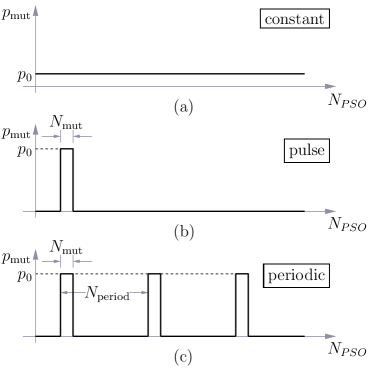
Figure 6: Mutation probability versus PSO iteration number for different mutation schemes implemented in MOPSO+.

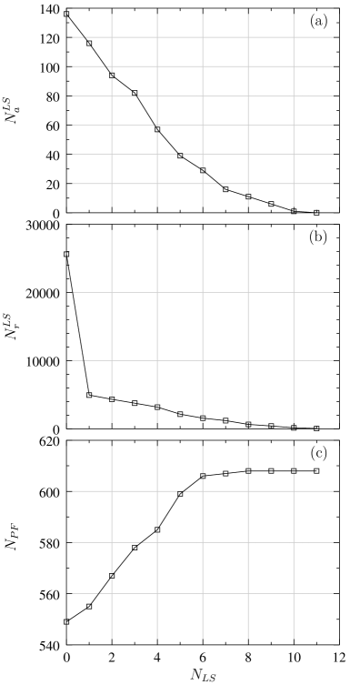
Figure 7: Illustration of the local search process at a specific PSO iteration ($N_{PSO}\,$=$\,1,100$) for the HAN network with algorithm parameters same as those for row 1 of Table 3. (a) Number of accepted solutions, (b) Number of rejected solutions, (c) Number of solutions in the ND set.

It is instructive to look at the LS process for one specific run for the first row of Table 3. At a given PSO iteration at an early stage ($N_{PSO}\,$=$\,1,100$), the number of accepted solutions ($N_{a}^{LS}$), the number of rejected solutions ($N_{r}^{LS}$), and the number of solutions in the updated ND set ($N_{PF}$) are plotted versus $N_{LS}$, the LS iteration number, in Figs. 7 (a)-(c). At the first LS iteration ($N_{LS}\,$=$\,0$), the number of solutions in the ND set is about 550, which means that there are $550\times 2\times 34$ (where 34 is the number of decision variables), i.e., 37,400 neighbours if all of the 550 points are interior. Some of these points would lie on the boundaries of the decision space, and they would have less than $2\times 34$ neighbours each. Nevertheless, it is clear that the number of solutions to be evaluated at the first LS iteration is rather large. Of these, only 138 solutions (Fig. 7 (a)) get accepted in the ND set. About 25,000 (Fig. 7 (b)) are found to be dominated by other solutions in the ND set and are therefore rejected.

During the first LS iteration (i.e., the ULS step described earlier), a list of all solutions being evaluated is prepared using the tree format shown in Fig. 4. In the subsequent LS iterations, the neighbours of the updated ND solutions are compared against this list, and only those not found in the list are evaluated. Therefore, a much smaller number of solutions need to be tried in the subsequent LS iterations. For example, for $N_{LS}\,$=$\,1$, only about 5,000 solutions need to be evaluated. This process continues until either $N_{LS}^{\rm{max}}$ iterations are completed or when an LS iteration fails to generate any new ND solutions. For the example shown in Fig. 7, the latter situation is reached (at $N_{LS}\,$=$\,11$). With each LS iteration, the ND set gets improved, and in this specific example, the number of solutions in the ND set also increases (Fig. 7 (c)) with each LS iteration.

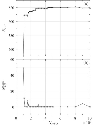
Figure 8: (a) Number of ND solutions ($N_{PF}$) and (b) number of total LS iterations ($N_{LS}^{\mathrm{total}}$) versus PSO iteration number for the HAN network with algorithm parameters same as those for row 1 of Table 3.

Fig. 8 (a) shows the variation of the size of the ND set ($N_{PF}$), and Fig. 8 (b) shows the total number of LS iterations tried ($N_{LS}^{\mathrm{total}}$) as the MOPSO+ algorithm proceeds. Note that, as mentioned earlier, the period of local search is low (100) up to $N_{PSO}\,$=$\,5,000$ and high (1,000) thereafter, and that is the reason for the larger density of data points up to $N_{PSO}\,$=$\,5,000$ in Fig. 8 (b). For the first LS step (at $N_{PSO}\,$=$\,1,000$), $N_{LS}^{\mathrm{total}}\,$=$\,N_{LS}^{\mathrm{max}}\,$=$\,50$. Beyond this point, generation of ND solutions due to LS slows down, and after about 2,000 PSO iterations, we see that $N_{LS}^{\mathrm{total}}$ mostly remains zero (which means only one LS iteration was tried which failed to produce new ND points). This points to a side benefit of using LS: it provides a necessary (but not sufficient) condition for convergence of an MOEA. If LS yields additional ND points, we can say that the MOEA has not converged.

Table 4: Comparison of UExeter and MOPSO+ PFs for different values of $N_{p}$ (number of particles), $N_{PSO}^{\mathrm{max}}$ (number of PSO iterations), and $N_{r}$ (number of independent runs) for the NYT network.

MOPSO+ options			UExeter (PF-A)					MOPSO+ (PF-B)					$N^{c}$
$N_{p}$	$N_{PSO}^{\mathrm{max}}$	$N_{r}$	$N_{A}^{t}$	$N_{A}^{a}$	$N_{A}^{u}$	$N_{A}^{r}$	$N_{FE}^{\mathrm{net}}$	$N_{B}^{t}$	$N_{B}^{a}$	$N_{B}^{u}$	$N_{B}^{r}$	$N_{FE}^{\mathrm{net}}$
200	20,000	30	627	599	20	28	90 M	648	639	60	9	150.7 M	579
300	20,000	30	627	597	28	30	90 M	670	630	61	40	211.3 M	569
100	60,000	10	627	596	25	31	90 M	655	635	64	20	76.7 M	571
100	60,000	17	627	595	4	32	90 M	661	656	65	5	130.3 M	591

Table 5: Comparison of UExeter and MOPSO+ PFs for the four MP networks described in [16]. The MOPSO+ algorithm parameters are the same as row 1 of Table 3.

Network	MOPSO+ options			UExeter (PF-A)					MOPSO+ (PF-B)					$N^{c}$
	$N_{p}$	$N_{PSO}^{\mathrm{max}}$	$N_{r}$	$N_{A}^{t}$	$N_{A}^{a}$	$N_{A}^{u}$	$N_{A}^{r}$	$N_{FE}^{\mathrm{net}}$	$N_{B}^{t}$	$N_{B}^{a}$	$N_{B}^{u}$	$N_{B}^{r}$	$N_{FE}^{\mathrm{net}}$
NYT	100	60,000	17	627	595	4	32	90 M	661	656	65	5	130.3 M	591
BLA	200	10,000	10	901	849	0	52	90 M	1045	1045	196	0	44.1 M	849
HAN	200	10,000	20	575	534	1	41	90 M	750	748	215	2	74.6 M	533
GOY	100	20,000	10	489	444	3	45	90 M	571	570	129	1	37.9 M	441

We now use the MOPSO+ algorithm parameters which have been found to work well for the HAN problem (option LS/Leader^new/M^periodic in Table 3) for optimisation of the other medium problems described in [16], viz., the NYT, BLA, and GOY networks. The results for the NYT network are shown in Table 4. We observe that the $N_{B}^{u}$ values are comparable in the four cases listed in the table. However, for $N_{p}\,$=$\,100$, $N_{PSO}^{\mathrm{max}}\,$=$\,60,000$, and $N_{r}\,$=$\,17$, $N_{A}^{u}$ is substantially lower than the other three cases.

Comparing rows 1 and 2 of the table, we conclude that increasing the number of particles is not necessarily beneficial, which was also pointed out in [7] for other MOEAs. A systematic study of the effect of $N_{p}$ and $N_{PSO}^{\mathrm{max}}$ on the performance of MOPSO+ has not been carried out in this work. Instead, we present the results obtained after limited experimentation with these parameters.

Table 5 shows the results for the four MP benchmark problems described in [16]. In each case, a substantial number of new ND solutions ($N_{B}^{u}$) have been found by MOPSO+. Furthermore, almost all ND solutions in the UExeter PFs are covered by MOPSO+ (see the $N_{A}^{u}$ column in the table). The improvement in the PFs have been obtained with a smaller $N_{FE}^{\mathrm{net}}$ for three networks and with a larger $N_{FE}^{\mathrm{net}}$ for the NYT network. These results overall point to the usefulness of the MOPSO+ approach for the WDS design problem.

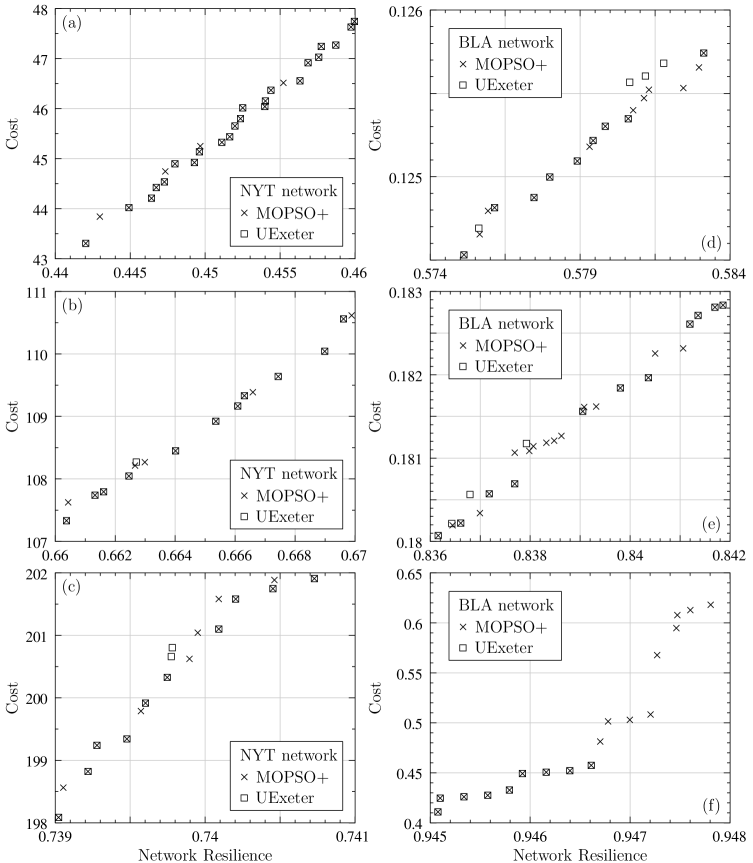
Figure 9: UExeter [15] and MOPSO+ ND sets for the NYT and BLA networks for different ranges of network resilience.

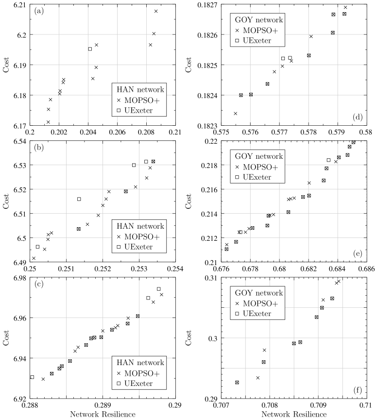
Figure 10: UExeter [15] and MOPSO+ ND sets for the HAN and GOY networks for different ranges of network resilience.

Figs. 9 (a)-(f) and 10 (a)-(f) show expanded plots of the UExeter and MOPSO+ PFs. It can be seen that some of the MOPSO+ solutions dominate some of the UExeter solutions.

Table 6: Objective function and decision variable values for a few solutions of Fig. 9 (d) obtained by MOPSO+ for the BLA network.

	sol. 1	sol. 2	sol. 3	sol. 4	sol. 5	sol. 6	sol. 7
Resilience	0.57931	0.57943	0.57984	0.58060	0.58077	0.58113	0.58129
Cost	0.12518	0.12522	0.12530	0.12535	0.12540	0.12547	0.12552
$d_{1}$	254.0	254.0	254.0	254.0	254.0	254.0	254.0
$d_{2}$	101.6	101.6	101.6	101.6	101.6	101.6	101.6
$d_{3}$	203.2	203.2	203.2	203.2	203.2	203.2	203.2
$d_{4}$	203.2	203.2	203.2	203.2	203.2	203.2	203.2
$d_{5}$	152.4	152.4	152.4	152.4	152.4	152.4	152.4
$d_{6}$	152.4	152.4	152.4	152.4	152.4	152.4	152.4
$d_{7}$	152.4	152.4	152.4	152.4	152.4	152.4	152.4
$d_{8}$	25.4	25.4	25.4	25.4	25.4	25.4	25.4
$d_{9}$	152.4	152.4	152.4	152.4	152.4	152.4	152.4
$d_{10}$	101.6	101.6	101.6	101.6	101.6	101.6	101.6
$d_{11}$	101.6	76.2	101.6	76.2	76.2	76.2	76.2
$d_{12}$	152.4	152.4	152.4	152.4	152.4	152.4	152.4
$d_{13}$	152.4	152.4	152.4	152.4	152.4	152.4	152.4
$d_{14}$	152.4	152.4	152.4	152.4	152.4	152.4	152.4
$d_{15}$	76.2	101.6	101.6	76.2	76.2	101.6	101.6
$d_{16}$	50.8	50.8	50.8	50.8	50.8	50.8	50.8
$d_{17}$	50.8	50.8	50.8	50.8	50.8	50.8	50.8
$d_{18}$	76.2	50.8	76.2	25.4	76.2	25.4	76.2
$d_{19}$	25.4	25.4	25.4	25.4	25.4	25.4	25.4
$d_{20}$	101.6	101.6	101.6	152.4	101.6	152.4	101.6
$d_{21}$	25.4	25.4	25.4	25.4	25.4	25.4	25.4
$d_{22}$	152.4	152.4	152.4	152.4	152.4	152.4	152.4
$d_{23}$	101.6	152.4	101.6	101.6	152.4	101.6	152.4

Even though many of the unique MOPSO+ solutions (i.e., solutions present in the MOPSO+ PFs but not in the UExeter PFs) are close in the objective space to the previously known UExeter solutions, they can differ substantially in the decision space. For example, some of the ND solutions obtained by MOPSO+ for the BLA network are shown in Table 6. Of these, solutions 2, 3, 4 are also present in the UExeter PF while solutions 1, 5, 6, 7 are new. Although the cost and resilience values for solutions 1 and 2 differ only in the fourth decimal place, we observe that these two solutions vary substantially in the decision space – four diameter values, viz., $d_{11}$, $d_{15}$, $d_{18}$, $d_{23}$, are different. This could have important implications in practice because of non-technical issues such as land acquisition, and a wider choice of ND solutions may well open up previously unknown options for the DM. The metrics proposed in Sec. 2 therefore seem to be more attractive from a practical perspective than metrics such as average cost, lowest cost, standard deviation, or spread.

6 Results for an intermediate problem

As seen in Sec. 3, local search is an expensive step, and with a large number of decision variables (in our context, the number of pipes) involved in the networks of IP and LP categories in [7], the repeated ULS procedure described for the MP category (see Sec. 4) can become prohibitively expensive. In this section, we will consider one of the IPs, the PES network (see Table 1). Since there are 99 decision variables, local search around one solution involves $99\times 2\,$=$\,198$ function evaluations. As we shall see, the ND set for this network is much larger than the MP networks, making even one unit local search step involving evaluation of all neighbours of all solutions in the ND set consume significant computation time.

In view of the above difficulty, the ND set is only partially explored during local search (see [22],[27]), and only one ULS step is performed. In particular, $N_{ND}^{\mathrm{max}}$ solutions from the current ND set are randomly selected, and all neighbours of the selected solutions are evaluated. Apart from this change, other algorithm details remain the same as before.

For the PES problem, 10 independent runs of MOPSO+ were performed with $N_{p}\,$=$\,200$ and $N_{PSO}\,$=$\,1,000,000$. Periodic mutation was employed, with $p_{0}\,$=$\,1$, $N_{\mathrm{mut}}\,$=$\,50$, $N_{\mathrm{mut}}^{\mathrm{period}}\,$=$\,1,000$, starting with $N_{PSO}\,$=$\,1,000$. The new scheme for finding the leader (see Sec. 4) is used, with $N_{\rm{leader}}^{\rm{const}}\,$=$\,10$. Local search was performed with a period of 1,000 between $N_{PSO}\,$=$\,1,000$ and 10,000, and with a period of 10,000 thereafter. $N_{ND}^{\mathrm{max}}$ was set to 200, which means only 200 solutions from the current ND set are randomly picked for any LS step.

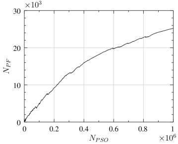
Figure 11: Number of ND solutions ($N_{PF}$) versus PSO iteration number for the PES network.

Fig. 11 shows $N_{PF}$ (the number of ND solutions) versus PSO iteration number for one independent run. A much larger $N_{PF}$ (about 25,000) is obtained for this network. Note that, in contrast to Fig. 8 for the HAN network, $N_{PF}$ has not saturated in this case, indicating that $N_{PF}$ may increase further with additional PSO iterations.

Table 7: Comparison of UExeter and MOPSO+ PFs for different values of $N_{r}$ (number of independent runs) for the PES network.

$N_{r}$	UExeter (PF-A)					MOPSO+ (PF-B)					$N^{c}$
	$N_{A}^{t}$	$N_{A}^{a}$	$N_{A}^{u}$	$N_{A}^{r}$	$N_{FE}^{\rm{net}}$	$N_{B}^{t}$	$N_{B}^{a}$	$N_{B}^{u}$	$N_{B}^{r}$	$N_{FE}^{\rm{net}}$
1	782	307	292	475	150 M	21,536	12,161	12,146	9,375	269 M	15
2	782	190	175	592	150 M	20,736	14,856	14,841	5,880	538 M	15
3	782	167	152	615	150 M	22,949	20,081	20,066	2,868	808 M	15
4	782	166	152	616	150 M	22,962	20,094	20,080	2,868	1,077 M	14
5	782	39	22	743	150 M	23,267	23,168	23,151	99	1,348 M	17
6	782	37	19	745	150 M	24,643	24,547	24,529	96	1,619 M	18
7	782	36	19	746	150 M	25,607	25,510	25,493	97	1,889 M	17
8	782	36	19	746	150 M	26,145	26,048	26,031	97	2,160 M	17
9	782	35	18	747	150 M	26,488	26,399	26,382	89	2,431 M	17
10	782	35	18	747	150 M	30,267	30,178	30,161	89	2,703 M	17

Table 7 shows the effect of $N_{r}$ (the number of independent runs) on the performance of MOPSO+. With a single run, $N_{B}^{u}\,$=$\,12,146$ new solutions are generated. However, $N_{A}^{u}\,$=$\,292$ solutions from the UExeter PF are missed out by MOPSO+. The number of function evaluations for this run is 269 M out of which $N_{p}\times N_{r}\,$=$\,200$ M are due to the PSO part and 69 M are due to local search. This value of $N_{FE}^{\rm{net}}$ is already larger than the UExeter value of 150 M. As more independent runs are performed, $N_{FE}^{\rm{net}}$ increases proportionately. However, the number of additional ND solutions increases with $N_{r}$, and the number of UExeter ND solutions ($N_{A}^{u}$) missed by MOPSO+ decreases, both factors being favourable. For ten runs, $N_{FE}^{\rm{net}}$ for MOPSO+ is about 18 times larger than UExeter. Considering the large number of new ND solutions (about 38 times larger than UExeter), the additional computational effort seems worthwhile.

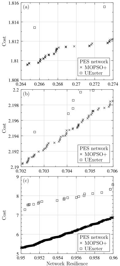
Figure 12: UExeter [15] and MOPSO+ ND sets for the PES network for different ranges of network resilience.

Some of the ND solutions obtained by MOPSO+ are shown in Figs. 12 (a)-(c), along with UExeter solutions. It can be seen that the density of solutions obtained by MOPSO+ is larger. Also, for some values of network resilience (see Fig. 12 (c)), the cost for some of the MOPSO+ solutions is lower by as much as 25 %.

7 Conclusions

In summary, a hybrid algorithm (MOPSO+) comprising a multi-objective particle swarm optimisation algorithm and local search is presented for water distribution system design. Four medium and one intermediate benchmark networks are considered, and for each of them, a significant number of new non-dominated solutions have been obtained using the proposed algorithm, thus improving the best-known Pareto fronts for these problems. For medium networks, the total number of function evaluations for MOPSO+ was of the same order as in [7]. For the intermediate network considered here, although the total $N_{FE}$ was much larger (18 times) for MOPSO+, the large number of new solutions generated by MOPSO+ justifies the additional computational effort.

Based on the results presented here, MOPSO+ seems to be an attractive option for WDS design. Some important issues for future research in this area are listed below.

• Performance of MOPSO+ for other networks in the IP and LP category needs to be investigated.

• A unified set of algorithmic parameters for all problems of a particular complexity (MP, IP, LP) is desirable. More work is required to explore this possibility.

• The LS mechanism introduced here can be applied to other multi-objective optimisation problems with discrete decision variables.

• In order to speed up convergence, techniques such as reduction of search space [8], high-quality initial population [11] could be combined with the MOPSO+ algorithm.

References

- [1] R. Farmani, G. A. Walters, and D. A. Savic, “Trade-off between total cost and reliability for anytown water distribution network,” Journal of Water Resources Planning and Management, vol. 131, no. 3, pp. 161–171, 2005.
- [2] M. J. Reddy and D. N. Kumar, “An efficient multi-objective optimization algorithm based on swarm intelligence for engineering design,” Engineering Optimization, vol. 39, no. 1, pp. 49–68, 2007.
- [3] M. S. Kadu, R. Gupta, and P. R. Bhave, “Optimal design of water networks using a modified genetic algorithm with reduction in search space,” Journal of Water Resources Planning and Management, vol. 134, no. 2, pp. 147–160, 2008.
- [4] I. Montalvo, J. Izquierdo, S. Schwarze, and R. Pérez-García, “Multi-objective particle swarm optimization applied to water distribution systems design: an approach with human interaction,” Mathematical and Computer Modelling, vol. 52, no. 7-8, pp. 1219–1227, 2010.
- [5] D. N. Raad, “Multi-objective optimisation of water distribution systems design using metaheuristics,” Ph.D. dissertation, Stellenbosch: University of Stellenbosch, 2011.
- [6] M. Ahmadi, M. Arabi, D. L. Hoag, and B. A. Engel, “A mixed discrete-continuous variable multiobjective genetic algorithm for targeted implementation of nonpoint source pollution control practices,” Water Resources Research, vol. 49, no. 12, pp. 8344–8356, 2013.
- [7] Q. Wang, M. Guidolin, D. Savic, and Z. Kapelan, “Two-objective design of benchmark problems of a water distribution system via MOEAs: Towards the best-known approximation of the true pareto front,” Journal of Water Resources Planning and Management, vol. 141, no. 3, p. 04014060, 2014.
- [8] E. Barlow and T. T. Tanyimboh, “Multiobjective memetic algorithm applied to the optimisation of water distribution systems,” Water resources management, vol. 28, no. 8, pp. 2229–2242, 2014.
- [9] M. Morley and C. Tricarico, “A comparison of population-based optimization techniques for water distribution system expansion and operation,” Procedia Engineering, vol. 89, pp. 13–20, 2014.
- [10] D. Mora-Melia, P. L. Iglesias-Rey, F. J. Martinez-Solano, and P. Ballesteros-Pérez, “Efficiency of evolutionary algorithms in water network pipe sizing,” Water resources management, vol. 29, no. 13, pp. 4817–4831, 2015.
- [11] W. Bi, G. C. Dandy, and H. R. Maier, “Use of domain knowledge to increase the convergence rate of evolutionary algorithms for optimizing the cost and resilience of water distribution systems,” Journal of Water Resources Planning and Management, vol. 142, no. 9, p. 04016027, 2016.
- [12] N. Moosavian and B. Lence, “Nondominated sorting differential evolution algorithms for multiobjective optimization of water distribution systems,” Journal of Water Resources Planning and Management, vol. 143, no. 4, p. 04016082, 2016.
- [13] F. Zheng, A. C. Zecchin, J. P. Newman, H. R. Maier, and G. C. Dandy, “An adaptive convergence-trajectory controlled ant colony optimization algorithm with application to water distribution system design problems,” IEEE Transactions on Evolutionary Computation, vol. 21, no. 5, pp. 773–791, 2017.
- [14] L. A. Rossman et al., “EPANET 2: Users Manual,” 2000.
- [15] “Centre for water systems.” [Online]. Available: http://emps.exeter.ac.uk/engineering/research/cws/resources/benchmarks/design-resiliance-pareto-fronts/
- [16] C. A. C. Coello, G. T. Pulido, and M. S. Lechuga, “Handling multiple objectives with particle swarm optimization,” IEEE Trans. Evol. Comput., vol. 8, no. 3, pp. 256–279, 2004.
- [17] K. Deb, Multi-objective Optimization Using Evolutionary Algorithms. Chichester: J. Wiley and Sons, Ltd., 2009.
- [18] H. Ishibuchi and T. Yoshida, “Hybrid evolutionary multi-objective optimization algorithms.” in HIS, 2002, pp. 163–172.
- [19] J. Knowles and D. Corne, “Memetic algorithms for multiobjective optimization: issues, methods and prospects,” in Recent advances in memetic algorithms. Springer, 2005, pp. 313–352.
- [20] K. Sindhya, A. Sinha, K. Deb, and K. Miettinen, “Local search based evolutionary multi-objective optimization algorithm for constrained and unconstrained problems,” in 2009 IEEE Congress on Evolutionary Computation. IEEE, 2009, pp. 2919–2926.
- [21] A. A. Mousa, M. A. El-Shorbagy, and W. F. Abd-El-Wahed, “Local search based hybrid particle swarm optimization algorithm for multiobjective optimization,” Swarm and Evolutionary Computation, vol. 3, pp. 1–14, 2012.
- [22] A. Liefooghe, J. Humeau, S. Mesmoudi, L. Jourdan, and E. Talbi, “On dominance-based multiobjective local search: design, implementation and experimental analysis on scheduling and traveling salesman problems,” Journal of Heuristics, vol. 18, no. 2, pp. 317–352, 2012.
- [23] L. J. Dubois-Lacoste, M. López-Ibánez, and T. Stützle, “Combining two search paradigms for multi-objective optimization: Two-phase and pareto local search,” in Hybrid Metaheuristics. Springer, 2013, pp. 97–117.
- [24] M. Inja, C. Kooijman, M. de Waard, D. M. Roijers, and S. Whiteson, “Queued pareto local search for multi-objective optimization,” in International Conference on Parallel Problem Solving from Nature. Springer, 2014, pp. 589–599.
- [25] O. Maler and A. Srivastav, “Double archive pareto local search,” in 2016 IEEE Symposium Series on Computational Intelligence (SSCI). IEEE, 2016, pp. 1–7.
- [26] I. B. Mansour, I. Alaya, and M. Tagina, “Chebyshev-based iterated local search for multi-objective optimization,” in 2017 13th IEEE International Conference on Intelligent Computer Communication and Processing (ICCP). IEEE, 2017, pp. 163–170.
- [27] A. Jaszkiewicz, “Many-objective pareto local search,” European Journal of Operational Research, vol. 271, no. 3, pp. 1001–1013, 2018.
- [28] H. Kita, Y. Yabumoto, N. Mori, and Y. Nishikawa, “Multi-objective optimization by means of the thermodynamical genetic algorithm,” in International Conference on Parallel Problem Solving from Nature. Springer, 1996, pp. 504–512.
- [29] M. R. Sierra and C. A. C. Coello, “Improving PSO-based multi-objective optimization using crowding, mutation and -dominance,” in International Conference on Evolutionary Multi-Criterion Optimization. Springer, 2005, pp. 505–519.
- [30] K. E. Parsopoulos and M. N. Vrahatis, “Multi-objective particles swarm optimization approaches,” in Multi-objective optimization in computational intelligence: Theory and practice. IGI global, 2008, pp. 20–42.
- [31] M. B. Patil, “Using external archive for improved performance in multi-objective optimization,” submitted to Sādhanā.