Microscopic modelling of general time-dependent quantum Markov processes

Abstract

Master equations are typically adopted to describe the dynamics of open quantum systems. Such equations are either in integro-differential or in time-local form, with the latter class more frequently adopted due to the simpler numerical methods developed to obtain the corresponding solution. Here we show that any time-local master equation with positive rates in the generator, i.e. any CP-divisible quantum process, admits a microscopic model whose reduced dynamics is well described by the given equation.

Introduction.

In the theory of open quantum systems, master equations are widely adopted to describe the reduced dynamics. Such equations are typically derived from the full system-environment evolution via projection operator techniques, once an average over the environmental degrees of freedom is performed, and can be divided in two categories: integro-differential and time-local equations, respectively called Nakajima-Zwanzig and time-convolutionless master equations Breuer and Petruccione (2002); Nakajima (1958); Zwanzig (1960); Uchiyama and Shibata (1999); Breuer et al. (2006); Breuer (2007). Recently, various results have been obtained for the characterization of memory kernels leading to well-defined integro-differential quantum evolution equations Budini (2006); Breuer and Vacchini (2008); Vacchini (2013); Chruscinski and Kossakowski (2016); Vacchini (2016); Chruscinski and Kossakowski (2017), also pointing to connection with microscopic models Budini (2013); Lorenzo et al. (2017). However, the numerical implementation of integro-differential equations remains quite demanding Montoya-Castillo and Reichman (2016, 2017), so that time-convolutionless master equations often provide a more convenient approach. Moreover, in recent years such master equations also attracted a lot of interest because of their wide use in studying quantum non-Markovianity Breuer (2012); Rivas et al. (2014); Breuer et al. (2016). In fact, if one considers master equations with the same operator structure as the so-called Gorini-Kossakowski-Sudarshan-Lindblad generator Gorini et al. (1976); Lindblad (1976), which warrants hermiticity and trace preservation of the statistical operator, the relationship between the rates and the Lindblad operators allows to assess the divisibility character of the time evolution. Namely, whether the evolution map can be written as composition of maps referring to arbitrary intermediate time intervals. In particular, if the time evolution can be expressed as a composition of completely positive maps, the dynamics is said to be CP-divisible Breuer (2012); Breuer et al. (2016). In accordance with different recently proposed definitions and measures of quantum non-Markovianity, this divisibility enables a characterization of quantum memory effects, which are absent in the case of a CP-divisible dynamics Breuer et al. (2009); Rivas et al. (2010); Chruscinski et al. (2011); Wißmann et al. (2015); Amato et al. (2018). The solutions of time-convolutionless master equations characterized by positive rates in the generator, besides describing a well-defined evolution equation, do provide CP-divisible time evolutions Breuer (2012); Breuer et al. (2016). Nonetheless, master equations are not always derived from an underlying Hamiltonian model, they are often rather adopted to describe phenomenologically the non unitary dynamics of open quantum systems. It is hence an important task to clarify whether or not such equations actually correspond to a well-defined physical model.

The goal of this work is indeed to show that a system-environment interaction Hamiltonian can always be associated to any CP-divisible master equation, so that the reduced dynamics of the open system is described by the given equation. This is obtained considering the interaction of the system with multiple independent bosonic baths, truncated to the Born approximation, in the limit of infinite spectral densities bandwidth and assuring that there is no contribution to the two-time environmental correlation function due to negative frequencies components of the spectral density. This result shows that Markovian master equations are always connected to a modelling via the introduction of a bosonic environment and a suitable system-environment interaction Hamiltonian, for which they give an accurate description of the reduced dynamics, once some approximation, like weak-coupling and separation of relevant time-scales between system and environment, are adopted. Our work further opens the way to considering actual physical models in which such microscopic interaction can be realized.

Given an open quantum system $S$, with associated Hilbert space $\mathcal{H}_{S}$ such that $\textrm{dim}\mathcal{H}_{S}=n$, it is possible to describe its non unitary dynamics via the following time-convolutionless master equation

$$\frac{\textrm{d}}{\textrm{d}t}\rho_{S}(t)=-\frac{i}{\hbar}[H_{S}(t),\rho_{S}(t)]$$ (1)

$$\,+\!\sum_{k=1}^{n^{2}-1}\gamma_{k}(t)\left[A_{k}(t)\rho_{S}(t)A_{k}^{\dagger}(t)-\frac{1}{2}\{A_{k}^{\dagger}(t)A_{k}(t),\rho_{S}(t)\}\right],$$

where $\{A_{k}(t)\}_{k}$ are the so-called Lindblad operators and the real coefficients $\gamma_{k}(t)$ are called rates. If all rates are positive for $t\geq 0$, the associated quantum process is CP-divisible, according to the definition given above, that is, it gives rise to an evolution map that can be expressed as the composition of completely positive maps over any subdivision of the overall evolution time Breuer (2012); Breuer et al. (2016). In particular, positivity of the rates guarantees complete positivity of the reduced dynamics.

The main result of this contribution is to present a microscopic model, whose reduced dynamics is described, in a suitable limit, by a master equation of the form (1).

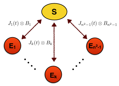
Figure 1: Schematic representation of the considered microscopic model, in which the system $S$ interacts with $n^{2}-1$ independent bosonic environments $E_{k}$, each corresponding to a dissipation channel in the master equation. The coupling is given through the dressed Lindblad operators $J_{k}(t)=\sqrt{{\gamma_{k}(t)}/{\gamma_{0}}}A_{k}(t)$ of Eq. (7) and the combination of field operators $B_{k}$ as given in Eq. (8).

Microscopic model.

We let the system $S$ interact with independent bosonic baths $E_{k}$, as depicted in Fig. 1, considering as an Ansatz the following total system-environment Hamiltonian

$$H(t)=\textrm{ }H_{S}(t)+H_{E}+H_{\textrm{int}}(t),$$ (2)

with $H_{S}(t)$ the Hamiltonian appearing in the commutator term in Eq. (1), while $H_{E}$ is the free Hamiltonian of the independent bosonic baths, so that

$$H_{E}=\textrm{ }\sum_{k=1}^{n^{2}-1}H_{E_{k}}$$ (3)

with

$$H_{E_{k}}=\sum_{\mu}\hbar(\omega_{k,\mu}-\omega_{0})b^{\dagger}_{k,\mu}b_{k,\mu},$$ (4)

where $b_{k,\mu}$ and $b^{\dagger}_{k,\mu}$ denote creation and annihilation bosonic operators satisfying the canonical commutation relations

$$[b_{k,\mu},b_{k^{\prime},\nu}]=[b^{\dagger}_{k,\mu},b^{\dagger}_{k^{\prime},\nu}]=0,\ [b_{k,\mu},b^{\dagger}_{k^{\prime},\nu}]=\delta_{kk^{\prime}}\delta_{\mu\nu},$$ (5)

and the associated frequencies are taken with respect to a reference frequency $\omega_{0}$, resonant with the system Gardiner and Zoller (2000). The interaction Hamiltonian is taken to be of the form

$$H_{\textrm{int}}(t)=\sum_{k=1}^{n^{2}-1}[J_{k}(t)\otimes B^{\dagger}_{k}+J_{k}^{\dagger}(t)\otimes B_{k}],$$ (6)

where the system operators $\{J_{k}(t)\}_{k}$ appearing in the coupling term are related to the original Lindblad operators according to

$$J_{k}(t)=\sqrt{{\gamma_{k}(t)}/{\gamma_{0}}}A_{k}(t),$$ (7)

where thanks to their positivity the rates, renormalized to a reference rate $\gamma_{0}$ which fixes the interaction strength, have been absorbed in the coupling operators. Note in particular that we do not put any constraint on the coupling strength, we only require that the rates $\gamma_{k}(t)$ are bounded functions of $t$ within the considered time interval and that the Lindblad operators $A_{k}(t)$ are bounded. The environmental coupling operators are instead given by

$$B_{k}=\sum_{\mu}g_{k,\mu}b_{k,\mu},$$ (8)

with $g_{k,\mu}$ coupling constants. The operators $J_{k}(t)$ are thus dimensionless, while $B_{k}(t)$ have the dimension of an inverse of time in units such that $\hbar=1$. We now move to the interaction picture with respect to the free Hamiltonian by means of the unitary transformation

$$V(t) =T_{\leftarrow}\exp\left\{-i\int_{0}^{t}\textrm{d}\tau\textrm{ }[H_{S}(\tau)+H_{E}]\right\}$$ (9)

$$={T_{\leftarrow}}\exp\left\{-i\int_{0}^{t}\textrm{d}\tau\textrm{ }H_{S}(\tau)\right\}\otimes\exp\left\{-iH_{E}t\right\},$$

which can be written $V(t)={V}_{S}(t)\otimes{V}_{E}(t)$, since $[H_{S}(t),H_{E}]=0$, and where $T_{\leftarrow}$ denotes operator time-ordering. Finally, the interaction Hamiltonian becomes

$$\tilde{H}_{\textrm{int}}(t)=\sum_{k=1}^{n^{2}-1}\left[\tilde{J}_{k}(t)\otimes\tilde{B}^{\dagger}_{k}(t)+\tilde{J}_{k}^{\dagger}(t)\otimes\tilde{B}_{k}(t)\right],$$ (10)

where the operators in the interaction picture are indicated by a tilde, so that $\tilde{J}_{k}(t)={V}^{\dagger}_{S}(t)J_{k}(t){V}_{S}(t)$ together with $\tilde{B}_{k}(t)={V}^{\dagger}_{E}(t)B_{k}{V}_{E}(t)$ which, exploiting Eq. (5), takes the form

$$\tilde{B}_{k}(t)=\sum_{\mu}g_{k,\mu}e^{-i(\omega_{k,\mu}-\omega_{0})t}b_{k,\mu}.$$ (11)

The exact evolution of the composite system in the interaction picture is thus described by the von Neumann equation

$$\frac{\textrm{d}}{\textrm{d}t}\tilde{\rho}(t)=-i\left[\tilde{H}_{\textrm{int}}(t),\tilde{\rho}(t)\right]\equiv\mathcal{L}(t)\tilde{\rho}(t),$$ (12)

and in the case of a factorized initial condition

$$\rho(0)=\rho_{S}(0)\otimes\sigma_{E}$$ (13)

warrants complete positivity of the reduced dynamics. The state of the environment $\sigma_{E}$ is taken to be the tensor product of zero temperature states for each bosonic bath, namely $\sigma_{E}=\bigotimes_{k=1}^{n^{2}-1}\sigma_{E_{k}}$ where

$$\sigma_{E_{k}}={\left|0\right\rangle\left\langle 0\right|}_{E_{k}},$$ (14)

with $b_{k,\mu}{\left|0\right\rangle}_{E_{k}}=0\ \forall\mu$.

Time-local master equation.

We now use the projection operator technique to derive a time-convolutionless master equation for the reduced dynamics Breuer and Petruccione (2002). To this aim, we consider a standard projection superoperator acting on a generic state $\omega$ of the total system as

$$\mathcal{P}\omega=\operatorname{Tr}_{E}\omega\otimes\sigma_{E},$$ (15)

with $\sigma_{E}$ the state of the environment appearing in the initial condition (13), so that in particular $\mathcal{P}\left[\rho(0)\right]=\rho(0)$. Using the Born approximation, namely considering terms up to the second order in the interaction Hamiltonian, starting from Eq. (12) one obtains

$$\frac{\textrm{d}}{\textrm{d}t}\mathcal{P}\tilde{\rho}(t)=\int_{0}^{t}\textrm{d}s\textrm{ }\mathcal{PL}(t)\mathcal{L}(s)\mathcal{P}\tilde{\rho}(t).$$ (16)

Tracing over the degrees of freedom of the environment, by means of a change of integration variable, one easily obtains the master equation

$$\frac{\textrm{d}}{\textrm{d}t}\tilde{\rho}_{S}(t)=-\int_{0}^{t}\textrm{d}\tau\operatorname{Tr}_{E}[\tilde{H}_{\textrm{int}}(t),[\tilde{H}_{\textrm{int}}(t-\tau),\tilde{\rho}_{S}(t)\otimes\sigma_{E}]],$$ (17)

which is sometimes called Redfield equation. We further expand the commutators and use the identities, valid $\forall\ i,k=1,...,n^{2}-1$ and $\forall\ t,s\geq 0$

$$\operatorname{Tr}_{E}\{\tilde{B}_{i}(t)\tilde{B}_{k}(s)\sigma_{E}\} =\operatorname{Tr}_{E}\{\tilde{B}^{\dagger}_{i}(t)\tilde{B}^{\dagger}_{k}(s)\sigma_{E}\}=0,$$ (18)

$$\operatorname{Tr}_{E}\{\tilde{B}^{\dagger}_{i}(t)\tilde{B}_{k}(s)\sigma_{E}\} =0,$$

together with

$$\operatorname{Tr}_{E}\{\tilde{B}_{i}(t)\tilde{B}^{\dagger}_{k}(s)\sigma_{E}\}=0$$ (19)

for $i\not=k$. The only nontrivial two-time correlation function is thus given by

$$\operatorname{Tr}_{E}\{\tilde{B}_{k}(t)\tilde{B}^{\dagger}_{k}(s)\sigma_{E}\} =\operatorname{Tr}_{E_{k}}\{\tilde{B}_{k}(t)\tilde{B}^{\dagger}_{k}(s)\sigma_{E_{k}}\}$$ (20)

$$\equiv\langle\tilde{B}_{k}(t)\tilde{B}^{\dagger}_{k}(s)\rangle$$

so that, also exploiting the cyclic property of the partial trace, we finally obtain

$$\frac{\textrm{d}}{\textrm{d}t}\tilde{\rho}_{S}(t)=\sum_{k=1}^{n^{2}-1}\int_{0}^{t}\textrm{d}\tau\mathcal{K}_{k}(t,\tau)[\tilde{\rho}_{S}(t)],$$ (21)

with

$$\mathcal{K}_{k}(t,\tau)[\tilde{\rho}_{S}(t)]\!= \textrm{ }\tilde{J}_{k}(t-\tau)\tilde{\rho}_{S}(t)\tilde{J}^{\dagger}_{k}(t)\langle\tilde{B}_{k}(t)\tilde{B}^{\dagger}_{k}(t-\tau)\rangle$$

$$+\textrm{ }\tilde{J}_{k}(t)\tilde{\rho}_{S}(t)\tilde{J}^{\dagger}_{k}(t-\tau)\langle\tilde{B}_{k}(t-\tau)\tilde{B}^{\dagger}_{k}(t)\rangle$$

$$-\textrm{ }\tilde{J}^{\dagger}_{k}(t)\tilde{J}_{k}(t-\tau)\tilde{\rho}_{S}(t)\langle\tilde{B}_{k}(t)\tilde{B}^{\dagger}_{k}(t-\tau)\rangle$$

$$-\textrm{ }\tilde{\rho}_{S}(t)\tilde{J}^{\dagger}_{k}(t-\tau)\tilde{J}_{k}(t)\langle\tilde{B}_{k}(t-\tau)\tilde{B}^{\dagger}_{k}(t)\rangle.$$

We stress that no secular approximation is involved in obtaining this expression, while the absence of cross terms in the index $k$ is due to Eq. (19). In particular, recalling the expression of the environmental states [Eq. (14)] we have

$$\langle\tilde{B}_{k}(t)\tilde{B}^{\dagger}_{k}(s)\rangle= \left\langle 0\right|\tilde{B}_{k}(t)\tilde{B}^{\dagger}_{k}(s)\left|0\right\rangle$$ (22)

$$= \sum_{\mu}|g_{k,\mu}|^{2}e^{-i(\omega_{k,\mu}-\omega_{0})(t-s)}.$$

If we now consider a continuum of environmental modes characterized by a given density of states, thus replacing the sum over $\mu$ weighted by the coupling constants $g_{k,\mu}$ with an integral over $\omega$ with a suitable spectral density $I_{k}(\omega)$, these correlation functions can be expressed according to Breuer and Petruccione (2002) in the form

$$\langle\tilde{B}_{k}(t)\tilde{B}^{\dagger}_{k}(s)\rangle=\int_{0}^{+\infty}\textrm{d}\omega\textrm{ }I_{k}(\omega)e^{-i(\omega-\omega_{0})(t-s)}.$$ (23)

We now consider all spectral densities to be proportional to the same Cauchy-Lorentz distribution

$$I_{k}(\omega)=I(\omega)=\frac{1}{2\pi}\frac{\gamma_{0}\lambda^{2}}{(\omega-\omega_{0})^{2}+\lambda^{2}},$$ (24)

with resonant frequency $\omega_{0}$ corresponding to the reference frequency considered in Eq. (4) and a common factor $\gamma_{0}$ given by the reference rate introduced in Eq.  (7). The spectral width $\lambda$ in Eq. (24) is connected to the typical environmental correlation time $\tau_{E}$ by the relation

$$\tau_{E}=\lambda^{-1},$$ (25)

while the typical relaxation time scale for the system is set by $\tau_{R}=\gamma_{0}^{-1}$. As shown in Breuer and Petruccione (2002) for this expression of the spectral density the Born approximation considered in Eq. (15) is indeed justified if $\gamma_{0}/\lambda\ll 1$, corresponding to a separation of time scales accounting for a Markovian dynamics. We stress that in our derivation $\gamma_{k}(t)$ and $A_{k}(t)$ are fixed by the master equation Eq. (1), while we can freely choose the parameters $\gamma_{0}$ and $\lambda$ in order to satisfy the constraints ${{\gamma_{k}(t)}/{\gamma_{0}}}\lessapprox 1$ and $\gamma_{0}/\lambda\ll 1$. Due to its shape the spectral density in Eq. (24) is related, via Fourier transform, to an exponential decaying function of time, namely

$$\int_{-\infty}^{+\infty}\textrm{d}\omega\textrm{ }I(\omega)e^{-i(\omega-\omega_{0})\tau}=\frac{\gamma_{0}\lambda}{2}\exp(-\lambda|\tau|).$$ (26)

Nevertheless, an exact calculation calls for an integration over positive physical frequencies only, so that Eq. (23) can be written as

$$\int_{0}^{+\infty}\textrm{d}\omega I(\omega)e^{-i(\omega-\omega_{0})\tau}=\frac{\gamma_{0}\lambda}{2}\exp(-\lambda|\tau|)-R_{\omega_{0}}(\tau),$$ (27)

with

$$R_{\omega_{0}}(\tau)\equiv\int_{-\infty}^{0}\textrm{d}\omega\textrm{ }I(\omega)e^{-i(\omega-\omega_{0})\tau}.$$ (28)

The latter contribution, however, can be shown to vanish in the limit $\omega_{0}\rightarrow\infty$, to be understood as $\omega_{0}\gg\lambda$. As a general argument, we have that $I(\omega)$ is integrable over the negative real axis for $\omega_{0}>0$, and $|I(\omega)|\xrightarrow{\omega_{0}\rightarrow\infty}\textrm{ }0$. In particular

$$|I(\omega)|\leq\frac{1}{2\pi}\frac{\gamma_{0}\lambda^{2}}{(\omega-\Omega)^{2}}=g(\omega)$$ (29)

with $\Omega$ a positive frequency strictly smaller than $\omega_{0}$, i.e. $0<\Omega<\omega_{0}$. We can thus apply the dominated convergence theorem with respect to the dominating function $g(\omega)$ to conclude

$$|R_{\omega_{0}}(\tau)|\xrightarrow{\omega_{0}\rightarrow\infty}0$$ (30)

and, therefore, in the same limit,

$$\int_{0}^{+\infty}\textrm{d}\omega\textrm{ }I(\omega)e^{-i(\omega-\omega_{0})\tau}=\frac{1}{2}\gamma_{0}\lambda\exp(-\lambda|\tau|).$$ (31)

Note that in this limit the correlation function Eq. (23) becomes purely real, so that no Lamb shift correction term appears. A closer inspection of $R_{\omega_{0}}(\tau)$ for the case of a Lorentzian spectral density, as considered in Khalfin (1958), indeed shows that assuming for simplicity $\tau\sqrt{\omega_{0}^{2}+\lambda^{2}}\gg 1$, the neglected contribution reads

$$R_{\omega_{0}}(\tau)=\frac{i}{2\pi}\frac{\gamma_{0}}{\tau}\frac{\lambda^{2}}{\omega_{0}^{2}+\lambda^{2}}e^{i\omega_{0}\tau}.$$ (32)

In particular in order to take $R_{\omega_{0}}$ to be small one has to take the limit $\omega_{0}\to\infty$ before considering large $\lambda$. If also the bandwidth of the spectral density goes to infinity, i.e. $\lambda\rightarrow\infty$, the two-time environmental correlation function is proportional to a Dirac delta function, namely

$$\langle\tilde{B}_{k}(t)\tilde{B}^{\dagger}_{k}(t-\tau)\rangle=\frac{\gamma_{0}\lambda}{2}\exp(-\lambda|\tau|)\xrightarrow{\lambda\to\infty}\gamma_{0}\delta(\tau).$$ (33)

The use of this limit in Eq. (21) is justified if the typical time scale $\tau_{J}$ for the change of the operators $\tilde{J}_{k}(t)$ appearing in the expression is much larger than the environmental time scale as set by Eq. (25), i.e. $\lambda\gg 1/\tau_{J}$, leading therefore to the following relationship for the validity of the different approximations

$$\omega_{0}\gg\lambda\gg\gamma_{0},\tau_{J}^{-1}.$$ (34)

In this limit Eq. (21) finally reads

$$\frac{\textrm{d}}{\textrm{d}t} \tilde{\rho}_{S}(t)=$$ (35)

$$\!\!\!\!\sum_{k=1}^{n^{2}-1}\gamma_{k}(t)\left[\tilde{A}_{k}(t)\tilde{\rho}_{S}(t)\tilde{A}_{k}^{\dagger}(t)-\frac{1}{2}\left\{\tilde{A}_{k}^{\dagger}(t)\tilde{A}_{k}(t),\tilde{\rho}_{S}(t)\right\}\right],$$

where the time dependent rates $\gamma_{k}(t)$ are exactly those appearing in the original time-convolutionless generator Eq. (1), which is recovered switching back again to the Schrödinger picture.

Discussion.

We note that the considered proof does not actually rely on the specific choice of Cauchy-Lorentz spectral density in Eq. (24). Only two general requirements have to be satisfied by the considered spectral density, namely: i) the integration of the spectral density over negative frequencies in the limit $\omega_{0}\rightarrow\infty$ should provide a vanishing contribution; ii) the two-time correlation function of the environment obtained from the Fourier transform of the spectral density, in the limit of infinite bandwidth $\lambda\rightarrow\infty$, should behave as a Dirac delta function. Examples of spectral densities which satisfy such conditions, for which an analogous calculation can be performed, are e.g. Gaussian spectral densities

$$I(\omega)=\frac{\gamma_{0}\lambda}{\sqrt{2}}e^{-\frac{(\omega-\omega_{0})^{2}}{2\lambda^{2}}},$$ (36)

and spectral densities given by the squared sinc

$$I(\omega)=\frac{\gamma_{0}}{2\pi}\textrm{ sinc}^{2}\left(\frac{\omega-\omega_{0}}{\lambda}\right),$$ (37)

as well as as general linear combination of spectral densities with these properties.

It is well known that derivations of a master equation in Lindblad form, for the case of constant rates, can be obtained along different paths, see e.g. Alicki (2002) for a review. One can consider suitable mathematical limits once the environmental degrees of freedom have been traced over Davies (1974); Gorini and Kossakowski (1976); Dümcke (1985). In a different formalism, one can obtain the reduced dynamics in Lindblad form as an exact result once suitable approximations have been introduced at the level of the coupling term as in quantum stochastic calculus Hudson and Parthasarathy (1984); Barchielli (2006); Barchielli and Gregoratti (2013); Barchielli and Vacchini (2015). In this paper we have shown that also for the case of non-constant but positive rates a microscopic model can be pointed out that leads in suitable limits to the desired master equation. In particular, we have considered a weak-coupling situation and spectral densities such that conditions corresponding to the flat spectrum and broadband approximation used in standard derivations apply Gardiner and Zoller (2000). Alternatively one might consider the continuous limit of memoryless collision models, which presently has only been used for the derivation of the standard Lindblad master equation with constant coefficients Ziman et al. (2005); Ciccarello (2017).

Conclusions.

We have thus shown that any master equation in time-local form with positive rates can be connected to a system-environment model, considering a suitable Ansatz for the interaction Hamiltonian. The proof relies on a microscopic model, where the system of interest interacts with multiple independent bosonic baths, each in the ground state, for which the master equation of interest provides an accurate description of the reduced dynamics. Our construction highlights the relationship between Markovianity of the generated process and typical limits considered in the literature, such as weak coupling and separation of system and environment time scales. The development of other approaches, such as quantum stochastic calculus or, in a less rigorous framework, collision models might lead to different insights. We stress however that further work is anyhow needed to connect the considered system-environment interaction Hamiltonian with a specific physical implementation.

Note moreover that a crucial ingredient of our construction is the assumption of the positivity of the rates in the master equation of interest, which are then absorbed in the Lindblad operators. This prevents the possibility to extend this construction, as well as similar ones, to master equations with negative rates and, hence, a novel approach is necessary to connect master equations in time-local form with rates that can take on negative values with an underlying microscopic interaction model. Indeed, when one allows for negativity of the coefficients appearing in the master equation, even complete positivity of the obtained evolution is not granted. The characterization of the most general structure of time-convolutionless master equation admitting as solutions well-defined, i.e. completely positive trace preserving maps, remains an important open problem.

References

- Breuer and Petruccione (2002) H.-P. Breuer and F. Petruccione, The Theory of Open Quantum Systems (Oxford University Press, Oxford, 2002).
- Nakajima (1958) S. Nakajima, Progr. Theor. Phys. 20, 948 (1958).
- Zwanzig (1960) R. Zwanzig, J. Chem. Phys. 33, 1338 (1960).
- Uchiyama and Shibata (1999) C. Uchiyama and F. Shibata, Phys. Rev. E 60, 2636 (1999).
- Breuer et al. (2006) H.-P. Breuer, J. Gemmer, and M. Michel, Phys. Rev. E 73, 016139 (2006).
- Breuer (2007) H.-P. Breuer, Phys. Rev. A 75, 022103 (2007).
- Budini (2006) A. A. Budini, Phys. Rev. A 74, 053815 (2006).
- Breuer and Vacchini (2008) H.-P. Breuer and B. Vacchini, Phys. Rev. Lett. 101, 140402 (2008).
- Vacchini (2013) B. Vacchini, Phys. Rev. A 87, 030101(R) (2013).
- Chruscinski and Kossakowski (2016) D. Chruscinski and A. Kossakowski, Phys. Rev. A 94, 020103(R) (2016).
- Vacchini (2016) B. Vacchini, Phys. Rev. Lett. 117, 230401 (2016).
- Chruscinski and Kossakowski (2017) D. Chruscinski and A. Kossakowski, Phys. Rev. A 95, 042131 (2017).
- Budini (2013) A. A. Budini, Phys. Rev. A 88, 032115 (2013).
- Lorenzo et al. (2017) S. Lorenzo, F. Ciccarello, G. M. Palma, and B. Vacchini, Open Syst. Inf. Dyn. 24, 1740011 (2017).
- Montoya-Castillo and Reichman (2016) A. Montoya-Castillo and D. R. Reichman, J. Chem. Phys. 144, 184104 (2016).
- Montoya-Castillo and Reichman (2017) A. Montoya-Castillo and D. R. Reichman, J. Chem. Phys. 146, 084110 (2017).
- Breuer (2012) H.-P. Breuer, J. Phys. B 45, 154001 (2012).
- Rivas et al. (2014) A. Rivas, S. F. Huelga, and M. B. Plenio, Rep. Prog. Phys. 77, 094001 (2014).
- Breuer et al. (2016) H.-P. Breuer, E.-M. Laine, J. Piilo, and B. Vacchini, Rev. Mod. Phys. 88, 021002 (2016).
- Gorini et al. (1976) V. Gorini, A. Kossakowski, and E. C. G. Sudarshan, J. Math. Phys. 17, 821 (1976).
- Lindblad (1976) G. Lindblad, Comm. Math. Phys. 48, 119 (1976).
- Breuer et al. (2009) H.-P. Breuer, E.-M. Laine, and J. Piilo, Phys. Rev. Lett. 103, 210401 (2009).
- Rivas et al. (2010) A. Rivas, S. F. Huelga, and M. B. Plenio, Phys. Rev. Lett. 105, 050403 (2010).
- Chruscinski et al. (2011) D. Chruscinski, A. Kossakowski, and A. Rivas, Phys. Rev. A 83, 052128 (2011).
- Wißmann et al. (2015) S. Wißmann, H.-P. Breuer, and B. Vacchini, Phys. Rev. A 92, 042108 (2015).
- Amato et al. (2018) G. Amato, H.-P. Breuer, and B. Vacchini, Phys. Rev. A 98, 012120 (2018).
- Gardiner and Zoller (2000) C. W. Gardiner and P. Zoller, Quantum Noise (Springer, New York, 2000).
- Khalfin (1958) L. A. Khalfin, JETP 33, 1371 (1958).
- Alicki (2002) R. Alicki, in Dynamical semigroups: Dissipation, chaos, quanta, Lecture Notes in Physics, Vol. 597, edited by P. Garbaczewski and R. Olkiewicz (Springer-Verlag, Berlin, 2002) pp. 239–264.
- Davies (1974) E. B. Davies, Comm. Math. Phys. 39, 91 (1974).
- Gorini and Kossakowski (1976) V. Gorini and A. Kossakowski, J. Math. Phys. 17, 1298 (1976).
- Dümcke (1985) R. Dümcke, Commun. Math. Phys. 97, 331 (1985).
- Hudson and Parthasarathy (1984) R. L. Hudson and K. R. Parthasarathy, Comm. Math. Phys. 93, 301 (1984).
- Barchielli (2006) A. Barchielli, in Open quantum systems. III, Lecture Notes in Math., Vol. 1882 (Springer, Berlin, 2006) pp. 207–292.
- Barchielli and Gregoratti (2013) A. Barchielli and M. Gregoratti, Quantum Meas. Quantum Metrol. 1, 34 (2013).
- Barchielli and Vacchini (2015) A. Barchielli and B. Vacchini, New J. Phys. 17, 083004 (2015).
- Ziman et al. (2005) M. Ziman, P. Štelmachovič, and V. Bužek, Open Syst. Inf. Dyn. 12, 81 (2005).
- Ciccarello (2017) F. Ciccarello, Quantum Meas. Quantum Metrol. 4, 53 (2017).