Real monodromy action

Abstract

The monodromy group is an invariant for parameterized systems of polynomial equations that encodes structure of the solutions over the parameter space. Since the structure of real solutions over real parameter spaces are of interest in many applications, real monodromy action is investigated here. A naive extension of monodromy action from the complex numbers to the real numbers is shown to be very restrictive. Therefore, we define a real monodromy structure which need not be a group but contains tiered characteristics about the real solutions. This real monodromy structure is applied to an example in kinematics which summarizes all the ways performing loops parameterized by leg lengths can cause a mechanism to change poses.

Keywords. Monodromy group, numerical algebraic geometry, real algebraic geometry, homotopy continuation, parameter homotopy, kinematics

AMS Subject Classification. 65H10, 65H20, 14P99, 14Q99

1 Introduction

For a polynomial system defined over a complex parameter space, the monodromy group encodes permutations of the solutions over loops in the parameter space and can be viewed as a geometric counterpart to Galois groups [7, 10] utilized in number theory and arithmetic geometry. Monodromy groups are used in algebraic geometry to view structure of the solutions such as symmetry, restrictions on the number of real solutions, and decomposition of varieties into irreducible components. The complex numbers bestow many properties on the monodromy group such as it is base point independent and does not change when restricting to a general curve section of the parameter space [17]. These simplify the computation of the monodromy group [8] summarized in § 2.

Since real solutions over real points in a parameter space are typically of most interest in many applications, we aim to understand the behavior of the real solutions over real loops in the parameter space. In kinematics, this is related to nonsingular assembly mode change for parallel manipulators [5, 9, 18, 12, 15, 3, 11] which is important in calibration due to the possible change of pose at the “home” position. To illustrate, consider the 3RPR mechanism shown in Figure 1 which consists of three prismatic legs with revolute joints that are anchored on one side and attached to a moving triangular platform on the other. Thus, one would need to identify all the ways that real motion of the mechanism can lead to different poses in the “home” position defined by a fixed set of leg lengths. In this context, the main motivation is to develop a mathematical description of all possible nonsingular assembly mode changes described by real monodromy action.

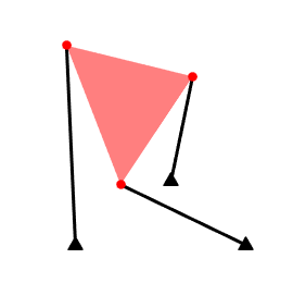
Figure 1: An example of a 3RPR mechanism.

A naive approach is to utilize a real monodromy group defined similarly as the (complex) monodromy group. This definition leads to heavy restrictions on the construction of real loops and can often cause no pertinent information to be gained in the computations as discussed in § 3.1. We instead propose a real monodromy structure to obtain piecewise information about the permutations of the real solutions outlined in § 3.2. In particular, this real monodromy structure contains all information regarding nonsingular assembly mode changes.

The remainder of the paper is as follows. Section 2 describes some background on the (complex) monodromy group. The real monodromy group and structure are described in Section 3 along with illustrative examples. Section 4 describes computing the real monodromy structure of a 3RPR mechanism where 2 of the legs can change length. Finally, the paper concludes in Section 5.

2 Monodromy group

Let $F(x;p)$ be a polynomial system with variables $x\in{\mathbb{C}}^{N}$ and parameters $p\in{\mathbb{C}}^{P}$. Assume that $F(x;p^{*})=0$ has $D\in{\mathbb{N}}$ isolated nonsingular solutions in ${\mathbb{C}}^{N}$ for generic $p^{*}\in{\mathbb{C}}^{P}$. That is, there is a Zariski open dense subset $U\subset{\mathbb{C}}^{P}$ such that $F(x;p^{*})=0$ has $D$ nonsingular isolated solutions in ${\mathbb{C}}^{N}$ for every $p^{*}\in U$. Fix a point $b\in U$ and let $x^{(1)},\dots,x^{(D)}\in{\mathbb{C}}^{N}$ be the $D$ nonsingular isolated solutions to $F(x;b)=0$. If ${\mathcal{S}}_{D}$ denotes the symmetric group on $D$ elements, then each loop $\gamma\subset U$ starting and ending at $b$ generates a permutation $\sigma_{\gamma}\in{\mathcal{S}}_{D}$ where $\sigma_{\gamma}(i)=j$ provided that the solution path of $F(x;p)=0$ over $\gamma$ starting at $x^{(i)}$ ends at $x^{(j)}$. The corresponding monodromy group is simply the collection of all such permutations, namely

$$\{\sigma_{\gamma}\in{\mathcal{S}}_{D}~{}|~{}\gamma\subset U\hbox{~{}is loop starting and ending at~{}}b\}.$$ (1)

The group structure arises naturally from concatenation of loops.

The monodromy group is independent of the choice $b\in U$ and the monodromy group of $F(x;p)$ for $p\in{\mathbb{C}}^{P}$ is equal to the monodromy group of $G(x;t)=F(x;\ell(t))$ where $\ell:{\mathbb{C}}\rightarrow{\mathbb{C}}^{P}$ is a general affine linear function [17]. In the one parameter case, the monodromy group is generated by the permutations arising from the finitely many loops that generate the fundamental group of the intersection of $U$ to the line parameterized by $\ell(t)$. This is described in detail with numerical algebraic geometric computations in [8] and illustrated in the following example.

Example 2.1

Consider the parameterized polynomial system

$$F(x;p)=\left[\begin{array}[]{c}x_{1}^{2}-x_{2}^{2}-p_{1}\\ 2x_{1}x_{2}-p_{2}\end{array}\right]=0$$

and $U=\{p\in{\mathbb{C}}^{2}~{}|~{}p_{1}^{2}+p_{2}^{2}\neq 0\}$. Thus, for every $p^{*}\in U$, $F(x;p^{*})=0$ has $D=4$ nonsingular isolated solutions in ${\mathbb{C}}^{2}$. We take $b=(1,0)\in U$ with corresponding solutions

$$x^{(1)}=(1,0),\hskip 14.22636ptx^{(2)}=(-1,0),\hskip 14.22636ptx^{(3)}=(0,\sqrt{-1}),\hskip 14.22636ptx^{(4)}=(0,-\sqrt{-1}).$$

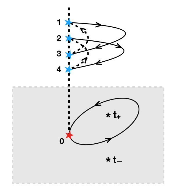
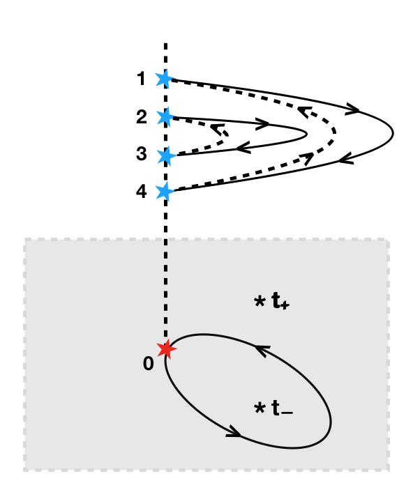
(a)	(b)

Figure 2: Illustration of (a) loop $\gamma_{+}$ and permutation $\sigma_{\gamma_{+}}$ and (b) loop $\gamma_{-}$ and permutation $\sigma_{\gamma_{-}}$

Consider restricting the parameter space to the line ${\mathcal{L}}\subset{\mathbb{C}}^{2}$ parameterized by $\ell(t)=(1-t,2t)$ so that $\ell(0)=b$. In particular, $U\cap{\mathcal{L}}\cong{\mathbb{C}}\setminus\{t_{+},t_{-}\}$ where $t_{\pm}=\frac{1\pm 2\sqrt{-1}}{5}$. Let $\gamma_{\pm}\subset{\mathbb{C}}$ be a simple loop starting and ending at $0$ which encircles $t_{\pm}$ but not $t_{\mp}$, respectively. The corresponding permutations, written in cycle notation, are

$$\sigma_{\gamma_{+}}=(1\hskip 4.2679pt3)(2\hskip 4.2679pt4)\hbox{~{}~{}~{}~{}~{}~{}and~{}~{}~{}~{}~{}~{}}\sigma_{\gamma_{-}}=(1\hskip 4.2679pt4)(2\hskip 4.2679pt3)$$

which are illustratively shown in Fig. 2. Therefore, the monodromy group is generated by the two permutations $\sigma_{\pm}$ which is the Klein group on four elements $K_{4}={\mathbb{Z}}_{2}\times{\mathbb{Z}}_{2}\subset{\mathcal{S}}_{4}$, namely

$$K_{4}=\{(1),\hskip 5.69054pt(1\hskip 4.2679pt2)(3\hskip 4.2679pt4),\hskip 5.69054pt(1\hskip 4.2679pt3)(2\hskip 4.2679pt4),\hskip 5.69054pt(1\hskip 4.2679pt4)(2\hskip 4.2679pt3)\}.$$ (2)

The reason for the defectivity of the monodromy group can be observed, for example, from the relation between $x_{1}$, $p_{1}$, and $p_{2}$, namely

$$4x_{1}^{4}-4x_{1}^{2}p_{1}-p_{2}^{2}=0$$

showing that the solutions arise in two pairs since

$$x_{1}=\pm\sqrt{\frac{p_{1}\pm\sqrt{p_{1}^{2}+p_{2}^{2}}}{2}}.$$

We note that if the monodromy group is the full symmetric group, computing corresponding permutations for a few random loops is generally sufficient to generate the full symmetric group [14]. Random monodormy loops can also be used effectively for performing numerical irreducible decomposition [2, 16].

3 Monodromy over the real numbers

Since many applications, particularly ones arising in science and engineering, are only interested in the real solutions, we consider monodromy action of real solutions over a real parameter space for a real polynomial system $F(x;p)$ where $x\in{\mathbb{R}}^{N}$ and $p\in{\mathbb{R}}^{P}$.

3.1 Real monodromy group

In the complex case, as summarized in § 2, loops arise on the nonempty Zariski open dense subset $U\subset{\mathbb{C}}^{P}$ consisting of parameter values where the number of nonsingular isolated complex solutions is constant. One can naively take a similar approach over the real numbers as follows. Fix a base point $b\in U\cap{\mathbb{R}}^{P}$ and let $R$ be the number of nonsingular isolated real solutions to $F(x;b)=0$. Hence, there is a connected open subset $U_{R}\subset{\mathbb{R}}^{P}$ containing $b$ such that the number of nonsingular isolated real solutions of $F(x;p^{*})=0$ is equal to $R$ for all $p^{*}\in U_{R}$. As in complex case, loops in $U_{R}$ yield permutations in ${\mathcal{S}}_{R}$. Following (1), the collection of all such permutations

$$\{\sigma_{\gamma}\in{\mathcal{S}}_{R}~{}|~{}\gamma\subset U_{R}\hbox{~{}is loop starting and ending at~{}}b\}$$ (3)

is the real monodromy group of $F(x;p)$ with base point $b$. This group is naturally independent of the choice of base point $b$ inside of $U_{R}$.

Example 3.1

Reconsider $F(x;p)$ from Ex. 2.1 with $b=(1,0)$. There are $R=2$ real solutions to $F(x;b)=0$, namely $x^{(1)}=(1,0)$ and $x^{(2)}=(-1,0)$. Since, for all $p^{*}\in U_{R}={\mathbb{R}}^{2}\setminus\{(0,0)\}$, $F(x;p^{*})=0$ has $2$ real solutions, the corresponding real monodromy group is generated by the loop $\gamma:[0,1]\rightarrow U_{R}$ where $\gamma(t)=(\cos(2\pi t),\sin(2\pi t))$ with $\gamma(0)=\gamma(1)=b$. This loops yields the permutation $\sigma_{\gamma}=(1\hskip 4.2679pt2)$ so that the corresponding real monodromy group is ${\mathcal{S}}_{2}=\{(1),(1\hskip 4.2679pt2)\}$.

In the complex case, there is a unique monodromy group based on the nonempty Zariski open dense subset $U\subset{\mathbb{C}}^{P}$. In the real case, there can be multiple real monodromy groups. The number of real solutions $R$ on the open set $U_{R}$ is called a typical number of nonsingular real solutions of $F(x;p)=0$. Thus, one has a real monodromy group of $F(x;p)$ for each typical number of nonsingular real solutions $R$ and each connected open subset $U_{R}$ in the set of all parameters $p^{*}\in{\mathbb{R}}^{P}$ for which $F(x;p^{*})=0$ has $R$ nonsingular isolated real solutions.

Example 3.2

The polynomial $F(x;p)=x^{2}+1-p^{2}$ has two typical number of real solutions, namely $0$ when $-1<p<1$ and $2$ when either $p<-1$ or $p>1$. The real monodromy group for $R=0$ and $U_{R}=(-1,1)\subset{\mathbb{R}}$ is empty since there are no real solutions. The real monodromy group for $R=2$ for both $U_{R}=(-\infty,-1)\subset{\mathbb{R}}$ and $U_{R}=(1,\infty)\subset{\mathbb{R}}$ is $\{(1)\}\subset{\mathcal{S}}_{2}$.

The previous illustrative examples suggest the following.

Theorem 3.3

Suppose that $F(x;p)$ is a real polynomial system with $x\in{\mathbb{R}}^{N}$ and $p\in{\mathbb{R}}^{P}$. Let $b\in{\mathbb{R}}^{P}$ such that $F(x;b)=0$ has $R>0$ nonsingular isolated real solutions and $U_{R}\subset{\mathbb{R}}^{P}$ which is a connected open set containing $b$ such that the number of nonsingular isolated real solutions of $F(x;p^{*})=0$ is equal to $R$ for all $p^{*}\in U_{R}$. If the fundamental group of $U_{R}$ is trivial, then the corresponding real monodromy group is $\{(1)\}\subset{\mathcal{S}}_{R}$. In particular, if $P=1$, then the corresponding real monodromy group is $\{(1)\}\subset{\mathcal{S}}_{R}$.

Proof.  If the fundamental group of $U_{R}$ is trivial, then all loops in $U_{R}$ are contractible yielding only the identity permutation in the real monodromy group. In particular, when $P=1$, then $U_{R}$ is an interval where all loops are contractible. $\Box$

The system from Ex. 3.1 was specifically designed to have a nontrivial real monodromy group. Since one often expects each corresponding set $U_{R}$ to be a cell thereby having a trivial fundamental group, one can often expect trivial real monodromy groups for problems arising in applications.

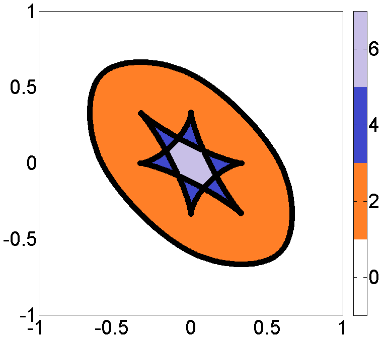
Figure 3: Parameter space ${\mathbb{R}}^{2}$ colored by number of nonsingular real solutions to (4).

Example 3.4

The Kuramoto model [13] provides a mathematical model of synchronous behavior of coupled oscillators. We consider $n=3$ oscillators and avoid the trivial rotation by fixing $\theta_{3}=0$. For parameters $\omega=(\omega_{1},\omega_{2})$, the steady-state solutions of the Kuramoto model satisfy

$$\left[\begin{array}[]{c}\sin(\theta_{1}-\theta_{2})+\sin(\theta_{1}-\theta_{3})-3\omega_{1}\\ \sin(\theta_{2}-\theta_{1})+\sin(\theta_{2}-\theta_{3})-3\omega_{2}\end{array}\right]=0.$$

We convert to a polynomial system by taking $s_{i}=\sin(\theta_{i})$ and $c_{i}=\cos(\theta_{i})$, namely

$$F(s_{1},c_{1},s_{2},c_{2};\omega_{1},\omega_{2})=\left[\begin{array}[]{c}(s_{1}c_{2}-c_{1}s_{2})+(s_{1}c_{3}-c_{1}s_{3})-3\omega_{1}\\ (s_{2}c_{1}-c_{2}s_{1})+(s_{2}c_{3}-c_{2}s_{3})-3\omega_{2}\\ s_{1}^{2}+c_{1}^{2}-1\\ s_{2}^{2}+c_{2}^{2}-1\\ \end{array}\right].$$ (4)

Figure 3 adapted from [4, Fig. 2] colors the parameters based on the number of real solutions. In particular, the connected set having $6$ real solutions and each of the six connected sets having $4$ real solutions have trivial fundamental group and thus trivial real monodromy group. The connected set having $2$ real solutions has a nontrivial fundamental group, but one can check that this set also has a trivial real monodromy group. The reason for this will become apparent in Ex. 3.15. Moreover, the (complex) monodromy group computed using [8] is ${\mathcal{S}}_{6}$, which is not a solvable group.

The condition that the number of nonsingular real solutions along loops in the real parameter space remain constant is a restriction that both ensures a group structure and is responsible for often having a trivial real monodromy group. The following provides an illustration of this restriction.

Example 3.5

Consider the parameterized polynomial system

$$F(x;p)=\left[\begin{array}[]{c}(x_{1}^{2}-x_{2}^{2}-p_{1})(x_{1}^{2}+p_{1})\\ 2x_{1}x_{2}-p_{2}\end{array}\right]=0$$ (5)

which is a modification of the system considered in Ex. 2.1 and 3.1. For $b=(-1,0)$, there are $R=4$ nonsingular real solutions, namely:

$$x^{(1)}=(1,0),\hskip 14.22636ptx^{(2)}=(-1,0),\hskip 14.22636ptx^{(3)}=(0,1),\hskip 14.22636ptx^{(4)}=(0,-1).$$

In this case, $U_{R}=\{p_{1}<0\}\subset{\mathbb{R}}^{2}$ which has a trivial fundamental group and thus the real monodromy group is trivial. Figure 4 illustrates the decomposition of the parameter space based on the number of real solutions.

Consider the loop $\gamma(t)=(-\cos(2\pi t),\sin(2\pi t))$ for $t\in[0,1]$ starting and ending at $b$. If we only focus on the two solution paths starting at $x^{(1)}$ and $x^{(2)}$, these paths remain nonsingular over the loop and the endpoints interchange as one would expect from the real monodromy group in Ex. 3.1. The two solution paths starting at $x^{(3)}$ and $x^{(4)}$ are nonsingular and real for $t\in[0,1/4)\cup(3/4,1]$, nonsingular and nonreal for $t\in(1/4,3/4)$, and at infinity for $t\in\{1/4,3/4\}$.

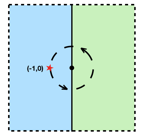
Figure 4: Parameter space ${\mathbb{R}}^{2}$, colored by number of nonsingular real solutions for $F(x;p)$ in (5): $2$ on $\{p_{1}>0\}$ (green) and $4$ on $\{p_{1}<0\}$ (blue), base point $b=(-1,0)$, and loop $\gamma(t)$.

Example 3.4 shows that important information about the connections between some of the real solutions can be obtained by relaxing the requirement that all real solutions remain nonsingular along the path. With this relaxation, one may lose the group structure, but obtains a complete picture of the interconnections between the real solutions over a base point $b$, which is described next.

3.2 Real monodromy structure

Writing the monodromy action as a group of permutations provides an efficient representation of the behavior of the solutions. When the action under consideration may no longer be a group, we propose a structure to encode the action called the real monodromy structure.

The following summarizes some sets of interest.

Definition 3.6

For a nonnegative integer $R$, let $\operatorname*{{\rm Pow}}(R)$ be the power set of $\{1,\dots,R\}$ which is the set of all subsets of $\{1,\dots,R\}$. Let $\operatorname*{{\rm OPow}}(R)$ be the ordered power set of $\{1,\dots,R\}$ which is the set of all ordered subsets of $\{1,\dots,R\}$. For $0\leq k\leq R$, let $\operatorname*{{\rm OPow}}_{k}(R)$ be the $k$-ordered power set of $\{1,\dots,R\}$ which is the set of all ordered subsets of $\{1,\dots,R\}$ of size $k$. Let $\operatorname*{{\rm IPow}}_{k}(R)$ be the subset of $\operatorname*{{\rm OPow}}_{k}(R)$ where the entries of the elements are listed in increasing order.

Example 3.7

To illustrate, we consider $R=2$. Thus,

• $\operatorname*{{\rm Pow}}(2)=\{\emptyset,\{1\},\{2\},\{1,2\}\}$   and    $\operatorname*{{\rm OPow}}(2)=\{\emptyset,\{1\},\{2\},\{1,2\},\{2,1\}\}$;

• $\operatorname*{{\rm OPow}}_{0}(2)=\{\emptyset\}$;

• $\operatorname*{{\rm OPow}}_{1}(2)=\{\{1\},\{2\}\}=\operatorname*{{\rm IPow}}_{1}(2)$;

• $\operatorname*{{\rm OPow}}_{2}(2)=\{\{1,2\},\{2,1\}\}$   and    $\operatorname*{{\rm IPow}}_{2}(2)=\{\{1,2\}\}$.

In particular, for elements in the power set, order does not matter. Order does matter for elements in the ordered power set.

With this notation, we present the real monodromy structure.

Definition 3.8

For the real parameterized polynomial system $F(x;p)$, fix a base point $b\in{\mathbb{R}}^{P}$ and let $x^{(1)},\dots,x^{(R)}\in{\mathbb{R}}^{N}$ be the $R$ nonsingular isolated solutions of $F(x;b)=0$. The real monodromy structure of $F$ at $b$ is a collection ${\mathcal{G}}_{\bullet}=\{{\mathcal{G}}_{1},\dots,{\mathcal{G}}_{R}\}$ of functions

$${\mathcal{G}}_{k}:{\operatorname*{{\rm IPow}}}_{k}(R)\rightarrow\operatorname*{{\rm Pow}}({\operatorname*{{\rm OPow}}}_{k}(R))$$

for $k=1,\dots,R$ constructed as follows. For each $\mathcal{Q}=\{q_{1},...,q_{k}\}\in\operatorname*{{\rm IPow}}_{k}(R)$, ${\mathcal{G}}_{k}(\mathcal{Q})$ is the collection of subsets of $\operatorname*{{\rm OPow}}_{k}(R)$ of the form $\{s_{1},...,s_{k}\}\in\operatorname*{{\rm OPow}}_{k}(R)$ such that there exists a loop $\gamma\subset{\mathbb{R}}^{P}$ starting and ending at $b$ where the solution path of $F(x;p)=0$ over $\gamma$ starting at $x^{(q_{i})}$ is nonsingular and ends at $x^{(s_{i})}$ for $i=1,\dots,k$.

The real monodromy group describes how the set of all solutions can be permuted whereas the real monodromy structure describes how each subset of solutions can be permuted. Hence, the real monodromy group is encoded in ${\mathcal{G}}_{R}$.

Example 3.9

Consider representing the real monodromy group ${\mathcal{S}}_{2}$ from Ex. 3.1 as a real monodromy structure. First, we construct the map ${\mathcal{G}}_{1}$. Since both corresponding solutions can trivially return to themselves or connect to the other, ${\mathcal{G}}_{1}$ maps both $\{1\}$ and $\{2\}$ to $\{\{1\},\{2\}\}$. Similarly, ${\mathcal{G}}_{2}$ maps $\{1,2\}$ to $\{\{1,2\},\{2,1\}\}$ since the pair can remain unchanged or be permuted. For simplicity, we will write ${\mathcal{G}}_{\bullet}=\{{\mathcal{G}}_{1},{\mathcal{G}}_{2}\}$ as

• $\mathcal{G}_{1}$

  • $\{1\},\{2\}\mathrel{\ooalign{$\rightarrow$\cr\kern-0.6458pt\raise 1.18399pt\hbox{\scalebox{1.0}[0.522]{$\mid$}}\cr}}\{\{1\},\{2\}\}$

• $\mathcal{G}_{2}$

  • $\{1,2\}\mathrel{\ooalign{$\rightarrow$\cr\kern-0.6458pt\raise 1.18399pt\hbox{\scalebox{1.0}[0.522]{$\mid$}}\cr}}\{\{1,2\},\{2,1\}\}$.

Example 3.10

For Ex. 3.5 with $b=(-1,0)$, the real monodromy structure is ${\mathcal{G}}_{\bullet}=\{{\mathcal{G}}_{1},\dots,{\mathcal{G}}_{4}\}$:

• $\mathcal{G}_{1}$

  • $\{1\},\{2\}\mathrel{\ooalign{$\rightarrow$\cr\kern-0.6458pt\raise 1.18399pt\hbox{\scalebox{1.0}[0.522]{$\mid$}}\cr}}\{\{1\},\{2\}\}$

  • $\{q_{1}\}\mathrel{\ooalign{$\rightarrow$\cr\kern-0.6458pt\raise 1.18399pt\hbox{\scalebox{1.0}[0.522]{$\mid$}}\cr}}\{\{q_{1}\}\}$ for all others

• $\mathcal{G}_{2}$

  • $\{1,2\}\mathrel{\ooalign{$\rightarrow$\cr\kern-0.6458pt\raise 1.18399pt\hbox{\scalebox{1.0}[0.522]{$\mid$}}\cr}}\{\{1,2\},\{2,1\}\}$

  • $\{q_{1},q_{2}\}\mathrel{\ooalign{$\rightarrow$\cr\kern-0.6458pt\raise 1.18399pt\hbox{\scalebox{1.0}[0.522]{$\mid$}}\cr}}\{\{q_{1},q_{2}\}\}$ for all others

• $\mathcal{G}_{3}$

  • $\{q_{1},q_{2},q_{3}\}\mathrel{\ooalign{$\rightarrow$\cr\kern-0.6458pt\raise 1.18399pt\hbox{\scalebox{1.0}[0.522]{$\mid$}}\cr}}\{\{q_{1},q_{2},q_{3}\}\}$

• $\mathcal{G}_{4}$

  • $\{q_{1},q_{2},q_{3},q_{4}\}\mathrel{\ooalign{$\rightarrow$\cr\kern-0.6458pt\raise 1.18399pt\hbox{\scalebox{1.0}[0.522]{$\mid$}}\cr}}\{\{q_{1},q_{2},q_{3},q_{4}\}\}$.

This shows that there is an interconnection between $x^{(1)}$ and $x^{(2)}$ as described by the loop $\gamma(t)$ in Ex. 3.5, whereas anything involving $x^{(3)}$ or $x^{(4)}$ must be trivial. The function ${\mathcal{G}}_{4}$ encodes the triviality of the real monodromy group. Moreover, ${\mathcal{G}}_{\bullet}$ does not have a group structure since ${\mathcal{G}}_{4}$ is trivial while ${\mathcal{G}}_{1}$ and ${\mathcal{G}}_{2}$ are not.

Remark 3.11

A nonsingular assembly mode change means that there is a real nonsingular path between solution $x^{(i)}$ and $x^{(j)}$ where $i\neq j$. Hence, nonsingular assembly mode changes are described by ${\mathcal{G}}_{1}$, namely $i\neq j$ such that $\{j\}\in{\mathcal{G}}_{1}(\{i\})$.

A group $G\subset{\mathcal{S}}_{R}$ is said to be $k$-transitive if, for every $\mathcal{Q}=\{q_{1},...,q_{k}\}\in\operatorname*{{\rm IPow}}_{k}(R)$ and $\mathcal{T}=\{t_{1},...,t_{k}\}\in\operatorname*{{\rm OPow}}_{k}(R)$, there exists $\sigma\in G$ such that $\sigma(q_{i})=t_{i}$ for $i=1,\dots,k$. Clearly, if $G$ is $k$-transitive for $k>1$, then $G$ is also $(k-1)$-transitive. If $G$ is $1$-transitive, then $G$ is called transitive.

Example 3.12

The group $K_{4}\subset{\mathcal{S}}_{4}$ in (2) is transitive. It is not $2$-transitive since there does not exist $\sigma\in K_{4}$ which maps the ordered set $\{1,2\}$ to the ordered set $\{1,3\}$.

The following extends the notion of transitivity to the real monodromy structure.

Definition 3.13

A real monodromy structure ${\mathcal{G}}_{\bullet}=\{{\mathcal{G}}_{1},\dots,{\mathcal{G}}_{R}\}$ is $k$-transitive if

$${\mathcal{G}}_{k}(\mathcal{Q})={\operatorname*{{\rm OPow}}}_{k}(R)\in\operatorname*{{\rm Pow}}({\operatorname*{{\rm OPow}}}_{k}(R))$$

for every $\mathcal{Q}\in\operatorname*{{\rm IPow}}_{k}(R)$.

Clearly, if ${\mathcal{G}}_{\bullet}$ is $k$-transitive for $k>1$, then ${\mathcal{G}}_{\bullet}$ is also $(k-1)$-transitive. Moreover, ${\mathcal{G}}_{\bullet}$ is called transitive if it is $1$-transitive. Hence, a real monodromy structure is transitive if and only if ${\mathcal{G}}_{1}(\{i\})=\{\{1\},\dots,\{R\}\}=\operatorname*{{\rm OPow}}_{1}(R)$ for all $i=1,\dots,R$ meaning that, for every $i,j\in\{1,\dots,R\}$, there is a nonsingular solution path starting at $x^{(i)}$ and ending at $x^{(j)}$.

Example 3.14

The real monodromy structure ${\mathcal{G}}_{\bullet}$ in Ex. 3.9 is $2$-transitive and hence $1$-transitive. The real monodromy stucture ${\mathcal{G}}_{\bullet}$ in Ex. 3.10 is not transitive.

We conclude this section with an illustrative description of computing the real monodromy structure for the Kuramoto model in (4) which is dependent on 2 parameters.

Example 3.15

For the $n=3$ Kuramoto system $F$ in (4), Ex. 3.4 showed that every real monodromy group is trivial and the (complex) monodromy group is the full symmetric group ${\mathcal{S}}_{6}$. The following computes the real monodromy structure ${\mathcal{G}}_{\bullet}$ at $\omega^{*}=(0,0)$, which is nontrivial thereby identifying interconnections between the real solutions. At $\omega^{*}$, we label the six solutions as

$$\begin{array}[]{c}x^{(1)}=(0,1,0,1),\hskip 14.22636ptx^{(2)}=(0,1,0,-1),\hskip 14.22636ptx^{(3)}=(0,-1,0,1),\hskip 14.22636ptx^{(4)}=(0,-1,0,-1),\\[3.61371pt] x^{(5)}=\frac{1}{2}(\sqrt{3},-1,-\sqrt{3},-1),\hskip 14.22636ptx^{(6)}=\frac{1}{2}(-\sqrt{3},-1,\sqrt{3},-1).\end{array}$$

First, one decomposes the parameter space into connected components based on the number of real solutions. Figure 3 was generated, for example, using [6] via Bertini [1]. Since the connected hexagonal region containing $\omega^{*}$ has a trivial fundamental group, it follows that both ${\mathcal{G}}_{5}$ and ${\mathcal{G}}_{6}$ are trivial. Moreover, since the curved “hexagram,” i.e., “six-sided star,” region consisting of the set of parameter values with at least $4$ real solutions also has a trivial fundamental group, ${\mathcal{G}}_{3}$ and ${\mathcal{G}}_{4}$ must also be trivial. Hence, we only need to consider ${\mathcal{G}}_{1}$ and ${\mathcal{G}}_{2}$.

To help with the bookkeeping, we fix a marked point in each connected component with $\omega^{*}$ being the one in its component and place an ordering on the real solutions over each marked point. Then, in the two parameter case, we identify each of the finitely many smooth segments of the boundaries of the connected components. Along such segments of the boundary, there is a consistent identification of the real solutions which are no longer nonsingular at the boundary. Thus, there is an equivalence along each smooth segment of the boundary. A similar statement holds for smooth regions of the boundary when there are more parameters.

From Fig. 3, there are $18$ smooth boundary segments to consider: $6$ for the region having $6$ real solutions and two additional ones for each of the $6$ regions having $4$ real solutions. A homotopy is used to identify the behavior of the solutions between each boundary segment using the consistent ordering from the marked point of the region. Intermediate points can be used to assist in this, which are especially useful in nonconvex regions to connect the marked points as shown in Fig. 5.

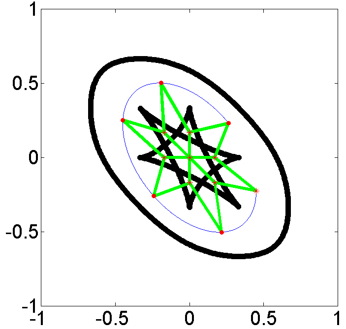
Figure 5: A plot of the boundaries of the connected components (black lines) for (4), selected marked points (red star) in each connected component, all intermediary points (red dot), paths crossing the boundary (green lines), and connections between intermediate points and the marked point of the component (blue curves).

Finally, an analysis of the data generated from traversing the boundaries produces all of the possible interconnections between the real solutions $x^{(1)},\dots,x^{(6)}$ at $\omega^{*}$. In particular, this analysis shows that the hexagram region consists of two large curved triangles: one pointing northwest and the other point southeast. On the boundary of the northwest triangle, $x^{(6)}$ always becomes singular and merges with one of $x^{(2)}$, $x^{(3)}$, or $x^{(4)}$ along its three sides. Similarly, for the boundary of the southeast triangle, $x^{(5)}$ always becomes singular and merges with one of $x^{(2)}$, $x^{(3)}$, or $x^{(4)}$ along its three sides. Since one must cross both triangular boundaries, to possibly have a nontrivial action, we know that ${\mathcal{G}}_{1}$ and ${\mathcal{G}}_{2}$ applied to any set involving either $5$ or $6$ is trivial.

Furthermore, this analysis shows that the solution sheet corresponding to $x^{(1)}$ over the colored region of the parameter space in Fig. 3 is nonsingular. In particular, this explains why the real monodromy group computed in Ex. 3.4 for the connected component colored orange in Fig. 3 having 2 real solutions is trivial even though the fundamental group for this component is not trivial. Hence, ${\mathcal{G}}_{1}(\{1\})=\{\{1\}\}$ but it is different than $x^{(5)}$ and $x^{(6)}$ in that it can be included in nontrivial ${\mathcal{G}}_{2}$ action. In fact, since it is possible to move from $\omega^{*}$ into this orange component using nonsingular paths starting at $x^{(1)}$ and one of $x^{(2)}$, $x^{(3)}$, or $x^{(4)}$, we have that ${\mathcal{G}}_{1}$ is transitive on $\{2\}$, $\{3\}$, and $\{4\}$ and ${\mathcal{G}}_{2}$ is transitive on $\{1,2\}$, $\{1,3\}$, and $\{1,4\}$. This is summarized in the following:

• $\mathcal{G}_{1}$

  • $\{2\},\{3\},\{4\}\mathrel{\ooalign{$\rightarrow$\cr\kern-0.6458pt\raise 1.18399pt\hbox{\scalebox{1.0}[0.522]{$\mid$}}\cr}}\{\{2\},\{3\},\{4\}\}$

  • $\{q_{1}\}\mathrel{\ooalign{$\rightarrow$\cr\kern-0.6458pt\raise 1.18399pt\hbox{\scalebox{1.0}[0.522]{$\mid$}}\cr}}\{\{q_{1}\}\}$ for all others

• $\mathcal{G}_{2}$

  • $\{1,2\},\{1,3\},\{1,4\}\mathrel{\ooalign{$\rightarrow$\cr\kern-0.6458pt\raise 1.18399pt\hbox{\scalebox{1.0}[0.522]{$\mid$}}\cr}}\{\{1,2\},\{1,3\},\{1,4\}\}$

  • $\{q_{1},q_{2}\}\mathrel{\ooalign{$\rightarrow$\cr\kern-0.6458pt\raise 1.18399pt\hbox{\scalebox{1.0}[0.522]{$\mid$}}\cr}}\{\{q_{1},q_{2}\}\}$ for all others.

Therefore, the real monodromy structure provides three distinct groups of solutions which have similar properties: $\{x^{(1)}\}$, $\{x^{(2)},x^{(3)},x^{(4)}\}$, and $\{x^{(5)},x^{(6)}\}$.

4 Real monodromy of the 3RPR mechanism

The 3RPR mechanism, as shown in Fig. 1, is a well-known mechanism that has a nonsingular assembly mode change [5, 9, 18, 12, 15, 3, 11]. Thus, with an appropriate choice of base point, ${\mathcal{G}}_{1}$ of the real monodromy structure for this base point will be nontrivial. In this section, we compute the complete real monodromy structure ${\mathcal{G}}_{\bullet}$ using a base point from [11] when one of the leg lengths is fixed and the other two legs are free to change lengths.

As shown in Fig. 6, let the leg lengths be $\ell_{1}$, $\ell_{2}$, and $\ell_{3}$. For simplicity, we will consider the squares of the leg lengths, namely $c_{i}=\ell_{i}^{2}$. In the fixed frame, set the three anchors of the three legs, respectively, at $(0,0)$, $(A_{2},0)$, and $(A_{3},B_{3})$. In the moving frame, set the three connections of the three legs, respectively, attached to the triangle at $P_{1}=(0,0)$, $P_{2}=(a_{2},0)$, and $P_{3}=(a_{3},b_{3})$. Following the case studied in [11], we take the following constants:

$$a_{2}=14,\hskip 5.69054pta_{3}=7,\hskip 5.69054ptb_{3}=10,\hskip 5.69054ptA_{2}=16,\hskip 5.69054ptA_{3}=9,\hskip 5.69054ptB_{3}=6,\hskip 5.69054ptc_{3}=\ell_{3}^{2}=100.$$ (6)

For the parameters $c=(c_{1},c_{2})$, we take the base point, corresponding to the “home” position, to be $c^{*}=(75,70)$ as in [11] where the mechanisms satisfying this setup are shown in Fig. 7.

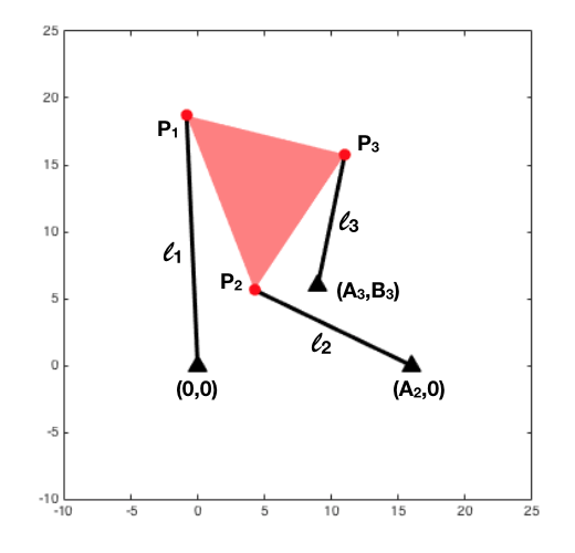
Figure 6: An illustration of a 3RPR mechanism.

The variables $(p,\phi)=(p_{1},p_{2},\phi_{1},\phi_{2})$ of the polynomial system represent the relative position and rotation between fixed frame and moving frame, respectively. The polynomials constrain the rotation $(\phi_{1},\phi_{2})$ to a point on the unit circle and describe the three leg constraints:

$$F(p,\phi;c)=\left[\begin{array}[]{l}\phi_{1}^{2}+\phi_{2}^{2}-1\\ p_{1}^{2}+p_{2}^{2}-2(a_{3}p_{1}+b_{3}p_{2})\phi_{1}+2(b_{3}p_{1}-a_{3}p_{2})\phi_{2}+a_{3}^{2}+b_{3}^{2}-c_{1}\\ p_{1}^{2}+p_{2}^{2}-2A_{2}p_{1}+2((a_{2}-a_{3})p_{1}-b_{3}p_{2}+A_{2}a_{3}-A_{2}a_{2})\phi_{1}\\ \hskip 28.45274pt+~{}2(b_{3}p_{1}+(a_{2}-a_{3})p_{2}-A_{2}b_{3})\phi_{2}+(a_{2}-a_{3})^{2}+b_{3}^{2}+A_{2}^{2}-c_{2}\\ p_{1}^{2}+p_{2}^{2}-2(A_{3}p_{1}+B_{3}p_{2})+A_{3}^{2}+B_{3}^{2}-c_{3}\end{array}\right].$$

At the “home” position $c^{*}=(75,70)$, the system $F(p,\phi;c^{*})=0$ has $6$ nonsingular real solutions which are assigned labels $x^{(1)},\dots,x^{(6)}$ in Fig. 7. The remaining part of this section describes computing the real monodromy structure ${\mathcal{G}}_{\bullet}=\{{\mathcal{G}}_{1},\dots,{\mathcal{G}}_{6}\}$ for $F$ at $c^{*}$ where we utilize Bertini [1] to perform the homotopy continuation computations.

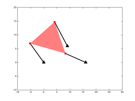
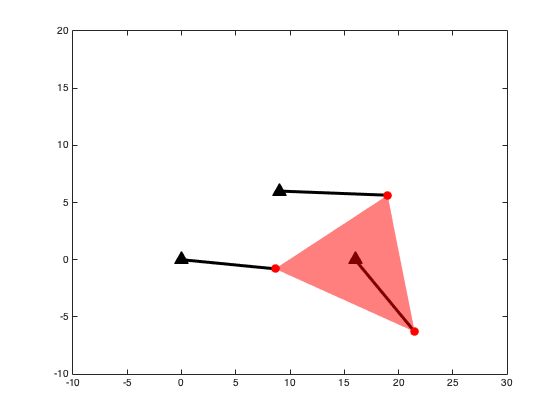
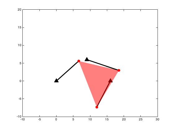
$x^{(1)}$	$x^{(2)}$	$x^{(3)}$
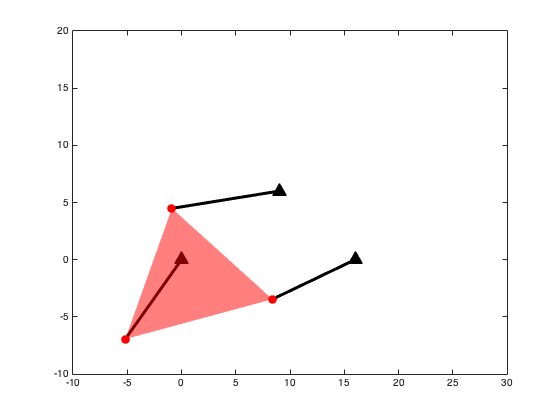
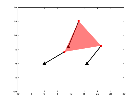
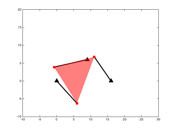
$x^{(4)}$	$x^{(5)}$	$x^{(6)}$

Figure 7: The $6$ solutions to $F(p,\phi;c^{*})=0$.

First, we compute the boundaries of the subsets of ${\mathbb{R}}^{2}$ where the number of real solutions change using [6]. Figure 8 colors the regions in $c=(c_{1},c_{2})\in{\mathbb{R}}^{2}$ having $0$, $2$, $4$, and $6$ real solutions, where $c^{*}=(75,70)$ lies in the unique connected component having $6$ real solutions. In particular, since this component has a trivial fundamental group, Theorem 3.3 concludes that the real monodromy group is trivial. It follows that ${\mathcal{G}}_{5}$ and ${\mathcal{G}}_{6}$ are also trivial. We note that the (complex) monodromy group is ${\mathcal{S}}_{6}$ showing there is no complex structure in the solutions encoded by the monodromy group.

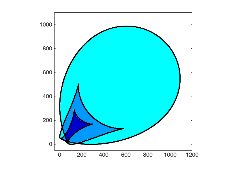
(a)

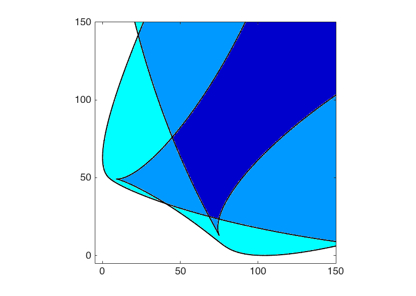
(b)

Figure 8: Regions of the parameter space $c=(c_{1},c_{2})$ colored by the number of real solutions where (a) is the full view and (b) is a zoomed in view of the lower left corner. The navy blue region has 6 real solutions, the grey blue region has 4 real solutions, the baby blue region has 2 real solutions, and the white region has 0 real solutions.

To help with the bookkeeping, we fix a marked point in each connected component and select additional intermediate points to simplify the computation of loops as shown in Fig. 9. To compute all possible loops, we need to transverse between the connected components. Since there is an equivalence by passing through smooth regions of the boundary, there are only finitely many possible loops of interest. For example, leaving the navy blue region having 6 real solutions and entering into the largest grey blue connected component that touches it has at most three different outcomes obtained by crossing through the three different smooth segments of the boundary. The intermediate points facilitate moving the solutions to the marked point to have consistent ordering.

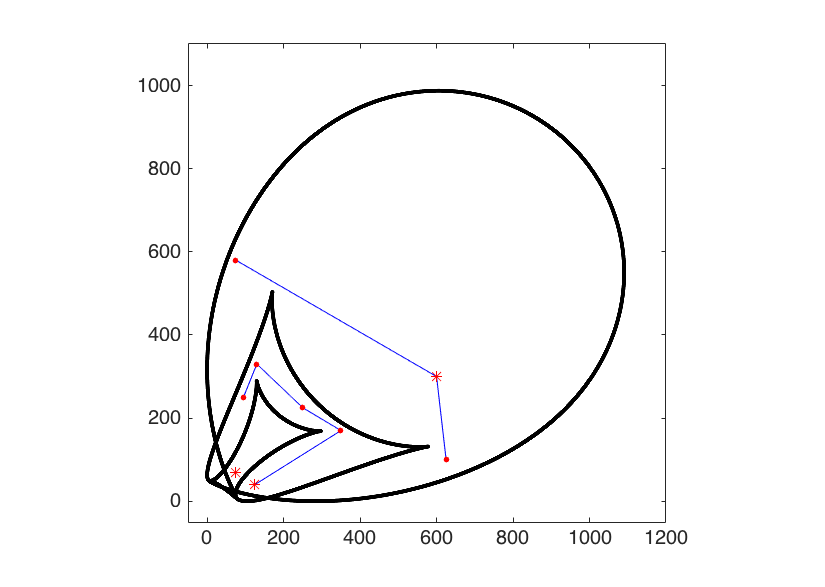
(a)

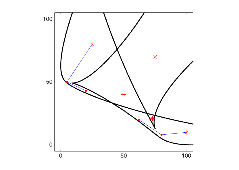
(b)

Figure 9: Selected marked points (red star) in each connected component and all intermediary points (red dot) in (a) full view and (b) zoomed in view of the lower left corner.

By tracking solutions along all possible loops and carefully keeping track of those that remain nonsingular, we obtain the following real monodromy structure where ${\mathcal{G}}_{5}$ and ${\mathcal{G}}_{6}$ are trivial:

• $\mathcal{G}_{1}$

  • $\{1\},\{2\},\{3\}\mathrel{\ooalign{$\rightarrow$\cr\kern-0.6458pt\raise 1.18399pt\hbox{\scalebox{1.0}[0.522]{$\mid$}}\cr}}\{\{1\},\{2\},\{3\}\}$

  • $\{4\},\{5\},\{6\}\mathrel{\ooalign{$\rightarrow$\cr\kern-0.6458pt\raise 1.18399pt\hbox{\scalebox{1.0}[0.522]{$\mid$}}\cr}}\{\{4\},\{5\},\{6\}\}$

• $\mathcal{G}_{2}$

  • $\{1,4\},\{1,5\},\{1,6\},\{2,5\},\{2,6\},\{3,4\},\{3,5\}\mathrel{\ooalign{$\rightarrow$\cr\kern-0.6458pt\raise 1.18399pt\hbox{\scalebox{1.0}[0.522]{$\mid$}}\cr}}\left\{\begin{array}[]{c}\{1,4\},\{1,5\},\{1,6\},\{2,5\},\\ \{2,6\},\{3,4\},\{3,5\}\end{array}\right\}$

  • $\{1,3\},\{2,3\}\mathrel{\ooalign{$\rightarrow$\cr\kern-0.6458pt\raise 1.18399pt\hbox{\scalebox{1.0}[0.522]{$\mid$}}\cr}}\{\{1,3\},\{2,3\}\}$

  • $\{4,6\},\{5,6\}\mathrel{\ooalign{$\rightarrow$\cr\kern-0.6458pt\raise 1.18399pt\hbox{\scalebox{1.0}[0.522]{$\mid$}}\cr}}\{\{4,6\},\{5,6\}\}$

  • $\{q_{1},q_{2}\}\mathrel{\ooalign{$\rightarrow$\cr\kern-0.6458pt\raise 1.18399pt\hbox{\scalebox{1.0}[0.522]{$\mid$}}\cr}}\{\{q_{1},q_{2}\}\}$ for all others

• $\mathcal{G}_{3}$

  • $\{1,4,6\},\{1,5,6\},\{2,5,6\}\mathrel{\ooalign{$\rightarrow$\cr\kern-0.6458pt\raise 1.18399pt\hbox{\scalebox{1.0}[0.522]{$\mid$}}\cr}}\{\{1,4,6\},\{1,5,6\},\{2,5,6\}\}$

  • $\{1,3,6\},\{2,3,6\}\mathrel{\ooalign{$\rightarrow$\cr\kern-0.6458pt\raise 1.18399pt\hbox{\scalebox{1.0}[0.522]{$\mid$}}\cr}}\{\{1,3,6\},\{2,3,6\}\}$

  • $\{3,4,6\},\{3,5,6\}\mathrel{\ooalign{$\rightarrow$\cr\kern-0.6458pt\raise 1.18399pt\hbox{\scalebox{1.0}[0.522]{$\mid$}}\cr}}\{\{3,4,6\},\{3,5,6\}\}$

  • $\{q_{1},q_{2},q_{3}\}\mathrel{\ooalign{$\rightarrow$\cr\kern-0.6458pt\raise 1.18399pt\hbox{\scalebox{1.0}[0.522]{$\mid$}}\cr}}\{\{q_{1},q_{2},q_{3}\}\}$ for all others

• $\mathcal{G}_{4}$

  • $\{1,3,4,6\},\{1,3,5,6\},\{2,3,5,6\}\mathrel{\ooalign{$\rightarrow$\cr\kern-0.6458pt\raise 1.18399pt\hbox{\scalebox{1.0}[0.522]{$\mid$}}\cr}}\{\{1,3,4,6\},\{1,3,5,6\},\{2,3,5,6\}\}$

  • $\{q_{1},q_{2},q_{3},q_{4}\}\mathrel{\ooalign{$\rightarrow$\cr\kern-0.6458pt\raise 1.18399pt\hbox{\scalebox{1.0}[0.522]{$\mid$}}\cr}}\{\{q_{1},q_{2},q_{3},q_{4}\}\}$ for all others

Figures 10 and 11 illustrate a nonsingular assembly mode change between $x^{(4)}$ and $x^{(5)}$.

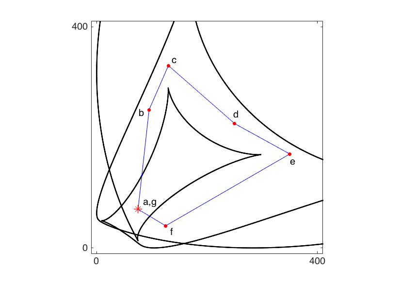
Figure 10: A loop starting and ending at $c^{*}=(75,70)$ that yields a nonsingular assembly mode change. The corresponding linkage pose for the labeled points are shown in Fig. 11.

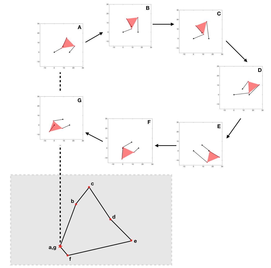
Figure 11: Solutions along a loop that yields a nonsingular assembly mode change.

The real monodromy structure ${\mathcal{G}}_{\bullet}$ identifies that the real solutions arise in two groups of three solutions coinciding with the results in [11] which showed that there are two disjoint path-connected components. In fact, in light of this constraint, ${\mathcal{G}}_{1}$ shows that all possible nonsingular assembly mode changes can occur. The real monodromy structure ${\mathcal{G}}_{\bullet}$ provides additional information beyond nonsingular assembly mode changes by considering how other subsets of solutions can be interchanged. For example, ${\mathcal{G}}_{4}$ shows that it is possible to interchange two solutions $x^{(1)}$ and $x^{(2)}$ while having three solutions $x^{(3)}$, $x^{(5)}$, and $x^{(6)}$ return to themselves with all four paths remaining real and nonsingular. It is also possible to interchange two pairs of solutions $x^{(1)}$ and $x^{(2)}$, and $x^{(4)}$ and $x^{(5)}$ while having two solutions $x^{(3)}$ and $x^{(6)}$ return to themselves with all four paths remaining real and nonsingular.

5 Conclusion

The (complex) monodromy group is a classically used invariant in algebraic geometry to study the structure of solutions to a parameterized system of polynomial equations. Since many applications involve working with real solution sets over real parameter spaces, an extension of the monodromy action computations to the real numbers is needed. A naive extension is to consider loops where all real solutions stay real and nonsingular along the solution path yielding the real monodromy group. However, this is very restrictive and is often trivial. Thus, we propose a real monodromy structure that gives tiered information on the monodromy actions for the real solutions. This enables useful structural information to be obtained and circumvents the restrictiveness of the naive extension by relaxing the condition that all real paths remain nonsingular.

The real monodromy structure for the 3RPR mechanism allowing two legs to change length describes how the solutions can interchange thereby providing a complete mathematical generalization of nonsingular assembly mode changes. This information can be useful, for example, in calibration. If no real solutions can interchange, i.e., the real monodromy structure is trivial, then returning to the “home” position avoiding singularities will always yield the same pose. However, if the real monodromy structure is not trivial, then it describes all possible interconnections between poses over the “home” position. Future work includes computing real monodromy structures for Stewart-Gough platforms.

6 Acknowledgments

The authors thank Charles Wampler for helpful discussions on kinematics and 3RPR mechanism.

References

- [1] D.J. Bates, J.D. Hauenstein, A.J. Sommese, and C.W. Wampler, Bertini: Software for numerical algebraic geometry. Available at bertini.nd.edu.
- [2] D.J. Bates, J.D. Hauenstein, A.J. Sommese, and C.W. Wampler, Numerically Solving Polynomial Systems with Bertini. SIAM, Philadelphia, 2013.
- [3] I. Bonev, S. Briot, P. Wenger, and D. Chablat, Changing assembly modes without passing parallel singularities in non-cuspidal parallel robots. In Proceedings of the Second Int. Workshop on Fundamental Issues and Future Research Directions for Parallel Mechanisms and Manipulators, 2008, pp. 197–200.
- [4] O. Coss, J.D. Hauenstein, H. Hong, and D.K. Molzahn, Locating and counting equilibria of the Kuramoto model with rank one coupling. SIAM J. Appl. Alg. Geom., 2(1):45–71, 2018.
- [5] C.M. Gosselin, J. Sefrioui, and M.J. Richards, Solutions Polynomiales au Problème de la Cinématique Directe des Manipulateurs Parallèles Plans à Trois Degrés de Liberté. Mehc. Mach. Theory, 27(2):1007–1019, 1992.
- [6] H.A. Harrington, D. Mehta, H.M. Byrne, and J.D. Hauenstein, Decomposing the parameter space of biological networks via a numerical discriminant approach. Preprint available at www.nd.edu/~jhauenst/preprints/hmbhCellNetwork.pdf.
- [7] J. Harris, Galois groups of enumerative problems. Duke Math. J., 46:685–724, 1979.
- [8] J.D. Hauenstein, J.I. Rodriguez, and F. Sottile, Numerical computation of Galois groups. Foundations of Computational Mathematics, 18(4):867–890, 2018.
- [9] M.J.D. Hayes, Kinematics of General Planar Stewart-Gough Platforms. McGill University, 1999.
- [10] C. Hermite, Sur les fonctions algébriques. CR Acad. Sci.(Paris), 32:458–461, 1851.
- [11] M.L. Husty, Non-singular assembly mode change in 3-RPR-parallel manipulators. In Computational Kinematics, 2009, pp. 51–60.
- [12] C. Innocenti and V. Parenti-Castelli, Singularity-free evolution from one configuration to another in serial and fully-parallel manipulators. J. Mech. Des., 120:73–79, 1998.
- [13] Y. Kuramoto, Chemical Oscillations, Waves, and Turbulence. Springer, Berlin, 1984.
- [14] A. Leykin and F. Sottile, Galois groups of Schubert problems via homotopy computation. Math. Comp., 78(267):1749–1765, 2009.
- [15] E. Macho, O. Altuzarra, and C. Pinto, A. Hernandez, Singularity free change of assembly mode in parallel manipulators. In Proceedings of IFToMM 2007, 2007, pp. 1–6.
- [16] A.J. Sommese and C.W. Wampler, The Numerical Solution of Systems of Polynomials Arising in Engineering and Science. World Scientific, Hackensack, NJ, 2005.
- [17] O. Zariski, A theorem on the Poincare group of an algebraic hypersurface. Annals of Mathematics, 38(1):131–141, 1937.
- [18] M. Zein, P. Wenger, and D. Chablat, Nonsingular assembly-mode changing motions for 3-RPR parallel manipulators. Mech. Mach. Theory, 43:480–490, 2008.