Molecular Information Delivery in Porous Media

Abstract

Information delivery via molecular signals is abundant in nature and potentially useful for industry sensing. Many propagation channels (e.g., tissue membranes and catalyst beds) contain porous medium materials and the impact this has on communication performance is not well understood. Here, communication through realistic porous channels is investigated for the first time via statistical breakthrough curves. Assuming that the number of arrived molecules can be approximated as a Gaussian random variable and using fully resolved computational fluid dynamics results for the breakthrough curves, the numerical results for the throughput, mutual information, error probability, and information diversity gain are presented. Using these numerical results, the unique characteristics of the porous medium channel are revealed.

I Introduction

For decades, conveying information over a distance has been an important component of organized behavior. The conventional electromagnetic signals are not appropriate in many biological and chemical engineering environments since electromagnetic signals quickly decay in such environments. In nature, molecular signals are used for many microorganisms to signal each other and share information, e.g., quorum sensing and excitation-contraction coupling [1]. Inspired by nature, molecular communication (MC) has been proposed.

Significant research has been done to investigate molecular signal propagation in both free space (FS) and simple bounded environments, e.g., [2, 3]. These papers have been suitable for establishing tractable limits on communication performance by assuming that molecules propagate in environments without obstacles. However, in many biological (e.g., tissue membrane [4]) and chemical engineering (e.g., catalyst bed [5]) environments, the channel consists of porous medium (PM) materials. The PM is a solid with pores (i.e., voids) distributed more or less uniformly throughout the bulk of the body [6]. Many natural and man made substances, e.g., rocks, soils, and ceramics, can also be classified as PM materials [7].

PM channels are fundamentally different from FS channels due to the intricate network of pores. The molecules undergo complex trajectories and experience heterogeneous advection as they propagate through pores of different sizes and lengths, causing so-called mechanical dispersion [6, 8], which is an augmented effective diffusion caused by velocity fluctuations. More importantly, particles may become trapped in immobile or re-circulation zones in the vicinity or the wake of solid grains [9, 10], therefore taking some time to exit, and causing non-trivial anomalous transport phenomena, such as long tails in the arrival time distributions. Hence, it is of fundamental importance to investigate what impact these PM flow and transport properties have on the MC performance.

This work is the first to consider a PM channel in MC. We consider a binary sequence transmitted between a transmitter (TX) and a receiver (RX) located at the ends of the PM channel. The main contributions are summarized as follows:

1. Assuming that the number of molecules arrived can be approximated as a Gaussian random variable (RV), we present numerical results for different performance metrics, i.e., throughput, mutual information, and error probability, for the channel using fully resolved computational fluid dynamics results for the breakthrough curves. We also numerically evaluate the diversity gain that is defined (as in [11]) as the exponential decrease rate of the probability of error as the number of released molecules increases.

2. Using numerical results, we investigate the differences in channel characteristics and performance metrics between a PM and diffusive FS channel with flow. In particular, we show that the tail of the PM channel response is longer than that of the FS channel, which can significantly affect the communication performance, e.g., the inter-symbol interference (ISI) in the case of concentration-modulated transmission is more severe.

The rest of this paper is organized as follows. The system model is presented in Section II. The performance metrics are derived in Section III. Numerical results are presented in Section IV. The paper is concluded in Section V.

II System Model

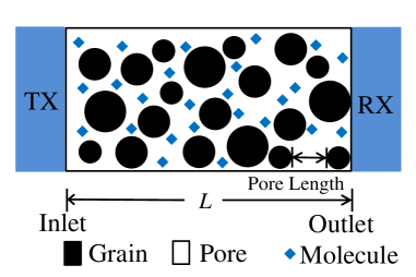
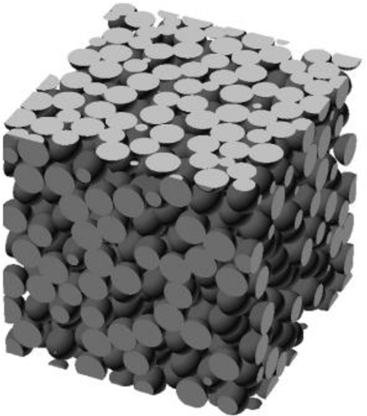
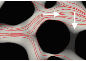
Figure 1: 1: A 2D sketch of the considered system model, where $L$ is the distance between the TX and RX. 1: A 3D sample of a PM [13]. 1: Illustration of molecular transport through a PM with heterogeneous advection [10], where the red lines represent streamlines of the laminar flow; the shading of the background denotes the flow velocity which decreases from light to dark; the horizontal arrow denotes transport of molecules over the length of a pore in streamwise direction; and the vertical arrow indicates transport of molecules across streamlines into low velocity zones in the wake of the solid grains. In 1 and 1, the grains are represented in grey and black, respectively.

We consider an MC system via the PM in a three-dimensional (3D) environment where the TX and the RX are located at the inlet and the outlet of the PM, respectively. A two-dimensional (2D) sketch of the considered system is given in Fig. 1 and a 3D sample of a PM is shown in Fig. 1. In a PM, pores and grains refer to its void and solid components, respectively. Grain size distribution and porosity (i.e., the ratio of the volume of voids over the total volume) affect the transport behavior in the PM. In the following, we detail the key steps of the considered system.

Modulation and Emission: A sequence of binary symbols is transmitted with $\textnormal{Pr}(X_{n}=1)=P_{1}$, where $X_{n}$ is the $n$th transmitted symbol. We consider the on-off keying modulation scheme with a fixed symbol slot length $T$, which is commonly adopted in MC literature, i.e., at the beginning of the $n$th symbol slot, the TX releases $N$ molecules if $X_{n}=1$; otherwise, no molecule is released. The TX uniformly releases the molecules over the cross section at the inlet of the PM. We note that the use of a binary sequence is expected in MC between nanomachines to exchange the amount of information required for executing complex collaborative tasks, e.g., disease detection [14], and binary symbols are easier to transmit than symbols that carry more bits of information.

Transport through the PM: We consider the PM filled with an incompressible fluid of viscosity $\mu$, moving with a mean velocity $\vec{v}_{m}$ oriented from the TX to the RX. Due to the small pore sizes, the flow is laminar (Reynolds number of the flow is negligible) and governed by the Stokes equation $\mu\nabla^{2}\vec{v}(\mathbf{a})=\nabla p(\mathbf{a})$ together with the incompressibility condition $\nabla\vec{v}(\mathbf{a})=0$, where $\nabla$ is the nabla operator, $\mathbf{a}$ denotes location, $\vec{v}$ is the velocity, and $p(\mathbf{a})$ is the pressure. The boundary conditions are of zero velocity (no-slip) on the surface of the solid grains, and periodic on the external boundaries, with a fixed pressure gradient along the mean flow direction. The resulting velocity field $\vec{v}$ is characterized by a chaotic heterogeneous structure. Mechanical entrapment of molecules may occur in PM when the molecules are too large to enter small pores [15]. Small molecules such as water and salt molecules can travel through PM, but large molecules such as polymer molecules will be trapped and accumulate in these small pores. Although these effects are not explicitly modelled here (they would, in fact, require a Lagrangian description of molecules as rigid bodies), a similar effect is here included when the flow velocity is high compared to molecular diffusion. The few molecules that diffuse into stagnant regions can get trapped for relatively long times before diffusing back into the main flow channels.

The molecular transport in the pores is due to molecular diffusion and the complex heterogeneous advection around solid grains, as shown in Fig. 1. The molecular concentration $c(\mathbf{a},t)$ is modeled by an advection-diffusion equation [16]:

$${\partial c(\mathbf{a},t)}/{\partial t}+\vec{v}(\mathbf{a})\nabla c(\mathbf{a},t)-D\nabla^{2}c(\mathbf{a},t)=0\,,$$ (1)

where $D$ is the constant diffusion coefficient, with a constant flux of molecules on the inlet and zero diffusive flux on all other boundaries. Although these equations are linear and relatively easy to solve, the complexity of the geometry makes the discretization and solution particularly cumbersome[8].

The Péclet number (Pe), which compares advective and diffusive transport over the whole PM length $L$, is given by $\textnormal{Pe}={|\vec{v}_{m}|L}/{D}$. Thanks to the interplay of these two phenomena, molecules not only are transported along the streamlines but also travel across streamlines, experiencing therefore a wide range of velocities, and possibly reaching stagnant zones in the wake of the solid grains. Molecules that enter these zones can remain there for some time before they escape and return into the mobile portion of the medium. The transport of molecules through PM may also be affected by electro-chemical effects. For example, molecules may contain polar groups, which will attach to the available polar points on the PM surface [15]. Depending on the PM surface net ionic charge, electrostatic attraction or repulsion would occur for ionic molecules, which enhance or reduce the ionic molecular adsorption on the surface of PM. For the tractability of the distribution of first arrival time of molecules, we do not consider electrical effects on molecular propagation.

Reception and Demodulation: We consider a RX that is mounted on the cross section at the outlet of the PM and is able to count the number of molecules that arrive. To decrease the complexity, we consider a fixed threshold-based demodulation rule at the RX: $Y_{n}=1$ if $N^{\textnormal{ob}}_{n}\geq\xi$; otherwise, $Y_{n}=0$, where $Y_{n}$ is the $n$th received symbol, $N^{\textnormal{ob}}_{n}$ is the number of molecules that arrive during the $n$th slot, and $\xi$ is a fixed threshold. The transmission and reception of multiple symbols is possible. The encoding function at the TX can be implemented by synthesizing logic gates [17]. A metabolic pathway of a biological cell can be synthesized into the TX to release specific molecules [18]. The computational processing at the RXs can be implemented based on [19, 20]. The time synchronization between the TX and the RXs can be implemented using various methods, e.g., a blind synchronization algorithm [21] and quorum sensing-based method [22].

III Performance Metrics

In this section, we present the analytical results of system performance metrics. To this end, we first analyze the (cumulative) breakthrough curve, i.e., the cumulative density function (CDF) of the first arrival time at the outlet of any molecule released from the inlet, which is used for characterizing molecular transport in the PM. This is given by [10]

$$F(t)\!=\!\frac{\int\!\int\!c(a_{1}\!=\!L,a_{2},a_{3},t)|\vec{v}(a_{1}=L,a_{2},a_{3})|da_{2}da_{3}}{\int\int|\vec{v}(a_{1}=L,a_{2},a_{3})|da_{2}da_{3}},\vspace{-4mm}$$ (2)

where $\mathbf{a}=\{a_{1},a_{2},a_{3}\}$ denotes location in Cartesian coordinates. The analytical expression for $F(t)$ is mathematically intractable, so we will rely on a numerical solution obtained by the full discretization of (1) and (2). For more details about numerical solvers, we refer the readers to [8].

If the TX and RX only partially cover the media inlet and outlet, then the breakthrough curve needs to be re-computed since the boundary conditions change and the dimension of the problem effectively increases (since the whole coverage case is effectively a one-dimensional system). More generally, when the TX and the RX are located arbitrarily in an open three-dimensional domain, one would need to consider a full non-diagonal and anisotropic dispersion tensor [6] and not only the longitudinal dispersion studied here. We expect that the difference between breakthrough curves with full and partial coverage, to resembles the difference between diffusion processes in one and more dimensions.

Remark 1

Assuming that the number of molecules arrived can be approximated as a Gaussian RV, we derive the mutual information $I$, throughput $C$, and error probability $Q$. Using particle-based simulation methods, [23, 24] have verified the accuracy of Gaussian approximation. According to the central limit theorem, the accuracy of this approximation improves as $N$ increases. Due to the space limitation, we present the derivation of statistical distributions of molecules arrived and system performance metrics in Appendix A.

We next discuss the diversity gain. Each molecule behaves independently and experiences different propagation paths. Thus, the channel can be seen as a multiple-input and multiple-output channel and the RX achieves diversity when $N$ molecules are released. Also, there is an optimal $\xi$ that minimizes error probability $Q$, i.e., $Q^{\ast}=\underset{\xi}{\text{min}}\;Q$, where $Q^{\ast}$ is the optimal error probability. We define the diversity gain as the exponentially decreasing rate of $Q^{\ast}$ as a function of increasing $N$. That is to say, if we can well approximate $Q^{\ast}$ with a form of $Q^{\ast}\approx\exp(-\alpha N+\beta)$, then $\alpha$ is the diversity gain. The assessment of the diversity gain of different channels indicates which channel is more sensitive to the increase in the number of molecules released, without the need for explicitly calculating the probability of error. Specifically, if a higher diversity gain is achieved, the channel is more sensitive. Thus, the evaluation of diversity gain provides information regarding the fundamental properties of different channels, which for example facilities the appropriate selection of the number of molecules released for MC system design. Since an explicit expression for $\alpha$ is mathematically intractable, we use a data-fitting method to obtain $\alpha$. The method will be detailed in Sec. IV. We note that a similar definition of $\alpha$ was studied in [11] for timing channels, but our method for evaluating $\alpha$ is different from [11].

For $P_{1}=\frac{1}{2}$, we have following corollaries on $Q$ and $I$:

Corollary 1

The optimal error probability converges to zero when the released number of molecules for symbol “1” tends to infinity, i.e., $\lim_{N\to\infty}Q^{\ast}=0$.

Corollary 2

The mutual information is bounded by $I\leq 1\,{\textnormal{bits}}/{\textnormal{slot}}$ and $I=1\,{\textnormal{bits}}/{\textnormal{slot}}$ is obtained if and only if $Q\to 0$.

Proof:

The proofs of Corollaries 1 and 2 are given in Appendices B and C, respectively. ∎

IV Numerical Results

In this section, we present numerical results to investigate the channel response and communication performance of MC via the PM. We consider the 3D sand-like PM described in [8, 10]. The medium was generated according to the characteristics of standard sand samples. Specifically, the PM is a cube of size $L=2{\textnormal{m}}\textnormal{m}$, which is of the size of a representative elementary volume in terms of the definition of volumetric porosity [6]. The typical porosity of many kinds of soils, e.g., gravel, sand, silt, and clay, is between $20\%$ and $50\%$, based on [25, 26, 27]. The typical grain diameter for medium sand is between $0.25\,{\textnormal{m}}\textnormal{m}$ and $0.5\,{\textnormal{m}}\textnormal{m}$ [28]. We consider the porosity of $35\%$ and the grain diameter of $0.277\,{\textnormal{m}}\textnormal{m}$, which are within the normal range for sand samples. The grain size distribution follows a Weibull distribution with Weibull parameter $k=7$. We also consider $n=10$ symbols are transmitted with $P_{1}=\frac{1}{2}$. The other parameters are given in Table I. With these parameters, [10] numerically solved (1) and (2), obtaining the values of $F(t)$ for $\textnormal{Pe}=3,30,300,1000$. The results in the following figures are obtained based on this simulation data. In Fig 4, Fig 6, and Table II, we assume that $N^{\textnormal{ob}}_{n}$ is a Poisson RV since we consider $N\leq 100$. In Fig 5, we assume $N^{\textnormal{ob}}_{n}$ is a Gaussian RV since we consider $N=10^{5}$.

TABLE I: Environmental Parameters

Parameter	Symbol	Value
Length of PM	$L$	$2\,{\textnormal{m}}\textnormal{m}$
Number of grains	$\phi$	$2\times 10^{3}$
Average grain diameter	$\overline{d}$	$0.277\,{\textnormal{m}}\textnormal{m}$
Characteristic pore length (estimated)	$\ell_{0}$	$0.277\,{\textnormal{m}}\textnormal{m}$
Mean velocity	$|\vec{v}_{m}|$	$5.73\times 10^{-6}\textnormal{m}/\textnormal{s}$

In order to provide more insights, we compare with a one-dimensional (1D) diffusive FS channel with a flow oriented from the TX to the RX, which is referred to as the “FS channel” in the following for brevity. This is because the PM channel is effectively a 1D channel due to the TX and RX covering the entire inlet and outlet. The probability density function (PDF) of the first arrival time at $a_{1}=L$ in the FS channel is given by $f(t)=\frac{L}{\sqrt{4\pi Dt^{3}}}\exp(-\frac{(|\vec{v}_{m}|t-L)^{2}}{4Dt})$ [29]. For this FS channel, we consider the same parameter values as those for the PM channel for the fairness of our comparison.

IV-A Channel Response

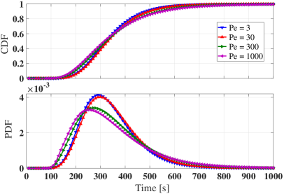
Figure 2: The CDF and PDF $f(t)$ of the arrival time of the molecule versus time $t$ in the PM channel for different Pe.

In Fig. 2, we show the arrival time distribution in the PM channel. The PDF curves are obtained by numerically evaluating the derivative of $F(t)$. Firstly, for all Pe, $F(t)\to 1$ as $t\to\infty$, which means that all molecules released will eventually arrive at the RX. This is because no flow is going out of the lateral directions and no molecule can escape from the lateral directions by advection nor by diffusion. Secondly, when Pe is smaller, the CDF converges more quickly to 1, meaning that less molecules stay trapped in the PM.

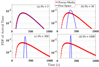
Figure 3: The PDF $f(t)$ of the arrival time of the molecule versus time in the PM and FS channels for different Pe.

In Fig. 3, we compare the arrival time PDF in the PM channel with that in the FS channel. Interestingly, when Pe is 3, the PDF curve for the PM is similar to that for FS. This is because the fact that molecular diffusion is fairly large, causing particles to uniformly sample the velocity space, and resulting in an overall transport that can be conveniently described as a single advection-diffusion channel. Secondly, PM channel behavior is much less sensitive to Pe than in the FS channel. This is due to molecules entering dead-end pores or stagnant regions, and taking a long time to escape in the PM. For FS, when Pe is larger, since there are no such regions, the only effect is a more dominant advection than the diffusion, thus FS channel behavior is more sensitive to larger Pe. Importantly, as Pe increases (e.g., larger molecules with smaller diffusion coefficient), the peak value of the PDF curve for the FS channel increases, while that for the PM model decreases (as seen in Fig. 2), i.e., the PDF curve for the FS channel becomes narrower but the PDF curve for the PM becomes longer. This is because for the PM, the particles travel in all directions through the complex network of pores, thus generating a much larger “longitudinal dispersivity”, i.e, a higher equivalent diffusion in the longitudinal direction, proportional to Pe[8]. This means that, as Pe increases, the ISI of the PM channel increases but ISI of the FS channel decreases. Based on this, for the PM channel we expect the error performance and mutual information would become worse when Pe increases, which will be verified by the observations in Fig. 4.

IV-B Performance Evaluation

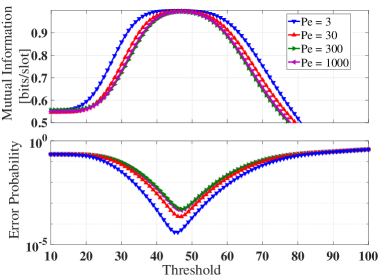
Figure 4: The average mutual information $I$ and the average error probability $Q$ of the MC system via the PM versus the threshold $\xi$ for different Pe: $\textnormal{Pe}=3,30,300,1000$. $N=100$ and $T=400\,\textnormal{s}$.

In Fig. 4, we show the average mutual information and the average error probability of the PM channel. Firstly, when $\xi=45$, $I$ is maximal (i.e., $I=1\,{\textnormal{bits}}/{\textnormal{slot}}$) and $Q$ is minimal, which numerically validates Corollary 2. Secondly, the average mutual information is smaller and the error probability is higher as Pe increases. This is because when Pe is higher, the tail of the channel response of the PM is longer, i.e., larger ISI, as we observed in Figs. 2 and 3.

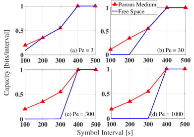
Figure 5: The throughput $C$ of the MC system via the PM and FS channels versus the symbol slot $T$ with $N=10^{5}$ for different Pe: (a) $\textnormal{Pe}=3$, (b) $\textnormal{Pe}=30$, (c) $\textnormal{Pe}=300$, and (d) $\textnormal{Pe}=1000$.

In Fig. 5, we show the throughput of the PM and FS channels. Firstly, for both channels and all Pe, $C$ increases as $T$ increases and $C=1\,{\textnormal{bits}}/{\textnormal{slot}}$ is achieved when $T\geq 400\,\textnormal{s}$. This is because of a very small probability that a molecule arrives at $t\geq 400\,\textnormal{s}$, as observed in Fig. 3. Secondly, the difference of $C$ between the PM and FS channels when $T\leq 300\,\textnormal{s}$ becomes larger as Pe increases. This is because in Fig. 3, when Pe increases, the PM and FS channels diverge.

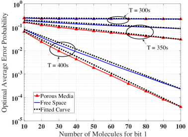
Figure 6: The optimal average error probability $Q^{\ast}$ of the MC system versus the number of molecules $N$ released for bit “1” for different symbol slots: $T=300\,\textnormal{s}$, $T=350\,\textnormal{s}$, and $T=400\,\textnormal{s}$ with $\textnormal{Pe}=3$.

TABLE II: Diversity Gain

Diversity Gain $\alpha$		$\textnormal{Pe}=3$	$\textnormal{Pe}=30$	$\textnormal{Pe}=300$	$\textnormal{Pe}=1000$
$T=300\,\textnormal{s}$	FS	0.0013	0.0055	0	0
	PM	0.0009	0.0013	0.0010	0.0008
$T=350\,\textnormal{s}$	FS	0.0089	0.0032	0.0048	0.0094
	PM	0.0186	0.0109	0.0144	0.0184
$T=400\,\textnormal{s}$	FS	0.0651	0.2689	0.8334	0.9487
	PM	0.0822	0.0651	0.0569	0.0585

In Fig. 6, we plot the optimal average error probability versus the number of molecules released for bit “1” for different symbol slots. The considered symbol slots are around the detection time that maximizes the PM and FS channel responses based on Fig. 3. Firstly, $Q^{\ast}$ decreases when $N$ increases. We then see that error probability curves can be well approximated by the fitted curves, $Q^{\ast}\approx\exp(-\alpha N+\beta)$, where $\alpha$ and $\beta$ are obtained by solving $Q^{\ast}|_{N=10}=\exp(-\alpha 10+\beta)$ and $Q^{\ast}|_{N=100}=\exp(-\alpha 100+\beta)$. Thus, we can use the diversity gain $\alpha$ to quantify the decrease rate of $Q^{\ast}$ as $N$ increases. We present $\alpha$ for different $T$ and Pe in Table II. We find that the PM achieves higher $\alpha$ than the FS channel for any Pe with $T=350\,\textnormal{s}$. This is because the decrease rate of $Q^{\ast}$ is affected by ISI. The PM has less ISI than the FS channel for these parameter values, based on the tails of the PDF curves of arrival time shown in Fig. 3.

V Conclusion

We for the first time considered MC via a realistic PM channel, modeled as a 3D complex pore structure. Using fully resolved computational fluid dynamics results for the arrival time distribution, we explored the differences in channel characteristics between PM and FS channels and their impact on communication performance metrics (i.e., throughput, mutual information, error probability, and diversity gain) in both channels. Our results suggest that the reliability of a PM channel can be improved by decreasing Pe, while opposite trends for a FS channel.

Although the parameters (e.g., porosity, size, and topology) of different types of natural PM vary widely, their fundamental channel characteristics, i.e., the changing trends in the molecular arrival time distribution as Pe changes, are the same. This is because the key characteristic of molecular transport through the PM channel is that molecules may become trapped in the vicinity of solid grains, therefore taking some time to exit and causing non-trivial anomalous transport phenomena, such as long tails in the arrival time distributions. Our results reveal such changing trends in the molecular arrival time distribution and its impact on the different performance metrics of PM as Pe changes. These results provide useful guidelines for designing the optimal MC system through PM and predicting the system communication performance in a practical biological environment where Pe may change due to the instability of temperature and diffusion coefficients. In our future work, we could analytically derive the arrival time distribution of a simplified, yet realistic, PM channel.

Appendix A Derivation of Performance metrics

Due to the transport delay experienced by the molecules that arrive at the RX, the RX may receive the molecules released from the current and all previous symbol slots. Based on (2), we obtain the probability that the molecule being released in the $k$th symbol slot arrives during the $n$th symbol slot, i.e., $F((n-k+1)T)-F((n-k)T)$. We denote $N^{\textnormal{ob}}_{n,k}$ as the number of molecules that arrive during the $n$th slot that were released at the beginning of the $k$th symbol slot. We then have $N^{\textnormal{ob}}_{n}=\sum_{k=1}^{n}N^{\textnormal{ob}}_{n,k}=\sum_{k=1}^{n-1}N^{\textnormal{ob}}_{n,k}+N^{\textnormal{ob}}_{n,n}$, where $\sum_{k=1}^{n-1}N^{\textnormal{ob}}_{n,k}$ is the ISI and $N^{\textnormal{ob}}_{n,n}$ is from the intended molecular signal. Since the molecules released in a given slot are transported independently and have the same probability to arrive during the $n$th slot, $N^{\textnormal{ob}}_{n,k}$ follows a binomial distribution, i.e.,

$$N^{\textnormal{ob}}_{n,k}\sim X_{k}B(N,F((n-k+1)T)-F((n-k)T)).$$ (3)

We note that modeling $N^{\textnormal{ob}}_{n,k}$ with the binomial distribution makes the analysis of $N^{\textnormal{ob}}_{n}$ cumbersome, since a sum of Binomial random variables (RVs) is not in general a Binomial RV. Fortunately, $N^{\textnormal{ob}}_{n,k}$ can be accurately approximated by a Poisson distribution when $N$ is large and $F((n-k+1)T)-F((n-k)T)$ is small with $NF((n-k+1)T)-F((n-k)T)<10$. By doing so, we rewrite $N^{\textnormal{ob}}_{n,k}$ as

$$N^{\textnormal{ob}}_{n,k}\sim X_{k}P(N(F((n-k+1)T)-F((n-k)T))).$$ (4)

The sum of independent Poisson RVs is also a Poisson RV whose mean is the sum of the means of the individual Poisson RVs. As such, we have

$$N^{\textnormal{ob}}_{n}\sim P\left(\gamma\right).$$ (5)

where $\gamma=N\sum_{k=1}^{n}X_{k}(F((n-k+1)T)-F((n-k)T))$. In the following, we aim to derive $\textnormal{Pr}(N^{\textnormal{ob}}_{n}<\xi)$, since it lays the foundation for deriving all performance metrics in this paper. Based on (5), the CDF of the Poisson RV $N^{\textnormal{ob}}_{n}$ is written as

$$\textnormal{Pr}(N^{\textnormal{ob}}_{n}<\xi|X_{1:n})=\sum_{j=1}^{\xi}\frac{\exp(-\gamma)\gamma^{j}}{j!}.$$ (6)

We note that the the large number of summation terms in (6) makes (6) have very high computational complexity when $\xi$ is large. To facilitate the evaluation when $\xi$ is large, we further approximate $N^{\textnormal{ob}}_{n}$ as a Gaussian RV as follows:

$$N^{\textnormal{ob}}_{n}\sim N(\gamma,\gamma),$$ (7)

where $\gamma=N\sum_{k=1}^{n}X_{k}(F((n-k+1)T)-F((n-k)T))$. The Gaussian approximation for $N^{\textnormal{ob}}_{n}$ in (7) is accurate when $\gamma>10$. We define $X_{1:n}=\{X_{1},X_{2},\ldots,X_{n}\}$ as the subsequence of the symbols transmitted by the TX. Based on (7), we obtain the conditional CDF of the Gaussian RV $N^{\textnormal{ob}}_{n}$ for the given $X_{1:n}$ as

$$\textnormal{Pr}(N^{\textnormal{ob}}_{n}<\xi|X_{1:n})=\frac{1}{2}\left(1+\operatorname{erf}\left(\frac{\xi-0.5-\gamma}{\sqrt{2\gamma}}\right)\right),$$ (8)

where $0.5$ is a continuity correction. Using (6) or (8), we obtain the following conditional probabilities for the given $X_{1:n-1}$ as:

$$\textnormal{Pr}(Y_{n}=0|X_{n}=0,X_{1:n-1})=\textnormal{Pr}(N^{\textnormal{ob}}_{n}<\xi|X_{n}=0,X_{1:n-1}),$$ (9)

$$\textnormal{Pr}(Y_{n}=1|X_{n}=0,X_{1:n-1})$$

$$= \;1-\textnormal{Pr}(N^{\textnormal{ob}}_{n}<\xi|X_{n}=0,X_{1:n-1}),$$ (10)

$$\textnormal{Pr}(Y_{n}=0|X_{n}=1,X_{1:n-1})=\textnormal{Pr}(N^{\textnormal{ob}}_{n}<\xi|X_{n}=1,X_{1:n-1}),$$ (11)

and

$$\textnormal{Pr}(Y_{n}=1|X_{n}=1,X_{1:n-1})$$

$$= \;1-\textnormal{Pr}(N^{\textnormal{ob}}_{n}<\xi|X_{n}=1,X_{1:n-1}).$$ (12)

Using (9)-(A), we first derive the conditional mutual information between channel input and output and the conditional symbol error probability given the subsequence of the previous symbols transmitted by the TX, $X_{1:n-1}$. To assess the overall system communication performance when transmitting different sequences of symbols, we then evaluate the average mutual information and the average symbol error probability over all realizations of $X_{1:n}$ and all symbol slots from 1 to $n$.

Mutual Information: We derive the conditional mutual information between $X_{n}$ and $Y_{n}$ for the given $X_{1:n-1}$ as

$$I(X_{n};Y_{n}|X_{1:n-1})$$

$$= \;H(Y_{n}|X_{1:n-1})-H(Y_{n}|X_{n},X_{1:n-1})~{}{{\textnormal{bits}}/{\textnormal{slot}}}.$$ (13)

where $H(\cdot)$ is the entropy. We derive $H(Y_{n})$ as

$$\;H(Y_{n}|X_{1:n-1})$$

$$= -\textnormal{Pr}(Y_{n}=0|X_{1:n-1})\log_{2}\textnormal{Pr}(Y_{n}=0|X_{1:n-1})$$

$$-\textnormal{Pr}(Y_{n}=1|X_{1:n-1})\log_{2}\textnormal{Pr}(Y_{n}=1|X_{1:n-1}),$$ (14)

where $\textnormal{Pr}(Y_{n}=0|X_{1:n-1})$ and $\textnormal{Pr}(Y_{n}=1|X_{1:n-1})$ are written as

$$\textnormal{Pr}(Y_{n}=0|X_{1:n-1})= \;(1-P_{1})\textnormal{Pr}(Y_{n}=0|X_{n}=0,X_{1:n-1})$$

$$+P_{1}\textnormal{Pr}(Y_{n}=0|X_{n}=1,X_{1:n-1})$$ (15)

and

$$\textnormal{Pr}(Y_{n}=1|X_{1:n-1})= \;(1-P_{1})\textnormal{Pr}(Y_{n}=1|X_{n}=0,X_{1:n-1})$$

$$+P_{1}\textnormal{Pr}(Y_{n}=1|X_{n}=1,X_{1:n-1}),$$ (16)

respectively. We derive $H(Y_{n}|X_{n},X_{1:n-1})$ as

$$H(Y_{n}|X_{n},X_{1:n-1})= \;(1-P_{1})H(Y_{n}|X_{n}=0,X_{1:n-1})$$

$$+P_{1}H(Y_{n}|X_{n}=1,X_{1:n-1}),$$ (17)

where $H(Y_{n}|X_{n}=0,X_{1:n-1})$ and $H(Y_{n}|X_{n}=1,X_{1:n-1})$ are given by

$$H(Y_{n}|X_{n}=0,X_{1:n-1})$$

$$= -\textnormal{Pr}(Y_{n}=0|X_{n}=0,X_{1:n-1})$$

$$\times\log_{2}\textnormal{Pr}(Y_{n}=0|X_{n}=0,X_{1:n-1})$$

$$-\textnormal{Pr}(Y_{n}=1|X_{n}=0,X_{1:n-1})$$

$$\times\log_{2}\textnormal{Pr}(Y_{n}=1|X_{n}=0,X_{1:n-1}),$$ (18)

and

$$H(Y_{n}|X_{n}=1,X_{1:n-1})$$

$$= -\textnormal{Pr}(Y_{n}=0|X_{n}=1,X_{1:n-1})$$

$$\times\log_{2}\textnormal{Pr}(Y_{n}=0|X_{n}=1,X_{1:n-1})$$

$$-\textnormal{Pr}(Y_{n}=1|X_{n}=1,X_{1:n-1})$$

$$\times\log_{2}\textnormal{Pr}(Y_{n}=1|X_{n}=1,X_{1:n-1}),$$ (19)

respectively. We finally derive the average mutual information over all realizations of $X_{1:n-1}$ and all symbol slots from 1 to $n$ as

$$I=\frac{1}{n}\sum_{k=1}^{n}\frac{\sum_{X_{1:k-1}\in\Psi_{k}}I(X_{k};Y_{k}|X_{1:k-1})}{2^{k-1}}~{}{{\textnormal{bits}}/{\textnormal{slot}}},$$ (20)

where $\Psi_{k}$ is a set that includes all realizations of $X_{1:k-1}$.

Throughput: We derive the throughput, i.e., the maximal average mutual information, as

$$C=\underset{\xi}{\text{max}}~{}\frac{1}{n}\sum_{k=1}^{n}\frac{\sum_{X_{1:k-1}\in\Psi_{k}}I(X_{k};Y_{k}|X_{1:k-1})}{2^{k-1}}~{}{{\textnormal{bits}}/{\textnormal{slot}}}.$$ (21)

Error Probability: We derive the symbol error probability in the $n$th slot for the given $X_{1:n-1}$ as

$$Q[n|X_{1:n-1}]= \;(1-P_{1})\textnormal{Pr}(Y_{n}=1|X_{n}=0,X_{1:n-1})$$

$$+P_{1}\textnormal{Pr}(Y_{n}=0|X_{n}=1,X_{1:n-1}).$$ (22)

We derive the average symbol error probability over all realizations of $X_{1:n-1}$ and all symbol slots from 1 to $n$ as

$$Q=\frac{1}{n}\sum_{k=1}^{n}\frac{\sum_{X_{1:k-1}\in\Psi_{k}}Q[k|X_{1:k-1}]}{2^{k-1}}.$$ (23)

Appendix B Proof of Corollary 1

Since $Q$ is the sum of $Q[n|X_{1:n-1}]$ based on (23), we need to prove that $Q^{\ast}[n|X_{1:n-1}]\to 0$ when $N\to\infty$, where $Q^{\ast}[n|X_{1:n-1}]=\underset{\xi}{\text{min}}\;Q[n|X_{1:n-1}]$. Assuming $P_{1}=\frac{1}{2}$, we first rewrite (A) as

$$Q[n|X_{1:n-1}]= \;\frac{1}{2}+\frac{1}{4}\left[\operatorname{erf}\left(\frac{\xi-0.5-(N(Y_{1}+Y_{2}))}{\sqrt{2(N(Y_{1}+Y_{2}))}}\right)\right.$$

$$\left.-\operatorname{erf}\left(\frac{\xi-0.5-NY_{2}}{\sqrt{2NY_{2}}}\right)\right],$$ (24)

where $Y_{1}=(F(T)-F(0))$ and $Y_{2}=\sum_{k=1}^{n-1}X_{k}(F((n-k+1)T)-F((n-k)T))$. We then obtain the optimal $\xi$ that minimizes $Q[n|X_{1:n-1}]$. To this end, we take the first derivative of (B) with respect to $\xi$ and solve the resultant equation to derive the optimal $\xi$ that minimizes $Q[n|X_{1:n-1}]$ as

$$\xi^{\ast}[n|X_{1:n-1}]=\frac{NY_{1}}{\ln\left({(Y_{1}+Y_{2})}/{Y_{2}}\right)}.$$ (25)

Substituting (25) into (B), we write the optimal error probability $Q[n|X_{1:n-1}]$ as

$$Q^{\ast}[n|X_{1:n-1}]= \frac{1}{2}\!+\!\frac{1}{4}\!\left[\operatorname{erf}\!\left(\frac{\sqrt{N}\!A}{\sqrt{2(Y_{1}+Y_{2})}}\right)\right.$$

$$\left.-\operatorname{erf}\left(\frac{\sqrt{N}\!B}{\sqrt{2Y_{2}}}\right)\right],$$ (26)

where

$$A=\left(\frac{Y_{1}}{\ln\left({(Y_{1}+Y_{2})}/{Y_{2}}\right)}\!-\!(Y_{1}+Y_{2})\right)$$ (27)

and

$$B=\left(\frac{Y_{1}}{\ln\left({(Y_{1}+Y_{2})}/{Y_{2}}\right)}\!-\!Y_{2}\right).$$ (28)

If we can prove $A<0$ and $B>0$, then we have

$$\lim_{N\to\infty}Q^{\ast}[n|X_{1:n-1}]= \frac{1}{2}\!+\!\frac{1}{4}\!\left[\operatorname{erf}\!\left(-\infty\right)\right.\left.-\operatorname{erf}\left(\infty\right)\right]=0.$$ (29)

We now prove $A<0$ and $B>0$. Since $Y_{1}>0$ and $Y_{2}>0$, it is reasonably to assume $Y_{1}=xY_{2}$, $x>0$. Using $Y_{1}=xY_{2}$, we simplify the conditions $A<0$ and $B>0$ to $x/(1+x)-\ln(1+x)<0$ and $x-\ln(1+x)>0$, respectively. We find that $g(x)=x/(1+x)-\ln(1+x)$ is a decreasing function and $f(x)=x-\ln(1+x)$ is an increasing function with respect to $x$ since $g^{\prime}(x)=-x/(1+x)^{2}<0$ and $f^{\prime}(x)=1-1/(1+x)>0$ if $x>0$. By inspection, we also find $g(x)=0$ and $f(x)=0$ at $x=0$. Thus, we have $g(x)<0$ and $f(x)>0$ for $x>0$, which means $A<0$ and $B>0$. Thus, we verify that $Q^{\ast}[n|X_{1:n-1}]\to 0$ when $N\to\infty$, which completes the proof.

Appendix C Proof of Corollary 2

We first prove $I(X_{n};Y_{n}|X_{1:n-1})\leq 1\,{\textnormal{bits}}/{\textnormal{slot}}$. As per the Shannon entropy of probability distributions for single parties, we have $I(X_{n};Y_{n}|X_{1:n-1})\leq\text{min}\{H(X_{n}|X_{1:n-1}),H(Y_{n}|X_{1:n-1})\}$. Based on definition of entropy, the maximal $H(X_{n}|X_{1:n-1})$ and $H(Y_{n}|X_{1:n-1})$ is $1\,{\textnormal{bits}}/{\textnormal{slot}}$ when $\textnormal{Pr}(X_{1}=0)=P_{1}=\frac{1}{2}$ and $\textnormal{Pr}(Y_{1}=0)=\frac{1}{2}$. Thus, the mutual information is bounded by $I(X_{n};Y_{n}|X_{1:n-1})\leq 1\,{\textnormal{bits}}/{\textnormal{slot}}$.

We then prove that $Q\to 0$ is a sufficient condition for $I(X_{n};Y_{n}|X_{1:n-1})=1\,{\textnormal{bits}}/{\textnormal{slot}}$. Based on (A), $Q[n|X_{1:n-1}]\to 0$ means $\textnormal{Pr}(Y_{n}=1|X_{n}=0,X_{1:n-1})\to 0$ and $\textnormal{Pr}(Y_{n}=0|X_{n}=1,X_{1:n-1})\to 0$. Applying these two expressions to (A) and (A), we obtain $I(X_{n};Y_{n}|X_{1:n-1})=1\,{\textnormal{bits}}/{\textnormal{slot}}$, which proves $Q\to 0$ is a sufficient condition. We finally prove that $Q\to 0$ is a necessary condition for $I(X_{n};Y_{n}|X_{1:n-1})=1\,{\textnormal{bits}}/{\textnormal{slot}}$. Since $H(Y_{n}|X_{1:n-1})\leq 1$ and $H(Y_{n}|X_{n},X_{1:n-1})\geq 0$, thus $I(X_{n};Y_{n}|X_{1:n-1})=1\,{\textnormal{bits}}/{\textnormal{slot}}$ is achieved only when $H(Y_{n}|X_{1:n-1})=1$ and $H(Y_{n}|X_{n},X_{1:n-1})=0$. $H(Y_{n}|X_{n},X_{1:n-1})=0$ means $H(Y_{n}|X_{n}=0,X_{1:n-1})=0$ and $H(Y_{n}|X_{n}=1,X_{1:n-1})=0$ based on (A). There are four cases leading to $H(Y_{n}|X_{n}=0,X_{1:n-1})=0$ and $H(Y_{n}|X_{n}=1,X_{1:n-1})=0$ including:

1. $\textnormal{Pr}(Y_{n}=0|X_{n}=1,X_{1:n-1})=0$ and $\textnormal{Pr}(Y_{n}=1|X_{n}=0,X_{1:n-1})=0$;

2. $\textnormal{Pr}(Y_{n}=0|X_{n}=1,X_{1:n-1})=1$ and $\textnormal{Pr}(Y_{n}=1|X_{n}=0,X_{1:n-1})=0$;

3. $\textnormal{Pr}(Y_{n}=0|X_{n}=1,X_{1:n-1})=0$ and $\textnormal{Pr}(Y_{n}=1|X_{n}=0,X_{1:n-1})=1$;

4. $\textnormal{Pr}(Y_{n}=0|X_{n}=1,X_{1:n-1})=1$ and $\textnormal{Pr}(Y_{n}=1|X_{n}=0,X_{1:n-1})=1$.

Since case 4) does not satisfy $\textnormal{Pr}(Y_{n}=0|X_{n}=1,X_{1:n-1})+\textnormal{Pr}(Y_{n}=1|X_{n}=0,X_{1:n-1})\leq 1$, case 4) is not valid. Moreover, cases 2) and 3) result in $\textnormal{Pr}(Y_{n}=0|X_{1:n-1})=1$ and $\textnormal{Pr}(Y_{n}=1|X_{1:n-1})=1$, respectively, which leads to $H(Y_{n}|X_{1:n-1})=0$. Thus, they are not valid either. We note that only case 1) satisfies both $H(Y_{n}|X_{1:n-1})=1$ and $H(Y_{n}|X_{n},X_{1:n-1})=0$ and case 1) leads to $Q\to 0$. Thus, $Q\to 0$ is a necessary condition. Therefore, we prove $Q\to 0$ is a sufficient and necessary condition for $I(X_{n};Y_{n}|X_{1:n-1})=1\,{\textnormal{bits}}/{\textnormal{slot}}$.

References

- [1] T. Nakano et al., “Molecular communication for nanomachines using intercellular calcium signaling,” in Proc. IEEE NANO 2005, Aug. 2005, pp. 478–481.
- [2] T. Nakano, Y. Okaie, and J. Liu, “Channel model and capacity analysis of molecular communication with brownian motion,” IEEE Commun. Lett., vol. 16, no. 6, pp. 797–800, Jun. 2012.
- [3] W. Guo et al., “Molecular versus electromagnetic wave propagation loss in macro-scale environments,” IEEE Trans. Mol. Bio. Multi-Scale Commun., vol. 1, no. 1, pp. 18–25, Aug. 2015.
- [4] B. E. Rittmann, “The significance of biofilms in porous media,” Water Resources Res., vol. 29, no. 7, pp. 2195–2202, Jul. 1993.
- [5] C. Perego and R. Millini, “Porous materials in catalysis: Challenges for mesoporous materials,” Chem. Soc. Rev., vol. 42, pp. 3956–3976, Nov. 2012.
- [6] J. Bear, Dynamics of fluids in porous media. New York: American Elsevier Pub. Co., 2013.
- [7] A. E. Scheidegger, “General theory of dispersion in porous media,” J. Geophysical Research, vol. 66, no. 10, pp. 3273–3278, Oct. 1961.
- [8] M. Icardi, G. Boccardo, D. Marchisio, T. Tosco, and R. Sethi, “Pore-scale simulation of fluid flow and solute dispersion in three-dimensional porous media,” Phys. Rev. E, vol. 90, no. 1, pp. 1–13, Jul. 2014.
- [9] E. Crevacore et al., “Recirculation zones induce non-fickian transport in three-dimensional periodic porous media,” Phys. Rev. E, vol. 94, no. 5, pp. 1–12, Nov. 2016.
- [10] M. Dentz, M. Icardi, and J. J. Hidalgo, “Mechanisms of dispersion in a porous medium,” J. Fluid Mechanics, vol. 841, pp. 851–882, Apr. 2018.
- [11] Y. Murin, N. Farsad, M. Chowdhury, and A. Goldsmith, “Exploiting diversity in one-shot molecular timing channels via order statistics,” IEEE Trans. Mol. Bio. Multi-Scale Commun., accepted to appear.
- [12] W. Haselmayr, S. M. H. Aejaz, A. T. Asyhari, A. Springer, and W. Guo, “Transposition errors in diffusion-based mobile molecular communication,” IEEE Commun. Lett., vol. 21, no. 9, pp. 1973–1976, Sep. 2017.
- [13] C. Chueh et al., “Effective conductivity in random porous media with convex and non-convex porosity,” Int. J. Heat and Mass Transfer, vol. 71, pp. 183–188, Apr. 2014.
- [14] M. Kuscu, E. Dinc, B. A. Bilgin, H. Ramezani, and Ö. B. Akan, “Transmitter and receiver architectures for molecular communications: A survey on physical design with modulation, coding and detection techniques,” CoRR, vol. abs/1901.05546, 2019. [Online]. Available: http://arxiv.org/abs/1901.05546
- [15] S. Al-Hajri, S. M. Mahmood, H. Abdulelah, and S. Akbari, “An overview on polymer retention in porous media,” Energies, vol. 11, no. 10, pp. 1–19, Oct. 2018.
- [16] A. Bejan, Convection Heat Transfer, 4th ed. New York, NY: Wiley, 2013.
- [17] T. S. Moon, C. Lou, A. Tamsir, B. C. Stanton, and C. A. Voigt, “Genetic programs constructed from layered logic gates in single cells,” Nat., vol. 491, no. 7423, pp. 249–253, Nov. 2012.
- [18] M.-T. Chen and R. Weiss, “Artificial cell-cell communication in yeast saccharomyces cerevisiae using signaling elements from arabidopsis thaliana,” Nat. Biotechnol., vol. 23, no. 12, pp. 1551–1555, Dec. 2005.
- [19] U. Pischel, “Chemical approaches to molecular logic elements for addition and subtraction,” Angew. Chem. Int. Ed., vol. 46, no. 22, pp. 4026–4040, May 2007.
- [20] A. P. de Silva and S. Uchiyama, “Molecular logic and computing,” Nature Nanotech., vol. 2, no. 7, pp. 399–410, Jul. 2007.
- [21] H. ShahMohammadian, G. G. Messier, and S. Magierowski, “Blind synchronization in diffusion-based molecular communication channels,” IEEE Commun. Lett., vol. 17, no. 11, pp. 2156–2159, Nov. 2013.
- [22] S. Abadal and I. F. Akyildiz, “Bio-inspired synchronization for nanocommunication networks,” in Proc. IEEE GLOBECOM, Dec. 2011, pp. 1–5.
- [23] A. Noel, K. C. Cheung, R. Schober, D. Makrakis, and A. Hafid, “Simulating with accord: Actor-based communication via reaction–diffusion,” Nano Commun. Networks, vol. 11, pp. 44–75, Mar. 2017.
- [24] H. B. Yilmaz, C.-B. Chae, B. Tepekule, and A. E. Pusane, “Arrival modeling and error analysis for molecular communication via diffusion with drift,” in Proc. ACM NANOCOM 2015, Sep. 2015, pp. 1–6.
- [25] B. M. Das, Advanced Soil Mechanics, 3rd ed. London, UK: Taylor & Francis, 2008.
- [26] “Characteristic coefficients of soils,” Association of Swiss Road and Traffic Engineers, Standard.
- [27] B. Hough, Basic soil engineering. New York, NY: Ronald Press Company, 1969.
- [28] R. L. Folk, “A review of grain-size parameters,” Sedimentology, vol. 6, no. 2, pp. 73–93, Mar. 1966.
- [29] J. Crank, The mathematics of diffusion, 2nd ed. Oxford University, 1975.
Supplementary Information