Bow shocks, bow waves, and dust waves. I. Strong coupling limit

Abstract

Dust waves and bow waves result from the action of a star’s radiation pressure on a stream of dusty plasma that flows past it. They are an alternative mechanism to hydrodynamic bow shocks for explaining the curved arcs of infrared emission seen around some stars. When gas and grains are perfectly coupled, for a broad class of stellar parameters, wind-supported bow shocks predominate when the ambient density is below $100\text{\,}\mathrm{c}\mathrm{m}^{-3}$. At higher densities radiation-supported bow shells can form, tending to be optically thin bow waves around B stars, or optically thick bow shocks around early O stars. For OB stars with particularly weak stellar winds, radiation-supported bow shells become more prevalent.

1 Introduction

Curved emission arcs around stars (e.g., Gull & Sofia, 1979) are often interpreted as bow shocks, due to a supersonic hydrodynamic interaction between the star’s wind and an external stream. This stream may be due to the star’s own motion or to an independent flow, such as an H ii region in the champagne phase (Tenorio-Tagle, 1979), or another star’s wind (Canto et al., 1996). However, an alternative interpretation in some cases may be a radiation-pressure driven bow wave, as first proposed by van Buren & McCray (1988, §vi). In this scenario (see Fig. 1), photons emitted by the star are absorbed by dust grains in the incoming stream, with the resultant momentum transfer being sufficient to decelerate and deflect the grains within a certain distance from the star, forming a dust-free, bow-shaped cavity with an enhanced dust density at its edge.

Two regimes are possible, depending on the strength of coupling between the gas (or plasma) and the dust. In the strong-coupling regime, gas–grain drag decelerates the gas along with the dust. If the stream is optically thin to the star’s ultraviolet radiation, then the deceleration occurs gradually over a range of radii, forming a relatively thick shell. On the other hand, if the stream is optically thick, then a shocked gas shell forms in a similar fashion to the wind-driven bow shock case, except internally supported by trapped radiation instead of shocked stellar wind. In the weak-coupling regime, the gas stream is relatively unaffected and the dust temporarily decouples to form a dust-only shell. This second case has recently been studied in detail in the context of the interaction of late O-type stars (some of which have very weak stellar winds) with dusty photoevaporation flows inside H ii regions (Ochsendorf et al., 2014b; Ochsendorf et al., 2014a; Ochsendorf & Tielens, 2015). We follow the nomenclature proposed by Ochsendorf et al. (2014a), in which dust wave refers to the weak coupling case and bow wave to the strong coupling case. More complex, hybrid scenarios are also possible, such as that studied by van Marle et al. (2011), where a hydrodynamic bow shock forms, but the larger dust grains that accompany the stellar wind pass right through the shocked gas shell, and form their own dust wave at a larger radius.

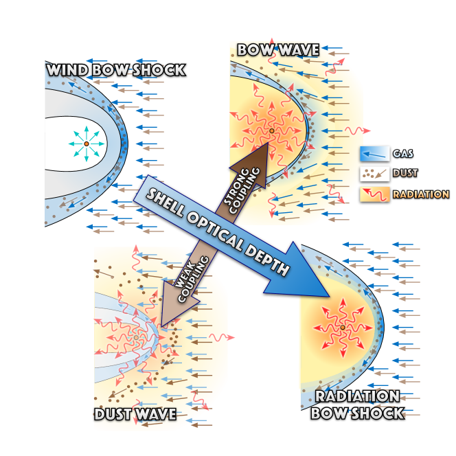
Figure 1: Regimes in the supersonic interaction of a luminous star with its environment. When radiation effects are unimportant, we have the standard (magneto-)hydrodynamical wind-supported bow shock (upper left), where the ram pressure of the stellar wind balances the ram pressure of the oncoming stream. As the optical depth of the shocked shell increases, the stellar radiation momentum adds to the wind ram pressure to help support the bow shell. If the shell is completely opaque to stellar radiation, we have a radiation-supported bow shock (lower right), where it is the stellar radiation pressure that balances the ram pressure of the external stream. For intermediate optical depths, we have two cases depending on the strength of coupling between grains and gas. If the coupling is strong, then we have a radiation-supported bow wave (upper right), where the plasma stream as a whole is gradually radiatively decelerated as it approaches the star. If the coupling is weak, then the radiation momentum is felt only by the dust, which decouples from the gas to form a dust wave, with the gas stream continuing inward to form a wind-supported bow shock closer to the star. Note that the gas–grain coupling is both direct (via collisions) and indirect (via the magnetic field) (see Paper II).

This is the first in a series of papers where we develop simple physical models to show in detail when and how these different interaction regimes apply when varying the parameters of the star, the dust grains, and the ambient stream. We concentrate primarily on the case of luminous early type stars, where dust is present only in the ambient stream, and not in the stellar wind. In this first paper, we consider the case where the grains are perfectly coupled to the gas via collisions. The following two papers consider the decoupling of grains and gas in a sufficiently strong radiation field (Henney & Arthur, 2019a, Paper II), and how observations can distinguish between different classes of bow shell (Henney & Arthur, 2019b, Paper III). The paper is organized as follows. In § 2 we propose a simple model for stellar bow shells and investigate the relative importance of wind and radiation in providing internal support for the bow shell as a function of the density and velocity of the ambient stream, and for different types of star. In § 3 we calculate the physical state of the bow shell, considering under what circumstances it can trap within itself the star’s ionization front and how efficient radiative cooling will be. In § 4 we briefly discuss the application of our models to observed bow shells. In § 5 we summarise our findings.

2 A simple model for stellar bow shells

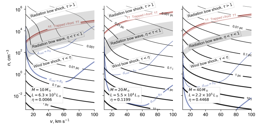
Figure 2: Bow shell regimes in parameter space ($v,n$) of the external stream for main-sequence OB stars of different masses: (a) $10\text{\,}\mathrm{M}_{\odot}$, (b) $20\text{\,}\mathrm{M}_{\odot}$, (c) $40\text{\,}\mathrm{M}_{\odot}$. In all cases, $\kappa=$600\text{\,}\mathrm{c}\mathrm{m}^{2}\,\mathrm{g}^{-1}$$ and efficient gas-grain coupling is assumed. Solid black lines of varying thickness show the bow shell size (star-apex separation, $R_{0}$), while gray shading shows the radiation bow wave regime, with lower border $\tau=\eta_{\text{w}}$ and upper border $\tau=1$, where $\tau=2\kappa\rho R_{0}$ is the optical depth through the bow. For bow shells above the red solid line, the ionization front is trapped inside the bow shell (§ 3.1). Blue lines delineate different cooling regimes (§ 3.2). Above the thin blue line ($d_{\text{cool}}=h_{0}$), the bow shock radiates efficiently, forming a thin shocked shell. Below the thick blue line ($d_{\text{cool}}=R_{0}$), the bow shock is essentially non-radiative.

We consider the canonical case of a bow shell around a star of bolometric luminosity, $L$, with a radiatively driven wind, which is immersed in an external stream of gas and dust with density, $\rho$, and velocity, $v$. The size and shape of the bow shell is determined by a generalized balance of pressure (or, equivalently, momentum) between internal and external sources. We assume that the stream is supersonic and super-alfvenic, so that the external pressure is dominated by the ram pressure, $\rho v^{2}$, and that dust grains and gas are perfectly coupled by collisions (the breakdown of this assumption is the topic of Paper II).

Although dust grains typically constitute only a small fraction $Z_{\text{d}}\sim 0.01$ of the mass of the external stream, they nevertheless dominate the broad-band opacity at FUV, optical and IR wavelengths if they are present. They also dominate at EUV wavelengths ($\lambda<$912\text{\,}\mathrm{\SIUnitSymbolAngstrom}$$), if the hydrogen neutral fraction is less than $\approx 0.001$. The strong coupling assumption means that all the radiative forces applied to the dust grains are directly felt by the gas also.

2.1 Bow shells supported by radiation and wind

The internal pressure is the sum of wind ram pressure and the effective radiation pressure that acts on the bow shell. The radiative momentum loss rate of the star is $L/c$ and the wind momentum loss rate can be expressed as

$$\dot{M}V=\eta_{\text{w}}L/c\ ,$$ (1)

where $\eta_{\text{w}}$ is the momentum efficiency of the wind, which is $<1$ in all cases except WR stars (Lamers & Cassinelli, 1999). If the optical depth at UV/optical wavelengths is sufficiently large, then all of the stellar radiative momentum, emitted with rate $L/c$, is trapped by the bow shell. At the infrared wavelengths where the absorbed radiation is re-emitted, the grain opacity is much lower, so the bow shell is optically thin to this radiation. Combined with the fact that the UV single-scattering albedo is only $\approx 0.5$, this means that the single-scattering limit is approximately valid, and we adopt it here.

We define a fiducial bow shock radius $R_{*}$ in the optically thick, radiation-only limit by balancing stellar radiation pressure against stream ram pressure at the bow apex along the symmetry axis from the star:

$$\frac{L}{4\pi cR_{*}^{2}}=\rho v^{2}\ ,$$ (2)

which yields

$$R_{*}=\left(\frac{L}{4\pi c\rho v^{2}}\right)^{1/2}\ .$$ (3)

We now consider the opposite, optically thin limit. If the total opacity (gas plus dust) per total mass (gas plus dust) is $\kappa$ (with units of $\mathrm{c}\mathrm{m}^{2}\,\mathrm{g}^{-1}$), then the radiative acceleration is

$$a_{\text{rad}}=\frac{\kappa L}{4\pi cR^{2}}\ .$$ (4)

Therefore, an incoming stream with initial velocity, $v_{\infty}$, can be brought to rest by radiation alone at a distance $R_{**}$ where

$$\int_{R_{**}}^{\infty}a_{\text{rad}}\,dr=\tfrac{1}{2}v_{\infty}^{2}\ ,$$ (5)

yielding

$$R_{**}=\frac{\kappa L}{2\pi cv_{\infty}^{2}}\ .$$ (6)

On the other hand, we can also argue as in the optically thick case above by approximating the bow shell as a surface, and balancing stellar radiation pressure against the ram pressure of the incoming stream. The important difference when the shell is not optically thick is that only a fraction $1-e^{-\tau}$ of the radiative momentum is absorbed by the bow, so that equation (2) is replaced with

$$\frac{L(1-e^{-\tau})}{4\pi cR_{0}^{2}}=\rho v^{2}\ .$$ (7)

In the optically thin limit, $1-e^{-\tau}\approx\tau$, so these two descriptions can be seen to agree ($R_{0}\to R_{**}$) so long as

$$\tau=2\kappa\rho R_{0}\ ,$$ (8)

which we will assume to hold generally.

We define a fiducial optical depth,

$$\tau_{*}=\rho\kappa R_{*}\ .$$ (9)

With these fiducial values established, we return to the combined radiation plus wind scenario. Adding the stellar wind ram pressure term from equation (1) allows us to write the general bow shell radius in terms of the fiducial radius as

$$R_{0}=xR_{*}\ ,$$ (10)

where $x$ is the solution of

$$x^{2}-\bigl{(}1-e^{-2\tau_{*}x}\bigr{)}-\eta_{\text{w}}=0\ .$$ (11)

Since this is a transcendental equation, $x$ must be found numerically, but we can write explicit expressions for three limiting cases:

$$x\approx\begin{cases}\text{if $\tau_{*}\gg 1$:}&(1+\eta_{\text{w}})^{1/2}\\ \text{if $\tau_{*}^{2}\ll 1$:}&\tau_{*}+\bigl{(}\tau_{*}^{2}+\eta_{\text{w}}\bigr{)}^{1/2}\approx\begin{cases}\text{if $\tau_{*}^{2}\gg\eta_{\text{w}}$:}&2\tau_{*}\\ \text{if $\tau_{*}^{2}\ll\eta_{\text{w}}$:}&\eta_{\text{w}}^{1/2}\end{cases}\end{cases}$$ (12)

The first case, $x\approx(1+\eta_{\text{w}})^{1/2}$, corresponds to a radiation bow shock (RBS); the second case, $x\approx 2\tau_{*}$, corresponds to a radiation bow wave (RBW); and the third case, $x\approx\eta_{\text{w}}^{1/2}$, corresponds to a wind bow shock (WBS). The two bow shock cases are similar in that the external stream is oblivious to the presence of the star until it suddenly hits the bow shock shell, differing only in whether it is radiation or wind that is providing the internal pressure. In the intermediate bow wave case, on the other hand, the external stream is gradually decelerated by absorption of photons as it approaches the bow. We remark that a shock can still form in this case, but shocked material constitutes only a fraction of the total column density of the shell, as we will show in § 3.3.

2.2 Dependence on stellar type

Table 1: Stellar parameters for example stars

	$M/$\mathrm{M}_{\odot}$$	$L_{4}$	$\dot{M}_{-7}$	$V_{3}$	$\eta_{\text{w}}$	Sp. Type	$T_{\text{eff}}/$\mathrm{k}\mathrm{K}$$	$\lambda_{\text{eff}}$ / $\mathrm{\SIUnitSymbolMicro m}$	$S_{49}$	Figures
	$10$	$0.63$	$0.0034$	$2.47$	$0.0066$	B1.5 V	$25.2$	$0.115$	$0.000\,13$	2a
Main-sequence OB stars	$20$	$5.45$	$0.492$	$2.66$	$0.1199$	O9 V	$33.9$	$0.086$	$0.16$	2b, 8
	$40$	$22.2$	$5.1$	$3.31$	$0.4468$	O5 V	$42.5$	$0.068$	$1.41$	2c
Blue supergiant star	$33$	$30.2$	$20.2$	$0.93$	$0.3079$	B0.7 Ia	$23.5$	$0.123$	$0.016$	4
Red supergiant star	$20$	$15.6$	$100$	$0.015$	$0.0476$	M1 Ia	$3.6$	$0.805$	$0$	3

We now consider the application to bow shocks around main sequence OB stars, as well as cool and hot supergiants, expressing stellar and ambient parameters in terms of typical values as follows:

$$\dot{M}_{-7} =\dot{M}/\bigl{(}${10}^{-7}\text{\,}\mathrm{M}_{\odot}\,\mathrm{y}\mathrm{r}^{-1}$\bigr{)}$$

$$V_{3} =V/\bigl{(}$1000\text{\,}\mathrm{k}\mathrm{m}\,\mathrm{s}^{-1}$\bigr{)}$$

$$L_{4} =L/\bigl{(}${10}^{4}\text{\,}\mathrm{L}_{\odot}$\bigr{)}$$

$$v_{10} =v_{\infty}/\bigl{(}$10\text{\,}\mathrm{k}\mathrm{m}\,\mathrm{s}^{-1}$\bigr{)}$$

$$n =(\rho/\bar{m})/\bigl{(}$1\text{\,}\mathrm{c}\mathrm{m}^{-3}$\bigr{)}$$

$$\kappa_{600} =\kappa/\bigl{(}$600\text{\,}\mathrm{c}\mathrm{m}^{2}\,\mathrm{g}^{-1}$\bigr{)}\ ,$$

where $\bar{m}$ is the mean mass per hydrogen nucleon ($\bar{m}\approx 1.3m_{\text{p}}\approx$2.17\text{\times}{10}^{-24}\text{\,}\mathrm{g}$$ for solar abundances). Note that $\kappa=$600\text{\,}\mathrm{c}\mathrm{m}^{2}\,\mathrm{g}^{-1}$$ corresponds to a cross section of $\approx${10}^{-21}\text{\,}\mathrm{c}\mathrm{m}^{2}$$ per hydrogen nucleon, which is typical for interstellar medium dust (Bertoldi & Draine, 1996) at far ultraviolet wavelengths, where OB stars emit most of their radiation. In terms of these parameters, we can express the stellar wind momentum efficiency as

$$\eta_{\text{w}}=$0.495$\,\dot{M}_{-7}\,V_{3}\,L_{4}^{-1}$$ (13)

and the fiducial radius and optical depth as

$$R_{*}/$\mathrm{p}\mathrm{c}$ =$2.21$\,(L_{4}/n)^{1/2}\,v_{10}^{-1}$$ (14)

$$\tau_{*} =$0.0089$\,\kappa_{600}\,(L_{4}\,n)^{1/2}\,v_{10}^{-1}\ .$$ (15)

In Figure 2, we show results for the bow size (apex distance, $R_{0}$) as a function of the density, $n$, and relative velocity, $v_{\infty}$, of the external stream, with each panel corresponding to a particular star, with parameters as shown in Table 1. To facilitate comparison with previous work, we choose stellar parameters similar to those used in the hydrodynamical simulations of Meyer et al. (2014, 2016, 2017), based on stellar evolution tracks for stars of $10\text{\,}\mathrm{M}_{\odot}20\text{\,}\mathrm{M}_{\odot}40\text{\,}\mathrm{M}_{\odot}$ (Brott et al., 2011) and theoretical wind prescriptions (de Jager et al., 1988; Vink et al., 2000). Although the stellar parameters do evolve with time, they change relatively little during the main-sequence lifetime of several million years. The three examples are an early B star ($10\text{\,}\mathrm{M}_{\odot}$), a late O star ($20\text{\,}\mathrm{M}_{\odot}$), and an early O star ($40\text{\,}\mathrm{M}_{\odot}$), which cover the range of luminosities and wind strengths expected from bow-producing hot main sequence stars. The luminosity is a steep function of stellar mass ($L\sim M^{2.5}$) and the wind mass-loss rate is a steep function of luminosity ($\dot{M}\sim L^{2.2}$), which means that the wind momentum efficiency is also a steep function of mass ($\eta_{\text{w}}\sim M^{3}$), approaching unity for early O stars, but falling to less than 1% for B stars.

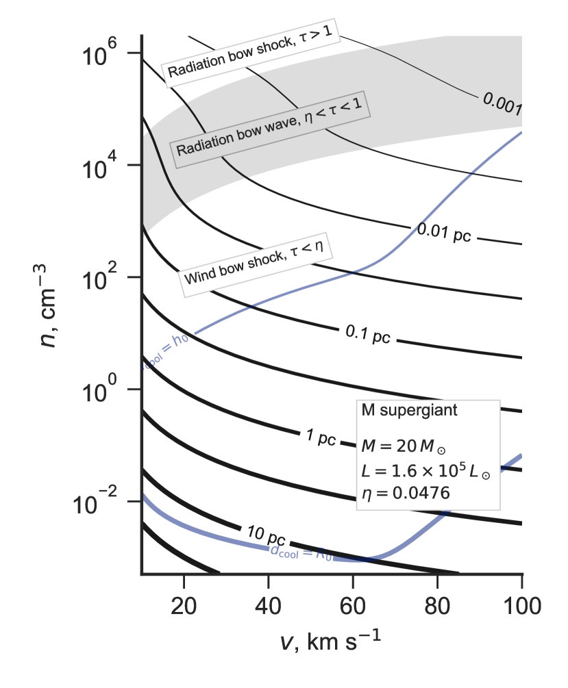
Figure 3: As Fig. 2, but for a cool M-type supergiant instead of hot main sequence stars. A smaller dust opacity is used, $\kappa=$60\text{\,}\mathrm{c}\mathrm{m}^{2}\,\mathrm{g}^{-1}$$, because of the reduced extinction efficiency at the optical/infrared wavelengths emitted by this star.

It can be seen from Figure 2 that the onset of the radiation bow wave regime is very similar for the three main-sequence stars, occurring at $n>\text{$2040$}\,v_{10}^{2}$. An important difference, however, is that for the $40\text{\,}\mathrm{M}_{\odot}$ star, which has a powerful wind, the radiation bow wave regime only occurs for a very narrow range of densities, whereas for the $10\text{\,}\mathrm{M}_{\odot}$ star, with a much weaker wind, the regime is much broader, extending to $n<${10}^{4}$\,v_{10}^{2}$. Another difference is the size scale of the bow shells in this regime, which is $R_{0}=\text{$0.001\text{\,}\mathrm{p}\mathrm{c}0.003\text{\,}\mathrm{p}\mathrm{c}$}$ for the $10\text{\,}\mathrm{M}_{\odot}$ star if $v_{\infty}=$40\text{\,}\mathrm{k}\mathrm{m}\,\mathrm{s}^{-1}$$, but $R_{0}\approx$0.1\text{\,}\mathrm{p}\mathrm{c}$$ for the $40\text{\,}\mathrm{M}_{\odot}$ star, assuming the same inflow velocity.

Figure 3 shows results for a cool M-type super-giant star with stellar parameters inspired by Betelgeuse ( Orionis), as listed in Table 1. Unlike the UV-dominated spectrum of the hot stars, this star emits predominantly in the near-infrared, where the dust extinction efficiency is lower (Weingartner & Draine, 2001), so we adopt a lower opacity of $60\text{\,}\mathrm{c}\mathrm{m}^{2}\,\mathrm{g}^{-1}$. This has the effect of shifting the radiation bow wave regime to higher densities: $n=\text{$100030\,000$}\,v_{10}^{2}$ in this case.

2.3 Effects of stellar gravity

In principle, gravitational attraction from the star, of mass $M$, will partially counteract the radiative acceleration. This can be accounted for by replacing $L$ with an effective luminosity

$$L_{\text{eff}}=L\bigl{(}1-\Gamma_{\text{E}}^{\,-1}\bigr{)}\ ,$$ (16)

in which $\Gamma_{\text{E}}$ is the Eddington factor:

$$\Gamma_{\text{E}}=\frac{\kappa L}{4\pi cGM}=458.5\,\frac{\kappa_{600}L_{4}}{M}\ ,$$ (17)

where, in the last expression, $M$ is measured in solar masses. For the stars in Table 1, we find $\Gamma_{\text{E}}\approx\text{$30400$}$, so gravity can be safely ignored. When the optical depth of the bow shell is very large, $\tau>\ln\Gamma_{\text{E}}\sim 5$, gravity will exceed the radiation force in the outer parts of the shell (see Rodríguez-Ramírez & Raga 2016), but it is generally too weak to affect the shell structure even in such a case, see § 3.3 below.

3 Physical state of the bow shell

There are two shocked zones in the bow: an inner zone of shocked stellar wind, and an outer zone of decelerated ambient stream. For OB stars, dust grains are present only in the ambient stream, whereas for cool stars they will also be present in the stellar wind. In the remainder of this paper, we will concentrate on the OB star case, where it is the outer zone that is most important observationally. Bow shells are typically detected via their infrared radiation (absorption and re-emission by dust of stellar radiation), or by emission lines such as the hydrogen H$\alpha$ line.

3.1 Ionization state

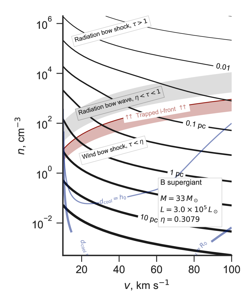
Figure 4: As Fig. 2, but for an evolved B-type supergiant instead of main sequence stars. This is similar to the early O MS star of Fig. 2c in many respects, except for the trapping of the ionization front, which occurs for much lower outer stream densities.

In this section we calculate whether the star is capable of photoionizing the entire bow shock shell, or whether the ionization front will be trapped within it. Using the on-the-spot approximation for the diffuse fields (Osterbrock & Ferland, 2006), the number of hydrogen recombinations per unit time per unit area in a fully ionized shell of density $n_{\text{sh}}$ and thickness $h_{\text{sh}}$ is

$$\mathcal{R}=\alpha_{\text{B}}n_{\text{sh}}^{2}h_{\text{sh}}\ ,$$ (18)

where $\alpha_{\text{B}}=$2.6\text{\times}{10}^{-13}$\,T_{4}^{-0.7}\,$\mathrm{c}\mathrm{m}^{3}\,\mathrm{s}^{-1}$$ is the case B recombination coefficient and $T_{4}=T/${10}^{4}\text{\,}\mathrm{K}$$. The advective flux of hydrogen nuclei through the shock is

$$\mathcal{A}=nv_{\infty}\ ,$$ (19)

and the flux of hydrogen-ionizing photons ($h\nu>$13.6\text{\,}\mathrm{e}\mathrm{V}$$) incident on the inner edge of the shell is

$$\mathcal{F}=\frac{S}{4\pi R_{0}^{2}}\ ,$$ (20)

where $S$ is the ionizing photon luminosity of the star. Any shell with $\mathcal{R}+\mathcal{A}>\mathcal{F}$ cannot be entirely photoionized by the star, and so must have trapped the ionization front.

The ratio of advective particle flux to ionizing flux is, from equations (3), (19), (20),

$$\frac{\mathcal{A}}{\mathcal{F}}=$5.86\text{\times}{10}^{-5}$\frac{x^{2}L_{4}}{v_{10}S_{49}}\ ,$$ (21)

where

$$S_{49}=S/\bigl{(}${10}^{49}\text{\,}\mathrm{s}^{-1}$\bigr{)}\ .$$

Numerical values of $S_{49}$ for our three example stars are given in Table 1, taken from Figure 4 of Sternberg et al. (2003). Since $\mathcal{A}\ll\mathcal{F}$ in nearly all cases, for clarity of exposition we ignore $\mathcal{A}$ in the following discussion, although it is included in quantitative calculations. The column density of the shocked shell can be found, for example, from equations (10) and (12) of Wilkin (1996) in the limit $v_{\infty}/V\to 0$ (Wilkin’s parameter $\alpha$) and $\theta\to 0$. This yields

$$n_{\text{sh}}h_{\text{sh}}=\tfrac{3}{4}nR_{0}\ .$$ (22)

Assuming strong cooling behind the shock (§ 3.2), the shell density is

$$n_{\text{sh}}=\mathcal{M}_{0}^{2}n\,$$ (23)

where $\mathcal{M}_{0}=v_{\infty}/c_{\text{s}}$ is the isothermal Mach number of the external stream. Putting these together with equations (3) and  (9), one finds that $\mathcal{R}>\mathcal{F}$ implies

$$x^{3}\tau_{*}>\frac{4Scc_{\text{s}}^{2}\bar{m}^{2}\kappa}{3\alpha L}\ .$$ (24)

From equation (11), it can be seen that $x$ depends on the external stream parameters, $n$, $v_{\infty}$ only via $\tau_{*}$, and so equation (24) is a condition for $\tau_{*}$, which, by using equation (15), becomes a condition on $n/v_{10}^{2}$. In the radiation bow shock case, $x=(1+\eta_{\text{w}})^{1/2}$, and the condition can be written:

$$\text{RBS:}\quad\frac{n}{v_{10}^{2}}>$2.65\text{\times}{10}^{8}$\,\frac{S_{49}^{2}T_{4}^{3.4}}{L_{4}^{3}(1+\eta_{\text{w}})^{3}}\ .$$ (25)

In the radiation bow wave case, $x=2\tau_{*}$, and the condition can be written:

$$\text{RBW:}\quad\frac{n}{v_{10}^{2}}>$5.36\text{\times}{10}^{4}$\,\frac{S_{49}^{1/2}T_{4}^{0.85}}{\kappa_{600}^{3/2}L_{4}^{3/2}}\ .$$ (26)

In the wind bow shock case, the result is the same as equation (25), but changing the factor $(1+\eta_{\text{w}})^{3}$ to $\eta_{\text{w}}^{3}$. For the example hot stars in Table 1, and assuming $\kappa_{600}=1$, $T_{4}=0.8$, the resulting density threshold is $n>(\text{$10005000$})\,v_{10}^{2}$, depending only weakly on the stellar parameters, which is shown by the red lines in Figure 2. For the $10\text{\,}\mathrm{M}_{\odot}$ star this is in the radiation bow wave regime, whereas for the higher mass stars it is in the radiation bow shock regime. When the external stream is denser than this, then the outer parts of the shocked shell may be neutral instead of ionized, giving rise to a cometary compact H ii region (Mac Low et al., 1991; Arthur & Hoare, 2006). This is only necessarily true, however, when the star is isolated. If the star is in a cluster environment, then the contribution of other nearby massive stars to the ionizing radiation field must be considered.

Quite different results are obtained for a B-type supergiant star (see Tab. 1 and Fig. 4), which has a similar bolometric luminosity and wind strength to the $40\text{\,}\mathrm{M}_{\odot}$ main-sequence star, but a hundred times lower ionizing luminosity. This results in a far lower threshold for trapping the ionization front of $n>40v_{10}^{2}$. The advective flux, $\mathcal{A}$, is relatively stronger for this star than for the main-sequence stars, but even for $v_{10}<2$, where the effect is strongest, the change is only of order the thickness of the dark red line in Figure 4.

In principle, when the ionization front trapping occurs in the bow wave regime, then the curves for $R_{0}$ will be modified in the region above the red line because all of the ionizing radiation is trapped in the shell due to gas opacity, which is not included in equation (8). However, this only happens for our $10\text{\,}\mathrm{M}_{\odot}$ star, which has a relatively soft spectrum. Table 1 gives the peak wavelength of the stellar spectrum for this star as $\lambda_{\text{eff}}=$0.115\text{\,}\mathrm{\SIUnitSymbolMicro m}$$, which is significantly larger than the hydrogen ionization threshold at $0.0912\text{\,}\mathrm{\SIUnitSymbolMicro m}$, meaning that only a small fraction of the total stellar luminosity is in the EUV band and affected by the gas opacity. The effect on $R_{0}$ is therefore small. For the higher mass stars, $\lambda_{\text{eff}}<$0.0912\text{\,}\mathrm{\SIUnitSymbolMicro m}$$, so the majority of the luminosity is in the EUV band, but in these cases the ionization front trapping occurs well inside the radiation bow shock zone, where the dust optical depth is already sufficient to trap all of the radiative momentum.

3.2 Efficiency of radiative cooling

In this section, we calculate whether the radiative cooling is sufficiently rapid behind the bow shock to allow the formation of a thin, dense shell. In general, cooling is least efficient at low densities, so we will assume that the wind bow shock regime applies unless otherwise specified. We label quantities just outside the shock by the subscript “0”, quantities just inside the shock (after thermalization, but before any radiative cooling) by the subscript “1”, and quantities after the gas has cooled back to the photoionization equilibrium temperature by the subscript “2”. Assuming a ratio of specific heats, $\gamma=5/3$, the relation between the pre-shock and immediate post-shock quantities (Zel’Dovich & Raizer, 1967) is

$$\frac{n_{1}}{n_{0}} =\frac{4\mathcal{M}_{0}^{2}}{\mathcal{M}_{0}^{2}+3}$$ (27)

$$\frac{T_{1}}{T_{0}} =\tfrac{1}{16}\bigl{(}5\mathcal{M}_{0}^{2}-1\bigr{)}\bigl{(}1+3/\mathcal{M}_{0}^{2}\bigr{)}$$ (28)

$$\frac{v_{1}}{v_{0}} =\left(\frac{n_{1}}{n_{0}}\right)^{-1}\ ,$$ (29)

where $\mathcal{M}_{0}=v_{0}/c_{\text{s}}$. The cooling length of the post-shock gas can be written as

$$d_{\text{cool}}=\frac{3P_{1}v_{1}}{2\bigl{(}\mathcal{L}_{1}-\mathcal{G}_{1}\bigr{)}}\ ,$$ (30)

where $P_{1}$ is the thermal pressure and $\mathcal{L}_{1}$, $\mathcal{G}_{1}$ are the volumetric radiative cooling and heating rates. For fully photoionized gas, we have $P_{1}\approx 2n_{1}kT_{1}$, $\mathcal{L}_{1}=n_{1}^{2}\Lambda(T_{1})$, and $\mathcal{G}_{1}=n_{1}^{2}\Gamma(T_{1})$, where $\Lambda(T)$ is the cooling coefficient, which is dominated by metal emission lines that are excited by electron collisions, and $\Gamma(T)$ is the heating coefficient, which is dominated by hydrogen photo-electrons (Osterbrock & Ferland, 2006). The cooling coefficient has a maximum around ${10}^{5}\text{\,}\mathrm{K}$, and for typical ISM abundances can be approximated as follows:

$$\Lambda_{\text{warm}} =$3.3\text{\times}{10}^{-24}$\,T_{4}^{2.3}\,$\mathrm{e}\mathrm{r}\mathrm{g}\,\mathrm{c}\mathrm{m}^{3}\,\mathrm{s}^{-1}$$$ (31)

$$\Lambda_{\text{hot}} =${10}^{-20}$\,T_{4}^{-1}\,$\mathrm{e}\mathrm{r}\mathrm{g}\,\mathrm{c}\mathrm{m}^{3}\,\mathrm{s}^{-1}$$$ (32)

$$\Lambda =\left(\Lambda_{\text{warm}}^{-k}+\Lambda_{\text{hot}}^{-k}\right)^{-1/k}\quad\text{with}\quad k=3\ ,$$ (33)

which is valid in the range $0.7<T_{4}<1000$. We approximate the heating coefficient as

$$\Gamma=$1.77\text{\times}{10}^{-24}$\,T_{4}^{-1/2}\,$\mathrm{e}\mathrm{r}\mathrm{g}\,\mathrm{c}\mathrm{m}^{3}\,\mathrm{s}^{-1}$\ ,$$ (34)

where the coefficient is chosen so as to give $\Gamma=\Lambda$ at an equilibrium temperature of $T_{4}=0.8$.

In Figure 2 we show curves calculated from equations (27) to (34), corresponding to $d_{\text{cool}}=R_{0}$ (thick blue line) and $d_{\text{cool}}=h_{0}$ (thin blue line), where $h_{0}$ is the shell thickness in the limit of instantaneous cooling. In this context, $n_{0}=n$ and $n_{2}=n_{\text{sh}}$, so that $h_{0}$ follows from equations (22) and (23) as

$$h_{0}=\tfrac{3}{4}\mathcal{M}_{0}^{-2}R_{0}\ .$$ (35)

The bends in the curves at $v\approx$50\text{\,}\mathrm{k}\mathrm{m}\,\mathrm{s}^{-1}$$ are due to the maximum in the cooling coefficient $\Lambda(T)$ around ${10}^{5}\text{\,}\mathrm{K}$. For bow shells with outer stream densities above the thin blue line, radiative cooling is so efficient that the bow shock can be considered isothermal, and so the shell is dense and thin (at least, in the apex region). It can be seen that the ionization front trapping always occurs at densities larger than this, which justifies the use of equation (23) in the previous section. For bow shells with outer stream densities below the thick blue line, cooling is unimportant and the bow shock can be considered non-radiative. In this case the shell is thicker than in the radiative case, $h_{\text{sh}}/R_{0}\approx\text{$0.20.3$}$. This value can be found from equation (22) by substituting $n=n_{0}$ and $n_{\text{sh}}\approx 1.1n_{1}$, then using equation (27). The factor $1.1$ comes from consideration of the slight increase in density between the shock and the contact/tangential discontinuity. For bow shells with outer stream densities between the two blue lines, cooling does occur, albeit inefficiently, so that the shell thickness $h_{\text{sh}}$ is set by $d_{\text{cool}}$ rather than $h_{0}$.

3.3 Axial structure of bow shells

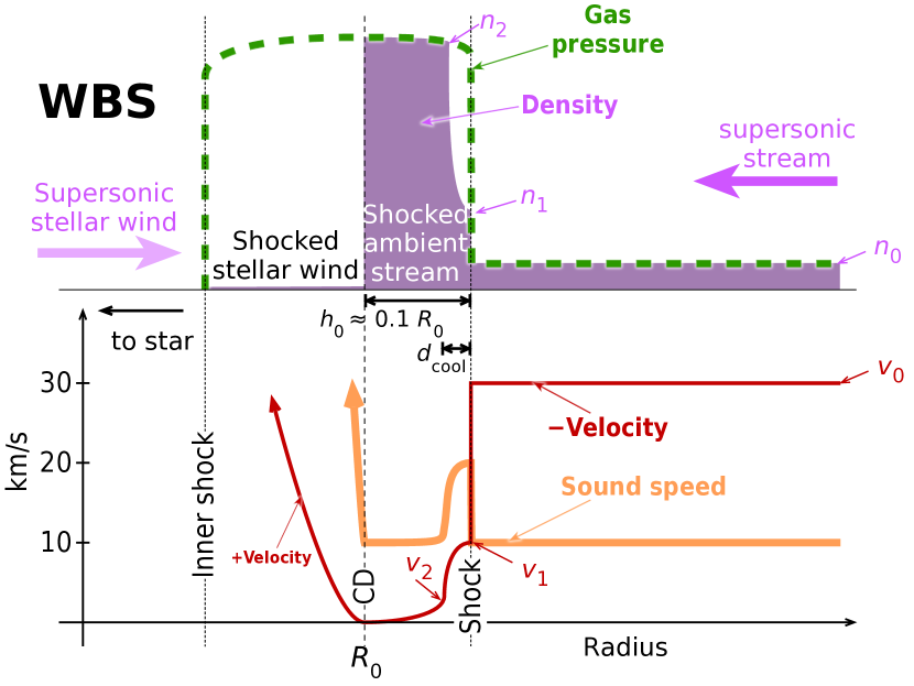
Figure 5: Profiles of physical variables along the axis of the bow shell for a wind-supported bow shock. The top panel shows the gas density (purple) and the gas thermal pressure (green dashed line) as a function of radius from the star. The bottom panel shows the absolute value of the gas velocity (red line) and sound speed (orange line). The stellar wind comes from the left with positive velocity, while the ambient stream comes from the right. All velocities are in the frame of reference of the star, which is located off the left-hand edge of the figure. The case shown is for a stream velocity of $30\text{\,}\mathrm{k}\mathrm{m}\,\mathrm{s}^{-1}$ and an equilibrium ionized sound speed of $10\text{\,}\mathrm{k}\mathrm{m}\,\mathrm{s}^{-1}$, with a post-shock cooling length $d_{\text{cool}}$ that is smaller than the shell thickness $h_{0}$. The different flow regions are described in the text.

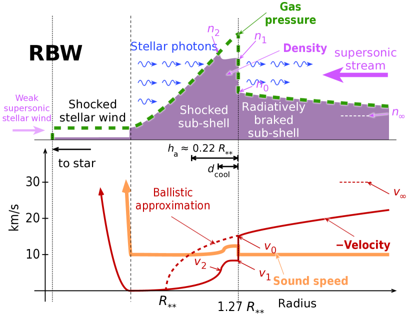
Figure 6: As Fig. 5 but for a radiation-supported bow wave. The heavy dashed red line in the lower panel shows the ballistic approximation to the velocity profile, which would be followed in the case of a highly supersonic incident stream. The ambient stream is gradually decelerated by absorption of stellar radiation, leading to a lower velocity and higher density just before the shock, $v_{0}$ and $n_{0}$, as compared to the values at large distances, $v_{\infty}$ and $n_{\infty}$, which are shown by dashed horizontal lines.

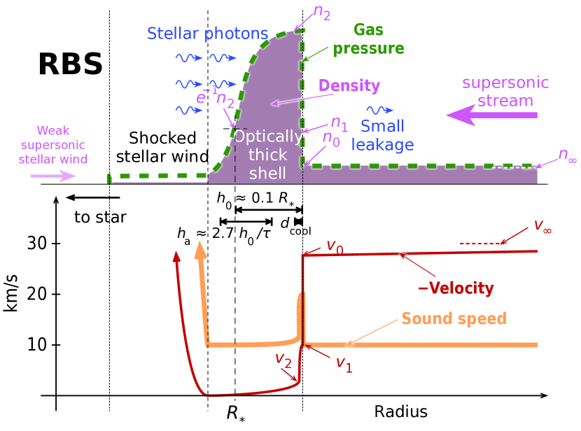
Figure 7: As Fig. 5 but for a radiation-supported bow shock. A smaller cooling length is assumed than in the previous figures since the RBS regime occurs at higher ambient densities.

In the shell of a wind-supported bow shock, the gas density is highest at the contact discontinuity, but this is no longer true for radiation-supported bow shells, as illustrated in Figures 5 to 7, where we schematically show the shell structure for the three cases: WBS, RBW, and RBS. In all cases, we assume a far-field mach number of $\mathcal{M}_{\infty}=3$ for the incident stream of density $n_{\infty}$. For the WBS case (Fig. 5), the stream is unchanged until it reaches the shock, so $\mathcal{M}_{0}=\mathcal{M}_{\infty}$ and $n_{0}=n_{\infty}$. The density increases to $n_{1}=3n_{0}$ in the shock (eq. [27]), and then to $n_{2}=9n_{0}$ (eq. [23]) after it has cooled back down to the equilibrium photoionized temperature. In the figure, we show the case where $d_{\text{cool}}<h_{0}$, so that most of the shell is at roughly constant density. Note that although the mass flux along the axis, $nv$, is approximately conserved in most of the flow, this is no longer true close to the contact discontinuity, since the streamlines bend away from the axis due to lateral pressure gradients. This is what allows $v$ to tend to zero, while $n$ remains constant. The thermal pressure in the shocked stellar wind is equal to the shell pressure, but its density is much smaller due to a temperature that is higher by a factor of $\approx 3100V_{3}^{2}$, (eq. [28], assuming inefficient cooling).

For the optically thin RBW case (Fig. 6), equations (4) to (6) can be combined to give the radial dependence of the stream velocity as it approaches the star:

$$v(R)=\left(1-\frac{R_{**}}{R}\right)^{1/2}v_{\infty}\ .$$ (36)

This ballistic approximation (shown by the dashed red line in Fig. 6) predicts that the velocity smoothly decreases to zero at $R=R_{**}$. However, although this is valid in the limit of high Mach number, it ignores the effects of gas pressure and so becomes invalid once the stream velocity falls close to the sound speed. The situation bears similarities to the flow in a supersonic diffuser, such as the inlet of a ramjet or other supersonic aircraft engine (Seddon & Goldsmith, 1999), which slows supersonic airflow down to subsonic speeds before combustion. Exactly the opposite flow configuration is present in a rocket nozzle (Courant & Friedrichs, 1948), where the flow can smoothly pass from subsonic to supersonic velocities at the throat of the nozzle. An analogy between an isothermal stellar wind and a rocket nozzle is developed in detail in § 3.5 of Lamers & Cassinelli (1999). However, in the reverse case of a supersonic diffuser, a smooth transition from supersonic to subsonic flow is not possible (Morawetz, 1956). Instead, a normal shock wave develops, which decelerates the supersonically entering flow, allowing it to exit subsonically (Embid et al., 1984; Hafez & Guo, 1999). The supersonic inlet/bow wave analogy is not so exact as the rocket nozzle/stellar wind analogy due to the multi-dimensional nature of the bow shell, which means that lateral flows of gas away from the apex become important when the velocity is subsonic. Nonetheless, we expect that a normal shock must be present in the flow, although there does not seem to be any simple argument for predicting the exact Mach number where it will occur. In Figure. 6 we assume that the shock occurs at a Mach number $\mathcal{M}_{0}=1.5$, but multidimensional numerical simulations are necessary to test this supposition.

The shell in the RBW case therefore consists of two parts: an outer radiatively braked sub-shell, and an inner shocked sub-shell. In the outer sub-shell, the density gradually increases inwards as the stream is decelerated by the absorbed photons, reaching

$$n_{0}=\frac{\mathcal{M}_{\infty}}{\mathcal{M}_{0}}n_{\infty}$$ (37)

just outside the shock ($n_{0}=2n_{\infty}$ for the case illustrated). In the inner sub-shell, on the other hand, the pressure must increase outwards, since it is subsonic and therefore in approximate hydrostatic equilibrium with an outward-pointing effective gravity from the radiation force. The shell thickness will be set by the hydrostatic scale height, $h_{a}=c_{\text{s}}^{2}/a_{\text{rad}}$, which by eqs. (4, 6) is given by

$$h_{a}=\frac{2R_{**}}{\mathcal{M}_{\infty}^{2}}\ .$$ (38)

If the cooling is efficient ($d_{\text{cool}}<h_{a}$), then most of the sub-shell is isothermal and the density will fall off exponentially towards the star. The contact discontinuity with the stellar wind will form at the point where the shell pressure has fallen by a factor of order $\tau/\eta_{\text{w}}$, but this has no influence on the bulk of the shell, which is pressurized by radiation, not wind. If, as we suspect, $\mathcal{M}_{0}$ depends only weakly, if at all, on $\mathcal{M}_{\infty}$, then eqs. (37, 38) imply that the inner shocked sub-shell represents a fraction $\approx\mathcal{M}_{\infty}^{-1}$ of the total shell optical depth, which means that the outer supersonic sub-shell dominates for highly supersonic stream velocities.

For the optically thick RBS case (Fig. 7), the shell density profile is no longer simply exponential since the pressure scale height now increases as one moves away from the star, due to the extinction-induced decline in radiation flux. Assuming single scattering and plane geometry, the resultant hydrostatic density profile is doubly exponential:

$$n(R)=n_{2}e^{-e^{-x}}\text{\quad where\quad}x=n_{2}\bar{m}\kappa(R-R_{*})\ .$$ (39)

The shell density increases from $e^{-1}n_{2}$ at $R_{*}$ to saturate at $n_{2}$ for $R>R_{*}+h_{a}$, where $h_{a}$ is now the pressure scale height at the inner edge of the shell. From equations (3, 6, 8, 35, 38), and taking $R_{0}\approx R_{*}$, we find

$$h_{a}\approx\frac{4h_{0}}{3\tau}\ .$$ (40)

We show results for a total shell optical depth $\tau=3$, for which $h_{a}$ is a significant fraction of $h_{0}$. For much larger optical depths, $h_{0}\gg h_{a}$ so that the constant density portion of the shell will dominate the total column. A small fraction $e^{-\tau}$ of the photons will penetrate the shell and be available to decelerate the supersonic stream, as in the RBW case, yielding $v_{0}=(1-\tau e^{-\tau})\,v_{\infty}$. In the illustrated case of $\tau=3$, the resultant speed reduction before the shock is only 8%. As mentioned in § 2.3, radiative acceleration becomes less important than gravity in the outer regions of an opaque shell. However, in order for this to have a significant effect on the shell, the gravitational scale height would have to be be less than the shell thickness: $\Gamma_{\text{E}}h_{a}<h_{0}$. From equation (40) this translates to $\tau>\frac{4}{3}\Gamma_{\text{E}}$, where dust-opacity Eddington factors are $\Gamma_{\text{E}}\sim 100$ for OB stars. Such large optical depths would require extremely high ambient densities of $n>$2\text{\times}{10}^{7}$L_{4}\,v_{10}^{2}\left($10\text{\,}\mathrm{M}_{\odot}$/M\right)^{2}\,$\mathrm{c}\mathrm{m}^{-3}$$, where we have used equations (9, 17) and that $\tau\approx 2\tau_{*}$ in the RBS limit.

4 Discussion

The stellar bow shells modeled in this paper can be seen as either due to the motion of a star through the interstellar medium, or due to the motion of the interstellar medium that flows past the star. The first case corresponds to runaway stars (Blaauw, 1961), which have been ejected from a binary system or stellar cluster (Hoogerwerf et al., 2001), while the second case can be due to photoevaporation and champagne flows in H ii regions (Tenorio-Tagle, 1979; Shu et al., 2002; Henney et al., 2005), or to general turbulent flows in the Galaxy (e.g., Ballesteros-Paredes et al., 1999). In this section, we consider the stream densities and velocities expected in each of these scenarios, and compare them with our predictions for the type of bow shells that should result.

Although some runaway stars have velocities exceeding $100\text{\,}\mathrm{k}\mathrm{m}\,\mathrm{s}^{-1}$, most are moving considerably slower, with a median peculiar velocity of about $30\text{\,}\mathrm{k}\mathrm{m}\,\mathrm{s}^{-1}$ (Tetzlaff et al., 2011). The higher velocity runaways are likely produced by dynamical interactions in the center of young clusters (Gualandris et al., 2004), whereas the supernova-induced dissolution of binary systems is predicted to primarily produce “walkaways” with even slower velocities of order $10\text{\,}\mathrm{k}\mathrm{m}\,\mathrm{s}^{-1}$ (Renzo et al., 2018). Environmental flows are also expected to be of order $10\text{\,}\mathrm{k}\mathrm{m}\,\mathrm{s}^{-1}$, which is a characteristic velocity dispersion for warm neutral gas in the inner Galaxy (Marasco et al., 2017) and also a typical expansion velocity for H i shells (Ehlerová & Palouš, 2005). Internal velocity dispersions within H ii regions are subsonic ($5\text{\,}\mathrm{k}\mathrm{m}\,\mathrm{s}^{-1}10\text{\,}\mathrm{k}\mathrm{m}\,\mathrm{s}^{-1}$) for small regions, such as the Orion Nebula, containing one or a few ionizing stars (Arthur et al., 2016). This increases slowly for more luminous regions as $\sigma\propto L^{1/4}$ (Bordalo & Telles, 2011), so giant star forming complexes such as Carina (100 times more luminous than Orion) show velocity dispersions of order $20\text{\,}\mathrm{k}\mathrm{m}\,\mathrm{s}^{-1}$ (Damiani et al., 2016). Higher velocities of $30\text{\,}\mathrm{k}\mathrm{m}\,\mathrm{s}^{-1}40\text{\,}\mathrm{k}\mathrm{m}\,\mathrm{s}^{-1}$ are reached in divergent photoevaporation flows (Dyson, 1968), but this is achieved at expense of a lower density. Given all the above, we expect there to be many more bow shells with relative stream velocity $v_{\infty}\sim$20\text{\,}\mathrm{k}\mathrm{m}\,\mathrm{s}^{-1}$$ than bow shells with $v_{\infty}\sim$100\text{\,}\mathrm{k}\mathrm{m}\,\mathrm{s}^{-1}$$.

Turning now to the ambient density, if bow shock stars were randomly sampling the volume of the Galactic disk, then we would expect the average density to be $<$1\text{\,}\mathrm{c}\mathrm{m}^{-3}$$. The dominant gas phase (Ferrière, 2001) near the Galactic mid-plane is the Warm Neutral Medium with a volume filling fraction of 45% (Fig. 11 of Kalberla & Kerp, 2009) and an average density of $0.9\text{\,}\mathrm{c}\mathrm{m}^{-3}$ at the Solar circle (§ 4 of Kalberla & Dedes, 2008). Significant fractions of the volume ($\approx 20\%$ each) are also occupied by the Warm Ionized Medium and Hot Ionized Medium, which have even lower densities ($\approx$0.3\text{\,}\mathrm{c}\mathrm{m}^{-3}$$ and ${10}^{-3}\text{\,}\mathrm{c}\mathrm{m}^{-3}$, respectively) and which increasingly dominate the volume for heights $z>$500\text{\,}\mathrm{p}\mathrm{c}$$ above the plane. The denser Cold Neutral Medium ($n\approx\text{$10\text{\,}\mathrm{c}\mathrm{m}^{-3}100\text{\,}\mathrm{c}\mathrm{m}^{-3}$}$) and Molecular Clouds ($n>$1000\text{\,}\mathrm{c}\mathrm{m}^{-3}$$) occupy much smaller volumes ($\approx 10\%$ and $<1\%$, respectively). However, observations of stellar bow shells are clearly biased towards these higher densities.

In part, this bias is due to bow shells being easier to detect in denser environments. Depending on the emission mechanism, the shell luminosity will be proportional to the column density ($\propto nR_{0}$) or volume emission measure ($\propto n^{2}R_{0}^{3}$), which are both increasing functions of $n$ since, from § 2.1, the bow shell size falls relatively slowly as $R_{0}\propto n^{-1/2}$ in the WBS and RBS cases, and is independent of $n$ in the RBW case. Another contribution to the high-density bias is simply that none but the highest velocity high-mass stars can move far during their lifetime from the molecular clouds where they were born. Even a runaway star with $v=$30\text{\,}\mathrm{k}\mathrm{m}\,\mathrm{s}^{-1}$$, will travel $<$120\text{\,}\mathrm{p}\mathrm{c}$$ during an O-star lifetime of $<$4\text{\,}\mathrm{M}\mathrm{y}\mathrm{r}$$, which is of the same order as the sizes of Giant Molecular Clouds. Many observed stellar bow shells are found in high mass star clusters associated with large H ii regions (Povich et al., 2008; Sexton et al., 2015). The ionized gas density in Carina, for example, has an average value of $\approx$100\text{\,}\mathrm{c}\mathrm{m}^{-3}$$ (Oberst et al., 2011; Damiani et al., 2016), although with peaks $>$3000\text{\,}\mathrm{c}\mathrm{m}^{-3}$$ in photoevaporation flows from embedded molecular globules (Smith et al., 2004). In more compact H ii regions, such as the Orion Nebula, ionized densities up to ${10}^{4}\text{\,}\mathrm{c}\mathrm{m}^{-3}$ are found on scales of about $0.1\text{\,}\mathrm{p}\mathrm{c}$ (Weilbacher et al., 2015; O’Dell et al., 2017).

In § 2.2 we found that the bow shell is wind-supported when $\tau_{*}^{2}<\eta_{\text{w}}$, where $\tau_{*}$ is a fiducial optical depth (eq. [15]) and $\eta_{\text{w}}$ is the radiative momentum efficiency of the stellar wind (eq. [13]). This translates into a maximum stream density for wind-supported bow shells of

$$n_{\text{max}}\approx\left($30\text{\,}\mathrm{c}\mathrm{m}^{-3}$\right)\left(\frac{v}{$10\text{\,}\mathrm{k}\mathrm{m}\,\mathrm{s}^{-1}$}\right)^{2}\left(\frac{\eta_{\text{w}}}{\eta_{\text{\tiny Vink}}}\right)\left(\frac{$600\text{\,}\mathrm{c}\mathrm{m}^{2}\,\mathrm{g}^{-1}$}{\kappa}\right)\ ,$$ (41)

which is largely insensitive to spectral type between early-B and early-O stars. In this equation, we have expressed the wind efficiency in terms of the Table 1 values, $\eta_{\text{\tiny Vink}}$, which are calculated from the Vink et al. (2000) recipe, and the UV dust opacity in terms of the standard ISM value adopted in § 2.2.

Therefore, runaway stars moving through the diffuse ISM with $n\sim$1\text{\,}\mathrm{c}\mathrm{m}^{-3}$$ and $v\sim$30\text{\,}\mathrm{k}\mathrm{m}\,\mathrm{s}^{-1}$$ are safely in the WBS regime, having $n\approx$0.004$\,n_{\text{max}}$ for the default wind and dust parameters. On the other hand, slow-moving stars in H ii regions of moderate density ($n\sim$100\text{\,}\mathrm{c}\mathrm{m}^{-3}$$) can easily have $n>n_{\text{max}}$, meaning that their bow shells will be radiation supported.

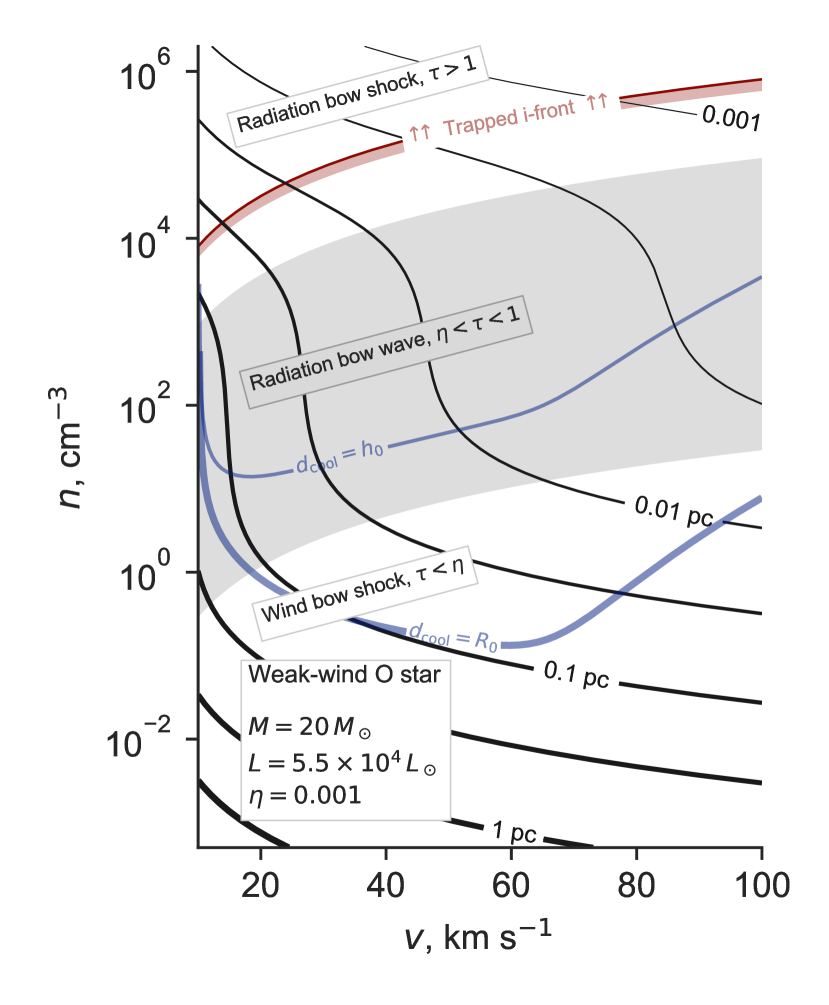
Figure 8: As Fig. 2, but for a weak-wind O star, similar to the sample observed by Martins et al. (2005). For this star, radiation-supported bow waves (gray shading) occur over a much larger region of parameter space than for a normal-wind star of the same spectral type (see Fig. 2b).

For cases where the stellar wind or dust properties differ from our assumed values, then these conclusions may change. For instance, there are a growing number of stars for which very low mass-loss rates have been diagnosed from UV, optical or infrared line profiles (Martins et al., 2005; Marcolino et al., 2009; Najarro et al., 2011; Martins et al., 2012; Shenar et al., 2017; Smith et al., 2017). Most of these stars are late-type O dwarfs, for which the Vink et al. (2000) prescription predicts a mass-loss rate of $3\text{\times}{10}^{-8}$ to ${10}^{-7}\text{\,}\mathrm{M}_{\odot}\,\mathrm{y}\mathrm{r}^{-1}$, whereas the observationally derived values are in the range ${10}^{-10}$ to $3\text{\times}{10}^{-9}\text{\,}\mathrm{M}_{\odot}\,\mathrm{y}\mathrm{r}^{-1}$ – a shortfall of 10 to 1000! This “weak wind problem” is a far larger discrepancy than can be explained by clumping effects. A potential (partial) resolution is to suppose that internal shocks near the base of the wind, together with thermal conduction, heat a large fraction of the gas to coronal temperatures, where it is no longer detectable by means of standard wind diagnostic lines (Lucy, 2012). However, in cases where x-ray diagnostics have been used to trace the mass loss of this hot component ($\mu$ Col, Huenemoerder et al., 2012; $\zeta$ Oph, Cohen et al., 2014), rates that are still an order of magnitude below the Vink values are found (see also Shenar et al., 2017). In Figure 8, we show results for a weak-wind O9 dwarf, which is identical to the $20\text{\,}\mathrm{M}_{\odot}$ star from Table 1, except with $\eta_{\text{w}}=0.01\eta_{\text{\tiny Vink}}$ (approximating the measurements from the sample of Martins et al., 2005). For such stars, the boundary between the wind-supported and radiation-supported regimes shifts to lower ambient densities, reaching $n_{\text{max}}\sim$1\text{\,}\mathrm{c}\mathrm{m}^{-3}$$ for $v=$20\text{\,}\mathrm{k}\mathrm{m}\,\mathrm{s}^{-1}$$. This means that radiation-supported bow shells become feasible even in the diffuse ISM for this important class of stars (if winds are really as weak as the UV diagnostics suggest). It is therefore important to critically re-evaluate attempts to measure mass loss rates using observations of bow shells (Gvaramadze et al., 2012; Kobulnicky et al., 2018) since such calculations invariably assume that the WBS regime is universally applicable. This issue is addressed in detail in Paper III.

Variations in the UV dust opacity would also effect our results. These may be due to variations in the dust/gas ratio or to changes in the composition or size distribution of the grains. The UV opacity is dominated by very small grains (VSG) with radius $a\sim$10\text{\,}\mathrm{n}\mathrm{m}$$, which represent a small fraction ($\simeq 5\%$) of the total dust mass in standard grain mixtures (Desert et al., 1990). This same VSG population dominates the mid-infrared continuum emission around $24\text{\,}\mathrm{\SIUnitSymbolMicro m}$, which is where stellar bow shells are most easily detected (Meyer et al., 2016; Kobulnicky et al., 2016). There is some evidence that such grains may be depleted in the ionized gas of the Orion Nebula (Salgado et al., 2016), leading to a decrease in $\kappa$ by a factor of about six. By equation (41), this would increase $n_{\text{max}}$ by the same factor, making radiation-supported bow shells less likely. On the other hand, the process of Radiative Torque Disruption is predicted to be important (Hoang et al., 2018) for the high radiation fields found in stellar bow shells, and this would tend to increase the VSG abundance (and hence $\kappa$) via the centrifugal destruction of larger grains. In LMC H ii regions, Stephens et al. (2014) find observational evidence that the VSG abundance increases as the radiation field gets stronger.

Variations in metallicity will also be reflected in $\kappa$, assuming that the total dust-gas ratio is roughly proportional to the metal abundance, $Z$. However, the wind strength $\eta_{\text{w}}$ also increases with metallicity ($\dot{M}V_{\text{w}}\propto Z^{0.82}$, Vink et al., 2001), which will largely cancel out the effect in our bow shell models.

5 Summary

We have presented a systematic study of the formation of emission arcs, or bow shells, around luminous stars that move supersonically relative to their surrounding medium, taking into account both the stellar wind and radiation pressure of the star. In this initial study, we considered the case where gas and grains are perfectly coupled via collisions, and applied our models to OB stars. Our principal results are as follows:

1. Three different regimes of interaction are possible, in order of increasing optical depth of the bow shell: Wind-supported Bow Shock (WBS), Radiation-supported Bow Wave (RBW), and Radiation-supported Bow Shock (RBS).

2. For a broad range of stellar types, the WBS regime occurs when the ambient density is below a critical density: $n_{\text{max}}\approx$100\text{\,}\mathrm{c}\mathrm{m}^{-3}$$ for a typical relative velocity of $20\text{\,}\mathrm{k}\mathrm{m}\,\mathrm{s}^{-1}$.

3. The critical density increases for faster moving stars, but decreases for stars with weak stellar winds.

4. At densities higher than $n_{\text{max}}$, B stars tend to be in the RBW regime, and O stars in the RBS regime.

5. For main sequence OB stars, the bow shell remains fully photoionized for ambient densities up to about 100 times $n_{\text{max}}$. For isolated B supergiants, on the other hand, the ionization front may be trapped by the shell even in the WBS regime.

6. The bow shell in the RBW regime tends to be broad, with the density gradually ramping up at the inner and outer edges, whereas in the WBS and RBS regimes the shell is thinner with more sharply defined edges.

7. Studies that have estimated wind mass-loss rates from observations of bow shells need to be re-evaluated in the light of possible radiation support.

References

- Arthur & Hoare (2006) Arthur S. J., Hoare M. G., 2006, ApJS, 165, 283
- Arthur et al. (2016) Arthur S. J., Medina S.-N. X., Henney W. J., 2016, MNRAS, 463, 2864
- Ballesteros-Paredes et al. (1999) Ballesteros-Paredes J., Hartmann L., Vázquez-Semadeni E., 1999, ApJ, 527, 285
- Bertoldi & Draine (1996) Bertoldi F., Draine B. T., 1996, ApJ, 458, 222
- Blaauw (1961) Blaauw A., 1961, Bull. Astron. Inst. Netherlands, 15, 265
- Bordalo & Telles (2011) Bordalo V., Telles E., 2011, ApJ, 735, 52
- Brott et al. (2011) Brott I., et al., 2011, A&A, 530, A115
- Canto et al. (1996) Canto J., Raga A. C., Wilkin F. P., 1996, ApJ, 469, 729
- Cohen et al. (2014) Cohen D. H., Wollman E. E., Leutenegger M. A., Sundqvist J. O., Fullerton A. W., Zsargó J., Owocki S. P., 2014, MNRAS, 439, 908
- Courant & Friedrichs (1948) Courant R., Friedrichs K., 1948, Supersonic Flow and Shock Waves. Springer-Verlag New York
- Damiani et al. (2016) Damiani F., et al., 2016, A&A, 591, A74
- Desert et al. (1990) Desert F.-X., Boulanger F., Puget J. L., 1990, A&A, 237, 215
- Dyson (1968) Dyson J. E., 1968, Ap&SS, 1, 388
- Ehlerová & Palouš (2005) Ehlerová S., Palouš J., 2005, A&A, 437, 101
- Embid et al. (1984) Embid P., Goodman J., Majda A., 1984, SIAM J. Sci. Stat. Comput., 5, 21
- Ferrière (2001) Ferrière K. M., 2001, Reviews of Modern Physics, 73, 1031
- Gualandris et al. (2004) Gualandris A., Portegies Zwart S., Eggleton P. P., 2004, MNRAS, 350, 615
- Gull & Sofia (1979) Gull T. R., Sofia S., 1979, ApJ, 230, 782
- Gvaramadze et al. (2012) Gvaramadze V. V., Langer N., Mackey J., 2012, MNRAS, 427, L50
- Hafez & Guo (1999) Hafez M., Guo W., 1999, Computers & Fluids, 28, 701
- Henney & Arthur (2019a) Henney W. J., Arthur S. J., 2019a, arXiv e-prints, 1903.07774 MNRAS submitted (Paper II)
- Henney & Arthur (2019b) Henney W. J., Arthur S. J., 2019b, arXiv e-prints, 1904.00343 MNRAS submitted (Paper III)
- Henney et al. (2005) Henney W. J., Arthur S. J., García-Díaz M. T., 2005, ApJ, 627, 813
- Hoang et al. (2018) Hoang T., Tram L. N., Lee H., Ahn S.-H., 2018, arXiv, 1810.05557
- Hoogerwerf et al. (2001) Hoogerwerf R., de Bruijne J. H. J., de Zeeuw P. T., 2001, A&A, 365, 49
- Huenemoerder et al. (2012) Huenemoerder D. P., Oskinova L. M., Ignace R., Waldron W. L., Todt H., Hamaguchi K., Kitamoto S., 2012, ApJ, 756, L34
- Kalberla & Dedes (2008) Kalberla P. M. W., Dedes L., 2008, A&A, 487, 951
- Kalberla & Kerp (2009) Kalberla P. M. W., Kerp J., 2009, ARA&A, 47, 27
- Kobulnicky et al. (2016) Kobulnicky H. A., et al., 2016, ApJS, 227, 18
- Kobulnicky et al. (2018) Kobulnicky H. A., Chick W. T., Povich M. S., 2018, ApJ, 856, 74 (K18)
- Lamers & Cassinelli (1999) Lamers H. J. G. L. M., Cassinelli J. P., 1999, Introduction to Stellar Winds. Cambridge, UK: Cambridge University Press
- Lamers et al. (1995) Lamers H. J. G. L. M., Snow T. P., Lindholm D. M., 1995, ApJ, 455, 269
- Lucy (2012) Lucy L. B., 2012, A&A, 544, A120
- Mac Low et al. (1991) Mac Low M.-M., van Buren D., Wood D. O. S., Churchwell E., 1991, ApJ, 369, 395
- Marasco et al. (2017) Marasco A., Fraternali F., van der Hulst J. M., Oosterloo T., 2017, A&A, 607, A106
- Marcolino et al. (2009) Marcolino W. L. F., Bouret J.-C., Martins F., Hillier D. J., Lanz T., Escolano C., 2009, A&A, 498, 837
- Martins et al. (2005) Martins F., Schaerer D., Hillier D. J., Meynadier F., Heydari-Malayeri M., Walborn N. R., 2005, A&A, 441, 735
- Martins et al. (2012) Martins F., Mahy L., Hillier D. J., Rauw G., 2012, A&A, 538, A39
- Meyer et al. (2014) Meyer D. M.-A., Mackey J., Langer N., Gvaramadze V. V., Mignone A., Izzard R. G., Kaper L., 2014, MNRAS, 444, 2754
- Meyer et al. (2016) Meyer D. M.-A., van Marle A.-J., Kuiper R., Kley W., 2016, MNRAS, 459, 1146
- Meyer et al. (2017) Meyer D. M.-A., Mignone A., Kuiper R., Raga A. C., Kley W., 2017, MNRAS, 464, 3229
- Morawetz (1956) Morawetz C. S., 1956, Communications on Pure and Applied Mathematics, 9, 45
- Najarro et al. (2011) Najarro F., Hanson M. M., Puls J., 2011, A&A, 535, A32
- O’Dell et al. (2017) O’Dell C. R., Ferland G. J., Peimbert M., 2017, MNRAS, 464, 4835
- Oberst et al. (2011) Oberst T. E., Parshley S. C., Nikola T., Stacey G. J., Löhr A., Lane A. P., Stark A. A., Kamenetzky J., 2011, ApJ, 739, 100
- Ochsendorf & Tielens (2015) Ochsendorf B. B., Tielens A. G. G. M., 2015, A&A, 576, A2
- Ochsendorf et al. (2014a) Ochsendorf B. B., Cox N. L. J., Krijt S., Salgado F., Berné O., Bernard J. P., Kaper L., Tielens A. G. G. M., 2014a, A&A, 563, A65
- Ochsendorf et al. (2014b) Ochsendorf B. B., Verdolini S., Cox N. L. J., Berné O., Kaper L., Tielens A. G. G. M., 2014b, A&A, 566, A75
- Osterbrock & Ferland (2006) Osterbrock D. E., Ferland G. J., 2006, Astrophysics of gaseous nebulae and active galactic nuclei, second edn. Sausalito, CA: University Science Books
- Povich et al. (2008) Povich M. S., Benjamin R. A., Whitney B. A., Babler B. L., Indebetouw R., Meade M. R., Churchwell E., 2008, ApJ, 689, 242
- Renzo et al. (2018) Renzo M., et al., 2018, arXiv, 1804.09164
- Rodríguez-Ramírez & Raga (2016) Rodríguez-Ramírez J. C., Raga A. C., 2016, MNRAS, 460, 1876
- Salgado et al. (2016) Salgado F., Berné O., Adams J. D., Herter T. L., Keller L. D., Tielens A. G. G. M., 2016, ApJ, 830, 118
- Seddon & Goldsmith (1999) Seddon J., Goldsmith E. L., 1999, Intake Aerodynamics, 2nd edn. American Institute of Aeronautics and Astronautics
- Sexton et al. (2015) Sexton R. O., Povich M. S., Smith N., Babler B. L., Meade M. R., Rudolph A. L., 2015, MNRAS, 446, 1047
- Shenar et al. (2017) Shenar T., et al., 2017, A&A, 606, A91
- Shu et al. (2002) Shu F. H., Lizano S., Galli D., Cantó J., Laughlin G., 2002, ApJ, 580, 969
- Smith et al. (2004) Smith N., Barbá R. H., Walborn N. R., 2004, MNRAS, 351, 1457
- Smith et al. (2017) Smith N., Groh J. H., France K., McCray R., 2017, MNRAS, 468, 2333
- Stephens et al. (2014) Stephens I. W., Evans J. M., Xue R., Chu Y.-H., Gruendl R. A., Segura-Cox D. M., 2014, ApJ, 784, 147
- Sternberg et al. (2003) Sternberg A., Hoffmann T. L., Pauldrach A. W. A., 2003, ApJ, 599, 1333
- Tenorio-Tagle (1979) Tenorio-Tagle G., 1979, A&A, 71, 59
- Tetzlaff et al. (2011) Tetzlaff N., Neuhäuser R., Hohle M. M., 2011, MNRAS, 410, 190
- Vink et al. (2000) Vink J. S., de Koter A., Lamers H. J. G. L. M., 2000, A&A, 362, 295
- Vink et al. (2001) Vink J. S., de Koter A., Lamers H. J. G. L. M., 2001, A&A, 369, 574
- Weilbacher et al. (2015) Weilbacher P. M., et al., 2015, A&A, 582, A114
- Weingartner & Draine (2001) Weingartner J. C., Draine B. T., 2001, ApJ, 548, 296
- Wilkin (1996) Wilkin F. P., 1996, ApJ, 459, L31
- Zel’Dovich & Raizer (1967) Zel’Dovich Y. B., Raizer Y. P., 1967, Physics of shock waves and high-temperature hydrodynamic phenomena. Academic Press, New York
- de Jager et al. (1988) de Jager C., Nieuwenhuijzen H., van der Hucht K. A., 1988, A&AS, 72, 259
- van Buren & McCray (1988) van Buren D., McCray R., 1988, ApJ, 329, L93
- van Marle et al. (2011) van Marle A. J., Meliani Z., Keppens R., Decin L., 2011, ApJ, 734, L26