Stability of a fractional HIV/AIDS model

Abstract

We propose a fractional order model for HIV/AIDS transmission. Local and uniform stability of the fractional order model is studied. The theoretical results are illustrated through numerical simulations.

1 Introduction

Fractional differential equations (FDEs), also known in the literature as extraordinary differential equations, are a generalization of differential equations through the application of fractional calculus, that is, the branch of mathematical analysis that studies different possibilities of defining differentiation operators of noninteger order [2, 3]. FDEs are naturally related to systems with memory, which explains their usefulness in most biological systems [4]. Indeed, FDEs have been considered in many epidemiological models. In [5], a fractional order model for nonlocal epidemics is considered, and the results are expected to be relevant to foot-and-mouth disease, SARS, and avian flu. Some necessary and sufficient conditions for local stability of fractional order differential systems are provided [5]. In [6], a fractional order SEIR model with vertical transmission within a nonconstant population is considered, and the asymptotic stability of the disease free and endemic equilibria are analyzed. The stability of the endemic equilibrium of a fractional order SIR model is studied in [7]. A fractional order model of HIV infection of CD4+ T-cells is analyzed in [8]. A fractional order predator prey model and a fractional order rabies model are proposed in [9]. The stability of equilibrium points are studied, and an example is given where the equilibrium point is a centre for the integer order system but locally asymptotically stable for its fractional-order counterpart [9]. A fractional control model for malaria transmission is proposed and studied numerically in [10].

The question of stability for FDEs is crucial: see, e.g., [11, 12] for good overviews on stability of linear/nonlinear, positive, with delay, distributed, and continuous/discrete fractional order systems. In [13], an extension of the Lyapunov direct method for fractional-order systems using Bihari’s and Bellman–Gronwall’s inequality, and a proof of a comparison theorem for fractional-order systems, are obtained. A new lemma for Caputo fractional derivatives, when $0<\alpha<1$, is proposed in [14], which allows to find Lyapunov candidate functions for proving the stability of many fractional order systems, using the fractional-order extension of the Lyapunov direct method. Motivated by the work [14], the authors of [15] extended the Volterra-type Lyapunov function to fractional-order biological systems through an inequality to estimate the Caputo fractional derivatives of order $\alpha\in(0,1)$. Using this result, the uniform asymptotic stability of some Caputo-type epidemic systems with a pair of fractional-order differential equations is proved. Such systems are the basic models of infectious disease dynamics (SIS, SIR and SIRS models) and Ross–Macdonald model for vector-borne diseases. For more on the subject see [16], where the problem of output feedback stabilization for fractional order linear time-invariant systems with fractional commensurate order is investigated, and [17], where the stability of a special observer with a nonlinear weighted function and a transient dynamics function is rigorously analyzed for slowly varying disturbances and higher-order disturbances of fractional-order systems.

Here we propose a Caputo fractional order SICA epidemiological model with constant recruitment rate, mass action incidence and variable population size, for HIV/AIDS transmission. The model is based on an integer-order HIV/AIDS model without memory effects firstly proposed in [18] and later modified in [19, 20]. The model for $\alpha=1$ describes well the clinical reality given by the data of HIV/AIDS infection in Cape Verde from 1987 to 2014 [19]. In the present work, we extend the model by considering fractional differentiation, in order to capture memory effects, long-rage interactions, and hereditary properties, which exist in the process of HIV/AIDS transmission but are neglected in the case $\alpha=1$, that is, for integer-order differentiation [21, 22]. Using the results from [23] and [5], we prove the local asymptotic stability of the disease free equilibrium. Then, we extend the results of [13] and [15] and prove the uniform asymptotic stability of the disease free and endemic equilibrium points. For the numerical implementation of the fractional derivatives, we have used the Adams–Bashforth–Moulton scheme, which has been implemented in the fde12 Matlab routine by Garrappa [24]. The software code implements a predictor-corrector PECE method, as described in [25].

The paper is organized as follows. In Section 2, we present basic definitions and recall necessary results on Caputo fractional calculus and local and uniform asymptotic stability and Volterra-type Lyapunov functions for fractional-order systems. The original results appear in Section 3: we introduce our Caputo fractional-order HIV/AIDS model and study the existence of equilibrium points. More precisely, in Section 3.1 we prove local asymptotic stability of the disease free equilibrium, while in Sections 3.2 and 3.3 we prove uniform asymptotic stability of the disease free and endemic equilibrium points, respectively. We end with Section 4 of numerical simulations, which illustrate the stability results proved in Sections 3.1–3.3.

2 Preliminaries on the Caputo fractional calculus

We begin by introducing the definition of Caputo fractional derivative and recalling its main properties.

Definition 2.1 (See [26]).

Let $a>0$, $t>a$, and $\alpha,a,t\in\mathbb{R}$. The Caputo fractional derivative of order $\alpha$ of a function $f\in C^{n}$ is given by

$${}_{a}^{C}D_{t}^{\alpha}f(t)=\dfrac{1}{\Gamma(n-\alpha)}\int_{a}^{t}\dfrac{f^{(n)}(\xi)}{(t-\xi)^{\alpha+1-n}}d\xi,\qquad n-1<\alpha<n\in\mathbb{N}.$$

Property 2.1 (Linearity; see, e.g., [27]).

Let $f,g:[a,b]\rightarrow\mathbb{R}$ be such that ${}_{a}^{C}D_{t}^{\alpha}f(t)$ and ${}_{a}^{C}D_{t}^{\alpha}g(t)$ exist almost everywhere and let $c_{1},c_{2}\in\mathbb{R}$. Then, ${}_{a}^{C}D_{t}^{\alpha}(c_{1}f(t)+c_{2}g(t))$ exists almost everywhere with

$${}_{a}^{C}D_{t}^{\alpha}(c_{1}f(t)+c_{2}g(t))=c_{1}\,{}_{a}^{C}D_{t}^{\alpha}f(t)+c_{2}\,{}_{a}^{C}D_{t}^{\alpha}g(t).$$

Property 2.2 (Caputo derivative of a constant; see, e.g., [28]).

The fractional derivative of a constant function $f(t)\equiv c$ is zero:

$${}_{a}^{C}D_{t}^{\alpha}c=0.$$

Let us consider the following general fractional differential equation involving the Caputo derivative:

$$_{a}^{C}D_{t}^{\alpha}x(t)=f(t,x(t)),\qquad\alpha\in(0,1),$$ (1)

subject to a given initial condition $x_{0}=x(t_{0})$.

Definition 2.2 (See, e.g., [29]).

The constant $x^{*}$ is an equilibrium point of the Caputo fractional dynamic system (1) if, and only if, $f(t,x^{*})=0$.

Following [23], an equilibrium point $x^{*}$ of the Caputo fractional dynamic system (1) is locally asymptotically stable if all the eigenvalues $\lambda$ of the Jacobian matrix of system (1), evaluated at the equilibrium point $x^{*}$, satisfies the following condition:

$$|\arg(\lambda)|>\frac{\alpha\pi}{2}.$$ (2)

Next theorem gives an extension of the celebrated Lyapunov direct method for Caputo type fractional order nonlinear systems [13].

Theorem 2.3 (Uniform Asymptotic Stability [13]).

Let $x^{*}$ be an equilibrium point for the nonautonomous fractional order system (1) and $\Omega\subset\mathbb{R}^{n}$ be a domain containing $x^{*}$. Let $L:[0,\infty)\times\Omega\rightarrow\mathbb{R}$ be a continuously differentiable function such that

$$W_{1}(x)\leq L(t,x(t))\leq W_{2}(x)$$

and

$${}_{a}^{C}D_{t}^{\alpha}L(t,x(t))\leq-W_{3}(x)$$

for all $\alpha\in(0,1)$ and all $x\in\Omega$, where $W_{1}(\cdot)$, $W_{2}(\cdot)$ and $W_{3}(\cdot)$ are continuous positive definite functions on $\Omega$. Then the equilibrium point $x^{*}$ of system (1) is uniformly asymptotically stable.

In what follows, we recall a lemma proved in [15], where a Volterra-type Lyapunov function is obtained for fractional-order epidemic systems.

Lemma 2.4 (See [15]).

Let $x(\cdot)$ be a continuous and differentiable function with $x(t)\in\mathbb{R_{+}}$. Then, for any time instant $t\geq t_{0}$, one has

$${}_{t_{0}}^{C}D_{t}^{\alpha}\left[x(t)-x^{*}-x^{*}\ln\dfrac{x(t)}{x^{*}}\right]\leq\left(1-\dfrac{x^{*}}{x(t)}\right)\,{{}_{t_{0}}^{C}D}_{t}^{\alpha}x(t),\qquad x^{*}\in\mathbb{R}^{+},\qquad\forall\alpha\in(0,1).$$

3 The fractional HIV/AIDS model

In this section we propose a Caputo fractional-order model for HIV/AIDS with memory effects. Our population model assumes a constant recruitment rate, mass action incidence, and variable population size.

The model subdivides human population into four mutually-exclusive compartments: susceptible individuals ($S$); HIV-infected individuals with no clinical symptoms of AIDS (the virus is living or developing in the individuals but without producing symptoms or only mild ones) but able to transmit HIV to others ($I$); HIV-infected individuals under ART treatment (the so called chronic stage) with a viral load remaining low ($C$); and HIV-infected individuals with AIDS clinical symptoms ($A$). The total population at time $t$, denoted by $N(t)$, is given by $N(t)=S(t)+I(t)+C(t)+A(t)$. Effective contact with people infected with HIV is at a rate $\lambda$, given by

$$\lambda=\beta\left(I+\eta_{C}\,C+\eta_{A}A\right),$$

where $\beta$ is the effective contact rate for HIV transmission. The modification parameter $\eta_{A}\geq 1$ accounts for the relative infectiousness of individuals with AIDS symptoms, in comparison to those infected with HIV with no AIDS symptoms. Individuals with AIDS symptoms are more infectious than HIV-infected individuals (pre-AIDS) because they have a higher viral load and there is a positive correlation between viral load and infectiousness. On the other hand, $\eta_{C}\leq 1$ translates the partial restoration of immune function of individuals with HIV infection that use ART correctly. All individuals suffer from natural death, at a constant rate $\mu$. We assume that HIV-infected individuals with and without AIDS symptoms have access to ART treatment. HIV-infected individuals with no AIDS symptoms $I$ progress to the class of individuals with HIV infection under ART treatment $C$ at a rate $\phi$, and HIV-infected individuals with AIDS symptoms are treated for HIV at rate $\gamma$. Individuals in the class $C$ leave to the class $I$ at a rate $\omega$. We also assume that an HIV-infected individual with AIDS symptoms $A$ that starts treatment moves to the class of HIV-infected individuals $I$, moving to the chronic class $C$ only if the treatment is maintained. HIV-infected individuals with no AIDS symptoms $I$ that do not take ART treatment progress to the AIDS class $A$ at rate $\rho$. Note that only HIV-infected individuals with AIDS symptoms $A$ suffer from an AIDS induced death, at a rate $d$. The Caputo fractional-order system that describes the previous assumptions is:

$$\begin{cases}{}_{t_{0}}^{C}D_{t}^{\alpha}S(t)=\Lambda-\beta\left(I(t)+\eta_{C}\,C(t)+\eta_{A}A(t)\right)S(t)-\mu S(t),\\[5.69046pt] {}_{t_{0}}^{C}D_{t}^{\alpha}I(t)=\beta\left(I(t)+\eta_{C}\,C(t)+\eta_{A}A(t)\right)S(t)-\left(\rho+\phi+\mu\right)I(t)+\omega C(t)+\gamma A(t),\\[5.69046pt] {}_{t_{0}}^{C}D_{t}^{\alpha}C(t)=\phi I(t)-(\omega+\mu)C(t),\\[5.69046pt] {}_{t_{0}}^{C}D_{t}^{\alpha}A(t)=\rho\,I(t)-(\gamma+\mu+d)A(t).\end{cases}$$ (3)

The biologically feasible region of system (3) is given by

$$\Omega=\left\{\left(S,I,C,A\right)\in\mathbb{R}_{+}^{4}\,:\,N\leq\frac{\Lambda}{\mu}\right\}.$$ (4)

The model (3) has a disease free equilibrium given by

$$\Sigma_{0}=\left(S^{0},I^{0},C^{0},A^{0}\right)=\left(\frac{\Lambda}{\mu},0,0,0\right).$$ (5)

Let

$$R_{0}=\frac{S^{0}\beta\,\left(\xi_{2}\left(\xi_{1}+\rho\,\eta_{A}\right)+\eta_{C}\,\phi\,\xi_{1}\right)}{\mu\,\left(\xi_{2}\left(\rho+\xi_{1}\right)+\phi\,\xi_{1}+\rho\,d\right)+\rho\,\omega\,d}=\frac{S^{0}\mathcal{N}}{\mathcal{D}},$$ (6)

where $\xi_{1}=\gamma+\mu+d$, $\xi_{2}=\omega+\mu$,

$$\mathcal{N}=\beta\,\left(\xi_{2}\left(\xi_{1}+\rho\,\eta_{A}\right)+\eta_{C}\,\phi\,\xi_{1}\right)$$

and

$$\mathcal{D}=\mu\,\left(\xi_{2}\left(\rho+\xi_{1}\right)+\phi\,\xi_{1}+\rho\,d\right)+\rho\,\omega\,d.$$

Whenever $R_{0}>1$, the model (3) has a unique endemic equilibrium $\Sigma_{*}=\left(S^{*},I^{*},C^{*},A^{*}\right)$ given by

$$S^{*}=\frac{\mathcal{D}}{\mathcal{N}}\,,\quad I^{*}=\frac{\xi_{1}\xi_{2}(\Lambda\mathcal{N}-\mu\mathcal{D})}{\mathcal{D}\mathcal{N}}\,,\quad C^{*}=\frac{\phi\xi_{1}(\Lambda\mathcal{N}-\mu\mathcal{D})}{\mathcal{D}\mathcal{N}}\,,\quad A^{*}=\frac{\rho\xi_{2}\left(\Lambda\mathcal{N}-\mu\mathcal{D}\right)}{\mathcal{D}\mathcal{N}}.$$ (7)

3.1 Local asymptotic stability of the disease free equilibrium $\Sigma_{0}$

As firstly proved in [23], stability is guaranteed if and only if the roots of some polynomial (the eigenvalues of the matrix of dynamics or the poles of the transfer matrix) lie outside the closed angular sector $|\arg(\lambda)|\leq\frac{\alpha\pi}{2}$. In our case, the Jacobian matrix $J(\Sigma_{0})$ for system (3) evaluated at the uninfected steady state $\Sigma_{0}$ (5) is given by

$$J(\Sigma_{0})=\left[\begin{array}[]{cccc}-\mu&-{\frac{\beta\,\Lambda}{\mu}}&-{\frac{\beta\,\Lambda\,\eta_{C}}{\mu}}&-{\frac{\Lambda\,\beta\,\eta_{A}}{\mu}}\\ \vskip 6.0pt plus 2.0pt minus 2.0pt\cr 0&{\frac{\Lambda\,\beta}{\mu}}-\mu-\phi-\rho&{\frac{\Lambda\,\beta\,\eta_{C}}{\mu}}+\omega&{\frac{\Lambda\,\beta\,\eta_{A}}{\mu}}+\alpha\\ \vskip 6.0pt plus 2.0pt minus 2.0pt\cr 0&\phi&-\omega-\mu&0\\ \vskip 6.0pt plus 2.0pt minus 2.0pt\cr 0&\rho&0&-\gamma-\mu-d\end{array}\right].$$ (8)

The uninfected steady state is asymptotically stable if all of the eigenvalues $\lambda$ of the Jacobian matrix $J(\Sigma_{0})$ satisfy the following condition (see, e.g., [23]):

$$|\arg(\lambda)|>\frac{\alpha\pi}{2}.$$

Let $\xi_{3}=\rho+\phi+\mu$. The eigenvalues are determined by solving the characteristic equation $\det(J(\Sigma_{0})−\lambda I)=0$. For $J(\Sigma_{0})$ as in (8), the characteristic equation is given by

$$q\,p=0$$

with

$$q=(\lambda+\mu)$$ (9)

and

$$p=\lambda^{3}+b_{1}\lambda^{2}+b_{2}\lambda+b_{3},$$ (10)

where

$$\begin{split}b_{1}&=-\frac{\Lambda\,\beta-\mu(\xi_{1}+\xi_{2}+\xi_{3})}{\mu}\,,\\ b_{2}&=-\frac{1}{\mu}\left(\Lambda\beta\left(\eta_{A}\,\rho+\eta_{C}\,\phi+\xi_{1}+\xi_{2}\right)-\mu\,\left(d(\xi_{2}+\xi_{3})+\gamma(\mu+\xi_{2}+\phi)+\mu(\xi_{2}+\omega+2\xi_{3})+\omega\,\rho\right)\right),\\ b_{3}&=-\frac{1}{\mu}\left(\Lambda\mathcal{N}-\mu\mathcal{D}\right).\end{split}$$

From (9) we have that the eigenvalue $\lambda_{1}=-\mu$ satisfies $|\arg(\lambda_{1})|>\frac{\alpha\pi}{2}$ for all $\alpha\in(0,1)$. The discriminant $D(p)$ of the polynomial (10) is given (see [5]) by

$$D(p)=-\left|\begin{array}[]{c c c c c}1&b_{1}&b_{2}&b_{3}&0\\ 0&1&b_{1}&b_{2}&b_{3}\\ 3&2b_{1}&b_{2}&0&0\\ 0&3&2b_{1}&b_{2}&0\\ 0&0&3&2b_{1}&b_{2}\end{array}\right|=18b_{1}b_{2}b_{3}+(b_{1}b_{2})^{2}-4b_{3}b_{1}^{3}-4b_{2}^{3}-27b_{3}^{3}.$$

Following [5], all roots of the polynomial (10) satisfy condition (2) if the following conditions hold:

• if $D(p)>0$, then the Routh–Hurwitz conditions are a necessary and sufficient condition for the equilibrium point $\Sigma_{0}$ to be locally asymptotically stable, i.e., $b_{1}>0$, $b_{3}>0$ and $b_{1}b_{2}−b_{3}>0$;

• if $D(p)<0$, $b_{1}\geq 0$, $b_{2}\geq 0$, $b_{3}>0$, and $\alpha<2/3$, then $\Sigma_{0}$ is locally asymptotically stable;

• if $D(p)<0$, $b_{1}<0$, $b_{2}<0$, and $\alpha>2/3$, then $\Sigma_{0}$ is unstable;

• if $D(p)<0$, $b_{1}>0$, $b_{2}>0$, and $b_{1}b_{2}−b_{3}=0$, then $\Sigma_{0}$ is locally asymptotically stable for all $\alpha\in[0,1)$;

• $b_{3}>0$ is a necessary condition for local asymptotic stability of $\Sigma_{0}$.

3.2 Uniform asymptotic stability of the disease free equilibrium $\Sigma_{0}$

In this section, we prove the uniform asymptotic stability of the disease free equilibrium $\Sigma_{0}$ (5) of the fractional order system (3).

Theorem 3.1.

Let $\alpha\in(0,1)$. The disease free equilibrium $\Sigma_{0}$ (5), of the fractional system (3), is uniformly asymptotically stable in $\Omega$ (4), whenever (6) satisfies $R_{0}<1$.

Proof.

Consider the following Lyapunov function:

$$V(t)=c_{1}I(t)+c_{2}C(t)+c_{3}A(t),$$

where

$$\begin{split}c_{1}&=\xi_{1}\xi_{2}+\xi_{1}\phi\eta_{C}+\xi_{2}\rho\eta_{A},\\ c_{2}&=\xi_{1}\omega+\xi_{1}\xi_{3}\eta_{C}+\rho\eta_{A}\omega-\eta_{C}\rho\gamma,\\ c_{3}&=\gamma\xi_{2}+\xi_{2}\xi_{3}\eta_{A}+\phi\eta_{C}\gamma-\phi\eta_{A}\omega.\end{split}$$

Function $V$ is defined, continuous and positive definite for all $I(t)>0$, $C(t)>0$ and $A(t)>0$. By Property 2.1, we have

$${}_{t_{0}}^{C}D_{t}^{\alpha}V=c_{1}{{}_{a}^{C}D}_{t}^{\gamma}I+c_{2}\,{}_{a}^{C}D_{t}^{\gamma}C+c_{3}\,{}_{a}^{C}D_{t}^{\gamma}A.$$

From (3) we have

$${}_{t_{0}}^{C}D_{t}^{\alpha}V=c_{1}\left(\beta\left(I+\eta_{C}\,C+\eta_{A}A\right)S-\xi_{3}I+\gamma A+\omega C\right)+c_{2}\left(\phi I-\xi_{2}C\right)+c_{3}\left(\rho\,I-\xi_{1}A\right).$$

Note that

$$\xi_{1}\omega+\xi_{1}\xi_{3}\eta_{C}+\rho\eta_{A}\omega-\eta_{C}\rho\gamma=\xi_{1}\omega+\gamma(\phi+\mu)\eta_{C}+(\mu+d)\xi_{3}\eta_{C}+\rho\eta_{A}\omega>0$$

and

$$\gamma\xi_{2}+\xi_{2}\xi_{3}\eta_{A}+\phi\eta_{C}\gamma-\phi\eta_{A}\omega=\gamma\xi_{2}+\omega(\rho+\mu)\eta_{A}+\mu\xi_{3}\eta_{A}+\phi\eta_{C}\gamma>0.$$

Therefore, we have

$$\begin{split}{}_{t_{0}}^{C}D_{t}^{\alpha}V&=(\xi_{1}\xi_{2}\beta+\xi_{1}\phi\eta_{C}\beta+\xi_{2}\rho\eta_{A}\beta)IS+(-\xi_{1}\xi_{2}\xi_{3}+\xi_{1}\omega\phi+\gamma\xi_{2}\rho)I\\ &\quad+\eta_{C}(\xi_{1}\xi_{2}\beta+\xi_{1}\phi\eta_{C}\beta+\xi_{2}\rho\eta_{A}\beta)CS+\eta_{C}(-\xi_{1}\xi_{3}\xi_{2}+\xi_{1}\phi\omega+\rho\gamma\xi_{2})C\\ &\quad+\eta_{A}(\xi_{1}\xi_{2}\beta+\xi_{1}\phi\eta_{C}\beta+\xi_{2}\rho\eta_{A}\beta)AS+\eta_{A}(-\xi_{2}\xi_{3}\xi_{1}+\phi\omega\xi_{1}+\xi_{2}\rho\gamma)A.\end{split}$$

As $S\leq S^{0}$,

$$\begin{split}{}_{t_{0}}^{C}D_{t}^{\alpha}V&\leq(\xi_{1}\xi_{2}\beta+\xi_{1}\phi\eta_{C}\beta+\xi_{2}\rho\eta_{A}\beta)IS^{0}+\left(-\xi_{1}\xi_{2}\xi_{3}+\xi_{1}\omega\phi+\gamma\xi_{2}\rho\right)I\\ &\quad+\eta_{C}(\xi_{1}\xi_{2}\beta+\xi_{1}\phi\eta_{C}\beta+\xi_{2}\rho\eta_{A}\beta)CS^{0}+\eta_{C}\left(-\xi_{1}\xi_{3}\xi_{2}+\xi_{1}\phi\omega+\rho\gamma\xi_{2}\right)C\\ &\quad+\eta_{A}\left(\xi_{1}\xi_{2}\beta+\xi_{1}\phi\eta_{C}\beta+\xi_{2}\rho\eta_{A}\beta\right)AS^{0}+\eta_{A}\left(-\xi_{2}\xi_{3}\xi_{1}+\phi\omega\xi_{1}+\xi_{2}\rho\gamma\right)A\end{split}$$

holds. From $S^{0}\left(\xi_{1}\xi_{2}\beta+\xi_{1}\phi\eta_{C}\beta+\xi_{2}\rho\eta_{A}\beta\right)=\mathcal{N}$ and $-\xi_{1}\xi_{2}\xi_{3}+\xi_{1}\omega\phi+\gamma\xi_{2}\rho=-\mathcal{D}$, one has

$$\begin{split}{}_{t_{0}}^{C}D_{t}^{\alpha}V&\leq\mathcal{N}I-\mathcal{D}I+\eta_{C}\left(\mathcal{N}C-\mathcal{D}C\right)+\eta_{A}\left(\mathcal{N}A-\mathcal{D}A\right)\\ &=\mathcal{D}I\left(R_{0}-1\right)+\eta_{C}\mathcal{D}C\left(R_{0}-1\right)+\eta_{A}\mathcal{D}A\left(R_{0}-1\right)\\ &\leq 0\,\,\text{for}\,\,R_{0}<1.\end{split}$$

Because all the model parameters are nonnegative, it follows that ${}_{t_{0}}^{C}D_{t}^{\alpha}V\leq 0$ for $R_{0}<1$ with ${}_{t_{0}}^{C}D_{t}^{\alpha}V=0$ if, and only if, $I=C=A=0$. Substituting $(I,C,A)=(0,0,0)$ in (3) shows that $S\to S^{0}=\frac{\Lambda}{\mu}$ as $t\to\infty$. Hence, by Theorem 2.3, the equilibrium point $\Sigma_{0}$ of system (3) is uniformly asymptotically stable in $\Omega$, whenever $R_{0}<1$. ∎

3.3 Uniform asymptotic stability of the endemic equilibrium $\Sigma_{*}$

In this section we prove uniform asymptotic stability of the endemic equilibrium $\Sigma_{*}$ (7) of the fractional order system (3).

Theorem 3.2.

Let $\alpha\in(0,1)$ and (6) be such that $R_{0}>1$. Then the unique endemic equilibrium $\Sigma_{*}$ (7) of the fractional order system (3) is uniformly asymptotically stable in the interior of $\Omega$ (4).

Proof.

Consider the following function:

$$V(t)=V_{1}(S(t))+V_{2}(L(t))+\frac{\omega}{\xi_{2}}V_{3}(I(t))+\frac{\gamma}{\xi_{1}}V_{4}(T(t)),$$

where

$$\begin{split}V_{1}(S(t))&=S-S^{*}-S^{*}\ln\left(\frac{S}{S^{*}}\right),\\ V_{2}(L(t))&=I-I^{*}-I^{*}\ln\left(\frac{I}{I^{*}}\right),\\ V_{3}(I(t))&=C-C^{*}-C^{*}\ln\left(\frac{C}{C^{*}}\right),\\ V_{4}(T(t))&=A-A^{*}-A^{*}\ln\left(\frac{A}{A^{*}}\right)\,.\end{split}$$

Function $V$ is a Lyapunov function because it is defined, continuous, and positive definite for all $S(t)>0$, $I(t)>0$, $C(t)>0$ and $A(t)>0$. By Lemma 2.4, we have

$${}_{t_{0}}^{C}D_{t}^{\alpha}V\leq\left(1-\frac{S^{*}}{S}\right)\,{{}_{t_{0}}^{C}D}_{t}^{\alpha}S+\left(1-\frac{I^{*}}{I}\right)\,{{}_{t_{0}}^{C}D}_{t}^{\alpha}I+\frac{\omega}{\xi_{2}}\left(1-\frac{C^{*}}{C}\right)\,{{}_{t_{0}}^{C}D}_{t}^{\alpha}C+\frac{\gamma}{\xi_{1}}\left(1-\frac{A^{*}}{A}\right)\,{{}_{t_{0}}^{C}D}_{t}^{\alpha}A.$$

It follows from (3) that

$$_{t_{0}}^{C}D_{t}^{\alpha}V\leq\left(1-\frac{S^{*}}{S}\right)\left[\Lambda-\beta\left(I+\eta_{C}\,C+\eta_{A}A\right)S-\mu S\right]\\ +\left(1-\frac{I^{*}}{I}\right)\left[\beta\left(I+\eta_{C}\,C+\eta_{A}A\right)S-\xi_{3}I+\gamma A+\omega C\right]\\ +\frac{\omega}{\xi_{2}}\left(1-\frac{C^{*}}{C}\right)\left[\phi I-\xi_{2}C\right]+\frac{\gamma}{\xi_{1}}\left(1-\frac{A^{*}}{A}\right)\left[\rho I-\xi_{1}A\right].$$ (11)

Using the relation $\Lambda=\beta\left(I^{*}+\eta_{C}\,C^{*}+\eta_{A}A^{*}\right)S^{*}+\mu S^{*}$, we have from the first equation of system (3) at steady-state that (11) can be written as

$${}_{t_{0}}^{C}D_{t}^{\alpha}V\leq\left(1-\frac{S^{*}}{S}\right)\left[\beta\left(I^{*}+\eta_{C}\,C^{*}+\eta_{A}A^{*}\right)S^{*}+\mu S^{*}-\beta\left(I+\eta_{C}\,C+\eta_{A}A\right)S-\mu S\right]\\ +\left(1-\frac{I^{*}}{I}\right)\left[\beta\left(I+\eta_{C}\,C+\eta_{A}A\right)S-\xi_{3}I+\gamma A+\omega C\right]\\ +\frac{\omega}{\xi_{2}}\left(1-\frac{C^{*}}{C}\right)\left[\phi I-\xi_{2}C\right]+\frac{\gamma}{\xi_{1}}\left(1-\frac{A^{*}}{A}\right)\left[\rho I-\xi_{1}A\right],$$

which can then be simplified to

$${}_{t_{0}}^{C}D_{t}^{\alpha}V\leq\left(1-\frac{S^{*}}{S}\right)\beta I^{*}S^{*}+\mu S^{*}\left(2-\frac{S}{S^{*}}-\frac{S^{*}}{S}\right)-\beta IS+\beta IS^{*}\\ +\beta(\eta_{C}C^{*}+\eta_{A}A^{*})S^{*}-\beta(\eta_{C}C+\eta_{A}A)S-\frac{S^{*}}{S}\beta(\eta_{C}C^{*}+\eta_{A}A^{*})S^{*}+S^{*}\beta(\eta_{C}C+\eta_{A}A)\\ +\left(1-\frac{I^{*}}{I}\right)\left[\beta\left(I+\eta_{C}\,C+\eta_{A}A\right)S-\xi_{3}I+\gamma A+\omega C\right]\\ +\frac{\omega}{\xi_{2}}\left(1-\frac{C^{*}}{C}\right)\left[\phi I-\xi_{2}C\right]+\frac{\gamma}{\xi_{1}}\left(1-\frac{A^{*}}{A}\right)\left[\rho I-\xi_{1}A\right].$$

Using the relations at the steady state,

$$\xi_{3}I^{*}=\beta(I^{*}+\eta_{C}C^{*}+\eta_{A}A^{*})S^{*}+\gamma A^{*}+\omega C^{*},\quad\xi_{2}C^{*}=\phi I^{*},\quad\xi_{1}A^{*}=\rho I^{*},$$

and, after some simplifications, we have

$${}_{t_{0}}^{C}D_{t}^{\alpha}V\leq\left(\beta I^{*}S^{*}+\mu S^{*}\right)\left(2-\frac{S}{S^{*}}-\frac{S^{*}}{S}\right)+\beta S^{*}\left(\eta_{C}C^{*}+\eta_{A}A^{*}\right)\left(2-\frac{S^{*}}{S}-\frac{I}{I^{*}}\right)\\ +\beta S^{*}\left(\eta_{C}C+\eta_{A}A\right)\left(1-\frac{I^{*}}{I}\frac{S}{S^{*}}\right)+\gamma A^{*}\left(1-\frac{A}{A^{*}}\frac{I^{*}}{I}\right)+\omega C^{*}\left(1-\frac{C}{C^{*}}\frac{I^{*}}{I}\right)\\ +\frac{\omega\phi}{\xi_{2}}I^{*}\left(1-\frac{I}{I^{*}}\frac{C^{*}}{C}\right)+\frac{\gamma\rho}{\xi_{1}}I^{*}\left(1-\frac{I}{I^{*}}\frac{A^{*}}{A}\right).$$

The terms between the larger brackets are less than or equal to zero by the well-known inequality that asserts the geometric mean to be less than or equal to the arithmetic mean. Therefore, ${}_{t_{0}}^{C}D_{t}^{\alpha}V(S,I,C,A)$ is negative definite when $0<\alpha<1$. By Theorem 2.3 (the uniform asymptotic stability theorem), the endemic equilibrium $\Sigma_{*}$ is uniformly asymptotically stable in the interior of $\Omega$, whenever $R_{0}>1$. ∎

Note that the fractional model (3) is stable independently of the parameter values. Indeed, the values of the parameters determine the value of $R_{0}$ and, for $R_{0}<1$, the stability of the system is, according with Theorem 3.1, “around” the disease free equilibrium $\Sigma_{0}$; for $R_{0}>1$, the stability of the system is, in agreement with Theorem 3.2, “around” the endemic equilibrium $\Sigma_{*}$.

4 Numerical simulations

In this section we study the dynamical behavior of our model (3), by variation of the noninteger order derivative $\alpha$.

Table 1: Parameters values for the HIV/AIDS fractional model (3). The parameter $\Lambda$ was estimated and the remaining ones were taken from [30]

. Symbol Description Value $\Lambda$ Recruitment rate $2.1$ $\mu$ Natural death rate $1/69.54$ $\eta_{C}$ Modification parameter $0.015$ $\eta_{A}$ Modification parameter $1.3$ $\phi$ HIV treatment rate for $I$ individuals $1$ $\rho$ Default treatment rate for $I$ individuals $0.1$ $\gamma$ AIDS treatment rate $0.33$ $\omega$ Default treatment rate for $C$ individuals $0.09$ $d$ AIDS induced death rate $1$

4.1 Local asymptotic stability of the disease free equilibrium $\Sigma_{0}$

Consider the parameter values of Table 1 and $\beta=0.001$. The basic reproduction number (6) is

$$R_{0}=0.79587$$

while the disease free equilibrium (5) takes the value

$$\Sigma_{0}=\left(\frac{\Lambda}{\mu},0,0,0\right)=\left(146.034,0,0,0\right).$$

On the other hand, the discriminant $D(p)$ of the polynomial $p$ (10) is given by $D(p)=0.51045>0$, $b_{1}=2.41711>0$, $b_{3}=0.00652>0$ and $b_{1}b_{2}b_{3}=0.02205>0$. Therefore, the Routh–Hurwitz conditions are a necessary and sufficient condition for the equilibrium point $\Sigma_{0}$ to be locally asymptotically stable (see Section 3.1). The stability of the disease free equilibrium $\Sigma_{0}$ is illustrated in Figure 1, where we considered the initial conditions

$$S(0)=0.8,\quad I(0)=0.1,\quad C(0)=0,\quad A(0)=0$$

and a fixed time step size of $h=2^{-6}$.

For the numerical implementation of the fractional derivatives, we have used the Adams–Bashforth–Moulton scheme, which has been implemented in the Matlab code fde12 by Garrappa [24]. This code implements a predictor-corrector PECE method of Adams–Bashforth–Moulton type, as described in [25].

Regarding convergence and accuracy of the numerical method, we refer to [31]. The stability properties of the method implemented by fde12 have been studied in [32]. Here we considered, without loss of generality, the fractional-order derivatives $\alpha=1.0,0.9,0.8$ and $0.7$.

(a) $S(t)$ for $\alpha\in\{0.7,0.8,0.91\}$ and $t\in[0,10000]$.

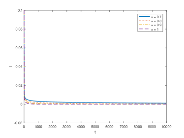
(b) $I(t)$ for $\alpha\in\{0.7,0.8,0.91\}$ and $t\in[0,10000]$.

(c) $C(t)$ for $\alpha\in\{0.7,0.8,0.91\}$ and $t\in[0,10000]$.

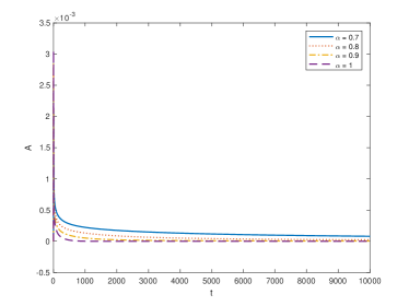
(d) $A(t)$ for $\alpha\in\{0.7,0.8,0.91\}$ and $t\in[0,10000]$.

Figure 1: Stability of the disease free equilibrium $\Sigma_{0}$.

4.2 Stability of the endemic equilibrium $\Sigma_{*}$

For the numerical study of the stability of the endemic equilibrium $\Sigma_{*}$ (7), we consider the parameter values from Table 1 and $\beta=0.01$. The basic reproduction number (6) takes the value $R_{0}=7.95871$. The concrete value of the endemic equilibrium (7) is $\Sigma_{*}=\left(18.3490,8.0673,77.2881,0.6001\right)$. Figure 2 illustrates the stability of the endemic equilibrium for the initial conditions

$$S(0)=100,\quad I(0)=1,\quad C(0)=0,\quad A(0)=0,$$

where a fixed time step size of $h=2^{-6}$ has been used.

(a) $S(t)$ for $\alpha\in\{0.7,0.8,0.91\}$ and $t\in[0,10000]$.

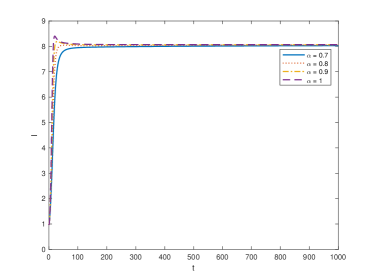
(b) $I(t)$ for $\alpha\in\{0.7,0.8,0.91\}$ and $t\in[0,10000]$.

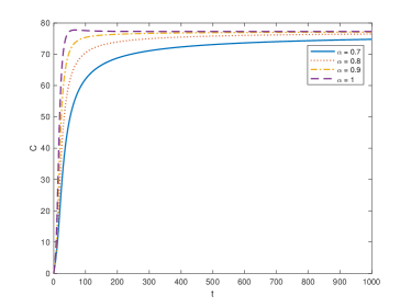
(c) $C(t)$ for $\alpha\in\{0.7,0.8,0.91\}$ and $t\in[0,10000]$.

(d) $A(t)$ for $\alpha\in\{0.7,0.8,0.91\}$ and $t\in[0,10000]$.

Figure 2: Stability of the endemic equilibrium $\Sigma_{*}$.

Our results show that the smaller the order $\alpha$ of the fractional derivative, the slower the convergence to the equilibrium point.

References

- [1]
-
[2]
R. Almeida, S. Pooseh, D. F. M. Torres,
Computational methods in the fractional
calculus of variations, Imperial College Press, London, 2015.
URL https://doi.org/10.1142/p991 -
[3]
A. J. George, A. Chakrabarti,
The Adomian method
applied to some extraordinary differential equations,
Appl. Math. Lett. 8 (3) (1995) 91–97.
URL https://doi.org/10.1016/0893-9659(95)00036-P -
[4]
K. M. Owolabi, A. Atangana,
Spatiotemporal Dynamics of
Fractional Predator–Prey System with Stage Structure for the
Predator, Int. J. Appl. Comput. Math. 3 (suppl. 1) (2017) 903–924.
URL https://doi.org/10.1007/s40819-017-0389-2 -
[5]
E. Ahmed, A. Elgazzar, On
fractional order differential equations model for nonlocal epidemics,
Physica A: Statistical Mechanics and its Applications 379 (2) (2007) 607–614.
URL https://doi.org/10.1016/j.physa.2007.01.010 -
[6]
N. Özalp, E. Demirci, A
fractional order SEIR model with vertical transmission, Math. Comput.
Modelling 54 (1-2) (2011) 1–6.
URL https://doi.org/10.1016/j.mcm.2010.12.051 -
[7]
Y. Guo, The stability of the
positive solution for a fractional SIR model,
Int. J. Biomath. 10 (1) (2017) 1750014, 14 pp.
URL https://doi.org/10.1142/S1793524517500140 -
[8]
Y. Ding, H. Ye, A
fractional-order differential equation model of HIV infection of T-cells, Math. Comput. Modelling 50 (3-4) (2009) 386–392.
URL https://doi.org/10.1016/j.mcm.2009.04.019 -
[9]
E. Ahmed, A. M. A. El-Sayed, H. A. A. El-Saka,
Equilibrium points,
stability and numerical solutions of fractional-order predator-prey
and rabies models,
J. Math. Anal. Appl. 325 (1) (2007) 542–553.
URL https://doi.org/10.1016/j.jmaa.2006.01.087 -
[10]
C. M. A. Pinto, J. A. Tenreiro Machado,
Fractional model for
malaria transmission under control strategies,
Comput. Math. Appl. 66 (5) (2013) 908–916.
URL https://doi.org/10.1016/j.camwa.2012.11.017 -
[11]
C. Li, F. Zhang, A survey on
the stability of fractional differential equations,
The European Physical Journal Special Topics 193 (1) (2011) 27–47.
URL https://doi.org/10.1140/epjst/e2011-01379-1 - [12] M. Rivero, S. V. Rogosin, J. A. Tenreiro Machado, J. J. Trujillo, Stability of fractional order systems, Math. Probl. Eng. (2013) Art. ID 356215, 14 pp.
-
[13]
H. Delavari, D. Baleanu, J. Sadati,
Stability analysis of
Caputo fractional-order nonlinear systems revisited,
Nonlinear Dynam. 67 (4) (2012) 2433–2439.
URL https://doi.org/10.1007/s11071-011-0157-5 -
[14]
N. Aguila-Camacho, M. A. Duarte-Mermoud, J. A. Gallegos,
Lyapunov functions for
fractional order systems,
Commun. Nonlinear Sci. Numer. Simul. 19 (9) (2014) 2951–2957.
URL https://doi.org/10.1016/j.cnsns.2014.01.022 -
[15]
C. Vargas-De-León,
Volterra-type Lyapunov
functions for fractional-order epidemic systems,
Commun. Nonlinear Sci. Numer. Simul. 24 (1-3) (2015) 75–85.
URL https://doi.org/10.1016/j.cnsns.2014.12.013 -
[16]
Y. Wei, H. R. Karimi, S. Liang, Q. Gao, Y. Wang,
General output feedback
stabilization for fractional order systems: an LMI approach,
Abstr. Appl. Anal. (2014) Art. ID 737495, 9 pp.
URL https://doi.org/10.1155/2014/737495 -
[17]
Y. Wei, H. R. Karimi, J. Pan, Q. Gao, Y. Wang,
Observation of a class of
disturbance in time series expansion for fractional order systems,
Abstr. Appl. Anal. (2014) Art. ID 874943, 9 pp.
URL https://doi.org/10.1155/2014/874943 -
[18]
C. J. Silva, D. F. M. Torres,
A TB-HIV/AIDS
coinfection model and optimal control treatment,
Discrete Contin. Dyn. Syst. 35 (9) (2015) 4639–4663.
URL https://doi.org/10.3934/dcds.2015.35.4639 arXiv:1501.03322 -
[19]
C. J. Silva, D. F. M. Torres,
A SICA compartmental
model in epidemiology with application to HIV/AIDS in Cape Verde,
Ecological Complexity 30 (2017) 70–75.
URL https://doi.org/10.1016/j.ecocom.2016.12.001 arXiv:1612.00732 -
[20]
C. J. Silva, D. F. M. Torres,
Global stability
for a HIV/AIDS model,
Commun. Fac. Sci. Univ. Ank. Sér. A1 Math. Stat. 67 (1) (2018) 93–101.
URL https://doi.org/10.1501/Commua1_0000000833 arXiv:1704.05806 -
[21]
S. Rosa, D. F. M. Torres,
Optimal control of a
fractional order epidemic model with application to human respiratory
syncytial virus infection, Chaos Solitons Fractals 117 (2018) 142–149.
URL https://doi.org/10.1016/j.chaos.2018.10.021 arXiv:1810.06900 -
[22]
M. Saeedian, M. Khalighi, N. Azimi-Tafreshi, G. R. Jafari, M. Ausloos,
Memory effects on epidemic
evolution: the susceptible-infected-recovered epidemic model,
Phys. Rev. E 95 (2) (2017) 022409, 9 pp.
URL https://doi.org/10.1103/physreve.95.022409 - [23] D. Matignon, Stability results for fractional differential equations with applications to control processing, in: Computational Engineering in Systems Applications, 1996, pp. 963–968.
- [24] R. Garrappa, Predictor-corrector PECE method for fractional differential equations, MATLAB Central File Exchange (2011) File ID: 32918.
- [25] K. Diethelm, A. D. Freed, The FracPECE subroutine for the numerical solution of differential equations of fractional order, in: S. Heinzel, T. Plesser (Eds.), Forschung und Wissenschaftliches Rechnen 1998, Gessellschaft fur Wissenschaftliche Datenverarbeitung, 1999, pp. 57–71.
- [26] M. Caputo, Linear models of dissipation whose is almost frequency independent. II, Fract. Calc. Appl. Anal. 11 (1) (2008) 4–14, reprinted from Geophys. J. R. Astr. Soc. 13 (1967), no. 5, 529–539.
-
[27]
K. Diethelm, The analysis of
fractional differential equations, Vol. 2004 of Lecture Notes in
Mathematics, Springer-Verlag, Berlin, 2010.
URL https://doi.org/10.1007/978-3-642-14574-2 - [28] I. Podlubny, Fractional differential equations, Vol. 198 of Mathematics in Science and Engineering, Academic Press, Inc., San Diego, CA, 1999.
-
[29]
Y. Li, Y. Chen, I. Podlubny,
Mittag-Leffler
stability of fractional order nonlinear dynamic systems,
Automatica J. IFAC 45 (8) (2009) 1965–1969.
URL https://doi.org/10.1016/j.automatica.2009.04.003 -
[30]
C. J. Silva, D. F. M. Torres,
Modeling and optimal control of
HIV/AIDS prevention through PrEP,
Discrete Contin. Dyn. Syst. 11 (1) (2018) 119–141.
URL https://doi.org/10.3934/dcdss.2018008 arXiv:1703.06446 -
[31]
K. Diethelm, N. J. Ford, A. D. Freed,
Detailed error
analysis for a fractional Adams method, Numer. Algorithms 36 (1) (2004) 31–52.
URL https://doi.org/10.1023/B:NUMA.0000027736.85078.be -
[32]
R. Garrappa, On linear
stability of predictor-corrector algorithms for fractional differential
equations, Int. J. Comput. Math. 87 (10) (2010) 2281–2290.
URL https://doi.org/10.1080/00207160802624331