Radiative contribution to the composite-Higgs potential in a two-representation lattice model

Abstract

Working in a two-representation lattice gauge theory that is close to a composite Higgs model, we calculate the low-energy constant $C_{LR}$ which controls the contribution of the electroweak gauge bosons to the Higgs potential. In QCD, the corresponding low-energy constant governs the mass splitting of the pion multiplet. Taking the continuum and chiral limits, we find that $C_{LR}$, in units of the pseudoscalar decay constant, is roughly of the same size as its QCD counterpart.

I Introduction

Composite Higgs theories of the “Goldstone Higgs” variety Georgi and Kaplan (1984); Dugan et al. (1985) use a weakly broken global symmetry to protect the Higgs from large mass renormalizations. The models are often written down as effective field theories in the form of non-linear sigma models Contino (2011); Bellazzini et al. (2014); Panico and Wulzer (2016). The sigma model describes a set of exactly massless Nambu–Goldstone bosons that live in a coset manifold $G/H$. This set contains the Higgs multiplet of the Standard Model (SM). The Higgs potential then comes mainly from coupling to the electroweak gauge bosons and to the top quark, via one-loop diagrams. This potential should induce the Higgs phenomenon of the SM.

The sigma model is only an effective low-energy description with the correct symmetry properties. The coupling of the Higgs multiplet to the SM fields, which in turn yields the Higgs potential, is given by a number of low-energy constants. These are, in principle, calculable if an ultraviolet completion of the theory is given. We continue here a study of a model that is close to such an ultraviolet theory, one of a set catalogued by Ferretti and Karateev Ferretti and Karateev (2014); Ferretti (2014, 2016); Cacciapaglia et al. (2019) that accommodate both a composite Higgs and a partially composite top quark Kaplan (1991). For that theory, the Higgs potential was discussed in Refs. Golterman and Shamir (2015); Ferretti (2016); Golterman and Shamir (2018).

The model we study is an SU(4) gauge theory containing two multiplets of fermions. The first consists of $N_{f}=2$ Dirac fermions in the sextet representation of SU(4), which is the antisymmetric two-index representation—a real representation. The second contains Dirac fermions in the fundamental representation of SU(4), again with $N_{f}=2$. A Goldstone multiplet arises when the global SU(4) symmetry carried by the sextet fermions is spontaneously broken to SO(4). In Ferretti’s composite Higgs model Ferretti (2014), 5 flavors of Majorana fermions in the sextet representation of SU(4) give rise to a composite Higgs within an SU$(5)/$SO(5) coset. Ferretti’s model also contains fundamental Dirac fermions, but with $N_{f}=3$, to allow construction of a top partner.

When the fermions are weakly coupled to a gauge field outside this model, the Goldstone fields acquire a potential. We present a lattice calculation of the low-energy constant $C_{LR}$ that enters this potential. In Ferretti’s model and in similar theories, the latter is given by Contino (2011); Golterman and Shamir (2014, 2015)

$$V_{\rm eff}(\Sigma)=C_{LR}\sum_{Q}\mathop{\text{tr}}\left(Q\Sigma Q^{*}\Sigma^{*}\right)\ ,$$ (1)

where $\Sigma$ is the non-linear field representing the multiplet of pseudo-Goldstone bosons. The sum over $Q$ runs over the $SU(2)_{L}$ generators $gT^{a}_{L}$ and the hypercharge generator $g^{\prime}Y$, with $g$ and $g^{\prime}$ the electroweak coupling constants of the SM. In accordance with vacuum alignment Peskin (1980), the low-energy constant $C_{LR}$ is positive Witten (1983); Golterman and Shamir (2014), and the minimum of $V_{\rm eff}$ is attained at $\langle\Sigma\rangle={\bf 1}$. The physics of Eq. (1) is analogous to the electromagnetic mass splitting between pions in QCD, a point which we revisit in the discussion. Realization of the Higgs phenomenon requires $V_{\rm eff}$ to have a negative curvature at $\Sigma={\bf 1}$. This is expected to arise from coupling to the top quark Agashe et al. (2005); Ferretti (2014); Golterman and Shamir (2015); Ferretti (2016); Golterman and Shamir (2018), which we do not treat here. For phenomenological use of $C_{LR}$, see for example Ref. Del Debbio et al. (2017).

We obtain $C_{LR}$ in terms of a correlation function of the ultraviolet theory Das et al. (1967),

$$C_{LR}=16\pi^{2}\int\frac{d^{4}q}{(2\pi)^{4}}\,\Pi_{LR}(q_{\mu}).$$ (2)

Here $\Pi_{LR}(q^{2})$ is the transverse part of the current–current correlation function,

$$\frac{1}{2}\delta_{ab}\Pi_{\mu\nu}(q)=-\int{d^{4}x}\,e^{iqx}\,\langle J_{\mu a}^{L}(x)J_{\nu b}^{R}(0)\rangle,$$ (3)

which defines $\Pi_{LR}(q^{2})$ via the decomposition

$$\Pi_{\mu\nu}(q)=(q^{2}\delta_{\mu\nu}-q_{\mu}q_{\nu})\Pi_{LR}(q^{2})+q_{\mu}q_{\nu}\Pi^{\prime}(q^{2}).$$ (4)

The chiral currents, constructed from the sextet fermions, are

$$J^{L}_{\mu a} = \bar{\psi}\gamma_{\mu}(1-\gamma_{5}){T_{a}}\psi=V_{\mu a}-A_{\mu a}\,,$$

$$J^{R}_{\mu a} = \bar{\psi}\gamma_{\mu}(1+\gamma_{5}){T_{a}}\psi=V_{\mu a}+A_{\mu a}\,,$$ (5)

where $T_{a}$ are the isospin generators. In the chiral limit, where the low-energy constant in Eq. (1) is defined, the current correlator (3) is automatically transverse.

In a previous exploratory study, we calculated $C_{LR}$ in the same theory but without the fundamental fermions DeGrand et al. (2016). The present calculation differs from the earlier one in several ways:

1. As noted, we have added fermions in the fundamental representation. This brings the theory closer to Ferretti’s composite Higgs model Ferretti (2014). We do not actually simulate Ferretti’s model for technical reasons, namely, the well-known difficulty of simulating lattice theories with anything other than an even number of Dirac flavors.

2. Exact chirality is important when constructing the currents (5) (see Sec. II). In Ref. DeGrand et al. (2016) we calculated the current correlators with valence overlap fermions. Here we use a more economical prescription, constructing the correlators with valence staggered fermions. The limited chiral symmetry of the latter is enough to guarantee the desired properties of the correlators. (Other calculations of $\Pi_{LR}(q)$ in QCD and beyond Shintani et al. (2008); Boyle et al. (2010); Appelquist et al. (2011) have used overlap or domain-wall fermions. For calculations of the vector current two-point function using staggered fermions, see Refs. Aubin and Blum (2007); Chakraborty et al. (2014, 2017); Borsanyi et al. (2018); Aubin et al. (2018).)

3. Our previous work used only two ensembles, generated with different lattice actions (both based on improved Wilson fermions) but with roughly equal lattice spacings and similar physical properties. While we took a chiral limit for the valence fermions, we did not attempt to take a continuum limit or to extrapolate to the chiral limit of the sea fermions. In this work we measure $C_{LR}$ in ten ensembles with a range of sea masses and lattice spacings. We have studied these ensembles at length Ayyar et al. (2018a, b, c). For each ensemble we have set a scale via the flow variable $t_{0}$ and measured the meson spectrum. Hence we are now able to fit $C_{LR}$ as a function of lattice spacing and sea masses, and to take the continuum and chiral limits in the dynamical theory.

Our paper is organized as follows. In Sec. II we review properties of the current correlation function $\Pi_{LR}$, the importance of chiral symmetry in its calculation, and its definition on the lattice with staggered fermions. In Sec. III we present the calculation of $\Pi_{LR}$ and its integral $C_{LR}$ on each ensemble, along with the extrapolation to massless valence fermions. In Sec. IV we take all the ensembles together in order to fit $C_{LR}$ and extrapolate it to the continuum and chiral limits. We conclude with discussion of our results in Sec. V.

II Chiral symmetry and staggered fermions

II.1 Chiral symmetry

In infinite volume, the value of $C_{LR}$ depends a priori on the dynamical infrared scale $\Lambda$ of the theory, on the fermion mass $m$, and on an ultraviolet cutoff $M$. Chiral symmetry is essential in removing the effects of the ultraviolet cutoff from $C_{LR}$. To see this, we recall DeGrand et al. (2016) the operator product expansion for the two-current correlator, which is, schematically,

$$\Pi_{\textit{XX}}(q^{2};m)\sim 1+\frac{m^{2}}{q^{2}}+\frac{g^{2}\left\langle G_{\mu\nu}G_{\mu\nu}\right\rangle+m\left\langle\bar{\psi}\psi\right\rangle}{q^{4}}+\frac{\Lambda^{6}}{q^{6}}+\cdots\ ,$$ (6)

where $\textit{XX}=VV$ or $AA$. Each term is to be multiplied by a coefficient function that depends logarithmically on $q^{2}$. In the difference $\Pi_{VV}-\Pi_{AA}$, the identity term drops out, as do all purely gluonic condensates, and we have

$$\Pi_{LR}(q^{2};m)\sim\frac{m^{2}}{q^{2}}+\frac{m\Lambda^{3}}{q^{4}}+\frac{\Lambda^{6}}{q^{6}}+\cdots\ ,$$ (7)

where, for each power of $1/q^{2}$, we show only the leading dependence on the fermion mass.

We introduce the ultraviolet cutoff $M$ into Eq. (2) via

$$C_{LR}(m;M)=\int_{0}^{M^{2}}dq^{2}\,q^{2}\,\Pi_{LR}(q^{2};m)\ .$$ (8)

Inserting the expansion (7) we obtain

$$C_{LR}(m;M)\sim m^{2}M^{2}+m\Lambda^{3}\log(M)+\Lambda^{4}+O(1/M^{2}),$$ (9)

where $\Lambda^{4}$ comes from the infrared part of the integral. Hence $C_{LR}(m;M)$ is quadratically divergent for $m\not=0$. Nonetheless, $C_{LR}(0;M)$ is finite in the $M\to\infty$ limit, giving the desired low-energy constant $C_{LR}$. In other words, we must take the (valence) chiral limit before the continuum limit. This result could have been anticipated by noting that $C_{LR}$ is an order parameter for the spontaneous breaking of chiral symmetry.

If the cutoff procedure breaks chiral symmetry, on the other hand, the constant term in Eq. (6) does not cancel between $VV$ and $AA$, and $C_{LR}(m\to 0)$ remains (quartically) divergent. Thus it is important to use chiral valence fermions in defining the currents on the lattice. In our numerical calculation we use a discretized version of Eq. (2). We impose an upper limit $M$ in the summation over momenta, along the lines of Eq. (8), with $M<\pi/a$. For non-zero valence mass $m_{v}$, one expects the dependence of $C_{LR}(m_{v};M)$ to contain a quadratically divergent term $\sim m_{v}^{2}/a^{2}$; this dependence should vanish when $m_{v}\to 0$.

II.2 Lattice

We have seen that we require an axial current that is exactly conserved in the chiral limit. In our previous work DeGrand et al. (2016), we chose to use overlap fermions for this purpose. Here, for reasons of economy, we work with staggered fermions. The conserved U(1) vector current is (see for example Ref. DeGrand and DeTar (2006))

$$V_{\mu}(x)=\frac{\eta_{\mu}(x)}{2}\left(\bar{\chi}(x)U_{\mu}(x)\chi(x+\hat{\mu})+\bar{\chi}(x+\hat{\mu})U^{\dagger}_{\mu}(x)\chi(x)\right),$$ (10)

while the partially conserved $\textrm{U}(1)_{\epsilon}$ axial current is

$$A_{\mu}(x)=\frac{\eta_{\mu}(x)\epsilon(x)}{2}\left(\bar{\chi}(x)U_{\mu}(x)\chi(x+\hat{\mu})-\bar{\chi}(x+\hat{\mu})U^{\dagger}_{\mu}(x)\chi(x)\right)\ .$$ (11)

The sign factors are, as usual,

$$\eta_{1}(x)=1\ ,\quad\eta_{2}(x)=(-1)^{x_{1}}\ ,\quad\eta_{3}(x)=(-1)^{x_{1}+x_{2}}\ ,\quad\eta_{4}(x)=(-1)^{x_{1}+x_{2}+x_{3}}\ ,$$ (12)

and $\epsilon(x)=(-1)^{x_{1}+x_{2}+x_{3}+x_{4}}$. These currents correspond to the nearest-neighbor staggered action. The vector current satisfies the continuity equation

$$\sum_{\mu}\partial^{-}_{\mu}V_{\mu}(x)=\sum_{\mu}\Big{(}V_{\mu}(x)-V_{\mu}(x-\hat{\mu})\Big{)}=0\ ,$$ (13)

and the axial current satisfies a similar continuity equation in the massless limit.

We calculate the current–current correlation function $\Pi_{LR}(q)$ with the staggered currents (10), (11) exactly as was done with the overlap currents in Ref. DeGrand et al. (2016). Writing the chiral currents,

$$J^{L}_{\mu a} = V_{\mu a}-A_{\mu a}\,,$$

$$J^{R}_{\mu a} = V_{\mu a}+A_{\mu a}\,,$$ (14)

we define the lattice correlator,

$$\frac{1}{2}\delta_{ab}\Pi_{\mu\nu}^{\textrm{lat}}(q)=-\frac{1}{4}a^{4}\sum_{x}\,e^{iqx}\,\left\langle J_{\mu a}^{L}(x)J_{\nu b}^{R}(0)\right\rangle\ .$$ (15)

The factor of $\frac{1}{4}$ corrects for the summation over the four tastes inherent in the staggered field. The $\frac{1}{2}$ is the normalization of isospin generators, $\mathop{\text{tr}}T_{a}T_{b}=\frac{1}{2}\delta_{ab}$. As usual, $q_{\mu}=(2\pi/L_{\mu})n_{\mu}$ for periodic boundary conditions with period $L_{\mu}$, where $-N_{\mu}/2<n_{\mu}\leq N_{\mu}/2$. The desired $\Pi_{LR}(q)$ is the transverse piece of the correlation function. We use a lattice definition,

$$\Pi_{LR}(q)=\frac{\sum_{\mu\nu}P^{T}_{\mu\nu}(q)\Pi^{\textrm{lat}}_{\mu\nu}(q)}{3(\hat{q}^{2})^{2}},$$ (16)

that uses the lattice projector,

$$P^{T}_{\mu\nu}(q)=\hat{q}^{2}\delta_{\mu\nu}-\hat{q}_{\mu}\hat{q}_{\nu}\ ,$$ (17)

where $\hat{q}_{\mu}=(2/a)\sin(q_{\mu}a/2)$ and $\hat{q}^{2}\equiv\sum_{\mu}\hat{q}_{\mu}^{2}$. Any lattice projector of course introduces lattice artifacts. Their effects will vanish when we take the continuum limit.

III Lattice calculations

Our results are based on the measurement of $\Pi_{LR}(q)$ on ten ensembles, to be described below. In this section we give the methods applied to each ensemble separately, using one ensemble for illustration. First we present our smearing procedure and describe its effect on the taste spectrum, as a function of the valence mass $m_{v}$. Then we present $\Pi_{LR}(q)$ and compare it to a physical model, the minimal hadron approximation. Finally, using values of $f_{\pi}$ obtained from valence spectroscopy, we calculate $C_{LR}(m_{v})$ from $\Pi_{LR}$ and take the chiral limit, $m_{v}\to 0$, for the staggered valence fermions on each ensemble. We combine the ensemble results in Sec. IV, giving a fit for $C_{LR}$ where the independent variables are the lattice spacing and the masses of the two sea fermions, measured in each ensemble; this fit produces continuum and chiral limits for $C_{LR}$.

III.1 Overview of the ensembles

We base this study on 10 ensembles created for previous work. They were generated with a lattice action containing an SU(4) gauge field coupled to dynamical fermions in both the fundamental 4 and the two-index antisymmetric 6 representation of SU(4), with two Dirac flavors of each. For the fermions we use a Wilson-clover action, with normalized hypercubic (nHYP) smeared gauge links Hasenfratz and Knechtli (2001); Hasenfratz et al. (2007). The clover coefficient is set equal to unity for both fermion species Bernard and DeGrand (2000); Shamir et al. (2011). The pure gauge part of the action is the usual plaquette term plus an nHYP dislocation-suppressing (NDS) term, a smeared action designed to reduce gauge-field roughness that would create large fermion forces in the molecular dynamics evolution DeGrand et al. (2014).

The ensembles have lattice volumes of $N_{s}^{3}\times N_{t}=16^{3}\times 32$ and $24^{3}\times 48$. They were generated and first used to calculate the meson spectrum of this model Ayyar et al. (2018a). Twelve ensembles with volume $16^{3}\times 32$ were then used to calculate the baryon spectrum, including mixed-representation “chimera” baryons Ayyar et al. (2018b); a subset of these was used in calculating matrix elements of baryonic currents, in connection with partial compositeness Ayyar et al. (2018c). In the present calculation of $C_{LR}$ we use nine of the $16^{3}\times 32$ ensembles and one ensemble of volume $24^{3}\times 48$.

Details relating to the ensembles appear in Appendix A. Table 2 gives the values of the bare parameters used to generate the ensembles: the gauge coupling $\beta$ and the two hopping parameters, $\kappa_{4}$ and $\kappa_{6}$, for the two fermion types. We connect them to physics by the calculated values of the flow parameter $t_{0}/a^{2}$ and the fermion masses $m_{4}a$ and $m_{6}a$, obtained from the axial Ward identities (AWI). We use $t_{0}$ for setting the scale Ayyar et al. (2018a) (for example, $t_{0}\simeq(1.4\ \textrm{GeV})^{-2}$ in QCD), whence we define the dimensionless lattice spacing $\hat{a}=a/\sqrt{t_{0}}$ for each ensemble and the dimensionless AWI masses $\hat{m}_{4}=m_{4}\sqrt{t_{0}}$ and $\hat{m}_{6}=m_{6}\sqrt{t_{0}}$, as well as $\hat{C}_{LR}=C_{LR}\,t_{0}^{2}$. We will use these quantities in taking continuum and chiral limits. The measured values for these quantities appear in Table 3. We refer the reader to Refs. Ayyar et al. (2018a, b) for more information about the ensembles.

III.2 Staggered valence fermions: smearing and the taste spectrum

As discussed above, in order to maintain an exact chiral symmetry, we calculate valence propagators with a staggered fermion action. We use a nearest-neighbor action, improved by smearing the SU(4) gauge field before promoting it to the sextet representation. As in the Wilson action of the sea fermions, the smearing is an nHYP scheme; the smearing parameters are the same for the valence and the sea fermions. In an effort to reduce lattice artifacts, we smear more than once to derive the valence action. We calculate the valence propagators for seven values of the valence mass for all the ensembles, with $0.01\leq m_{v}a\leq 0.05$.

Figure 1: Squared mass $(m_{\pi}a)^{2}$ of the valence Goldstone pion and the seven additional pion multiplets, constructed from the staggered valence fermions, in ensemble 2. The abscissa is $m_{v}a$, the valence fermion mass. The four plots correspond to $s=1$, 2, 3, and 4 levels of smearing, carried out on the gauge field configurations before calculating the fermion propagators. The lines connect points of each multiplet. The Goldstone pion is always the bottom curve.

Figure 1 shows the splitting of the eight pion multiplets (that differ in their internal taste structure Golterman (1986); Lee and Sharpe (1999)) in ensemble 2, calculated with one to four levels of smearing. Going from one to two levels of smearing dramatically reduces the taste splittings, while additional smearing produces only marginal improvement. The slope of the Goldstone pion’s mass squared, which is a low energy constant, also changes only slightly after two smearings. For production, we stop at two smearing levels, for two reasons.

1. We eventually combine the ensembles to arrive at a continuum extrapolation. There is no reason to eliminate lattice artifacts before then; we only require them to be small enough that they do not hamper the extrapolation.

2. Repeated smearing increases the range of the action. This may introduce a sensitivity to the finite volume.

III.3 Minimal hadron approximation and $f_{\pi}$

The minimal hadron approximation (MHA) provides a physically appealing interpretation of $\Pi_{LR}(q)$ at low momentum. The MHA supposes that $\Pi_{LR}(q)$ may be modeled by retaining poles from the pion and the lightest states in the axial and vector channels (the analogues of the $a_{1}$ and $\rho$ mesons in QCD, respectively):

$$\Pi_{LR}(q)\approx\frac{f_{\pi}^{2}}{q^{2}}+\frac{f_{a_{1}}^{2}}{q^{2}+m_{a_{1}}^{2}}-\frac{f_{\rho}^{2}}{q^{2}+m_{\rho}^{2}}\,.$$ (18)

The first term comes from applying the transverse projection to the $f_{\pi}$-dependent term in the current correlator and does not depend the pion mass (see Ref. DeGrand et al. (2016)). We conducted fits to this function on each ensemble. For illustration, Fig. 2 shows $\hat{q}^{2}\Pi_{LR}(\hat{q})$ calculated and fit for each valence mass $m_{v}$ for ensemble 2. We fit to data in the range $\hat{q}^{2}<0.5$, since the MHA is only expected to hold at low momentum. The figure shows that the fit works well at least up to $\hat{q}^{2}=1$.

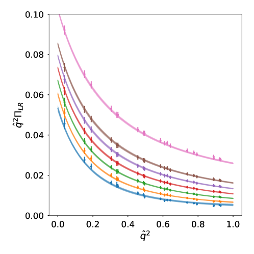
Figure 2: The transverse part $\Pi_{LR}$ of the current–current correlation function, plotted against $\hat{q}^{2}=\sum_{\mu}\hat{q}_{\mu}^{2}$, in ensemble 2. We plot the data and the fit to the MHA for the seven values of the valence mass $m_{v}=0.05$, 0.035, 0.03, 0.025, 0.02, 0.015, 0.01, top to bottom.

We can compare the value of $f_{\pi}$ emerging from the fit to Eq. (18) to the spectroscopic value of $f_{\pi}$, which we calculate from the correlation function of the pseudoscalar density,

$$-a^{3}\sum_{\bf x}\left\langle P^{a}({\bf x},t)P^{b}({\bf 0},0)\right\rangle=4\,\frac{f_{\pi}^{2}m_{\pi}^{3}}{8m_{q}^{2}}\,\delta^{ab}e^{-m_{\pi}t},$$ (19)

where $a,b$ are isospin indices and (again) the factor of 4 is for the four staggered tastes. In our previous work DeGrand et al. (2016), we found that these two values for $f_{\pi}$ match closely, for both ensembles studied there. We compare the two determinations of $f_{\pi}$ in Fig. 3, which is typical of all our ensembles. The discrepancies are a combination of the limitations of the three-pole ansatz and scaling violations. We also show $f_{P6}$, the decay constant of the dynamical sextet Wilson pions, calculated in Ref. Ayyar et al. (2018a). Its rough agreement with the valence values suggests that the added discretization error due to the use of a mixed action, coming from the difference in the finite parts of renormalization constants, is not large.

In Ref. DeGrand et al. (2016) we calculated $C_{LR}$ by integrating the MHA fit as well as by direct summation of $\Pi_{LR}$ in momentum space. The MHA fits worked surprisingly well even in the UV regime, allowing us to use them for the complete momentum integral. In the current work, we find that the fits do not work well at momenta outside the plot in Fig. 2, perhaps because of large discretization effects in the staggered formalism. Hence, in Sec. III.4 below, we discard the MHA fits in favor of direct summation. Moreover, we use the spectroscopic value of $f_{\pi}$ rather than that which emerges from the MHA fit.

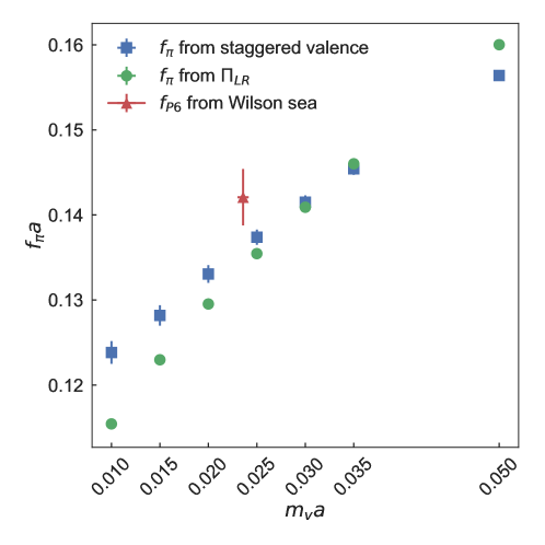
Figure 3: Comparison of $f_{\pi}$, the decay constant of the sextet valence pions, calculated from the MHA fit to $\Pi_{LR}(q)$, to that calculated directly from Eq. (19) in ensemble 2. The abscissa is the mass of the valence fermions. The error bars of the green circles are smaller than the symbols. Also shown is $f_{P6}$, the decay constant of the sextet pions in the Wilson sea. For this, the abscissa is the sextet AWI mass measured in the ensemble.

III.4 $C_{LR}(m_{v})$ and the valence chiral limit

To calculate $C_{LR}(m_{v})$ on each ensemble, we follow the method of Ref. DeGrand et al. (2016). We compute the four-dimensional integral in Eq. (2) as direct summation of $\Pi_{LR}(q_{\mu})$ in discrete momentum space. The discrete version of Eq. (2) is

$$C_{LR}=\frac{16\pi^{2}}{V}\sum_{q_{\mu}}\Pi_{LR}(q_{\mu}),$$ (20)

where $V=L_{s}^{3}L_{t}$. A sum over the entire Brillouin zone of the lattice would run over momenta $|q_{\mu}a|<\pi$, in steps of $\Delta q_{\mu}a=2\pi/N_{\mu}$. In the present analysis with staggered fermions, such a sum would include contributions from the Brillouin zone face that represent currents with various (adjoint) taste structures in the continuum limit. We limit the summation in Eq. (20) to the “reduced Brillouin zone,”

$$|q_{\mu}a|\leq q_{\textrm{max}}a=\pi/2,$$ (21)

or to a subset thereof (see below). This retains only the taste-singlet vector current and the partially conserved axial current, which contains $\gamma_{5}\xi_{5}$ in Dirac-taste space. With any prescription for the momentum sum, the lattice defines the divergent part of $C_{LR}(m_{v})$ when $m_{v}$ is nonzero, proportional to $m_{v}^{2}/a^{2}$.

Equation (20) requires special care at the origin of momentum space. In the first place, the transverse projection (16) is undefined at $q=0$; in the second place, $\Pi_{LR}$ in the continuum contains a kinematical pole at $q=0$ (as is seen, for instance, in the MHA). Near zero, then, we approximate the continuum function as

$$\Pi_{LR}(q_{\mu})\simeq\frac{f_{\pi}^{2}}{q^{2}}+p,$$ (22)

where we take the value of $f_{\pi}$ from the spectroscopic data and estimate the pedestal $p$ from $m$ neighboring momenta (see Ref. DeGrand et al. (2016)),

$$p=\frac{1}{m}\sum_{a=1}^{m}\left(\Pi_{LR}(q^{a})-\frac{f_{\pi}^{2}}{(q^{a})^{2}}\right).$$ (23)

That is, $p$ is the average of the discrete $\Pi_{LR}$ in the neighboring cells, minus the pole term on those cells. The contribution of $q=0$ to the discrete summation (20) is then

$$A\frac{L_{s}^{2}}{V}\,f_{\pi}^{2}+\frac{16\pi^{2}}{V}p,$$ (24)

where $A\circeq 22.5095963$ is a geometric factor calculated for the aspect ratio of our lattices, $L_{t}/L_{s}=2$.

Figure 4: The low-energy constant $C_{LR}$ plotted against the valence mass $m_{v}$ (both in lattice units) in ensemble 2. The three sets of data and the corresponding curves come from three different high-momentum cutoffs in the summation (20). The points plotted at $m_{v}=0$ (slightly shifted) are the cubic extrapolations of the data to zero. The correlated errors are calculated from single-elimination jackknife.

Figure 4 shows the results for $C_{LR}(m_{v})$ for ensemble 2, together with a cubic fit extrapolating to $m_{v}=0$. The top set of points corresponds to the summation (20) over the entire reduced Brillouin zone, Eq. (21). The extrapolation reaches $m_{v}=0$ at the point plotted slightly to the left of zero. To examine the effect of the UV cutoff, we drop the highest momenta in the reduced Brillouin zone. Because ensemble 2 has volume $16^{3}\times 32$, this amounts to decreasing

$$q_{\textrm{max}}a\rightarrow\frac{\pi}{2}-\frac{2\pi}{N_{s}}=\frac{3\pi}{8}.$$ (25)

The resulting values for $C_{LR}(m_{v})$ give the middle data set and curve in Fig. 4, extrapolated to the point plotted exactly at $m_{v}=0$. As a third variation, we decrease the cutoff further, $q_{\textrm{max}}a\rightarrow{\pi}/{4}$, which gives the bottom data set and curve, extrapolated to the point plotted slightly to the right of zero. The result of varying the UV cutoff is as expected: There is a marked change for nonzero valence mass, while $C_{LR}(0)$ is unchanged given the error bar.

The corresponding results for all the ensembles are quite similar. The $\chi^{2}/\textrm{dof}$ of each fit is in the neighborhood of 0.3 for all ensembles. We list the extrapolated $C_{LR}(0)$ in Table 1. The use of a cubic for this fit, though arbitrary, gives an extrapolation that is stable under changes in the fitting polynomial. Chiral perturbation theory, which gives formulas for many quantities, is not helpful here. It can only treat $\Pi_{LR}(q)$ at low $q^{2}$, and hence it does not give a useful formula for $C_{LR}(m_{v})$.

The extrapolation to $m_{v}=0$ also offers a means to test for sensitivity to finite-volume effects in $C_{LR}$. Regarding mesonic quantities based on the sea fermions, the possibility of finite-volume contamination was addressed at length in Ref. Ayyar et al. (2018a) and dismissed. The new ingredient in this work is the light valence fermions. Finite-volume effects would of course be strongest for the smallest values of $m_{v}$. A simple test is thus to drop the smallest values and examine anew the extrapolation of $C_{LR}$ to $m_{v}=0$. We find that dropping the two smallest masses, $m_{v}=0.01$ and 0.015, shifts each extrapolation by less than its error bar. Given the small $\chi^{2}$ of each fit, this is not surprising. Moreover, the fits show no sign of requiring a term proportional to $1/(m_{v}\sqrt{V})$, an expected consequence of zero modes in a partially quenched theory. See Ref. DeGrand et al. (2016) for more discussion.

While chiral perturbation theory is not directly applicable to $C_{LR}$ itself, one could argue that it can be used to understand the finite-volume correction to $C_{LR}$, which is a large-distance quantity Aubin et al. (2016). In our mixed-action setup, finite-volume corrections are controlled by the mass $M_{vs}$ of the mixed (valence-sea) pion. The latter satisfies the bound Bär et al. (2011)

$$M_{vs}^{2}\geq(M_{ss}^{2}+M_{vv}^{2})/2\ .$$ (26)

where $M_{ss}$ and $M_{vv}$ are respectively the masses of the pure sea and valence pions. For ensemble 2 we can read $M_{vv}$ off Fig. 1 and $M_{ss}$ from Table 3 (the sextet pion mass $M_{P6}$). We find that $M_{vs}L_{s}\geq 3.9$ when the smallest valence mass is 0.01, and $M_{vs}L_{s}\geq 4.4$ when it is 0.02. In all other ensembles $M_{vs}L_{s}$ satisfies more stringent bounds. The increase of $M_{vs}L_{s}$ from (at least) 3.9 to (at least) 4.4 thus lends further support to our conclusion that finite-volume effects are negligible, within the precision of our calculation.

Ensemble	$C_{LR}a^{4}$
2	0.0103(11)
3	0.0081(10)
4	0.0120(8)
5	0.0057(6)
6	0.0217(16)
8	0.0037(6)
9	0.0096(7)
11	0.0028(6)
12	0.0027(6)
40	0.0036(3)

Table 1: The low-energy constant $C_{LR}$, calculated via summation over the entire reduced Brillouin zone, extrapolated to zero valence mass.

IV $C_{LR}$ in the chiral and continuum limit

The ultimate goal of this study is the value of the low-energy constant $C_{LR}$ in the continuum limit. As discussed above, $C_{LR}$ is finite and therefore physical only in the chiral limit of the sextet fermion. In the present partially quenched lattice calculation, unitarity requires a simultaneous chiral limit for the sea and valence sextet fermions. Therefore, the sole free parameter in the continuum limit is the mass of the fundamental fermions. In Sec. III.4 we took the chiral limit for the valence sextet fermions. We now turn our attention to the continuum limit and chiral limit for the sextet sea fermions.

To conduct this joint limit, we consider the dimensionless product $\hat{C}_{LR}=C_{LR}t_{0}^{2}$. We model our data with a simple linear function,

$$\hat{C}_{LR}=p_{0}+p_{a}\hat{a}+p_{6}\hat{m}_{6},$$ (27)

which neglects dependence on the fundamental fermion mass $\hat{m}_{4}$. Later we test the stability of the fit parameters against alternative models, e.g., including dependence on the fundamental fermion mass. First, we construct jackknife correlation matrices among the lattice quantities $C_{LR}$, $m_{4}$, and $m_{6}$ on each ensemble. We do not include correlations with the flow scale $t_{0}/a^{2}$ (i.e., with $\hat{a}\equiv a/\sqrt{t_{0}}$ Ayyar et al. (2018a)), which has negligible error compared to the other quantities we extract. We then conduct a correlated fit to Eq. (27), obtaining $p_{0}=0.028(4)$, $p_{a}=-0.021(4)$, and $p_{6}=0.16(3)$, for $\chi^{2}=9.2/7$ dof.

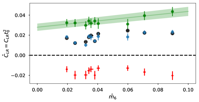
Figure 5: Fit of $\hat{C}_{LR}$ to Eq. (27). The data appear in blue. The best fit is in hollow black points. The lattice artifact term $p_{a}\hat{a}$ from Eq. (27) identified by the fit appears in red. The green points show the data minus the lattice artifact. The smooth green band shows the continuum prediction, i.e., Eq. (27) minus the $p_{a}\hat{a}$ term.

Figure 5 displays the result of the fit. The hollow black points show the fit at the values of $\hat{a}$ and $\hat{m}_{6}$ of the individual ensembles; they follow the solid blue data points closely. The lattice artifacts [$(p_{a}\hat{a})$ from Eq. (27)] identified by the fit appear in red. The green points show the data minus the lattice artifact. According to the model, subtracting the artifacts from the full fit yields a linear function of $\hat{m}_{6}$, which is displayed as a green band. This band represents the continuum limit.

It is significant that the fit, Eq. (27), works so well without including any dependence on $\hat{m}_{4}$, the mass of the fundamental fermions. We have found before that the fundamental fermions have only a weak influence on quantities constructed from the sextet fermions Ayyar et al. (2018a, b). We can test the stability of our fit against the inclusion of an $\hat{m}_{4}$ term, as well as higher-order terms in $\hat{m}_{6}$ and $\hat{a}$:

$$\hat{C}_{LR}=p_{0}+p_{a}\hat{a}+p_{6}\hat{m}_{6}+p_{4}\hat{m}_{4}+p_{66}\hat{m}_{6}^{2}+p_{a6}\hat{a}\hat{m}_{6}+p_{aa}\hat{a}^{2}\ .$$ (28)

Figure 6 shows the stability of the best-fit result $p_{0}$ under the inclusion of these additional terms. No significant discrepancy is seen; the largest deviation comes from the fit “$\textrm{Base}-p_{a}+p_{aa}$,” which models the lattice-spacing dependence as quadratic instead of linear. As can be seen from Fig. 5, although the lattice-artifact contributions are significant, they vary little over the set of ensembles considered, which makes it difficult to determine whether linear or quadratic dependence on $\hat{a}$ is a more appropriate description of our results.

The fit including the quadratic $p_{aa}$ yields a best-fit value of $p_{0}=0.020(2)$, as compared to the result $p_{0}=0.028(4)$ from the base fit. Since we cannot reject either hypothesis, we conservatively adopt half of the difference in central values between these two fits as a systematic error, giving our final result

$$\hat{C}_{LR}=0.024(4)_{\rm stat}(4)_{\rm sys}\ .$$ (29)

This is the chiral limit $m_{v}=m_{6}=0$ in both valence and sea-sextet masses, as well as the continuum limit, of $\hat{C}_{LR}$.

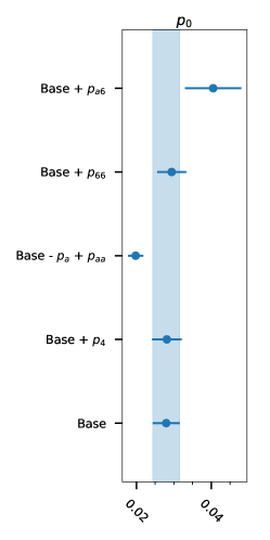
Figure 6: Stability of the fit parameter $p_{0}$ under model variations. The shaded band corresponds to the fit to the base model of Eq. (27), shown in the bottom row. The alternative models include additional terms shown in Eq. (28).

V Discussion

In this paper we computed the low-energy constant $C_{LR}$ for the sextet representation. We used staggered valence fermions to define the currents, instead of overlap fermions as in our previous work. We indeed found this to be an economical way to impose exact chiral symmetry. On the other hand, we find a strong dependence of $C_{LR}(m_{v},M)$ on the cutoff momentum $M$, when the valence mass $m_{v}$ is nonzero. When using overlap fermions, we could not resolve any dependence at all on $M$. In any case, the divergent cutoff dependence disappears in the valence chiral limit, as expected for the quadratic divergence $m_{v}^{2}M^{2}\sim m_{v}^{2}/a^{2}$.

Taking the continuum limit as well as the chiral limit for both sea and valence sextet fermions we find $\hat{C}_{LR}=C_{LR}t_{0}^{2}=0.024(4)(4)$. Within error, this result turns out to be independent of the mass of the fundamental fermions, for the mass range covered by our ensembles. To simplify the lattice calculation we have considered a fermion content that is slightly different from Ferretti’s model, so that our result is not directly applicable. We expect, however, that our result for $C_{LR}$ will be numerically similar to that in Ferretti’s actual model.

In Ferretti’s model, the ratio $C_{LR}/f_{P6}^{4}$, where $f_{P6}$ is the sextet pseudoscalar decay constant, controls the contribution of the electroweak gauge bosons to the Higgs potential. From Ayyar et al. (2018a), the value of $f_{P6}$ in the sextet chiral limit is $\sqrt{t_{0}}f_{P6}=0.17(1)$. Our determinations of $C_{LR}$ and $f_{P6}$ are found to be weakly correlated, so we can take the ratio and combine the errors in quadrature, finding the result

$$\frac{C_{LR}}{f_{P6}^{4}}=29(8)(5)\ .$$ (30)

In the notation of Del Debbio et al. (2017), this result translates to $\hat{c}_{LR}=\frac{1}{2}(3g^{2}+g^{\prime}{}^{2})(C_{LR}/f_{P6}^{4})=19(5)(3)$. Certain combinations of $\hat{c}_{LR}$ with other low-energy constants in the theory must be of order $10^{-2}$ to reproduce the observed properties of the Higgs boson, so this result implies some amount of fine-tuning in the theory.

It is interesting to compare our result with QCD. Das et al. Das et al. (1967) showed long ago that the electromagnetic mass splitting among pions is given by

$$m_{\pi^{\pm}}^{2}-m_{\pi^{0}}^{2}=\frac{3\alpha}{4\pi}\frac{C_{LR}}{f_{\pi}^{2}}\ .$$ (31)

Solving for $C_{LR}$ in terms of the experimental values gives, for QCD, $C_{LR}\approx 0.012~{}\text{GeV}^{4}$, and $C_{LR}/f_{\pi}^{4}\approx 42$, where our convention for the decay constant is $f_{\pi}\simeq 130~{}\text{MeV}$. Our result in the present model is thus comparable with the QCD value. Expectations from large-$N_{c}$ Ayyar et al. (2018a) are that $C_{LR}$ should scale as the dimension of the representation, i.e., similar to $f_{P6}^{2}$. The dimension of the antisymmetric representation is $N_{c}(N_{c}-1)/2$, and so our smaller value for $C_{LR}/f_{P6}^{4}$ is in rough agreement with such scaling, too.

We have recently computed the top-quark mass induced via partial compositeness in this model, finding it to be too small by several orders of magnitude. This makes it extremely unlikely that Ferretti’s model could generate a realistic top mass Ayyar et al. (2018c). However, the model might be rescued by introducing additional fermion species which are inert under all Standard Model interactions. These will slow down the running, ultimately producing a nearly conformal but confining theory, which, in principle, might allow for large enhancement of the induced top mass. Other models from the Ferretti-Karateev list Ferretti and Karateev (2014) might give a more realistic top mass as well Bennett et al. (2018); Lee et al. (2018).

Appendix A The ensembles

Table 2 lists the ensembles used in this study. The nine ensembles labelled 2–12 are lattices with volume $16^{3}\times 32$, numbered as in Ref. Ayyar et al. (2018b) for easy reference; ensemble 40 has volume $24^{3}\times 48$ (see Ref. Ayyar et al. (2018a)). We have excluded ensembles (1, 7, 10) because large fluctuations in the observable $C_{LR}(m_{v})$ indicate that the simulations are much too short. Of our $24^{3}\times 48$ ensembles, only ensemble 40 avoids this problem.

Table 3 presents some physical properties of the ensembles. These are the flow parameter $t_{0}$; the fermion masses from the axial Ward identities, rendered dimensionless as $\hat{m}_{4}=m_{4}\sqrt{t_{0}}$, and $\hat{m}_{6}=m_{6}\sqrt{t_{0}}$; and the pseudoscalar meson masses, $\hat{M}_{P4}=M_{P4}\sqrt{t_{0}}$ and $\hat{M}_{P6}=M_{P6}\sqrt{t_{0}}$.

Ensemble	$\beta$	$\kappa_{4}$	$\kappa_{6}$	Configurations
2	7.25	0.13147	0.13395	71
3	7.30	0.13117	0.13363	61
4	7.30	0.13162	0.1334	71
5	7.55	0.13	0.1325	85
6	7.65	0.129	0.1308	50
8	7.65	0.13	0.132	85
9	7.75	0.128	0.131	85
11	7.75	0.1295	0.1315	34
12	7.85	0.129	0.1308	45
40	7.51	0.1307	0.1328	133

Table 2: The ensembles used in this study. The lattice volumes are $16^{3}\times 32$ (ensembles 2–12) and $24^{3}\times 48$ (ensemble 40).

Ensemble	$t_{0}/a^{2}$	$\hat{m}_{4}$	$\hat{m}_{6}$	$\hat{M}_{P4}$	$\hat{M}_{P6}$
2	1.135(9)	0.028(1)	0.025(1)	0.305(9)	0.303(8)
3	1.13(1)	0.0345(8)	0.032(1)	0.340(5)	0.340(9)
4	1.111(9)	0.0228(6)	0.0381(8)	0.279(7)	0.368(11)
5	1.85(2)	0.050(1)	0.034(1)	0.429(10)	0.375(9)
6	1.068(5)	0.082(1)	0.0896(8)	0.514(8)	0.576(9)
8	2.29(2)	0.038(1)	0.036(2)	0.400(9)	0.408(10)
9	1.56(1)	0.108(1)	0.071(1)	0.636(7)	0.538(8)
11	2.62(2)	0.047(1)	0.040(1)	0.443(14)	0.428(15)
12	2.67(2)	0.060(1)	0.060(1)	0.505(13)	0.529(17)
40	2.26(2)	0.0196(4)	0.0194(9)	0.278(4)	0.291(10)

Table 3: Physical properties of the ensembles: Flow variable $t_{0}$, AWI masses $\hat{m}_{r}=m_{r}\sqrt{t_{0}}$, and pseudoscalar meson masses $\hat{M}_{Pr}=M_{Pr}\sqrt{t_{0}}$ for dynamical fermions in representations $r=4,6$.

References

- Georgi and Kaplan (1984) H. Georgi and D. B. Kaplan, Phys. Lett. 145B, 216 (1984).
- Dugan et al. (1985) M. J. Dugan, H. Georgi, and D. B. Kaplan, Nucl. Phys. B254, 299 (1985).
- Contino (2011) R. Contino, in Physics of the large and the small, TASI 09, proceedings of the Theoretical Advanced Study Institute in Elementary Particle Physics, Boulder, Colorado, USA, 1-26 June 2009 (2011) pp. 235–306, arXiv:1005.4269 [hep-ph] .
- Bellazzini et al. (2014) B. Bellazzini, C. Csáki, and J. Serra, Eur. Phys. J. C74, 2766 (2014), arXiv:1401.2457 [hep-ph] .
- Panico and Wulzer (2016) G. Panico and A. Wulzer, Lect. Notes Phys. 913 (2016), arXiv:1506.01961 [hep-ph] .
- Ferretti and Karateev (2014) G. Ferretti and D. Karateev, JHEP 03, 077 (2014), arXiv:1312.5330 [hep-ph] .
- Ferretti (2014) G. Ferretti, JHEP 06, 142 (2014), arXiv:1404.7137 [hep-ph] .
- Ferretti (2016) G. Ferretti, JHEP 06, 107 (2016), arXiv:1604.06467 [hep-ph] .
- Cacciapaglia et al. (2019) G. Cacciapaglia, G. Ferretti, T. Flacke, and H. Serôdio, Front. Phys. 7, 22 (2019), arXiv:1902.06890 [hep-ph] .
- Kaplan (1991) D. B. Kaplan, Nucl. Phys. B365, 259 (1991).
- Golterman and Shamir (2015) M. Golterman and Y. Shamir, Phys. Rev. D91, 094506 (2015), arXiv:1502.00390 [hep-ph] .
- Golterman and Shamir (2018) M. Golterman and Y. Shamir, Phys. Rev. D97, 095005 (2018), arXiv:1707.06033 [hep-ph] .
- Golterman and Shamir (2014) M. Golterman and Y. Shamir, Phys. Rev. D89, 054501 (2014), arXiv:1401.0356 [hep-lat] .
- Peskin (1980) M. E. Peskin, Nucl. Phys. B175, 197 (1980).
- Witten (1983) E. Witten, Phys. Rev. Lett. 51, 2351 (1983).
- Agashe et al. (2005) K. Agashe, R. Contino, and A. Pomarol, Nucl. Phys. B719, 165 (2005), arXiv:hep-ph/0412089 [hep-ph] .
- Del Debbio et al. (2017) L. Del Debbio, C. Englert, and R. Zwicky, JHEP 08, 142 (2017), arXiv:1703.06064 [hep-ph] .
- Das et al. (1967) T. Das, G. S. Guralnik, V. S. Mathur, F. E. Low, and J. E. Young, Phys. Rev. Lett. 18, 759 (1967).
- DeGrand et al. (2016) T. A. DeGrand, M. Golterman, W. I. Jay, E. T. Neil, Y. Shamir, and B. Svetitsky, Phys. Rev. D94, 054501 (2016), arXiv:1606.02695 [hep-lat] .
- Shintani et al. (2008) E. Shintani, S. Aoki, H. Fukaya, S. Hashimoto, T. Kaneko, H. Matsufuru, T. Onogi, and N. Yamada (JLQCD), Phys. Rev. Lett. 101, 242001 (2008), arXiv:0806.4222 [hep-lat] .
- Boyle et al. (2010) P. A. Boyle, L. Del Debbio, J. Wennekers, and J. M. Zanotti (RBC, UKQCD), Phys. Rev. D81, 014504 (2010), arXiv:0909.4931 [hep-lat] .
- Appelquist et al. (2011) T. Appelquist et al. (LSD), Phys. Rev. Lett. 106, 231601 (2011), arXiv:1009.5967 [hep-ph] .
- Aubin and Blum (2007) C. Aubin and T. Blum, Phys. Rev. D75, 114502 (2007), arXiv:hep-lat/0608011 [hep-lat] .
- Chakraborty et al. (2014) B. Chakraborty, C. T. H. Davies, G. C. Donald, R. J. Dowdall, J. Koponen, G. P. Lepage, and T. Teubner (HPQCD), Phys. Rev. D89, 114501 (2014), arXiv:1403.1778 [hep-lat] .
- Chakraborty et al. (2017) B. Chakraborty, C. T. H. Davies, P. G. de Oliviera, J. Koponen, G. P. Lepage, and R. S. Van de Water, Phys. Rev. D96, 034516 (2017), arXiv:1601.03071 [hep-lat] .
- Borsanyi et al. (2018) S. Borsanyi et al. (Budapest-Marseille-Wuppertal), Phys. Rev. Lett. 121, 022002 (2018), arXiv:1711.04980 [hep-lat] .
- Aubin et al. (2018) C. Aubin, T. Blum, M. Golterman, C. Jung, S. Peris, and C. Tu, in 36th International Symposium on Lattice Field Theory (Lattice 2018) East Lansing, MI, United States, July 22-28, 2018 (2018) arXiv:1812.03334 [hep-lat] .
- Ayyar et al. (2018a) V. Ayyar, T. DeGrand, M. Golterman, D. C. Hackett, W. I. Jay, E. T. Neil, Y. Shamir, and B. Svetitsky, Phys. Rev. D97, 074505 (2018a), arXiv:1710.00806 [hep-lat] .
- Ayyar et al. (2018b) V. Ayyar, T. Degrand, D. C. Hackett, W. I. Jay, E. T. Neil, Y. Shamir, and B. Svetitsky, Phys. Rev. D97, 114505 (2018b), arXiv:1801.05809 [hep-ph] .
- Ayyar et al. (2018c) V. Ayyar, T. DeGrand, D. C. Hackett, W. I. Jay, E. T. Neil, Y. Shamir, and B. Svetitsky, (2018c), arXiv:1812.02727 [hep-ph] .
- DeGrand and DeTar (2006) T. DeGrand and C. E. DeTar, Lattice methods for quantum chromodynamics (2006).
- Hasenfratz and Knechtli (2001) A. Hasenfratz and F. Knechtli, Phys. Rev. D64, 034504 (2001), arXiv:hep-lat/0103029 [hep-lat] .
- Hasenfratz et al. (2007) A. Hasenfratz, R. Hoffmann, and S. Schaefer, JHEP 05, 029 (2007), arXiv:hep-lat/0702028 [hep-lat] .
- Bernard and DeGrand (2000) C. W. Bernard and T. A. DeGrand, Lattice field theory. Proceedings, 17th International Symposium, Lattice’99, Pisa, Italy, June 29-July 3, 1999, Nucl. Phys. Proc. Suppl. 83, 845 (2000), arXiv:hep-lat/9909083 [hep-lat] .
- Shamir et al. (2011) Y. Shamir, B. Svetitsky, and E. Yurkovsky, Phys. Rev. D83, 097502 (2011), arXiv:1012.2819 [hep-lat] .
- DeGrand et al. (2014) T. DeGrand, Y. Shamir, and B. Svetitsky, Phys. Rev. D90, 054501 (2014), arXiv:1407.4201 [hep-lat] .
- Golterman (1986) M. F. L. Golterman, Nucl. Phys. B273, 663 (1986).
- Lee and Sharpe (1999) W.-J. Lee and S. R. Sharpe, Phys. Rev. D60, 114503 (1999), arXiv:hep-lat/9905023 [hep-lat] .
- Aubin et al. (2016) C. Aubin, T. Blum, P. Chau, M. Golterman, S. Peris, and C. Tu, Phys. Rev. D93, 054508 (2016), arXiv:1512.07555 [hep-lat] .
- Bär et al. (2011) O. Bär, M. Golterman, and Y. Shamir, Phys. Rev. D83, 054501 (2011), arXiv:1012.0987 [hep-lat] .
- Bennett et al. (2018) E. Bennett, D. K. Hong, J.-W. Lee, C. J. D. Lin, B. Lucini, M. Piai, and D. Vadacchino, JHEP 03, 185 (2018), arXiv:1712.04220 [hep-lat] .
- Lee et al. (2018) J.-W. Lee, Bennett, D. K. Hong, C. J. D. Lin, B. Lucini, M. Piai, and D. Vadacchino, 36th International Symposium on Lattice Field Theory (Lattice 2018) East Lansing, MI, United States, July 22-28, 2018, PoS LATTICE2018, 192 (2018), arXiv:1811.00276 [hep-lat] .
- (43) MILC Collaboration, http://www.physics.utah.edu/~detar/milc/.