University of Waterloo, Canadaimunro@uwaterloo.cahttps://orcid.org/0000-0002-7165-7988 University of Waterloo, Canadawild@uwaterloo.cahttps://orcid.org/0000-0002-6061-9177 J. Ian Munro, and Sebastian Wild

Entropy Trees and Range-Minimum Queries In Optimal Average-Case Space

Abstract

The range-minimum query (RMQ) problem is a fundamental data structuring task with numerous applications. Despite the fact that succinct solutions with worst-case optimal $2n+o(n)$ bits of space and constant query time are known, it has been unknown whether such a data structure can be made adaptive to the reduced entropy of random inputs (Davoodi et al. 2014). We construct a succinct data structure with the optimal $1.736n+o(n)$ bits of space on average for random RMQ instances, settling this open problem.

Our solution relies on a compressed data structure for binary trees that is of independent interest. It can store a (static) binary search tree generated by random insertions in asymptotically optimal expected space and supports many queries in constant time. Using an instance-optimal encoding of subtrees, we furthermore obtain a “hyper-succinct” data structure for binary trees that improves upon the ultra-succinct representation of Jansson, Sadakane and Sung (2012).

1. Introduction

The range-minimum query (RMQ) problem is the following data structuring task: Given an array $A[1..n]$ of comparable items, construct a data structure at preprocessing time that can answer subsequent queries without inspecting $A$ again. The answer to the query $\mathit{rmq}(i,j)$, for $1\leq i\leq j\leq n$, is the index (in $A$) of the minimum in $A[i..j]$, i. e.,

$$\mathit{rmq}(i,j)\mathchoice{\mathrel{\;\;{=}\;\;}}{\mathrel{=}}{\mathrel{=}}{\mathrel{=}}\mathop{\arg\min}\limits_{i\leq k\leq j}A[k].$$

RMQ data structures are fundamental building blocks to find lowest common ancestors in trees, to solve the longest common extension problem on strings, to compute suffix links in suffix trees, they are used as part of compact suffix trees, for (3-sided) orthogonal range searching, for speeding up document retrieval queries, finding maximal-scoring subsequences, and they can be used to compute Lempel-Ziv-77 factorizations given only the suffix array (see Section 1.1 and [8, §3.3] for details). Because of the applications and its fundamental nature, the RMQ problem has attracted significant attention in the data structures community, in particular the question about solutions with smallest possible space usage (succinct data structures).

The hallmark of this line of research is the work of Fischer and Heun [9] who describe a data structure that uses $2n+o(n)$ bits of space and answers queries in constant time. We discuss further related work in Section 1.3.

The space usage of Fischer and Heun’s data structure is asymptotically optimal in the worst case in the encoding model (i. e., when $A$ is not available at query time): the sets of answers to range-minimum queries over arrays of length $n$ is in bijection with binary trees with $n$ nodes [10, 26], and there are $2^{2n-\Theta(\log n)}$ such binary trees. We discuss this bijection and its implications for the RMQ problem in detail below.

In many applications, not all possible sets of RMQ answers (resp. tree shapes) are possible or equally likely to occur. Then, more space-efficient RMQ solutions are possible. A natural model is to consider arrays containing a random permutation; then the effective entropy for encoding RMQ answers is asymptotically $1.736n$ [13] instead of the $2n$ bits. It is then natural to ask for a range-minimum data structure that uses $1.736n$ bits on average in this case, and indeed, this has explicitly been posed as an open problem by Davoodi, Navarro, Raman and Rao [4]. They used the “ultra-succinct trees” of Jansson, Sadakane and Sung [18], to obtain an RMQ data structure with $1.919n+o(n)$ bits on average [4].

In this note, we close the space gap and present a data structure that uses the optimal $1.736n+o(n)$ bits on average to answer range-minimum queries for arrays whose elements are randomly ordered. The main insight is to base the encoding on “subtree-size” distributions instead of the node-degree distribution used in the ultra-succinct trees. To our knowledge, this is the first data structure that exploits non-uniformity of a global property of trees (sizes of subtrees) – as opposed to local parameters (such as node degrees) – and this extended scope is necessary for optimal compression.

To obtain a data structure with constant-time queries, we modify the tree-covering technique of Farzan and Munro [6] (see Section 6) to use a more efficient encoding for micro trees. Finally, we propose a “hyper-succinct” data structure for trees that uses an instance-optimal encoding for the micro trees. By asymptotic average space, this data structure attains the limit of compressibility achievable with tree-covering.

The rest of this paper is organized as follows. We summarize applications of RMQ, its relation to lowest common ancestors and previous work in the remainder of this first section. In Section 2, we introduce notation and preliminaries. In Section 3, we define our model of inputs, for which Section 4 reports a space lower bound. In Section 5, we present an optimal encoding of binary trees w. r. t. to this lower bound. We review tree covering in Section 6 and modify it in Section 7 to use our new encoding. Hyper-succinct trees are described in Section 8.

1.1. Applications

The RMQ problem is an elementary building block in many data structures. We discuss two exemplary applications here, in which a non-uniform distribution over the set of RMQ answers is to be expected.

Range searching

A direct application of RMQ data structures lies in 3-sided orthogonal 2D range searching. Given a set of points in the plane, we maintain an array of the points sorted by $x$-coordinates and build a range-minimum data structure for the array of $y$-coordinates and a predecessor data structure for the set of $x$-coordinates. To report all points in $x$-range $[x_{1},x_{2}]$ and $y$-range $(-\infty,y_{1}]$, we find the indices $i$ and $j$ of the outermost points enclosed in $x$-range, i. e., the ranks of the successor of $x_{1}$ resp. the predecessor of $x_{2}$, Then, the range-minimum in $[i,j]$ is the first candidate, and we compare its $y$-coordinate to $y_{1}$. If it is smaller than $y_{1}$, we report the point and recurse in both subranges; otherwise, we stop.

A natural testbed is to consider random point sets. When $x$- and $y$-coordinates are independent of each other, the ranking of the $y$-coordinates of points sorted by $x$ form a random permutation, and we obtain the exact setting studied in this paper.

Longest-common extensions

A second application of RMQ data structures is the longest-common extension (LCE) problem on strings: Given a string/text $T$, the goal is to create a data structure that allows to answer LCE queries, i. e., given indices $i$ and $j$, what is the largest length $\ell$, so that $T_{i,i+\ell-1}=T_{j,j+\ell-1}$. LCE data structures are a building block, e. g., for finding tandem repeats in genomes; (see Gusfield’s book [14] for many more applications).

A possible solution is to compute the suffix array $\mathit{SA}[1..n]$, its inverse $\mathit{SA}^{-1}$, and the longest common prefix array $\mathit{LCP}[1..n]$ for the text $T$, where $\mathit{LCP}[i]$ stores the length of the longest common prefix of the $i$th and $(i-1)$st suffixes of $T$ in lexicographic order. Using an RMQ data structure on $\mathit{LCP}$, $\mathit{lce}(i,j)$ is found as $\mathit{LCP}\bigl{[}\mathit{rmq}_{\mathit{LCP}}\bigl{(}\mathit{SA}^{-1}(i),\mathit{SA}^{-1}(j)\bigr{)}\bigr{]}$.

Since LCE effectively asks for lowest common ancestors of leaves in suffix trees, the tree shapes arising from this application are related to the shape of the suffix tree of $T$. This shape heavily depends on the considered input strings, but for strings generated by a Markov source, it is known that random suffix trees behave asymptotically similar to random tries constructed from independent strings of the same source [17, Cha. 8]. Those in turn have logarithmic height – as do random BSTs. This gives some hope that the RMQ instances arising in the LCE problem are compressible by similar means. Indeed, we could confirm the effectiveness of our compression methods on exemplary text inputs.

1.2. Range-minimum queries, Cartesian trees and lowest common ancestors

Let $A[1..n]$ store the numbers $x_{1},\ldots,x_{n}$, i. e., $x_{j}$ is stored at index $j$ for $1\leq j\leq n$. The Cartesian tree $T$ for $x_{1},\ldots,x_{n}$ (resp. for $A[1..n]$) is a binary tree defined recursively as follows: If $n=0$, it is the empty tree (“null”). Otherwise it is a root whose left child is the Cartesian tree for $x_{1},\ldots,x_{j-1}$ and its right child is the Cartesian tree for $x_{j+1},\ldots,x_{n}$ where $j$ is the position of the minimum, $j=\mathop{\arg\min}_{k}A[k]$; see Figure 2 (page 2) for an example. A classic observation of Gabow et al. [10] is that range-minimum queries on $A$ are isomorphic to lowest-common-ancestor (LCA) queries on $T$ when identifying nodes with their inorder index:

$$\mathit{rmq}_{A}(i,j)\mathchoice{\mathrel{\;\;{=}\;\;}}{\mathrel{=}}{\mathrel{=}}{\mathrel{=}}\mathit{noderank}_{\mathit{inorder}}\Bigl{(}\mathit{lca}_{T}\bigl{(}\mathit{nodeselect}_{\mathit{inorder}}(i),\mathit{nodeselect}_{\mathit{inorder}}(j)\bigr{)}\Bigr{)}.$$

We can thus reduce an RMQ instance (with arbitrary input) to an LCA instance of the same size (the number of nodes in $T$ equals the length of the array). A widely-used reduction from LCA on arbitrary (ordinal) trees writes down the depths of nodes in an Euler tour of the tree. This produces an RMQ instance of length $2n$ for a tree with $n$ nodes. However, when $T$ is a binary tree, we can replace the Euler tour by a simple inorder traversal and thus obtain an RMQ instance of the same size.

1.3. Related Work

Worst-case optimal succinct data structures for the RMQ problem have been presented by Fischer and Heun [9], with subsequent simplifications by Ferrada and Navarro [7] and Baumstark et al. [3]. Implementations of (slight variants) of these solutions are part of widely-used programming libraries for succinct data structures, such as Succinct [1] and SDSL [12].

The above RMQ data structures make implicit use of the connection to LCA queries in trees, but we can more generally formulate that task as a problem on trees: Any (succinct) data structure for binary trees that supports finding nodes by inorder index ($\mathit{nodeselect}_{\mathit{inorder}}$), computing LCAs, and finding the inorder index of a node ($\mathit{noderank}_{\mathit{inorder}}$) immediately implies a (succinct) solution for RMQ. Most literature on succinct data structures for trees has focused on ordinal trees, i. e., trees with unbounded degree where only the order of children matters, but no distinction is made, e. g., between a left and right single child. Some ideas can be translated to cardinal trees (and binary trees as a special case thereof) [6, 5]. For an overview of ordinal-tree data structures see, e. g., the survey of Raman and Rao [25] or Navarro’s book [22]. From a theoretical perspective, the tree-covering technique – initially suggested by Geary, Raman and Raman [11]; extended and simplified in [15, 6, 4] – is the most versatile and expressive representation. We present the main results and techniques, restricted to the subset of operations and adapted to binary trees, in Section 6.

A typical property of succinct data structures is that their space usage is determined only by the size of the input. For example, all of the standard tree representations use $2n+o(n)$ bits of space for any tree with $n$ nodes, and the same is true for the RMQ data structures cited above. This is in spite of the fact that for certain distributions over possible tree shapes, the entropy can be much lower than $2n$ bits [20].

There are a few exceptions. For RMQ, Fischer and Heun [9] show that range-minimum queries can still be answered efficiently when the array is compressed to $k$th order empirical entropy. For random permutations, the model studied in this article, this does not result in significant savings, though. Barbay, Fischer and Navarro [2] used LRM-trees to obtain an RMQ data structure that adapts to presortedness in $A$, e. g., the number of (strict) runs. Again, for the random permutations considered here, this would not result in space reductions. Recently, Jo, Mozes and Weimann [19] designed RMQ solutions for grammar-compressed input arrays resp. DAG-compressed Cartesian trees. The amount of compression for random permutation is negligible for the former; for the latter it is less clear, but in both cases, they have to give up constant-time queries.

In the realm of ordinal trees, Jansson, Sadakane and Sung [18] designed an “ultra-succinct” data structure by replacing the unary code for node degrees in the DFUDS representation by an encoding that adapts to the distribution of node degrees. Davoodi et al. [4] used the same encoding in tree covering to obtain the first ultra-succinct encoding for binary trees with inorder support. They show that for random RMQ instances, a node in the Cartesian tree has probability $\frac{1}{3}$ to be binary resp. a leaf, and probability $\frac{1}{6}$ to have a single left resp. right child. The resulting entropy is $\mathcal{H}(\frac{1}{3},\frac{1}{3},\frac{1}{6},\frac{1}{6})\approx 1.91$ bit per node instead of the $2$ bit for a trivial encoding.

Golin et al. [13] showed that $1.736n$ bits are (asymptotically) necessary and sufficient to encode a random RMQ instance, but they do not present a data structure that is able to make use of the encoding. The constant in the lower bound also appears in the entropy of BSTs build from random insertions [20], for reasons that will become obvious in Section 3. Similarly, the encoding of Golin et al. has independently been described by Magner, Turowski and Szpankowski [21] to compress trees (without attempts to combine it with efficient access to the stored object). There is thus a gap left between the lower bound and the best data structure with efficient queries, both for RMQ and for representing binary trees.

2. Notation and Preliminaries

We write $[n..m]=\{n,\ldots,m\}$ and $[n]=[1..n]$ for integers $n$, $m$. We use $\lg$ for $\log_{2}$ and leave the basis of $\log$ undefined (but constant); (any occurrence of $\log$ outside an Landau-term should thus be considered a mistake). $\mathcal{T}_{n}$ denotes the set of binary trees on $n$ nodes, i. e., every node has a left and a right child (both potentially empty / null). For a tree $t\in\mathcal{T}_{n}$ and one of its nodes $v\in t$, we write $\mathit{st}_{t}(v)$ for the subtree size of $v$ in $t$, i. e., the number of nodes $w$ (including $w=v$) for which $v$ lies on the path from the root to $w$. When the tree is clear form the context, we shortly write $\mathit{st}(v)$.

2.1. Bit vectors

We use the data structure of Raman, Raman, and Rao [24] for compressed bitvectors. They show the following result; we use it for two more specialized data structures below.

Lemma 2.1 (Compressed bit vector).

Let $\mathcal{B}$ be a bit vector of length $n$, containing $m$ $1$-bits. In the word-RAM model with word size $\Theta(\lg n)$ bits, there is a data structure of size

$$\lg\binom{n}{m}\mathchoice{\mathbin{\;{+}\;}}{\mathbin{+}}{\mathbin{+}}{\mathbin{+}}O\biggl{(}\frac{n\log\log n}{\log n}\biggr{)} \mathchoice{\mathrel{\;\;{\leq}\;\;}}{\mathrel{\leq}}{\mathrel{\leq}}{\mathrel{\leq}}nH\Bigl{(}\frac{m}{n}\Bigr{)}\mathchoice{\mathbin{\;{+}\;}}{\mathbin{+}}{\mathbin{+}}{\mathbin{+}}O\biggl{(}\frac{n\log\log n}{\log n}\biggr{)}$$

$$\mathchoice{\mathrel{\;\;{=}\;\;}}{\mathrel{=}}{\mathrel{=}}{\mathrel{=}}m\lg\Bigl{(}\frac{n}{m}\Bigr{)}\mathchoice{\mathbin{\;{+}\;}}{\mathbin{+}}{\mathbin{+}}{\mathbin{+}}O\biggl{(}\frac{n\log\log n}{\log n}+m\biggr{)}$$

bits that supports the following operations in $O(1)$ time, for any $i\in[1,n]$:

• $\mathit{access}(\mathcal{V},i)$: return the bit at index $i$ in $\mathcal{V}$.

• $\mathit{rank}_{\alpha}(\mathcal{V},i)$: return the number of bits with value $\alpha\in\{0,1\}$ in $\mathcal{V}[1..i]$.

• $\mathit{select}_{\alpha}(\mathcal{V},i)$: return the index of the $i$-th bit with value $\alpha\in\{0,1\}$.

2.2. Variable-cell arrays

Let $o_{1},\ldots,o_{m}$ be $m$ objects where $o_{i}$ needs $s_{i}$ bits of space. The goal is to store an “array” $O$ of the objects contiguously in memory, so that we can access the $i$th element in constant time as $O[i]$; in case $s_{i}>w$, we mean by “access” to find its starting position. We call such a data structure a variable-cell array.

Lemma 2.2 (Variable-cell arrays).

There is a variable-cell array data structure for objects $o_{1},\ldots,o_{m}$ of sizes $s_{1},\ldots,s_{m}$ that occupies

$$\sum s_{i}\mathchoice{\mathbin{\>{+}\>}}{\mathbin{+}}{\mathbin{+}}{\mathbin{+}}m\lg(\max s_{i})\mathchoice{\mathbin{\>{+}\>}}{\mathbin{+}}{\mathbin{+}}{\mathbin{+}}2m\lg\lg n\mathchoice{\mathbin{\>{+}\>}}{\mathbin{+}}{\mathbin{+}}{\mathbin{+}}O(m)$$

bits of space.

Proof 2.3.

Let $n=\sum s_{i}$ be the total size of all objects and denote by $s=\min s_{i}$, $S=\max s_{i}$ and $\bar{s}=n/m$ the minimal, maximal and average size of the objects, respectively. We store the concatenated bit representation in a bitvector $B[1..n]$ and use a two-level index to find where the $i$th object begins.

Details: Store the starting index of every $b$th object in an array $\mathit{blockStart}[1..\lceil m/b\rceil]$. The space usage is $\frac{m}{b}\lg n$. In a second array $\mathit{blockLocalStart}[1..m]$, we store for every object its starting index within its block. The space for this is $m\lg(bS)$: we have to prepare for the worst case of a block full of maximal objects.

It remains to choose the block size; $b=\lg^{2}n$ yields the claimed bounds. Note that $\mathit{blockStart}$ is $o(n)$ (for $b=\omega(\lg n/\bar{s})$), but $\mathit{blockLocalStart}$ has, in general, non-negligible space overhead. The error term only comes from ignoring ceilings around the logarithms; its constant can be bounded explicitly.

2.3. Compressed piecewise-constant arrays

Let $A[1..n]$ be a static array of objects of size $w$ bits each. The only operation is the standard read-access $A[i]$ where $i\in[n]$. Let $m$ be the number of indices $i$ with $A[i]\neq A[i-1]$, i. e., the number of times we see the value in $A$ change in a sequential scan. We always count $i=1$ as a change, so $m\geq 1$. Between two such change indices, the value in $A$ is constant. We hence call such arrays piecewise-constant arrays. We can store such arrays in compressed form.

Lemma 2.4 (Compressed piecewise-constant array).

Let $A[1..n]$ be a static array with $m$ value changes. There is a data structure for storing $A$ that allows constant-time read-access to $A[i]$ using $mw+m\lg\frac{n}{m}+O\bigl{(}\frac{n\lg\lg n}{\lg n}+m\bigr{)}$ bits of space.

Proof 2.5.

We store an array $V[1..m]$ of the distinct values in the order they appear in $A$, and a bitvector $C[1..n]$ where $C[i]=1$ iff $A[i]\neq A[i-1]$. We always set $C[1]=1$. Since $C$ has $m$ ones, we can store it in compressed form using Lemma 2.1. Then, $A[j]$ is given by $V[\mathit{rank_{1}}(C,j)]$, which can be found in $O(1)$. The space is $mw$ for $V$ and $m\lg\frac{n}{m}+O(m+n\lg\lg n/\lg n)$ for $C$.

This combination of a sparse (compressed) bitvector for changes and an ordinary (dense) vector for values was used in previous work, e. g., [11, 4], without giving it a name. We feel that a name helps reduce the conceptual and notational complexity of later constructions.

Remark 2.6 (Further operations).

Without additional space, the compressed piecewise-constant array data structure can also answer the following query in constant time using rank and select on the bitvector: $\mathit{runlen}(i)$, the number of entries to the left of index $i$ that contain the same value; $\mathit{runlen}(i)=\max\{\ell\geq 1:\forall i-\ell<j<i:A[j]=A[i]\}$.

3. Random RMQ and random BSTs

We consider the random permutation model for RMQ: Every (relative) ordering of the elements in $A[1..n]$ is considered to occur with the same probability. Without loss of generality, we identify these $n$ elements with their rank, i. e., $A[1..n]$ contains a random permutation of $[1..n]$. We refer to this as a random RMQ instance.

Let $T_{n}\in\mathcal{T}_{n}$ be (the random shape of) the Cartesian tree associated with a random RMQ instance (recall Section 1.2). We will drop the subscript $n$ when it is clear form the context. We can precisely characterize the distribution of $T_{n}$: Let $t\in\mathcal{T}_{n}$ be a given (shape of a) binary tree, and let $i$ be the inorder index of the root of $t$. The minimum in a random permutation is located at every position $i\in[n]$ with probability $\frac{1}{n}$. Apart from renaming, the subarrays $A[1..i-1]$ and $A[i+1..n]$ contain a random permutation of $i-1$ resp. $n-i$ elements, and these two permutations are independent of each other conditional on their sizes. We thus have

$$\mathbb{P}[T_{n}=t] \mathchoice{\mathrel{\;\;{=}\;\;}}{\mathrel{=}}{\mathrel{=}}{\mathrel{=}}\begin{dcases}1,&n\leq 1;\\ \tfrac{1}{n}\cdot\mathbb{P}[T_{i-1}=t_{\ell}]\cdot\mathbb{P}[T_{n-i}=t_{r}],&n\geq 2,\end{dcases}$$ (1)

where $t_{\ell}$ and $t_{r}$ are the left resp. right subtrees of the root of $t$. Unfolding inductively yields

$$\mathbb{P}[T_{n}=t] \mathchoice{\mathrel{\;\;{=}\;\;}}{\mathrel{=}}{\mathrel{=}}{\mathrel{=}}\prod_{v\in t}\frac{1}{\mathit{st}(v)},$$ (2)

where the product is understood to range over all nodes $v$ in $t$. Recall that $\mathit{st}(v)$ denotes the subtree size of $v$. The very same distribution over binary trees also arises for (unbalanced) binary search trees (BSTs) when they are build by successive insertions from a random permutation (“random BSTs”). Here, the root’s inorder rank is not given by the position of the minimum in the input, but by the rank of the first element. That means, the Cartesian tree for a permutation is precisely the BST generated by successively inserting the inverse permutation. Since the inverse of a random permutation is itself distributed uniformly at random over all permutations, the resulting tree-shape distributions are the same.

4. Lower bound

Since the sets of answers to range-minimum queries is in bijection with Cartesian trees, the entropy $H_{n}$ of the distribution of the shape of the Cartesian tree gives an information-theoretic lower bound for the space required by any RMQ data structure in the encoding model. For random RMQ instances, we find from Equation (1) and the decomposition rule of the entropy that $H_{n}$ fulfills the recurrence

$$H_{0}\mathchoice{\mathrel{\;{=}\;}}{\mathrel{=}}{\mathrel{=}}{\mathrel{=}}H_{1} \mathchoice{\mathrel{\;\;{=}\;\;}}{\mathrel{=}}{\mathrel{=}}{\mathrel{=}}0$$ (3)

$$H_{n} \mathchoice{\mathrel{\;\;{=}\;\;}}{\mathrel{=}}{\mathrel{=}}{\mathrel{=}}\lg n+\frac{1}{n}\sum_{i=1}^{n}(H_{i-1}+H_{n-i}),\qquad(n\geq 2).$$ (4)

We decompose the entropy of the choice of the entire tree shape into first choosing the root’s rank (entropy $\lg n$ since we uniformly choose between $n$ outcomes) and adding the entropy for choosing the subtrees conditional on the given subtree sizes. The above recurrence is very related with recurrences for random binary search trees or the average cost in quicksort, only with a different “toll function”. Kieffer, Yan and Szpankowski [20] show that it solves to

$$H_{n} \mathchoice{\mathrel{\;\;{=}\;\;}}{\mathrel{=}}{\mathrel{=}}{\mathrel{=}}\lg(n)+2(n+1)\sum_{i=2}^{n-1}\frac{\lg i}{(i+2)(i+1)}$$

$$\mathchoice{\mathrel{\;\;{\sim}\;\;}}{\mathrel{\sim}}{\mathrel{\sim}}{\mathrel{\sim}}2n\sum_{i=2}^{\infty}\frac{\lg i}{(i+2)(i+1)}$$

$$\mathchoice{\mathrel{\;\;{\approx}\;\;}}{\mathrel{\approx}}{\mathrel{\approx}}{\mathrel{\approx}}1.7363771n$$

(Note that Kieffer et al. use $n$ for the number of external leaves, where we count (internal) nodes, so there is an off-by-one in the meaning of $n$.) The asymptotic approximation is actually a fairly conservative upper bound for small $n$, see Figure 1.

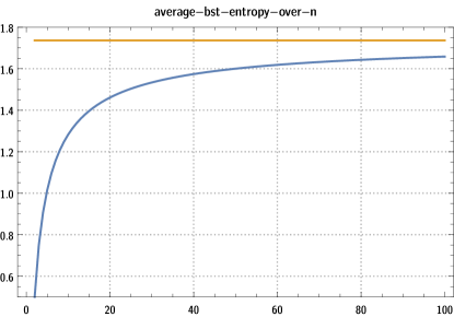
Figure 1. $H_{n}/n$ (blue) and its limit $\lim_{n\to\infty}H_{n}/n\approx 1.736$ (yellow) for $n\leq 100$.

5. An optimal encoding: subtree-size code

The formula for $\mathbb{P}[T_{n}=t]$, Equation (2), immediately suggests a route for an optimal encoding: We can rewrite the lower bound, $H_{n}$, as

$$H_{n} \mathchoice{\mathrel{\;\;{=}\;\;}}{\mathrel{=}}{\mathrel{=}}{\mathrel{=}}-\sum_{T\in\mathcal{T}_{n}}\mathbb{P}[T]\cdot\lg(\mathbb{P}[T])$$

$$\mathchoice{\mathrel{\;\;{=}\;\;}}{\mathrel{=}}{\mathrel{=}}{\mathrel{=}}\sum_{T\in\mathcal{T}_{n}}\mathbb{P}[T]\cdot\underbrace{\sum_{v\in t}\lg\bigl{(}\mathit{st}(v)\bigr{)}}_{\textstyle\mathcal{H}_{\mathit{st}(t)}}$$

$$\mathchoice{\mathrel{\;\;{=}\;\;}}{\mathrel{=}}{\mathrel{=}}{\mathrel{=}}\mathbb{E}[\mathcal{H}_{\mathit{st}}(T)].$$ (5)

That means, an encoding that spends $\mathcal{H}_{\mathit{st}}(t)$ bits to encode tree $t\in\mathcal{T}_{n}$ has optimal expected code length! In a slight abuse of the term, we will call the quantity $\mathcal{H}_{\mathit{st}}(t)=\sum_{v\in t}\lg\bigl{(}\mathit{st}(v)\bigr{)}$ the subtree-size entropy of a binary tree $t$.

Expressed for individual nodes, Equation (5) says we may spend $\lg s$ bits for a node whose subtree size is $s$. Now, what can we store in $\lg s$ bits for each node that uniquely describes the tree? One option is the size of each node’s left subtree. If a node $v$ has subtree size $\mathit{st}(v)=s$, then its left subtree has size $\mathit{ls}(v)=\mathit{st}(\mathit{left}(v))\in[0..s-1]$ (“left size”), a quantity with $s$ different values. Moreover, for random BSTs, each if these $s$ values is equally likely.

Figure 2. Example of the Cartesian tree $T$ for an array of 20 numbers. Each node shows the inorder number (in the node, coincides with the array index), its preorder index (above the node) and the sizes of left subtree and its total subtree (blue, below the node). We have $\mathcal{H}_{\mathit{st}}(T)\approx 28.74$, slightly below the expectation $H_{20}\approx 29.2209$. The arithmetic code for the preorder sequence of left tree sizes is 111011010111101011110101011111, i. e., 30 bits. This compares very favorably to a typical balanced parenthesis representation which would use $40$ bits.

The encoding of a tree $T$ stores $n$, the number of nodes followed by all left subtree sizes of the nodes in preorder, which we compress using arithmetic coding [27]. To encode $\mathit{ls}(v)$, we feed the arithmetic coder with the model that the next symbol is a number in $[0..\mathit{st}(v)-1]$ (all equally likely). Overall we then need $\mathcal{H}_{\mathit{st}}(T)+2$ bits to store $T$ when we know $n$. (Recall that arithmetic coding compresses to the entropy of the given input plus at most 2 bits of overhead.) Taking expectations over the tree $T$ to encode, we can thus store a binary tree with $n$ nodes using $H_{n}+O(\log n)\approx 1.736n+O(\log n)$ bits on average.

We can reconstruct the tree recursively from this code. Since we always know the subtree size, we know how many bins the next left tree size uses, and we know how many nodes we have to read recursively to reconstruct the left and right subtrees. Since arithmetic coding uses fractional numbers of bits for individual symbols (left tree sizes), decoding must always start at the beginning. This of course precludes any efficient operations on the encoding itself, so a refined approach is called for.

5.1. Bounding the worst case

Although optimal in the average case, the above encoding needs $\Theta(n\log n)$ bits in the worst case: in a degenerate tree (an $n$-path), the subtree sizes are $n,n-1,n-2,\ldots,1$ and hence the subtree-size entropy is $\sum_{i=1}^{n}\lg i\sim n\lg n$. For such trees, we are better off using one of the standard encodings using $2n+O(1)$ bits on any tree, for example Zak’s sequence (representing each node by a $1$ and each null pointer by a $0$). We therefore prefix our encoding with 1 extra bit to indicate the used encoding and then either proceed with the average-case optimal or the worst-case optimal encoding. That combines the best of both worlds with constant extra cost (in time and space). We can thus encode any tree $t\in\mathcal{T}_{n}$ in

$$2\lceil\lg n\rceil\mathchoice{\mathbin{\>{+}\>}}{\mathbin{+}}{\mathbin{+}}{\mathbin{+}}\min\bigl{\{}\mathcal{H}_{\mathit{st}}(t)+3,2n+2\bigr{\}}\text{ bits,}$$

where the first summand accounts for storing $n$ (in Elias code). Since we store $n$ alongside the tree shape, this encoding can be used to store any tree with maximal size $n$ in the given space.

The above encoding immediately generalizes to, and gives optimal space for, a more general family of distributions over tree shapes: We only need that the distribution of the size of the left subtree of a node $v$ depends only on the size of $v$’s subtree (but is conditionally independent of the shapes of $v$’s subtrees and the shape of the tree above $v$). In the case of random BSTs, this distribution is uniform (so our encoding is best possible), but in general, we can adapt the encoding of our trees to any family of left-size distributions, in particular to the empirical distributions found in any given tree. This yields better compression for skewed tree shapes.

6. Tree Covering

In this section, we review the tree-covering (TC) technique for succinct tree data structures. The idea of tree covering was introduced by Geary, Raman and Raman [11] (for ordinal trees) and later simplified by Farzan and Munro [6]; He, Munro and Rao [15] added further operations for ordinal trees and Davoodi et al. [4] designed inorder support. Tree covering has predominantly been used for ordinal trees, and it can be extended to support updates, but our presentation is geared towards succinctly storing static binary trees.

6.1. Trees, mini trees, micro trees

The main idea of TC is to partition the nodes of a tree into subsets that form contiguous subtrees. These subtrees are then (conceptually) contracted into a single node, and a second such grouping step is applied. We then represent the overall (binary) tree as a (binary) tree of mini trees, each of which is a (binary) tree of micro trees, each of which is a (binary) tree of actual nodes:

The number of nodes in micro trees is kept small enough so that an encoding of the local topology of each micro tree fits into less than one word, say $\frac{1}{2}\lg n$ bits. The number of (original) nodes in one mini tree is polylogarithmic (usually $\lg^{2}n$), so that the overall tree (the green level) has few enough nodes to fit a non-succinct (e. g., pointer-based) representation into $o(n)$ bits of space. The $O(n/\log^{2}n)$ mini trees can similarly be stored with pointers by restricting them to the polylogarithmic range inside a given mini tree. More generally, we can afford to store the overall tree (of mini trees, a. k. a. tier-1 macro tree) and the mini trees (of micro trees, a. k. a. tier-2 macro trees) using any representation that uses $O(n\log n)$ bits for an $n$-node tree.

For the micro trees, we use the so-called “Four Russian trick”: The type, i. e., the local topology, for each micro tree is stored in an array, and used as index into a large precomputed lookup table to answer any micro-tree-local queries. Since there are only $2^{\lg n/2}=\sqrt{n}$ different micro-tree types, this lookup table occupies $o(n)$ bits of space even with precomputed information for any pair of nodes.

6.2. Tree decomposition

We left open how to find a partition of the nodes into subtrees. A greedy bottom-up approach suffices to break a tree of $n$ nodes into $O(n/B)$ subtrees of $O(B)$ nodes each [11]. However, more carefully designed procedures yield additionally that any subtree has only few edges leading out of this subtree [6]. While originally formulated for ordinal trees, we note that on binary trees, the decomposition algorithm of Farzan and Munro [6] always creates a partition of the nodes, i. e., there are no subtrees sharing a common root:

Lemma 6.1 ([6, Theorem 1] for binary trees).

For any parameter $B\geq 1$, a binary tree with $n$ nodes can be decomposed, in linear time, into $\Theta(n/B)$ pairwise disjoint subtrees of $\leq 2B$ nodes each. Moreover, each of these subtrees has at most three connections to other subtrees:

• an edge from a parent subtree to the root of the subtree,

• an edge to another subtree in the left subtree of the root,

• an edge to another subtree in the right subtree of the root.

In particular, contracting subtrees into single nodes yields again a binary tree.

The decomposition scheme of Farzan and Munro additionally guarantees that (at least) one of the edges to child subtrees emanates from the root; we do not exploit this property in our data structure, though.

We found that it simplifies the presentation to assume that each subtree contains a copy of the root of its child subtrees, i. e., all subtree roots (except for the overall root) are present in two subtrees: once as root of the subtree and once as a leaf in the parent subtree. We refer to the copy in the parent as the portal of the (parent) subtree (to the child subtree). (An equivalent point of view is that we partition the edges of the tree and a subtree contains all nodes incident to those edges.) By Lemma 6.1, each subtree has at most one left portal and one right portal.

6.3. Node ids: $\tau$-names

For computations internal to the data structure, we represent nodes by “$\tau$-names”, i. e., by triples $(\tau_{1},\tau_{2},\tau_{3})$, where $\tau_{1}$ is the (preorder number of the) mini-tree, $\tau_{2}$ is the (mini-tree-local preorder number of the) micro tree and $\tau_{3}$ is the (micro-tree-local preorder number of the) node. Geary, Raman and Raman [11] show that the triple fits in $O(1)$ words and we can find a node’s $\tau$-name given its (global) preorder number, and vice versa, in constant time using additional data structures occupying $o(n)$ bits of space; we sketch these because they are typical examples of TC index data structures.

preorder $\mapsto$ $\tau$-name: $\mathit{nodeselect}_{\mathit{preorder}}$

We store $\tau_{1}$ and $\tau_{2}$ for all nodes in preorder in two piecewise-constant arrays. Since mini resp. micro trees are complete subtrees except for up to two subtrees that are missing, any tree traversal visits the nodes of one subtree in at most three contiguous ranges, so the above arrays change their values only $O(n/\log^{2}n)$ resp. $O(n/\log n)$ times and can thus be stored in $o(n)$ bits of space by Lemma 2.4. In a third piecewise-constant array, we store the $\tau_{3}$-value for the first node in the current micro-tree range; we obtain the $\tau_{3}$-value for any given node by adding the result of the runlen operation (Remark 2.6).

$\tau$-name $\mapsto$ preorder: $\mathit{noderank}_{\mathit{preorder}}$

The inverse mapping is more complicated in [11] since subtrees can have many child subtrees using their decomposition scheme. With the stronger properties from Lemma 6.1, computing a node’s preorder is substantially simpler. We store for each mini resp. micro tree the following information:

• the preorder index of the root
  (in micro trees: local to the containing mini tree),

• the (subtree-local) preorder index of the left and right portals
  (in mini trees: these indices are w. r. t. actual nodes, not micro trees),

• the subtree size of the portal’s subtrees
  (in micro trees: local to the containing mini tree).

For mini trees, these numbers fit in $O(\log n)$ bits each and can thus be stored for all $O(n/\log^{2}n)$ mini trees in $o(n)$ space. For micro trees, we store information relative to the surrounding mini tree, so the numbers fit in $O(\log\log n$) bits each, again yielding $o(n)$ extra space overall.

To compute the preorder index for node $v$ with $\tau$-name $(\tau_{1},\tau_{2},\tau_{3})$, we start with the (mini-tree-local) preorder index of $\tau_{2}$’s root within $\tau_{1}$ and we add the subtree size of $\tau_{2}$’s left (right) portal if $\tau_{3}$ is larger than the left (right) portal’s micro-tree-local preorder index. The result is the preorder index $\tau_{3}^{\prime}$ of $v$ within $\tau_{1}$ (in terms of nodes, not in terms of micro trees). Applying the same computation, but using $\tau_{1}$’s portal information and starting with $\tau_{3}^{\prime}$, we obtain $v$’s global preorder index.

6.4. Lowest common ancestors

He, Munro and Rao [15] use known $O(n\log n)$-bit-space representations of ordinal trees that support constant-time lowest-common-ancestor queries to represent the tier-1 and tier-2 macro trees, and they give a (somewhat intricate) $O(1)$-time algorithm to compute lca based on these representations.

A conceptually simpler option is to use a $O(n)$-bit data structure for (static, ordinal) trees that supports lca queries by preorder indices, e. g., the one of Navarro and Sadakane [23]. Note that for lca queries and preorder numbers, the distinction in binary trees between unary nodes with only a left resp. only a right child is irrelevant. We construct the tree $T_{B}$ of all micro-tree roots by contracting micro trees into single nodes, (ignoring the mini-tree level), and store $T_{B}$ using the compact ordinal-tree data structure.

Using similar data structures as for $\mathit{noderank}_{\mathit{preorder}}$, we can compute the preorder number of a micro-tree root in the micro-tree-root tree $T_{B}$, denoted by $\mathit{noderank}_{\mathit{microRoot}}(\tau_{1},\tau_{2})$. The inverse operation, $\mathit{nodeselect}_{\mathit{microRoot}}$, is similar to $\mathit{nodeselect}_{\mathit{preorder}}$.

To find the LCA of two nodes $u$ and $v$ in the tree, we first find $k_{u}=\mathit{noderank}_{\mathit{microRoot}}(u)$ and $k_{v}=\mathit{noderank}_{\mathit{microRoot}}(v)$. If $k_{u}=k_{v}$, both nodes are in the same micro tree and so is their LCA, so we use the (micro-tree-local) lookup table to find the (precomputed) LCA.

Otherwise, when $k_{u}\neq k_{v}$, we determine $k=\mathit{lca}(T_{B},k_{u},k_{v})$, the LCA of the micro-tree roots in $T_{B}$. If $k_{u}\neq k\neq k_{v}$, then the paths from $k_{u}$ and $k_{v}$ first meet at micro-tree root $k$ and we return $\mathit{lca}(u,v)=\mathit{nodeselect}_{\mathit{microRoot}}(k)$.

The remaining case is that the LCA is one of $k_{u}$ or $k_{v}$; w. l. o. g. say $k=k_{u}$. This means that the micro-tree root $r=\mathit{nodeselect}_{\mathit{microRoot}}(k_{u})$ of $u$’s micro-tree root is an ancestor of $v$. Since $v$ is not in $r$’s micro tree, but in $r$’s subtree, it must be in the subtree of one of the portals. We find the right one by selecting the portal $p$ that fulfills $p=\mathit{lca}(T_{B},p,v)$. (If $T_{B}$ supports ancestor queries more efficiently, we can also ask whether $p$ is an ancestor of $v$.) Finally, as in the intra-micro-tree case, we find the lca of $u$ and $p$ within the micro tree.

6.5. Inorder rank and select

Davoodi et al. [4] describe $o(n)$ bit data structures that allow to map preorder to inorder and vice versa. For computing the inorder of a node $v$, they use the equation $\mathit{inorder}(v)=\mathit{preorder}(v)+\mathit{ls}(v)-\mathit{rightdepth}(v)$, where $\mathit{rightdepth}(v)$ is the the number of right-edges on the path from the root to $v$, i. e., the depth where only following right-child pointers counts. Storing the global right depth of each mini-tree root, the mini-tree-local right depth of each micro-tree root and micro-tree-local right-depth info in the lookup table, we can obtain the right-depth of any node by adding up these three quantities.

Instead of directly mapping from inorder to preorder (as done in [4]), we can adapt the above strategy for mapping inorder to $\tau$-name. Storing $\tau_{1}$ and $\tau_{2}$ for all nodes in inorder works the same as above. We cannot store $\tau_{3}$ directly in a piecewise constant array (it changes to often), but we can store the micro-tree-local inorder index, $\tau_{3}^{\textrm{in}}$. Finally, we use the lookup table to translate $\tau_{3}^{\textrm{in}}$ to $\tau_{3}$.

7. Entropy trees

The dominating contribution (in terms of space) in TC comes from the array of micro-tree types. All other data structures – for storing overall tree and mini trees, as well as the various index data structures to support queries – fit in $o(n)$ bits of space. Encoding micro trees using one of the $2n$-bit encodings for $\mathcal{T}_{n}$ (e. g., BP, DFUDS, or Zaks’ sequence), the combined space usage of the types of all micro trees is $2n+o(n)$ bits.

The micro-tree types are solely used as an index for the lookup table; how exactly the tree topology is encoded is immaterial. It is therefore possible to replace the fixed-length encoding by one that adapts to the actual input. Using variable-cell arrays (Lemma 2.2), the dominant space is the sum of the lengths of the micro-tree types.

Davoodi et al. [4] used the “ultra-succinct” encoding proposed by Jansson, Sadakane and Sung [18] for micro trees to obtain a data structure that adapts to the entropy of the node-degree distribution. This approach is inherently limited to non-optimal compression since it only depends on the local order of a fixed number of values in the input array. Using our new encoding for binary tree we can overcome this limitation.

Combining the tree-covering data structure for binary trees described in Section 6 with the (length bounded) subtree-size code for binary trees from Section 5 yields the following result.

Theorem 7.1 (Entropy trees).

Let $t\in\mathcal{T}_{n}$ be a (static) binary tree on $n$ nodes. There is a data structure that occupies $\min\{\mathcal{H}_{\mathit{st}}(t),2n\}+o(n)$ bits of space and supports the following operations in $O(1)$ time:

• find the node with given pre- or inorder index,

• find the pre- and inorder index of a given node,

• compute the lca of two given nodes.

Proof 7.2.

The correctness of operations and size of supporting data structures directly following from the previous work on tree covering (see Section 6) and the discussion above. It remains to bound the sum of code lengths of micro-tree types. Let $\mu_{1},\ldots,\mu_{\ell}$ denote the micro trees resulting from the tree decomposition. We have

$$\sum_{i=1}^{\ell}|\mathit{type}(\mu_{i})| \mathchoice{\mathrel{\;\;{\leq}\;\;}}{\mathrel{\leq}}{\mathrel{\leq}}{\mathrel{\leq}}\sum_{i=1}^{\ell}\sum_{v\in\mu_{i}}\Bigl{(}\mathit{st}_{\mu_{i}}(v)+2\Bigr{)}$$

$$\mathchoice{\mathrel{\;\;{\leq}\;\;}}{\mathrel{\leq}}{\mathrel{\leq}}{\mathrel{\leq}}\sum_{i=1}^{\ell}\sum_{v\in\mu_{i}}\mathit{st}_{t}(v)\mathchoice{\mathbin{\;\;{+}\;\;}}{\mathbin{+}}{\mathbin{+}}{\mathbin{+}}O\biggl{(}\frac{n}{\log n}\biggr{)}$$

$$\mathchoice{\mathrel{\;\;{\leq}\;\;}}{\mathrel{\leq}}{\mathrel{\leq}}{\mathrel{\leq}}\sum_{v\in t}\mathit{st}_{t}(v)\mathchoice{\mathbin{\;\;{+}\;\;}}{\mathbin{+}}{\mathbin{+}}{\mathbin{+}}O\biggl{(}\frac{n}{\log n}\biggr{)}$$

$$\mathchoice{\mathrel{\;\;{=}\;\;}}{\mathrel{=}}{\mathrel{=}}{\mathrel{=}}\mathcal{H}_{\mathit{st}}(t)\mathchoice{\mathbin{\;\;{+}\;\;}}{\mathbin{+}}{\mathbin{+}}{\mathbin{+}}O\biggl{(}\frac{n}{\log n}\biggr{)}.$$

Moreover, $|\mathit{type}(\mu_{i})|\leq 2|\mu_{i}|+O(1)$, so also $\sum_{i=1}^{\ell}|\mathit{type}(\mu_{i})|\leq 2n+O\bigl{(}\frac{n}{\log n}\bigr{)}$.

By using this data structure on the Cartesian tree of an array, we obtain a compressed RMQ data structure.

Corollary 7.3 (Average-case optimal succinct RMQ).

There is a data structure that supports (static) range-minimum queries on an array $A$ of $n$ (distinct) numbers in $O(1)$ worst-case time and which occupies $H_{n}+o(n)\approx 1.736n+o(n)$ bits of space on average over all possible permutations of the elements in $A$. The worst case space usage is $2n+o(n)$ bits.

Further operations

Since micro-tree types are only used for the lookup table, all previously described index data structures for other operations are not affected by swapping out the micro-tree encoding. Entropy trees can thus support the full range of (cardinal-tree) operations listed in [6, Table 2].

8. Hyper-succinct trees

The subtree-size code yields optimal compression for random BSTs, but is not a good choice for certain other shape distributions. However, we obtain instance-optimal compression by yet another encoding for micro trees: By treating each occurring micro-tree type as a single symbol and counting how often it occurs when storing a given tree $t$, we can compute a (length-bounded) Huffman code for the micro-tree types. We call the resulting tree-covering data structure “hyper succinct” since it yields better compression than ultra-succinct trees. Indeed, it follows from the optimality of Huffman codes that no other tree-covering-based data structure can use less space.

It is, however, quite unclear how good the compression for a given tree is; note in particular that the set of micro trees is a mixture of subtrees at the fringe of $t$ and subtrees from the “middle” of $t$ where one or two large subtrees have been pruned away. How repetitive this set of shapes is will depend not only on $t$, but also on the tree-decomposition algorithm and the size of micro trees.

References

- [1] http://github.com/ot/succinct.
- [2] Jérémy Barbay, Johannes Fischer, and Gonzalo Navarro. LRM-trees: Compressed indices, adaptive sorting, and compressed permutations. Theoretical Computer Science, 459:26–41, November 2012. doi:10.1016/j.tcs.2012.08.010.
- [3] Niklas Baumstark, Simon Gog, Tobias Heuer, and Julian Labeit. Practical range minimum queries revisited. In Costas S. Iliopoulos, Solon P. Pissis, Simon J. Puglisi, and Rajeev Raman, editors, International Symposium on Experimental Algorithms (SEA), volume 75 of LIPIcs, pages 12:1–12:16. Schloss Dagstuhl–Leibniz-Zentrum fuer Informatik, 2017. doi:10.4230/LIPIcs.SEA.2017.12.
- [4] Pooya Davoodi, Gonzalo Navarro, Rajeev Raman, and Srinivasa Rao Satti. Encoding range minima and range top-2 queries. Philosophical Transactions of the Royal Society A: Mathematical, Physical and Engineering Sciences, 372(2016):20130131–20130131, apr 2014. doi:10.1098/rsta.2013.0131.
- [5] Pooya Davoodi, Rajeev Raman, and Srinivasa Rao Satti. On succinct representations of binary trees. Mathematics in Computer Science, 11(2):177–189, March 2017. doi:10.1007/s11786-017-0294-4.
- [6] Arash Farzan and J. Ian Munro. A uniform paradigm to succinctly encode various families of trees. Algorithmica, 68(1):16–40, June 2012. doi:10.1007/s00453-012-9664-0.
- [7] Héctor Ferrada and Gonzalo Navarro. Improved range minimum queries. Journal of Discrete Algorithms, 43:72–80, mar 2017. doi:10.1016/j.jda.2016.09.002.
- [8] Johannes Fischer. Data Structures for Efficient String Algorithms. Dissertation (Ph. D. thesis), 2007.
- [9] Johannes Fischer and Volker Heun. Space-efficient preprocessing schemes for range minimum queries on static arrays. SIAM Journal on Computing, 40(2):465–492, January 2011. doi:10.1137/090779759.
- [10] Harold N. Gabow, Jon Louis Bentley, and Robert E. Tarjan. Scaling and related techniques for geometry problems. In STOC 1984. ACM Press, 1984. doi:10.1145/800057.808675.
- [11] Richard F. Geary, Rajeev Raman, and Venkatesh Raman. Succinct ordinal trees with level-ancestor queries. ACM Transactions on Algorithms, 2(4):510–534, October 2006. doi:10.1145/1198513.1198516.
- [12] Simon Gog, Timo Beller, Alistair Moffat, and Matthias Petri. From theory to practice: Plug and play with succinct data structures. In International Symposium on Experimental Algorithms (SEA), pages 326–337, 2014. doi:10.1007/978-3-319-07959-2_28.
- [13] Mordecai Golin, John Iacono, Danny Krizanc, Rajeev Raman, Srinivasa Rao Satti, and Sunil Shende. Encoding 2d range maximum queries. Theoretical Computer Science, 609:316–327, January 2016. doi:10.1016/j.tcs.2015.10.012.
- [14] Dan Gusfield. Algorithms on Strings, Trees and Sequences. Cambridge University Press, 1997.
- [15] Meng He, J. Ian Munro, and Srinivasa Satti Rao. Succinct ordinal trees based on tree covering. ACM Transactions on Algorithms, 8(4):1–32, September 2012. doi:10.1145/2344422.2344432.
- [16] Hsien-Kuei Hwang and Ralph Neininger. Phase change of limit laws in the quicksort recurrence under varying toll functions. SIAM Journal on Computing, 31(6):1687–1722, jan 2002. doi:10.1137/s009753970138390x.
- [17] Philippe Jacquet and Wojciech Szpankowski. Analytic Pattern Matching. Cambridge University Press, 2015.
- [18] Jesper Jansson, Kunihiko Sadakane, and Wing-Kin Sung. Ultra-succinct representation of ordered trees with applications. Journal of Computer and System Sciences, 78(2):619–631, March 2012. doi:10.1016/j.jcss.2011.09.002.
- [19] Seungbum Jo, Shay Mozes, and Oren Weimann. Compressed range minimum queries. In Navarro G. Cuadros-Vargas E. Gagie T., Moffat A., editor, International Symposium on String Processing and Information Retrieval (SPIRE), pages 206–217. Springer, 2018. doi:10.1007/978-3-030-00479-8_17.
- [20] John C. Kieffer, En-Hui Yang, and Wojciech Szpankowski. Structural complexity of random binary trees. In 2009 IEEE International Symposium on Information Theory. IEEE, jun 2009. doi:10.1109/isit.2009.5205704.
- [21] Abram Magner, Krzysztof Turowski, and Wojciech Szpankowski. Lossless compression of binary trees with correlated vertex names. IEEE Transactions on Information Theory, 64(9):6070–6080, sep 2018. doi:10.1109/tit.2018.2851224.
- [22] Gonzalo Navarro. Compact Data Structures – A practical approach. Cambridge University Press, 2016.
- [23] Gonzalo Navarro and Kunihiko Sadakane. Fully functional static and dynamic succinct trees. ACM Transactions on Algorithms, 10(3):1–39, may 2014. doi:10.1145/2601073.
- [24] Rajeev Raman, Venkatesh Raman, and Srinivasa Rao Satti. Succinct indexable dictionaries with applications to encoding k-ary trees, prefix sums and multisets. ACM Transactions on Algorithms, 3(4):43–es, nov 2007. doi:10.1145/1290672.1290680.
- [25] Rajeev Raman and S. Srinivasa Rao. Succinct representations of ordinal trees. In Raman V.-Viola A. Brodnik A., López-Ortiz A., editor, Space-Efficient Data Structures, Streams, and Algorithms, volume 8066 of LNCS, pages 319–332. Springer, 2013. doi:10.1007/978-3-642-40273-9_20.
- [26] Jean Vuillemin. A unifying look at data structures. Communications of the ACM, 23(4):229–239, April 1980. doi:10.1145/358841.358852.
- [27] Ian H. Witten, Radford M. Neal, and John G. Cleary. Arithmetic coding for data compression. Communications of the ACM, 30(6):520–540, jun 1987. doi:10.1145/214762.214771.