The Expansion of the Forward Shock of 1E 0102.2-7219 in X-rays

Abstract

We measure the expansion of the forward shock of the Small Magellanic Cloud supernova remnant 1E 0102.2-7219 in X-rays using Chandra X-Ray Observatory on-axis Advanced CCD Imaging Spectrometer (ACIS) observations from 1999–2016. We estimate an expansion rate of $0.025\%\pm 0.006\%~{}\mathrm{yr}^{-1}$ and a blast-wave velocity of $1.61\pm 0.37\times 10^{3}~{}\mathrm{km~{}s}^{-1}$. Assuming partial electron-ion equilibration via Coulomb collisions and cooling due to adiabatic expansion, this velocity implies a postshock electron temperature of $0.84\pm 0.20~{}\mathrm{keV}$ which is consistent with the estimate of $0.68\pm 0.05~{}\mathrm{keV}$ based on the X-ray spectral analysis. We combine the expansion rate with the blast wave and reverse shock radii to generate a grid of one-dimensional models for a range of ejecta masses ($2-6\,\mbox{$\mathrm{M}_{\sun}$}$) to constrain the explosion energy, age, circumstellar density, swept-up mass, and unshocked-ejecta mass. We find acceptable solutions for a constant density ambient medium and for an $r^{-2}$ power-law profile (appropriate for a constant progenitor stellar wind). For the constant density case, we find an age of $\sim\,1700~{}\mathrm{yr}$, explosion energies $0.87-2.61\times 10^{51}~{}\mathrm{erg}$, ambient densities $0.85-2.54~{}\mathrm{amu\,cm}^{-3}$, swept-up masses $22-66\,\mbox{$\mathrm{M}_{\sun}$}$, and unshocked-ejecta masses $0.05-0.16\,\mbox{$\mathrm{M}_{\sun}$}$. For the power-law density profile, we find an age of $\sim 2600~{}\mathrm{yr}$, explosion energies $0.34-1.02\times 10^{51}~{}\mathrm{erg}$, densities $0.22-0.66~{}\mathrm{amu\,cm}^{-3}$ at the blast wave, swept-up masses $17-52\,\mbox{$\mathrm{M}_{\sun}$}$, and unshocked-ejecta masses $0.06-0.18\,\mbox{$\mathrm{M}_{\sun}$}$. Assuming the true explosion energy was $0.5-1.5\times 10^{51}~{}\mathrm{erg}$, ejecta masses $2-3.5\,\mbox{$\mathrm{M}_{\sun}$}$ are favored for the constant density case and $3-6\,\mbox{$\mathrm{M}_{\sun}$}$ for the power-law case. The unshocked-ejecta mass estimates are comparable to Fe masses expected in core-collapse supernovae with progenitor mass $15.0-40.0\,\mbox{$\mathrm{M}_{\sun}$}$, offering a possible explanation for the lack of Fe emission observed in X-rays.

1 Introduction

The supernova remnant (SNR) 1E 0102.2-7219 (hereafter E0102) is the X-ray brightest SNR in the Small Magellanic Cloud (SMC) with a luminosity of $1.1\times 10^{37}$ $\mathrm{erg}\,\mathrm{s}^{-1}$ in the 0.5-2.0 keV band. E0102 was discovered by Seward & Mitchell (1981) with the Einstein Observatory. It was classified as an “O-rich” SNR based on the optical spectra acquired soon after the X-ray discovery by Dopita et al. (1981) and confirmed by follow-up observations of the complex optical emission in [O III] and [O II] (Tuohy & Dopita, 1983). Blair et al. (1989) presented the first UV spectra of E0102 and argued for a progenitor mass between 15 and 25 $\mathrm{M}_{\sun}$ based on the derived O, Ne, and Mg abundances. Blair et al. (2000) refined this argument with Wide Field and Planetary Camera 2 (WFPC2) and Faint Object Spectrograph data from Hubble Space Telescope (HST) to suggest that the precursor was a Wolf-Rayet star of between 25 and 35 $\mathrm{M}_{\sun}$ with a large O mantle that produced a Type Ib supernova. The optical morphology shows a complicated, filamentary structure first seen by Tuohy & Dopita (1983) and then seen in more detail in the HST WFPC2 [O III] $\lambda=5007$ (F502N) image in Blair et al. (2000). Finkelstein et al. (2006) confirm this complicated structure with images from several filters from the Advanced Camera for Surveys (ACS) on HST. In contrast, the X-ray morphology observed with the Chandra X-ray Observatory (Chandra) is considerably simpler than that observed in the optical. Gaetz et al. (2000) presented high resolution images from Chandra that allow the blast wave emission to be separated from the ejecta emission (see Figure 1). There is a good correlation between the optical and X-ray emission for some of the filaments as shown in the right panel of Figure 1 but for other filaments there is little or no correlation. The outer blastwave is well-defined in the X-rays but is notably absent in the optical.

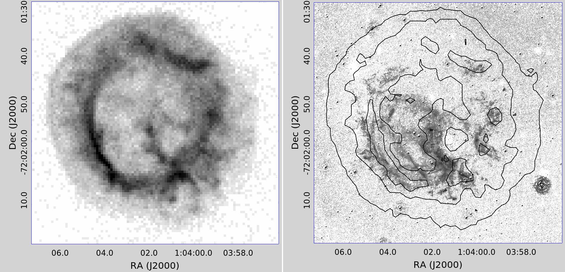
Figure 1: X-ray and optical emission of E0102. Left panel: Chandra data for ObsID 1423 (binned to 1 ACIS sky pixel, 0.4-2.0 keV), with a sqrt color stretch. Right panel: HST ACS data (continuum subtracted) with a logarithmic color stretch. X-ray contours are overplotted on the optical image.

In an early Chandra study of the first ACIS images of E0102 (ObsID 1231), Hughes et al. (2000, hereafter HRD00) investigated the post-shock partition of energy among electrons, ions, and a putative population of relativitisic particles, i.e., cosmic rays, at the forward shock of the remnant. The forward shock was cleanly resolved in the ACIS data and its spectrum was extracted; using nonequilibrium ionization (NEI) thermal emission models, HRD00 determined the post-shock electron temperature to be 0.4-1 keV with a significant component of the acceptable range due to model uncertainty. The proper motion of the entire SNR (assumed to be both radially and azimuthally uniform) was determined by comparing the Chandra ACIS image to archival Einstein and Röntgensatellite (ROSAT) High Resolution Imager images taken $\sim$8 and $\sim$20 years earlier, respectively. These earlier images had 50% encircled energy radii of $4^{\prime\prime}$, more than 10 times larger than that of the Chandra ACIS image. The fractional expansion rate of the entire remnant was $0.100\%\pm 0.025\%$ yr^-1, which, when extrapolated to the location of the forward shock, implied a shock speed of $\sim$6000 km s^-1. Converting the shock speed to an electron temperature required accounting for the uncertain amount of anomalous heating at the shock front followed by energy exchange through Coulomb collisions between the electron and ion thermal populations, as well as estimating the amount of adiabatic decompression in the measured postshock region. After these calculations, HRD00 found the minimum expected electron temperature to be $\sim$2.5 keV, significantly higher than the measured temperature value, leading to the suggestion that some of the forward shock energy in E0102 went into generating cosmic rays.

In this paper we make the first direct measurement of the forward shock speed in E0102 using multiple epochs of Chandra observations. We use Chandra’s exquisite angular resolution to separate the forward shock from the interior emission of the remnant. This allows us to measure the expansion of the forward shock alone without any confusion from other parts of the remnant that may have different velocities. We closely follow the approach of HRD00 while updating the electron temperature measurements, improving the shock electron temperature model, and constraining the age, ambient medium density, ejected mass, and other dynamical quantities from an analytical shock model. Our paper is structured as follows. In §2 we describe the Chandra ACIS observations of E0102 and in §3 we present our full analysis including measuring the proper motion of the forward shock and the radial locations of the forward and reverse shocks. §4 describes our one-dimensional analytical shock model and gives results on the dynamical state of the SNR. Also in Section §4 we determine the post-shock electron temperature directly from spectral modeling and also by calculation from the forward shock speed. §5 concludes. Throughout this paper we assume the distance to the SMC is 60.6 kpc (Hilditch et al., 2005). Error bars in plots and uncertainties on numerical values are quoted at the 1$\sigma$ confidence level unless otherwise stated.

2 Chandra Observations of E0102

As a calibration source for Chandra, E0102 has been observed every year from 1999 to 2018. An overview of Chandra including the imaging capabilities of the High Resolution Mirror Assembly (HRMA) is given in (Weisskopf et al., 2000, 2002). We utilize data from the Advanced CCD Imaging Spectrometer (ACIS) instrument which is described in detail in  Garmire et al. (1992); Bautz et al. (1998); Garmire et al. (2003). The ACIS instrument contains two arrays of charge-coupled devices (CCDs), an imaging array called ACIS-I and a spectroscopy array called ACIS-S. The central CCD of the ACIS-S array (called S3) is a backside-illuminated (BI) CCD which has superior low energy quantum efficiency compared to the frontside-illuminated (FI) CCDs in ACIS. We select 12 ACIS-S3 observations, with exposure times ranging from $\sim$ 7.6-19.7 ks (see Table 1), that had the center of the remnant positioned within $1^{\prime}$ of the on-axis aim point to provide the optimal imaging performance with Chandra. We exclude from our analysis the off-axis observations of E0102 with sub-optimal imaging and the on-axis observations after 2017 as the correction for the additional absorption caused by the contamination layer on the ACIS filters has become less certain after 2017 (Plucinsky et al., 2018). Each observation is reprocessed to generate a new level=2 event list, using CIAO version 4.8 and CALDB 4.7.2, by the CIAO tool chandra_repro, with the option pix_adj set to the default, such that the Energy Dependent Sub-pixel Event Reconstruction (EDSER) algorithm is applied. This enables sub-pixel resolution in imaging data analysis (Li et al., 2004) by using the distribution of charge amongst the pixels within a $3\times 3$ pixel detection island to estimate a better position for where the X-ray landed in the central pixel.

E0102 was observed in ACIS subarray mode starting in 2003 to achieve a shorter frametime which reduces photon “pileup”. Photon pileup is the condition in which two or more photons interact with the CCD within the event detection cell (typically $3\times 3$ pixels for ACIS) within a single frame, resulting in an incorrect energy and perhaps position for the events. The brightest parts of E0102 (for example the white and red regions in Figure 2 bottom left panel) are bright enough to produce significant pileup which depresses the observed count rate and shifts the distribution of observed energies to higher energies. The pileup level can exceed 5% as shown for a fullframe observation with a 3.2 s frametime (bottom left panel of Figure 2). Pileup can be significantly reduced if the frametime is decreased to 0.8s as it was in the 2003 and later observations. The outer blastwave has a low enough surface brightness that pileup is negligible even in the earliest observations in fullframe mode. Another factor which reduces pileup in the later E0102 observations is the accumulation of a contamination layer on the ACIS optical blocking filters (OBF) (see Plucinsky et al., 2003, 2016). The ACIS contamination layer produces a highly energy-dependent absorption with low energy photons around 0.5 keV suffering high absorption while higher energy photons around 1.5 keV and up suffering little absorption. By the time of the observation in 2016, the combination of the shorter frametime and the contamination layer resulted in the bright parts of the ring having negligible pileup.

For our analysis, we focus primarily on the outer blastwave which is free from the effects of pileup even for the fullfame mode observations. We make use of only two fullframe mode observations, one from 1999 (ObsID 1423) as the first observation in a sequence to measure the position of the blastwave and the second from 2006 (ObsID 6766). We include 6766 as a check on our registration method discussed in §3.3 as it is the latest fullframe observation on S3. The remaining observations in our analysis are in subarray mode (see Table 1) and in fact all of the observations after 2006 are in subarray mode.

Table 1: Observation List

ObsID	Start Date	Exposure	Time difference	Full-frame
		(ks)	(yr)
1423	1999 Nov 01	18.92	00.00	Y
3545	2003 Jun 06	07.86	03.60	N
6765	2006 Mar 19	07.64	06.38	N
6766	2006 Jun 06	19.70	06.59	Y
9694	2008 Feb 07	19.20	08.27	N
11957	2009 Dec 30	18.45	10.17	N
13093	2011 Feb 01	19.05	11.26	N
14258	2012 Jan 12	19.05	12.20	N
15467	2013 Jan 28	19.08	13.25	N
16589	2014 Mar 27	09.57	14.41	N
17380	2015 Feb 28	17.65	15.34	N
18418	2016 Mar 15	14.33	16.38	N

3 Analysis

The objective of our analysis is to measure the change in the position of the blast wave of the SNR as a function of time to determine the velocity of the shock. Our approach is summarized here and described in detail in the following sections. We first construct a reference image (called the “model”) from an observation early in the Chandra mission that had a relatively high count rate to provide good statistics. We construct images from the later observations (called the “comparison data”) using the same processing as the reference image. We correct the model image for the change in quantum efficiency (QE) as a function of time and energy given the time difference between the observation date of the model image and that of the comparison data. We register the images using the bright, central feature in E0102. We extract radial profiles in 16 directions and fit the profiles with a model of the shock emission smoothed by the angular resolution of the combined HRMA and ACIS system. We measure the shifts between the model and comparison data profiles to derive offsets in the 16 directions. We then fit the offsets as a function of position angle with a sinusoidal function to account for any remaining error in the registration. From this fit, we determine the best fitted value of the average expansion for each combination of comparison data and model image. We then repeat this exercise for the subarray observations in Table 1 using ObsID 1423 for the reference image to determine the average expansion as a function of time.

3.1 Image Generation

The images were created by using the standard CIAO tool dmcopy to bin the events into $0.246\arcsec\times 0.246\arcsec$ sky pixels in the $0.5-2.0$ keV energy range. The EDSER algorithm had already been applied to the events list before the images were created. The imaging improvement results from dither moving the pixel center across the image combined with the slight imaging improvement from EDSER. The pixel size of $0.246\arcsec\times 0.246\arcsec$ was selected to optimize the imaging information of the HRMA and ACIS combination while providing sufficient statistics in a single pixel. The energy range of $0.5-2.0$ keV was selected to optimize the signal from the SNR compared to the detector and sky background components.

3.1.1 Model Image Generation

ObsID 1423 was used to construct the model image of E0102 since the exposure time of 18.9 ks was relatively long compared to other observations of E0102 and the observation was executed on 1999 November 01 when the ACIS contamination layer was relatively thin. Because the quantum efficiency (QE) and exposure time changed between ObsID 1423 and later observations, the counts in each bin of the model image need to be weighted by a factor to account for the QE and exposure time differences. The weighting factor was applied to each event in the events list of ObsID 1423 and a new image of the weighted events was created using dmcopy. The weights were calculated as $q_{2}t_{2}/q_{1}t_{1}$ where $q_{1}$ is the QE at the energy of the event for the date of ObsID 1423, $q_{2}$ is the QE for the date of the comparison observation, $t_{1}$ is the exposure time of ObsID 1423, and $t_{2}$ is the exposure time of the comparison observation. To determine the QE of an event at a given energy and a given point in time, we used the CIAO tool eff2evt by setting the option detsubsysmod to the start time of the observation. We obtained $q_{1}$ by setting detsubsysmod to the start time of ObsID 1423, and $q_{2}$ by setting it to the start time of comparison observation. The model image was smoothed with a $\sigma=0.492\arcsec$ Gaussian. Figure 2 displays the image from ObsID 1423 in the $0.5-2.0$ keV band in the top panel. The lower left panel shows the pileup percentage as calculated by the CIAO tool pileup_map for ObsID 1423, and the bottom right panel shows the pileup percentage for a subarray mode observation ObsID 3545 (note that the color scales for the bottom left and bottom right panels are different). Since ObsID 1423 used a frametime of 3.2 s and the contamination layer was relatively thin in 1999, the bright ring of E0102 has significant pileup (maximum value is $\sim 10\%$). However, the outer blastwave is essentially free of pileup given that it is much fainter than the bright ring.

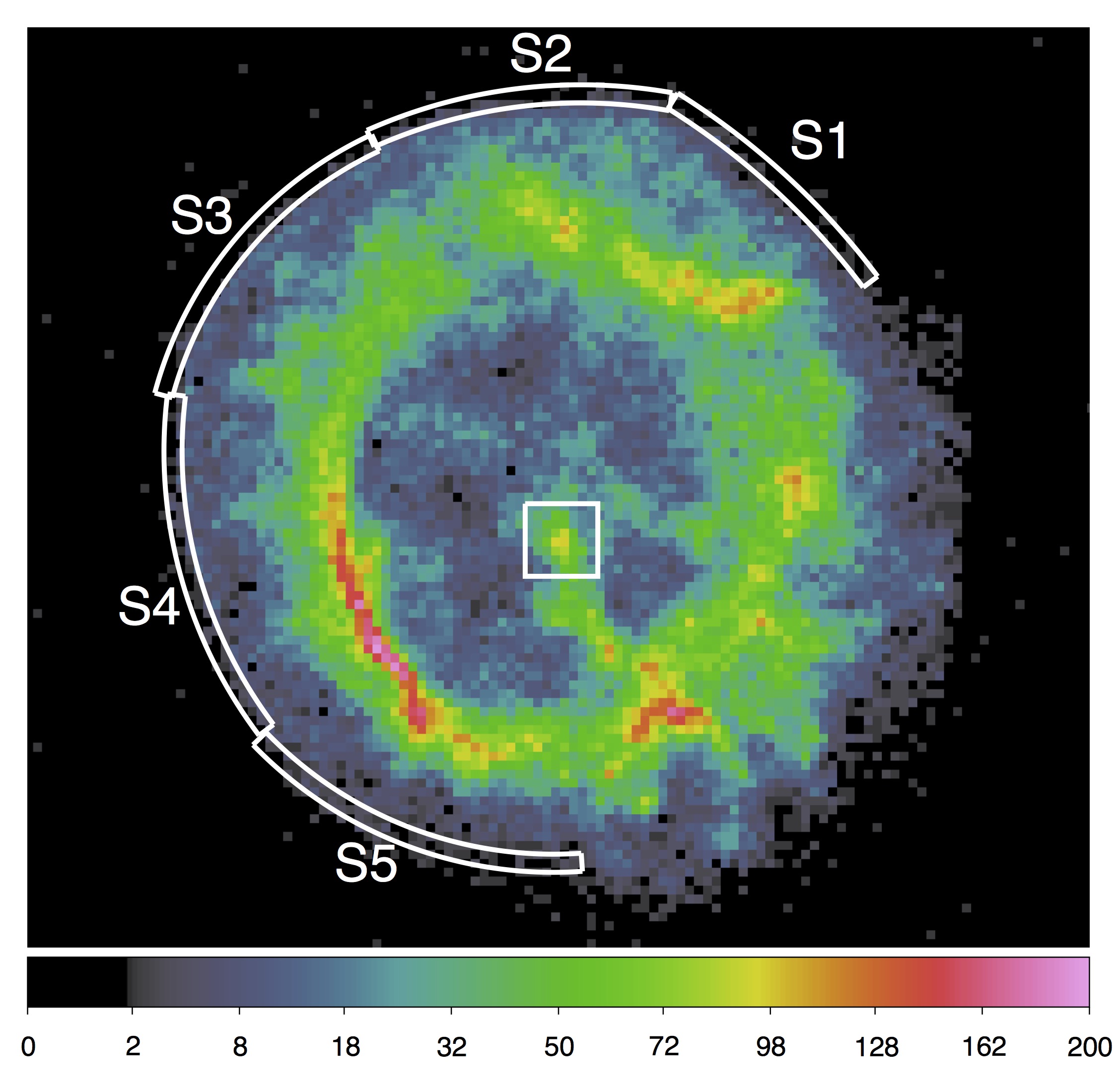
Figure 2: Top Left: Image from ObsID 1423 in the 0.5–2.0 keV band. The units for the image and the colorbar are counts. The annular regions ($1.0\arcsec$ width) show the spectral extraction regions for the blastwave spectrum and the box region in the center shows the region used for registration. Bottom Left: ObsID 1423 pileup map (early full-frame observation). The units for the image and color bar are counts/frame. A value of 0.1/0.2 counts/frame corresponds to $\sim 5/10\%$ pileup. Bottom Right: pileup map of ObsID 3545 in 2003, a subarray observation with a shorter frametime. The units for the image and color bar are counts/frame. Pileup is less than $5\%$ even for the brightest regions in ObsID 3545. Note that the color scale ranges for the bottom panels are different.

3.2 Comparison Data Image Generation

The subarray observations in Table 1 were used to construct the comparison data images. Figure 2 (bottom right panel) shows the image from ObsID 3545 with a 1.1 s frametime from 2003 when the contamination layer was thicker than it was for ObsID 1423. Since the frametime is shorter than it was for ObsID 1423 and the rate incident on the detector is reduced due to the contamination layer, the pileup is significantly reduced with no pixel having more than 5% pileup. Note that the color scale is different for this image than for the pileup map for ObsID 1423. All subarray observations listed in Table 1 observed after ObsID 3545 use a frametime of 0.8 s, which reduces pileup further. The comparison images have no corrections applied to them and are treated as the “data”. As discussed in the previous section, the image from ObsID 1423 is treated as the “model” and hence the QE and exposure time corrections are applied to that image before comparison with the later data sets.

3.3 Image Registration

Since the observations of E0102 after 2006 were acquired in subarray mode, there are no point sources in the field of view which we can use for registration. To take advantage of the nearly 17 year baseline of observations of E0102, we used the central bright feature defined by a $4^{\prime\prime}$ by $4^{\prime\prime}$ box region (shown in Figure 2, top panel), centered on $\alpha_{J2000}=01^{h}04^{m}2.1^{s}$, $\delta_{J2000}=-72^{\circ}1^{\prime}55.6^{\prime\prime}$ to register the observations to ObsID 1423. This feature, which is near the expansion center of the optical filaments given by Finkelstein et al. (2006, hereafter F06), is located close to some of the bright optical filaments shown in Figure 1. According to measurements by Eriksen et al. (2001) and Vogt & Dopita (2010), this region contains blue-shifted material with a maximum velocity ranging from 2100$\;\mathrm{km}\,\mathrm{s}^{-1}$ to as high as 2500$\;\mathrm{km}\,\mathrm{s}^{-1}$. Comparing these velocities to the average bulk motion velocity of 1966 $\mathrm{km}\,\mathrm{s}^{-1}$ of the filaments surrounding the center in F06 suggests that the central bright feature is moving along the line-of-sight direction; thus it has little or no proper-motion component.

In addition, there is no evidence for the existence of a central compact object in this region; Rutkowski et al. (2010) place an upper limit on the $0.1-10.0$ keV band flux of $\sim 7.0\times 10^{34}\mathrm{erg~{}s}^{-1}$ depending on the assumed spectrum of a possible point source. This rules out the existence of a high-velocity neutron star coincident with this feature. Vogt et al. (2018) claim the detection of a point source in X-rays at a different position, $\alpha_{J2000}=01^{h}04^{m}2.7^{s}$, $\delta_{J2000}=-72^{\circ}2^{\prime}00.2^{\prime\prime}$, about $5.0^{\prime\prime}$ away from the central knot, which they conclude is a neutron star similar to the Compact Central Object (CCO) in Cas A and other remnants. Based on these results, we assume that the central bright feature in X-rays has no or unmeasurable proper-motion (although there may be a relatively large velocity component along the line-of-sight), and can therefore be used to register the images of E0102 from different epochs to each other.

3.3.1 Registration Method and Results

We adopt a registration method similar to that described in Vink (2008). To obtain the shift between ObsID 1423 and later observations, we calculated the C statistic (Cash, 1979), which is the maximum likelihood statistic for a Poisson distribution, for the $4\arcsec$ by $4\arcsec$ central bright feature in the model image and comparison data image by;

$$C=2\sum^{N}_{i,j=1}m_{i,j}-n_{i,j}+n_{i,j}(\ln(n_{i,j})-\ln(m_{i,j}));$$ (1)

where, $n_{\mathit{i,j}}$ is the counts in bin $(i,j)$ of comparison data image, $m_{\mathit{i,j}}$ is the expected counts in bin $(i,j)$ of model image. The use of the C statistic is justified by the low number of counts per pixel. For example, for a late observation such as ObsID 17380 the distribution of counts per pixel from the central region has a shape similar to a Poisson distribution with a mode of $\sim 3.7$ counts per pixel and minimum and maximum values of 0 and 14 counts per pixel. We shift the events in the events list of ObsID 1423 by steps of $0.0246^{\prime\prime}$ ($\frac{1}{10}$ the pixel size in the image), regenerate the model image, and then recalculate the C statistic of the new model image and data image. In this manner, we generate a two dimensional distribution of C statistic values versus shifted positions of the model image. We fit this two dimensional distribution to determine the offset in $x$ and $y$ that minimizes the C statistic. We fit the C statistic values versus shift positions with a quartic function around the minimum of the C statistic ($C_{\mathit{min}}$) in both the $x$ and $y$ direction. For each direction, there are 13 data points included in the fit, the point at $C_{\mathit{min}}$ and 6 points on either side. The quartic function was used to account for the possibility of an asymmetric distribution of the C statistic with $x$ and/or $y$. We also tried a quadratic function but the fits were poor given the asymmetric distributions and a sextic function but the results were nearly identical to the quartic function. We adopt the shift positions of the minimum values of the quartic curves in the $x$ and $y$ directions as the shift of ObsID 1423 with respect to the later observation. This shift is then used to register ObsID 1423 to the later observation.

Table 2 lists the shifts that were determined for the registration of the comparison data sets to the model image. The mean shift in the X direction is $0.20\arcsec$ with an uncertainty of $0.06\arcsec$ and the mean shift in the Y direction is $0.18\arcsec$ with an uncertainty of $0.07\arcsec$. Shifts on the order of $0.3\arcsec$ are consistent with the accuracy of the Chandra aspect reconstruction. Chandra dithers during observations, executing a Lissajous pattern within a $16\arcsec\times 16\arcsec$ box for ACIS observations. The aspect reconstruction must account for this dither pattern as a function of time when assigning coordinates to each event. The absolute astrometry for Chandra observations can be improved by using the known positions of X-ray sources if the positions are known to high precision. Unfortunately we are not able to apply this technique to our subarray data because of the lack of sources in the field-of-view. The most accurate absolute astrometry is not necessary for our analysis, rather, we need the most accurate relative astrometry amongst our observations.

Table 2: Registration Shift Results

ObsID	shift x	shift y	error x	error y
	[arcsec]	[arcsec]	[arcsec]	[arcsec]
3545	-0.18	-0.10	0.06	0.11
6765	-0.26	-0.06	0.06	0.06
9694	-0.19	-0.06	0.04	0.03
11957	-0.19	-0.19	0.04	0.04
13093	-0.19	-0.26	0.03	0.06
14258	-0.06	-0.02	0.04	0.04
15467	-0.01	-0.17	0.04	0.06
16589	-0.21	-0.20	0.08	0.14
17380	-0.25	-0.23	0.06	0.06
18418	-0.20	0.48	0.07	0.10

3.3.2 Registration Systematic Uncertainty

The statistical error in the registration is estimated by the change in the C statistic, $\Delta C=C-C_{\mathit{min}}$, to define confidence intervals. We adopt a $\Delta C=1.0$ as the equivalent of a Gaussian $1\sigma$ uncertainty. To estimate the systematic uncertainty of our registration method, we applied it to measure the shift between ObsID 1423 and four full frame observations from 2003 to 2006 listed in Table 3. The full frame data have the advantage that there are point sources bright enough in the field-of-view that can be used to register the images. We can register two observations by our method using the bright central feature and then register the same two observations using the point sources. We can then compare the results for consistency. We used the CIAO tool wavdetect to identify point sources with a significance threshold of $10^{-6}$ for spatial scales 2, 4, and 8. The input image for wavdetect was a 0.35–7.0 keV image (bin size 0.5 sky pixel) generated by the CIAO tool fluximage. A point-spread function (PSF) map was generated using the CIAO tool mkpsfmap for 0.92 keV and an enclosed counts fraction (ecf) of 0.393. The locations of the point sources were refined using an iterative $\sigma$-clipping algorithm. Events were filtered to 0.35–7.0 keV and an initial clipping radius of 5 ACIS sky pixels centered on the original position estimate was used. The centroids of the events within that radius were evaluated and events with distance greater than 3$\sigma$ from the centroid were excluded. This process was performed for 10 iterations, or until the centroid changed by less than 0.01 sky pixel.

Table 3: Observations Used in Estimating Registration Uncertainty

ObsID	Start Date	Exposure time	Full-frame
		[ks]
1423	1999 Nov 1	18.92	Y
5123	2003 Dec 15	20.32	Y
5130	2004 Apr 9	19.41	Y
6074	2004 Dec 16	19.84	Y
6766	2006 Jun 6	19.70	Y

To test the registration using point sources in fullframe observations to our method using the bright central feature, we compared the results for four fullframe observations registered relative to ObsID 1423 (see Table 3) with both methods. Figure 3 shows the locations of the point sources that were used for registration in relation to E0102. There are four sources that are bright enough in all five fullframe observations to be used for registration. We registered ObsID 1423 to the 4 observations listed in Table 3, and calculated the mean shift based on those 4 sources to register the images. The mean shift derived from the point source registration and the shift derived from our method using the bright central feature are listed in Table 4. The difference in the shift required to register the images using the two methods is slightly less than $0.1\arcsec$. The mean difference between the two methods in the X direction is $0.03\arcsec$ and in the Y direction is $0.09\arcsec$. This might indicate that the systematic uncertainty is larger in the Y direction since the bright central feature is elongated in this direction. We adopt $0.10\arcsec$ as an estimate of the systematic uncertainty in our registration method.

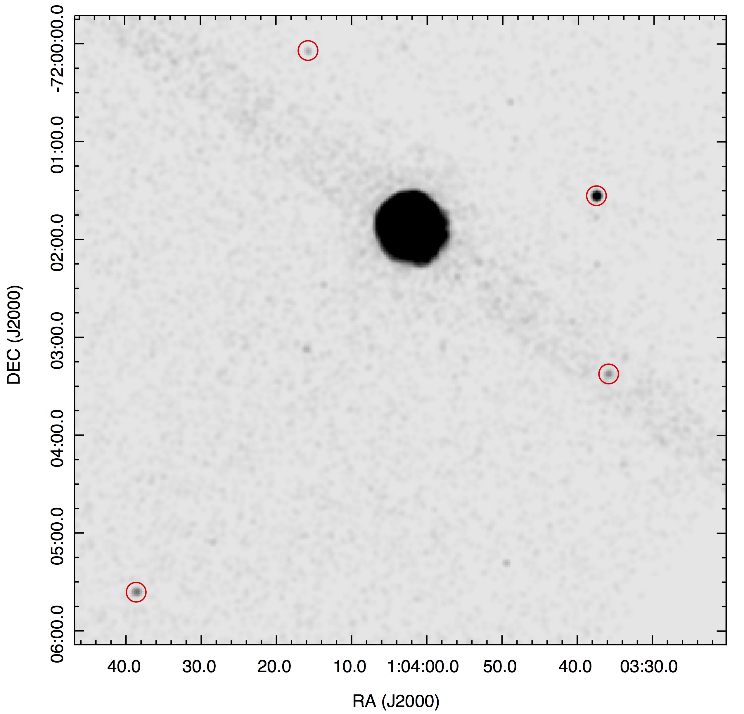
Figure 3: Point sources used for estimating systematic registration uncertainty.

Table 4: Comparison of shift results (in arcsec) using the Point Source (PS) and Central Knot registration methods

Observation	5123	5130	6074	6766
mean X PS shift	-0.11	-0.15	-0.14	-0.13
mean Y PS shift	-0.03	-0.14	-0.06	-0.24
registration X shift	-0.11	-0.14	-0.11	-0.19
registration Y shift	-0.01	-0.26	-0.01	-0.06
mean residual X	-0.03
mean residual Y	-0.09

3.4 Spectral Analysis

We conducted a spectral analysis to convince ourselves that the regions we are using to measure the expansion of the blastwave or forward shock exhibit spectral properties consistent with swept-up interstellar material in the SMC and to derive a temperature that can be used to infer a shock velocity.

We extracted spectra from five regions near the outer extent of the X-ray emission as shown in Figure 2 (top panel), which we believe to be representative of the forward shock emission. The regions have been adjusted to follow the curvature of the emission. The widths of the regions are $1.0\arcsec$ to sample as small a region behind the forward shock as possible while maintaining sufficient statistics for spectral analysis. We combined data from 36 Chandra observations to maximize the counts in the extracted spectrum (ObsIDs: 1308, 1311, 1530, 1531, 2843, 2844, 2850, 2851, 3520, 3544, 3545, 5123, 5124, 5130, 5131, 6042, 6043, 6074, 6075, 6758, 6759, 6765, 6766, 8365, 9694, 10654, 10655, 10656, 11957, 13093, 14258, 15467, 16589, 17380, 18418, 19850). We included fullframe and subarray data in these extractions since these regions are negligibly affected by pileup as shown in Figure 2 (bottom panels).

We fit the spectrum with a vpshock model in XSPEC (using the wilm abundances and the vern photoelectric constants) and allowed the abundances of O, Ne, Mg, and Fe to vary. We utilized a two-component model for the absorption, with one component for the Galactic line of sight absorption (tbabs), $N_{H},_{Galactic}=5.36\times 10^{20}cm^{-2}$ (Dickey & Lockman, 1990), and another with the SMC abundances specified in Russell & Dopita (1992) (tbvarabs) and the best fitted value of $N_{H},_{SMC}=5.76\times 10^{20}cm^{-2}$ determined from the XMM-Newton Reflection Gratings Spectrometer presented in Plucinsky et al. (2017). Both absorption components were held fixed.

A background model consisting of detector and sky background components was fit simultaneously with the source spectra. The data were unbinned for the fitting process (the data have only been binned for display purposes) and the C statistic was used as the fit statistic.

The fit with a single vpshock model produced an acceptable fit for all five regions with a C statistic of 440 to 480 for 489 degrees of freedom (DOF). The fitted parameters are shown in Table 5 and the spectral fits with residuals are shown in Figure 4. The temperatures for all 5 regions are consistent at the 1.0 sigma level. The $n_{e}t$ are consistent at the 1.25 sigma level. The spectral fit of only region s1 is shown in Figure 5, to demonstrate that the source dominates over the background for most of the energy range considered here even for regions as faint as these forward shock regions. The background region was selected to include emission on and off the transfer streak from E0102 itself. The amount of transfer streak emission that affects our spectral extraction regions varies from observation to observation (from negligile to at most 6%) as it depends on the roll angle of the observation on that date, which determines the orientation of the readout direction of the CCD on the sky. Our background spectrum, and hence model, partially accounts for this relatively low level of contamination from the transfer streak.

The results show that the blastwave region has typical ISM abundances for the SMC ($\sim 0.2-0.3$), although the Fe abundance is significantly lower than the expected SMC value. The Ne abundance is higher than the expected SMC value. This might indicate that the modeling has limited ability to distinguish Fe-L emission from Ne emission. These abundance values are much lower than the values in the bright ring which is dominated by ejecta emission from O, Ne, and Mg. Sasaki et al. (2001) derives abundances of $4.7^{+4.6}_{-0.3}$, $7.1^{+6.4}_{-1.2}$, & $3.0^{+0.3}_{-0.3}$ for O, Ne, & Mg respectively for the entire remnant assuming a two component vgnei model in XSPEC. We conclude that the regions from which we extracted a spectrum are consistent with interstellar material heated by the blastwave.

Table 5: Spectral Model Parameters for the Blast Wave Regions. The model is $\mathrm{TBabs\times TBvarabs\times vpshock}$. The $\mathrm{TBabs}$ component represents the galactic absorption, $N_{H},_{Galactic}=5.36\times 10^{20}cm^{-2}$, and the $\mathrm{TBvarabs}$ represents the SMC absorption of $N_{H},_{SMC}=5.76\times 10^{20}cm^{-2}$. The fitted elemental abundances of the $\mathrm{vpshock}$ component are listed in this table and the rest of the elemental abundances of the $\mathrm{vpshock}$ component are set to 0.2 solar abundances.

Parameters	S1	S2	S3	S4	S5
$kT_{e}\,\mathrm{(}keV)$	$0.65^{+0.14}_{-0.07}$	$0.75^{+0.06}_{-0.05}$	$0.70^{+0.09}_{-0.11}$	$0.71^{+0.10}_{-0.08}$	$0.61^{+0.06}_{-0.04}$
Oxygen	$0.23^{+0.05}_{-0.04}$	$0.27^{+0.05}_{-0.04}$	$0.29^{+0.10}_{-0.06}$	$0.27^{+0.04}_{-0.04}$	$0.24^{+0.05}_{-0.04}$
Neon	$0.37^{+0.07}_{-0.05}$	$0.29^{+0.04}_{-0.03}$	$0.36^{+0.07}_{-0.06}$	$0.36^{+0.06}_{-0.05}$	$0.31^{+0.04}_{-0.04}$
Magnesium	$0.30^{+0.10}_{-0.08}$	$0.13^{+0.04}_{-0.04}$	$0.20^{+0.09}_{-0.07}$	$0.30^{+0.09}_{-0.08}$	$0.21^{+0.06}_{-0.05}$
Iron	$0.06^{+0.04}_{-0.02}$	$0.06^{+0.02}_{-0.01}$	$0.04^{+0.02}_{-0.02}$	$0.10^{+0.03}_{-0.03}$	$0.04^{+0.01}_{-0.01}$
$n_{\mathit{e}}\,t,(10^{11}\,\mathrm{cm}^{-3}\mathrm{s})$	$1.50^{+0.99}_{-0.78}$	$1.53^{+0.51}_{-0.39}$	$2.32^{+2.83}_{-0.84}$	$1.10^{+0.59}_{-0.37}$	$2.24^{+0.93}_{-0.71}$
$Norm,(10^{-5})$	$2.02^{+0.51}_{-0.60}$	$4.76^{+0.57}_{-0.58}$	$2.16^{+0.77}_{-0.40}$	$5.57^{+0.57}_{-0.48}$	$4.50^{+0.66}_{-0.70}$
C-statistic (dof)	440(489)	477(489)	454(489)	480(489)	470(489)
Pearson $\chi^{2}$ (dof)	498(489)	503(489)	497(489)	487(489)	483(489)
goodness	0.63	0.67	0.63	0.55	0.35
counts($\mathrm{10^{3}}$)	1.67	2.77	1.54	2.21	2.82
area ($\mathrm{pixel^{2}}$)	61.32	69.63	76.50	80.19	80.63
Weighted by $\mathrm{counts}$
$kT_{e}\,\mathrm{(}keV)$			$0.68^{+0.05}_{-0.05}$
$n_{\mathit{e}}\,t,(10^{11}\,\mathrm{cm}^{-3}\mathrm{s})$			$1.73^{+0.46}_{-0.46}$

The fitted temperatures range from $0.61$ keV to $0.75$ keV, and the ionization time scales range from $1.10\times 10^{11}\;\mathrm{cm}^{-3}\;\mathrm{s}$ to $2.32\times 10^{11}\;\mathrm{cm}^{-3}\;\mathrm{s}$. All the fits are statistically acceptable. We computed a counts-weighted average temperature of ${\mathrm{kT}_{\mathit{e}}}=0.68^{+0.05}_{-0.05}\;\mathrm{keV}$ and counts-weighted average ionization timescale of ${n_{\mathit{e}}\,t}=1.73^{+0.46}_{-0.46}\times 10^{11}\,\mathrm{cm}^{-3}\,\mathrm{s}$. We will adopt these weighted values for the temperature and ionization timescale for calculations in §4.3.

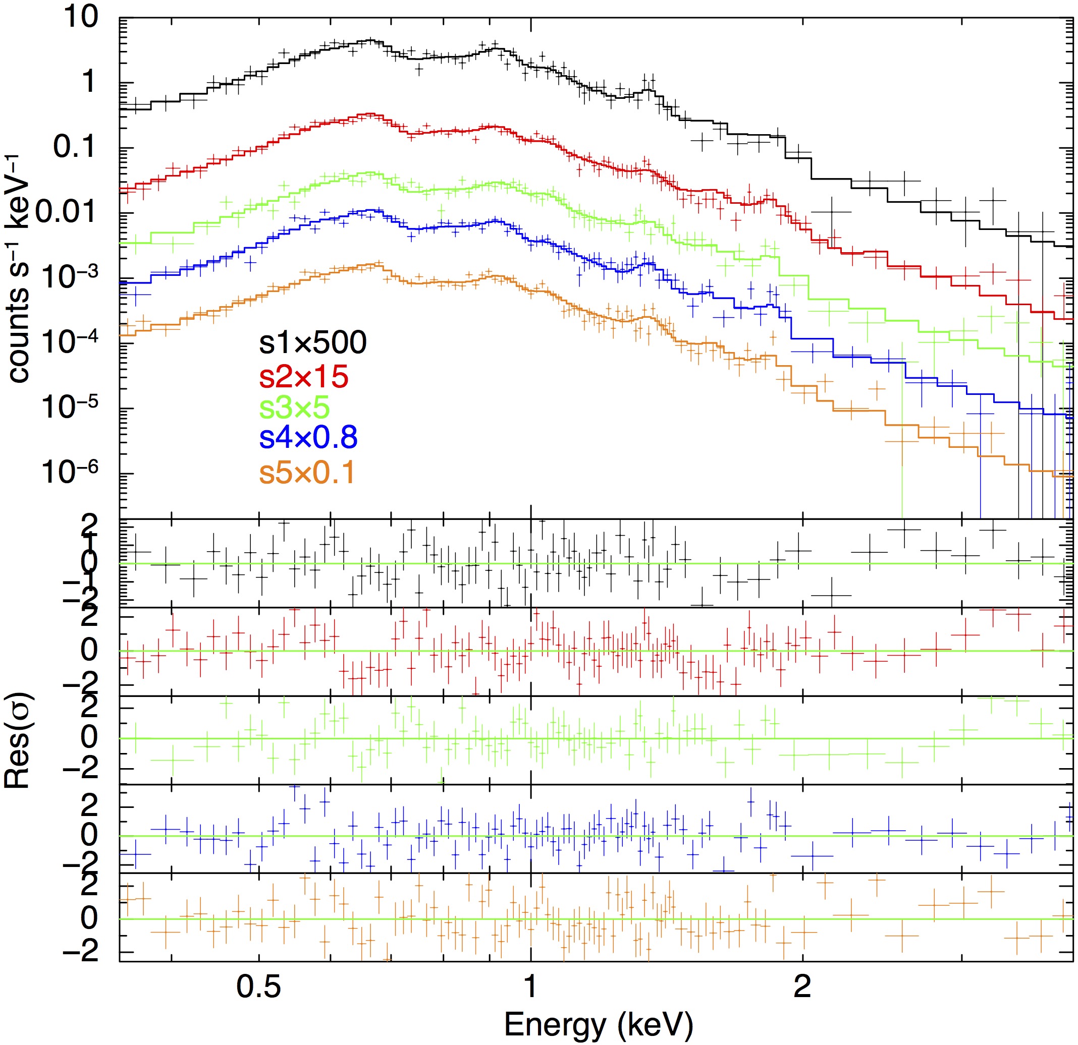
Figure 4: Spectrum of the blast wave regions shown in Figure 2 (top panel). The data are fit with a vpshock model with parameters listed in Table 5. The spectral data have been binned for display purposes only and an explicit background model and data (not shown) were fit simultaneously with the source model.

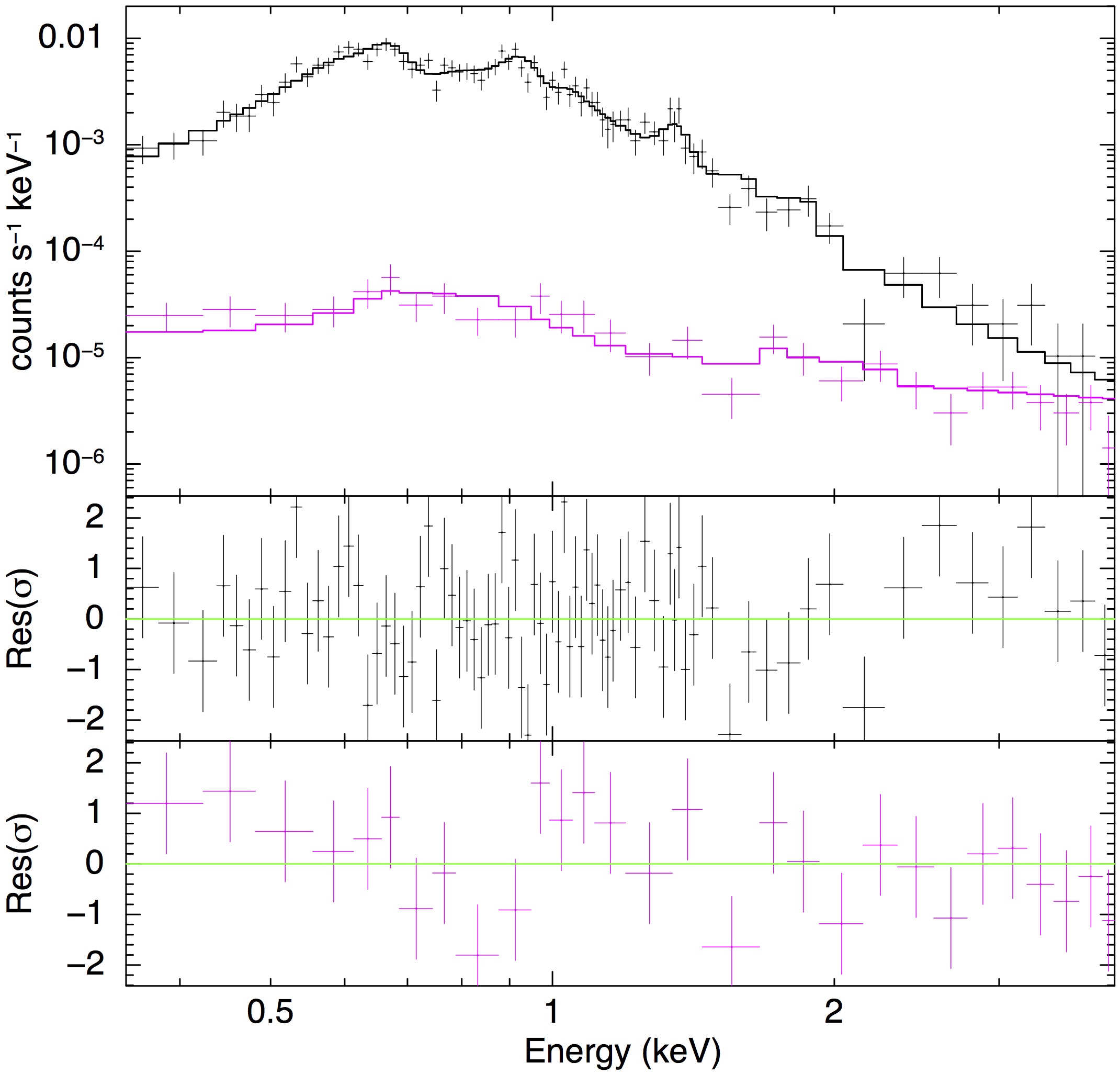
Figure 5: Spectrum of region s1 shown in Figure 2 (top panel). The data are fit with a vpshock model with parameters listed in Table 5. The spectral data have been binned for display purposes only and an explicit background model and data were fit simultaneously with the source model. The black data points and solid lines are for source data and model, respectively. The magenta data points and solid lines are for background data and model, respectively.

3.5 Radial Profile Analysis

We extract 1-dimensional radial profiles from the model image generated from ObsID 1423 and the comparison observations, and fit them with a projected jump function to get the radius of the blast wave for each azimuthal direction. We then calculate the expansion as the difference between the two radii. We fit the radial profiles with a theoretical model instead of shifting the radial profile of one epoch and comparing to the radial profile of the data from another epoch as was done by Katsuda et al. (2008) for G266.2-1.2 and Yamaguchi et al. (2016) for RCW 86 because the expected magnitude of the shift for E0102 is much smaller due to the fact that the distance to E0102 is 20-50 times larger than the distances to RCW 86 and G266.6-1.2. The expected expansion of the blast wave of E0102 is $0.35\arcsec$ for a 16 year baseline, which is comparable to the $0.246\arcsec$ bin size we have used for our radial profiles. For comparison, Katsuda et al. (2008) measure shifts as large as $6.0\arcsec$ for G266.2-1.2 and Yamaguchi et al. (2016) measure shifts as large as $2.7\arcsec$ for RCW 86 which are several times larger than their bin sizes. In addition, the E0102 data have significantly fewer counts per bin than the G266.2-1.2 and RCW 86 data which further motivates us to adopt the model-fitting approach. Williams et al. (2018) adopted the approach of measuring the expansion of N103B in the LMC along four diameters rotated with respect to each other to form two orthogonal coordinate systems. They computed the average of the expansion values on both sides of the diameter and adopted the average as their best estimate of the expansion since the values can be significantly different on either side and were in fact negative for one side of one diameter. Using this method, Williams et al. (2018) find an average expansion of $0.31\arcsec$ over a 17.4 yr baseline which corresponds to a shock velocity of $4170~{}\mathrm{km}\,\mathrm{s}^{-1}$.

The expansion for each direction is calculated from:

$$f_{exp}=\frac{R_{2}-R_{1}}{R_{1}},$$ (2)

where $R_{1}$ and $R_{2}$ are the radii of the remnant to the geometric center listed in Table 8, from the model and later observation, respectively. We adopt the estimate of the geometric center from Milisavljevic listed in Table 8, see § 3.7 for details.

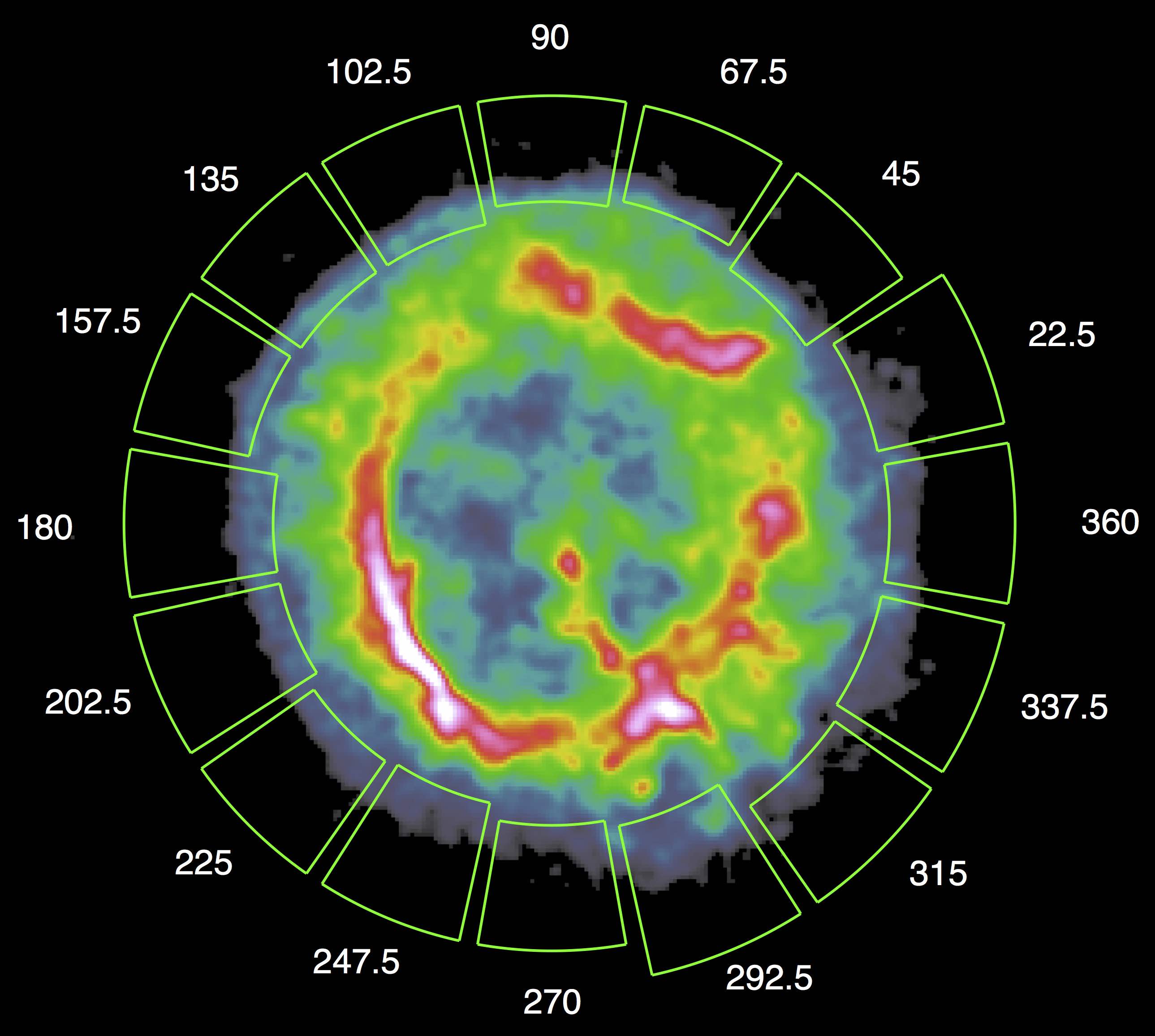
Figure 6: The image from ObsID 1423 with the radial profile extraction regions overplotted. The radial profile extraction regions are indicated in green and the angular position are indicated in white. The widths of the regions vary depending on the structure of the remnant at that angular position.

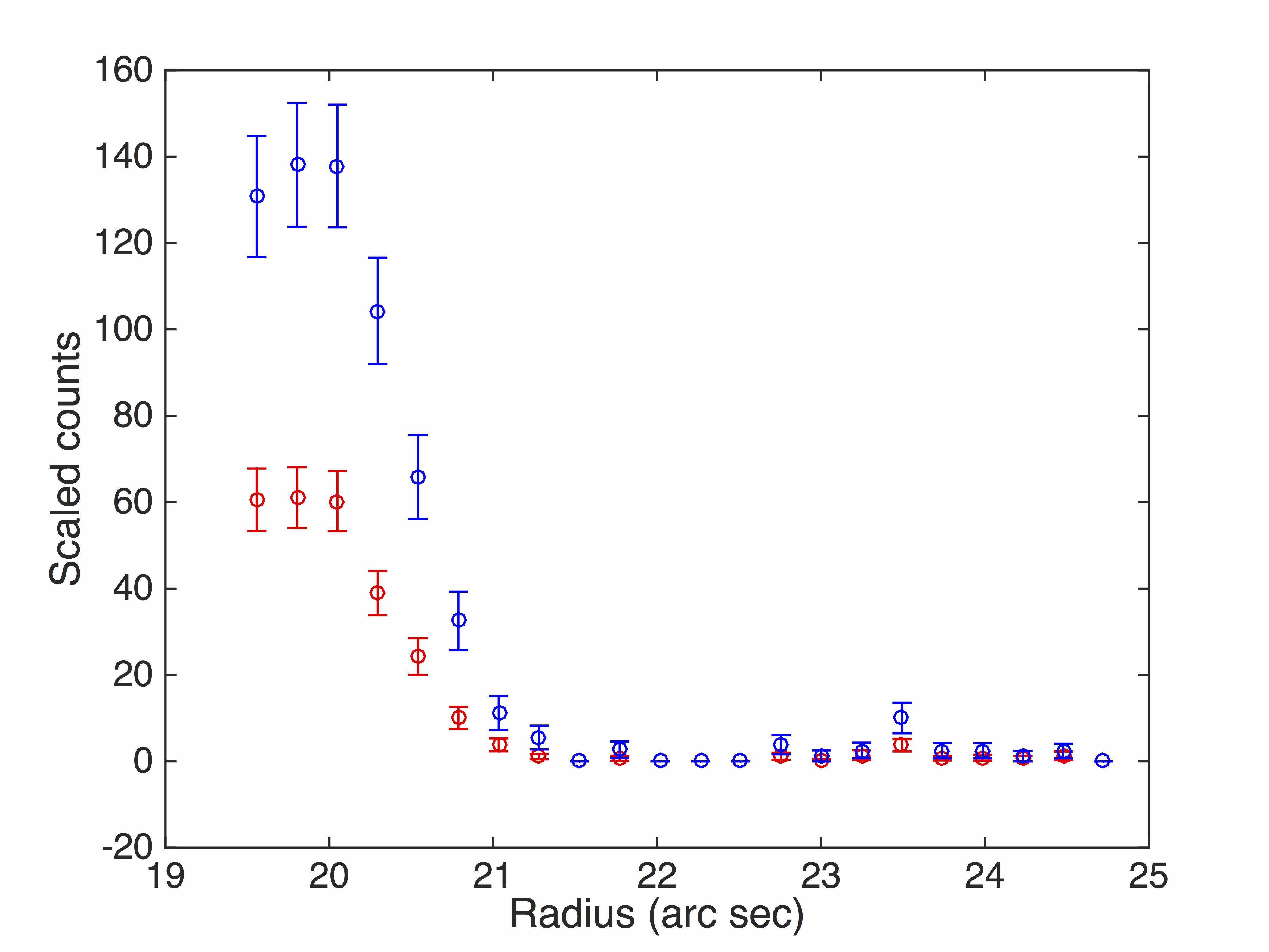
Figure 7: Radial profile from ObsID 1423 with and without correction for the QE decrease. The blue points are from ObsID 1423 itself. The red points show the radial profile after correction for the loss of QE appropriate for the date of ObsID 17380.

The radial profiles are extracted from 16 azimuthal sectors, each covering $20^{\circ}$, and the position angles of these sectors start from $0^{\circ}(\equiv 360^{\circ})$ west, increasing counter-clockwise, stepping by $22.5^{\circ}$ increments to $337.5^{\circ}$ as shown in Figure 6. For each sector, the number counts in a radial bin at radius $r$ is obtained by the CIAO tool dmstat summing the events within the region between radii of $r\pm 0.123\arcsec$. For the radial profiles from ObsID 1423, the counts in a bin are calculated by summing the events within the region and then weighting by the quantum efficiency loss and exposure time difference. Figure 7 shows the radial profile from ObsID 1423 for the azimuthal direction $\theta=135$. The blue curve shows the radial profile for ObsID 1423 itself while the red curve shows the radial profile after it has been corrected for the decrease in QE appropriate for the date of ObsID 17380. The area of an annular sector with a given radial width decreases as the annulus radius, $r$, decreases. The counts at $r$ are scaled with the ratio of the area of outermost region to the area of region at $r$. Note that the data for the radial profiles for the model image are not smoothed, smoothing was only applied to the model image used for registration. The C statistic was used for fits to the radial profiles as there are bins in the radial profile that have 0, 1, or 2 counts in the regions at larger radii than the forward shock; for plotting purposes, the Gehrels (1986) approximation ($\mathrm{error}=1+\sqrt{\mathrm{counts}+0.75}$) was used as the uncertainty on the data points.

3.6 Radial Profile Model

To fit the radial profiles, we construct a model function which assumes a thin spherical shell of emitting material (in projection). The model profile is constructed by taking a slice through the thin spherical shell. These profiles are convolved with a 1D Gaussian function with $\sigma=0.492\arcsec$ to account for the PSF of Chandra. Figure 8 displays the model after it has been convolved with the PSF. The emissivity function is assumed to be a step function with uniform intensity behind the blast wave, which is:

$$e(r)=\begin{cases}I&\quad\text{if }R\geqslant r\geqslant R-d\\ 0&\quad\text{if }r>R\\ \end{cases}$$

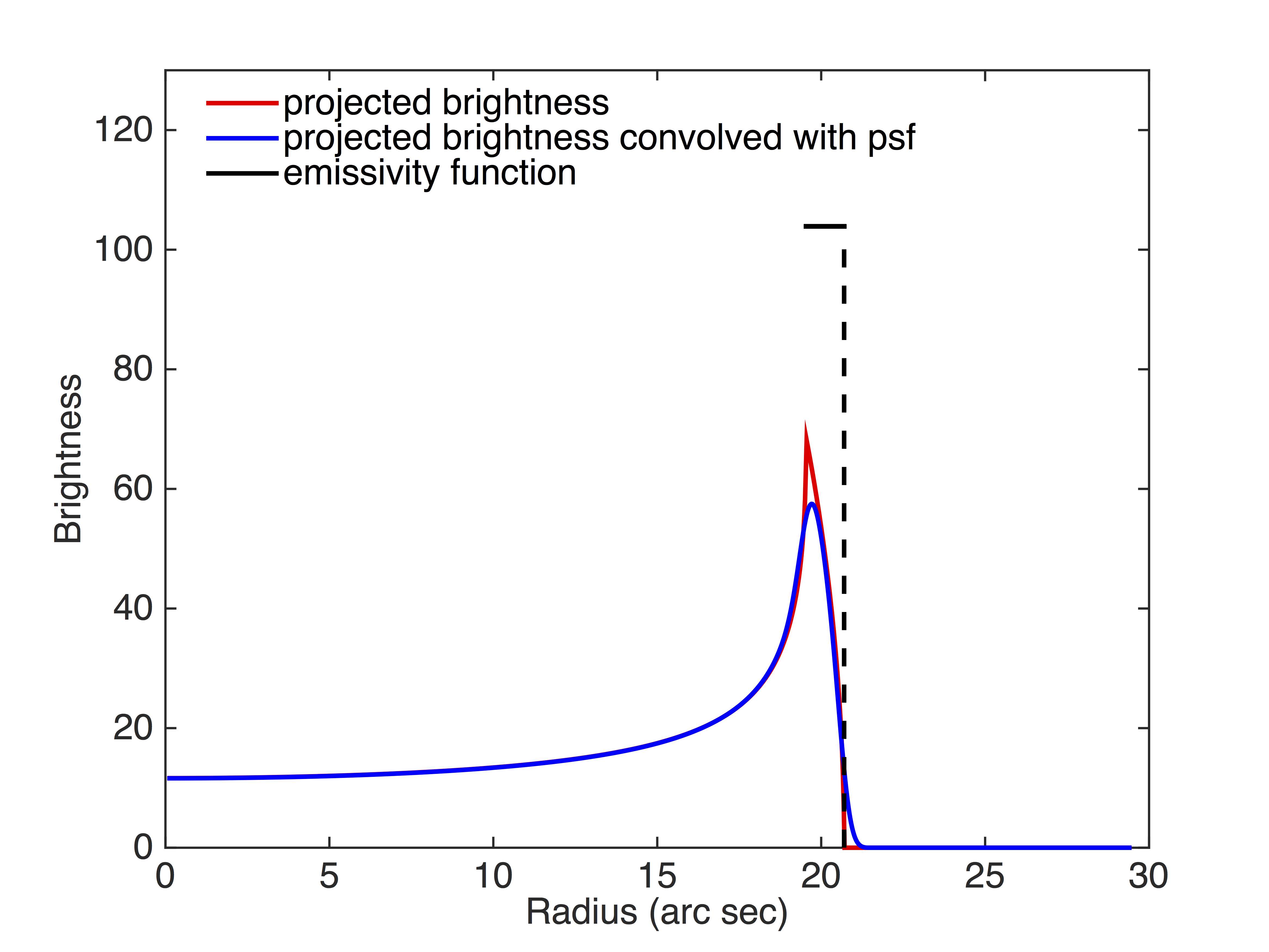
Figure 8: Model for fitting the radial profiles. The red curve gives the projection along the line-of-sight assuming the black emissivity function. The blue curve gives this distribution after it has been convolved with the Chandra PSF.

Here, $I$ is intensity, $R$ is the radius of the blast wave, and $d$ is the width of blast wave. For fitting the 1D radial profiles, there are 4 free parameters, 3 of them from the shell emission model, $I$, $R$ and $d$, and the 4th is an additive uniform background level, $b$. We fit the profiles from ObsID 1423 first. Then the model with fixed $I$ and $d$, obtained from fitting profiles of ObsID 1423, is used to fit profiles from later observations, as these two values are not expected to change significantly with a time difference of up to 16 years. The free parameters for the fits to the comparison data images are $R$ and $b$. In this manner, we fit for the radii of the blast wave from 1423, $R_{1}$, and from later observations, $R_{2}$ in each of 16 directions. Some sample fits are shown in Figure 9 for three different angular positions from ObsID 17380 compared to ObsID 1423. The shape of the distributions for the radial profiles from ObsID 17380 are the same as those for ObsID 1423, the only parameters that change for the ObsID 17380 fits are $R_{2}$ and $b$. The differences for the radii in the 16 directions are tabulated and used in the next step of the analysis.

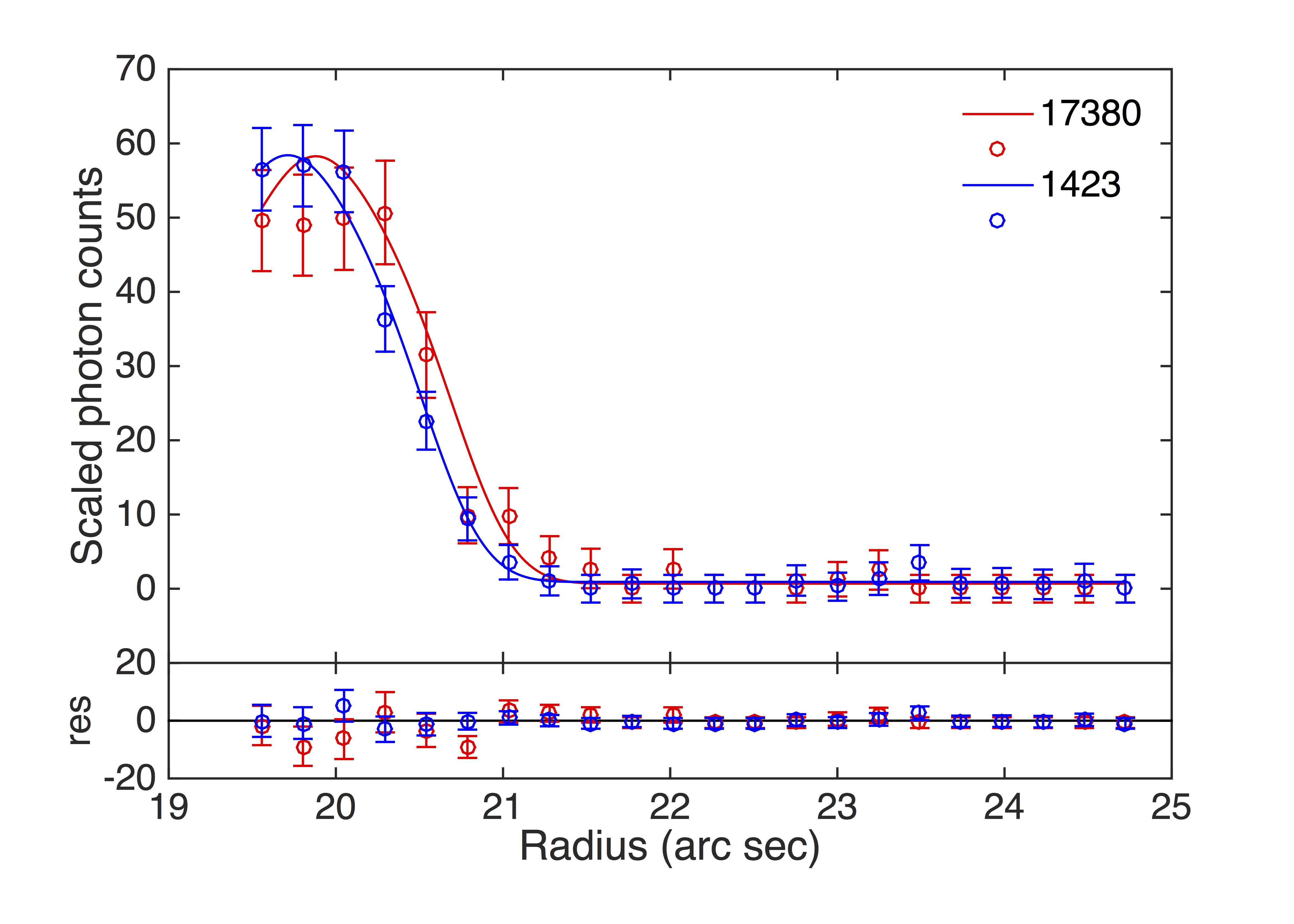
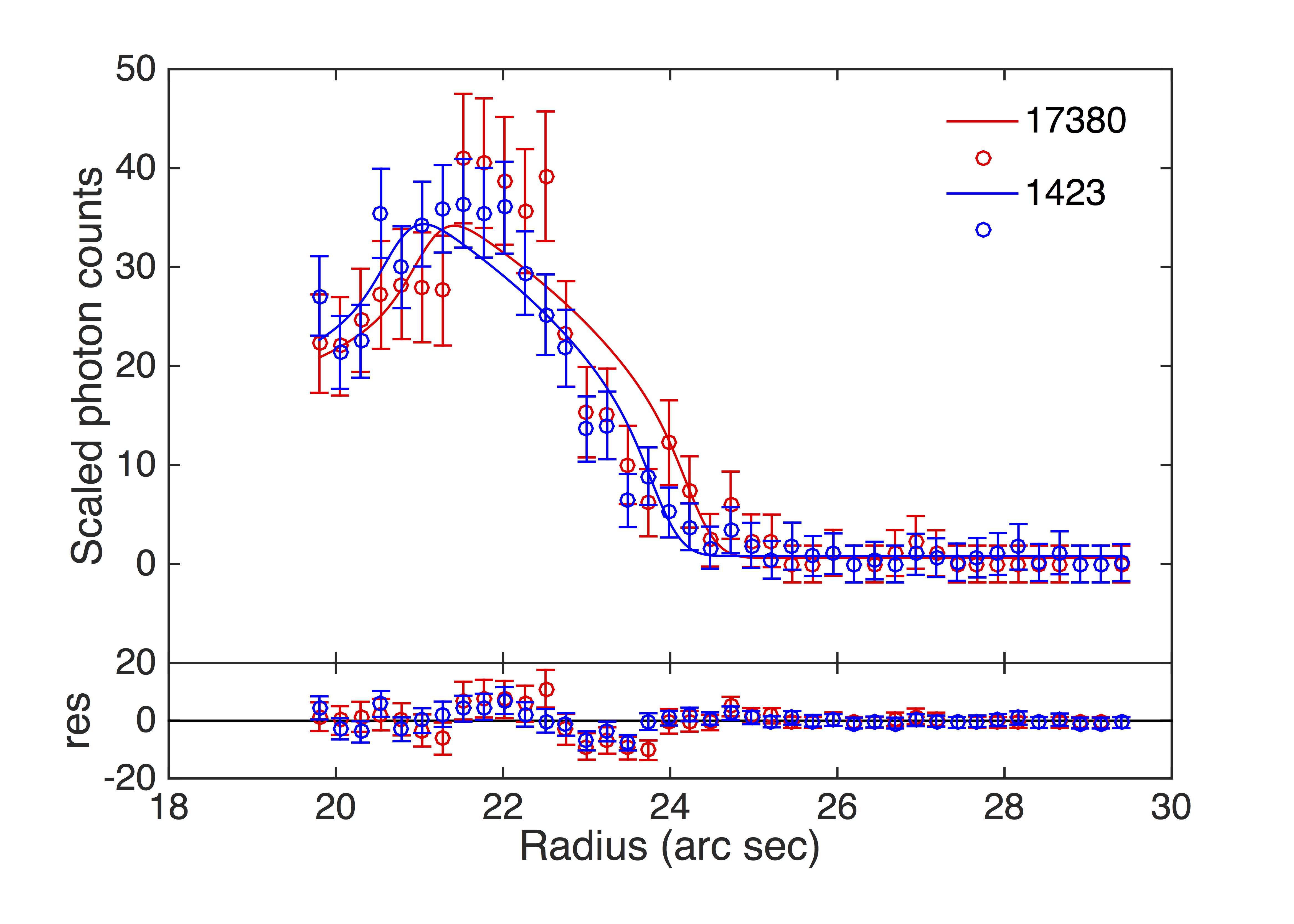
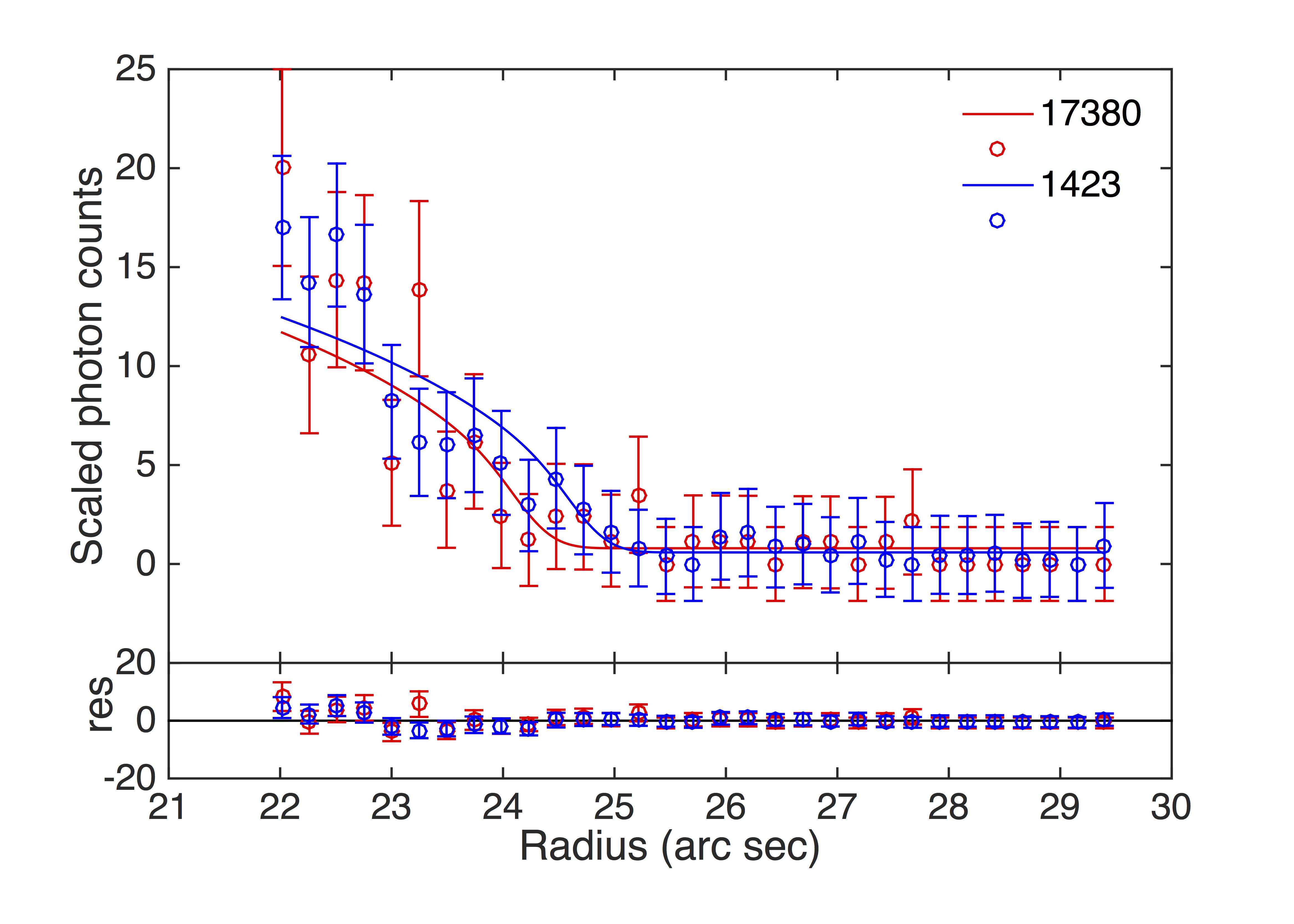
Figure 9: From top to bottom: radial profiles for azimuthal positions 135, 292.5, and 315 from ObsIDs 1423 and 17380.

3.6.1 Registration Bias Correction

Our expansion results are sensitive to any remaining bias or systematic uncertainty (see §3.3.2) in the registration of the model image to the comparison data images. We can estimate this bias by examining the radial differences computed in the previous section as a function position angle around the remnant. Any bias in the registration would tend to increase/decrease the measured expansion in one direction while decreasing/increasing the expansion in the direction $180\arcdeg$ opposite. Such a bias would manifest itself as a sinusoidal pattern in the radial differences as a function of position angle. An incorrect choice of the center for the annular sectors will also produce a sinusoidal variation, degenerate with the registration error. The uncertainties are large enough that it is impractical to extract azimuthal variation of the expansion, so we estimate an average expansion by zeroing out the sinusoidal component. To correct for this bias, we fit the radial profile differences as a function of position angle with a model that has as parameters a shift in X and Y and the average expansion rate. For each test data (ObsID $i$) and for the reference (model) data we have radial profile differences as a function of position angle, $\theta_{\mathit{j}}$, $j=1\cdots 16$. For test data ObsID $i$ and reference data ObsID $i_{0}$, the profile difference for position angle $\theta_{\mathit{j}}$ is

$$\delta R_{\mathit{j,i}}=r_{\mathit{i}}(\theta_{\mathit{j}})-r_{\mathit{i_{0}}}(\theta_{\mathit{j}})$$ (3)

The sinusoidal fit function has the form:

$$\delta R_{\mathit{j,i}}=\Delta X_{\mathit{i}}\cos\theta_{\mathit{j}}+\Delta Y_{\mathit{i}}\sin\theta_{\mathit{j}}-\Delta R_{\mathit{i}}$$ (4)

where the $\delta R_{\mathit{j,i}}$ are the measured profile differences, $\Delta X_{\mathit{i}}$ and $\Delta Y_{\mathit{i}}$ are the residual offset errors in the $X$ and $Y$ registration, and $\Delta R_{\mathit{i}}$ is the expansion estimate for observation $i$ relative to observation $i_{0}$. The confidence intervals for the parameters are determined by the square roots of the diagonal entries of the covariance matrix, $\mathrm{cov}(\hat{\beta})$, where $\hat{\beta}$ is the least-squares estimator for $\beta=(-\Delta X_{\mathit{i}},-\Delta Y_{\mathit{i}},\Delta R_{\mathit{i}})$.

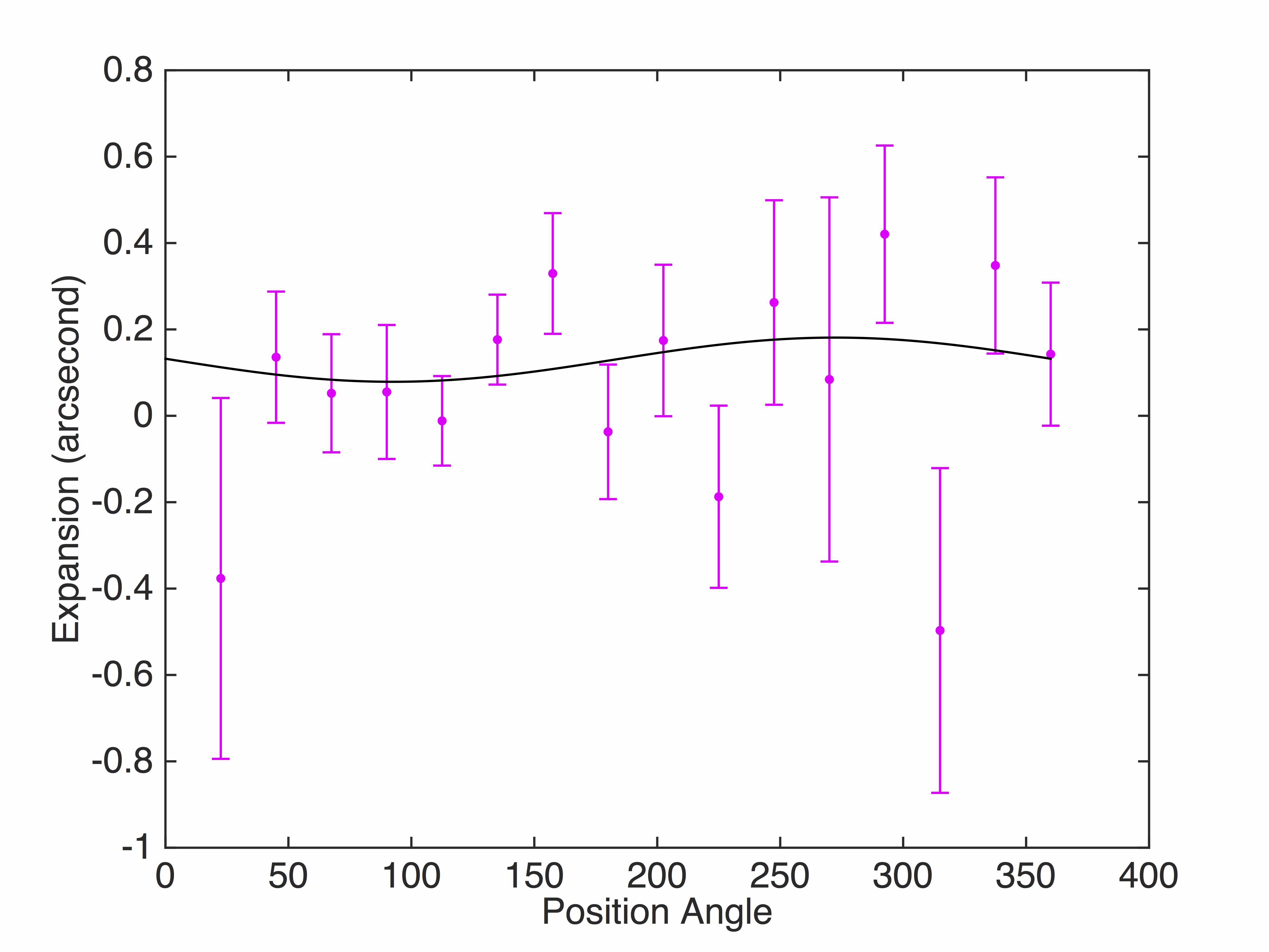
Figure 10: Expansion measurements as a function of azimuthal position for ObsID 17380. The black curve is the best fit for the model described in Equation 4.

With the expansion rates in 16 directions and an assumption of an approximately spherical geometry, we can obtain a global expansion rate for each pair of observations and the shift between the center of the two observations by fitting the expansion rates versus position angles with a sinusoidal function. By adopting this model, we are implicitly assuming that the expansion is the same in all 16 directions. This clearly is not the case in many SNRS – see, for example, Vink (2008) for the case of Kepler’s SNR. But it can be argued that the expansion of E0102 must be close to uniform around the remnant, based on the smooth, approximately symmetric outer extent of E0102. A sample fit for ObsID 17380 is shown in Figure 10. The uncertainties on the data are determined from the uncertainties on the fitted radii from the radial profile fits. It is clear that some directions have significantly larger uncertainties, such as $\theta=22.5,\;270.0,\;\mathrm{and}\;315.0$. As is seen in Figure 6, these directions do not have a smooth, outer contour and hence the uncertainty on our radial profile fit is larger as our assumed model does not represent the data as well as it does in other directions. The results of the fitted registration biases are listed in Table 6. The uncertainties for $\Delta X$, $\Delta Y$, $\Delta R$ are the 1.0 $\sigma$ statistical uncertainties from the sinusoidal fits. As expected, the fitted shift values are small (less than $0.1\arcsec$ in all but two cases) and the average of the shift values is close to zero indicating a symmetric distribution of positive and negative shifts. The average of the magnitude of the shift in the X direction is $0.05\arcsec$ and in the Y direction is $0.09\arcsec$. This is consistent with our estimate of the systematic uncertainty in §3.3.2.

Table 6: Registration Bias and Fitted Radial Shifts

ObsID	$\Delta\mathrm{X}$	$\sigma_{\Delta\mathrm{X}}$	$\Delta\mathrm{Y}$	$\sigma_{\Delta\mathrm{Y}}$	$\Delta\mathrm{R}$	$\sigma_{\Delta\mathrm{R}}$
	(arc sec)	(arc sec)	(arc sec)	(arc sec)	(arc sec)	(arc sec)
3545	0.03	0.07	0.00	0.07	0.08	0.05
6765	-0.07	0.06	-0.16	0.07	0.04	0.05
6766	-0.01	0.06	0.04	0.06	0.04	0.04
9694	-0.02	0.06	-0.03	0.06	0.07	0.04
11957	0.08	0.06	-0.17	0.06	0.02	0.04
13093	0.04	0.06	-0.12	0.06	0.05	0.04
14258	-0.04	0.06	-0.07	0.06	0.01	0.04
15467	-0.04	0.05	0.05	0.06	0.10	0.04
16589	-0.15	0.07	-0.08	0.08	0.08	0.06
17380	-0.00	0.06	0.05	0.06	0.13	0.05
18418	0.06	0.06	-0.21	0.07	0.09	0.05
mean shift x	-0.01	mean shift y	-0.06
mean |x|	0.05	mean |y|	0.09

Table 7: Expansion Result and Shock Velocity for E0102.

Expansion ($\%/{\rm yr}$)	Shock velocity (km/s)
$0.025\pm 0.006$	$1614\pm 367$

For each of the 11 comparison data images, the mean expansion rate and its uncertainty are listed in the last two columns of Table 6. We include the latest full-frame observation, ObsID 6766, from 2006 in these results. The evolution of the global expansion rate with time is shown in Figure 11. The data points are the measured expansions (percent) from the sinusoidal fits. The percent expansion versus time data were fit with a linear function, constrained to go through 0 at ${\rm t=0}$, to determine the best fitted value of the expansion rate. It is worth noting that the magenta data point from ObsID 6766 is consistent with the adjacent data points and the best fitted line. This indicates that our registration method using the central bright knot produces consistent results when compared to registration with point sources. Our measured expansion and the resulting shock velocity are listed in Table 7. We derive a rate of $0.025\pm 0.006\%~{}\rm{yr}^{-1}$ which is lower than the HRD00 result of $0.100\pm 0.025\%~{}\rm{yr}^{-1}$. As described in the introduction, we are measuring the expansion of the forward shock while HRD00 measured the global expansion of the remnant.

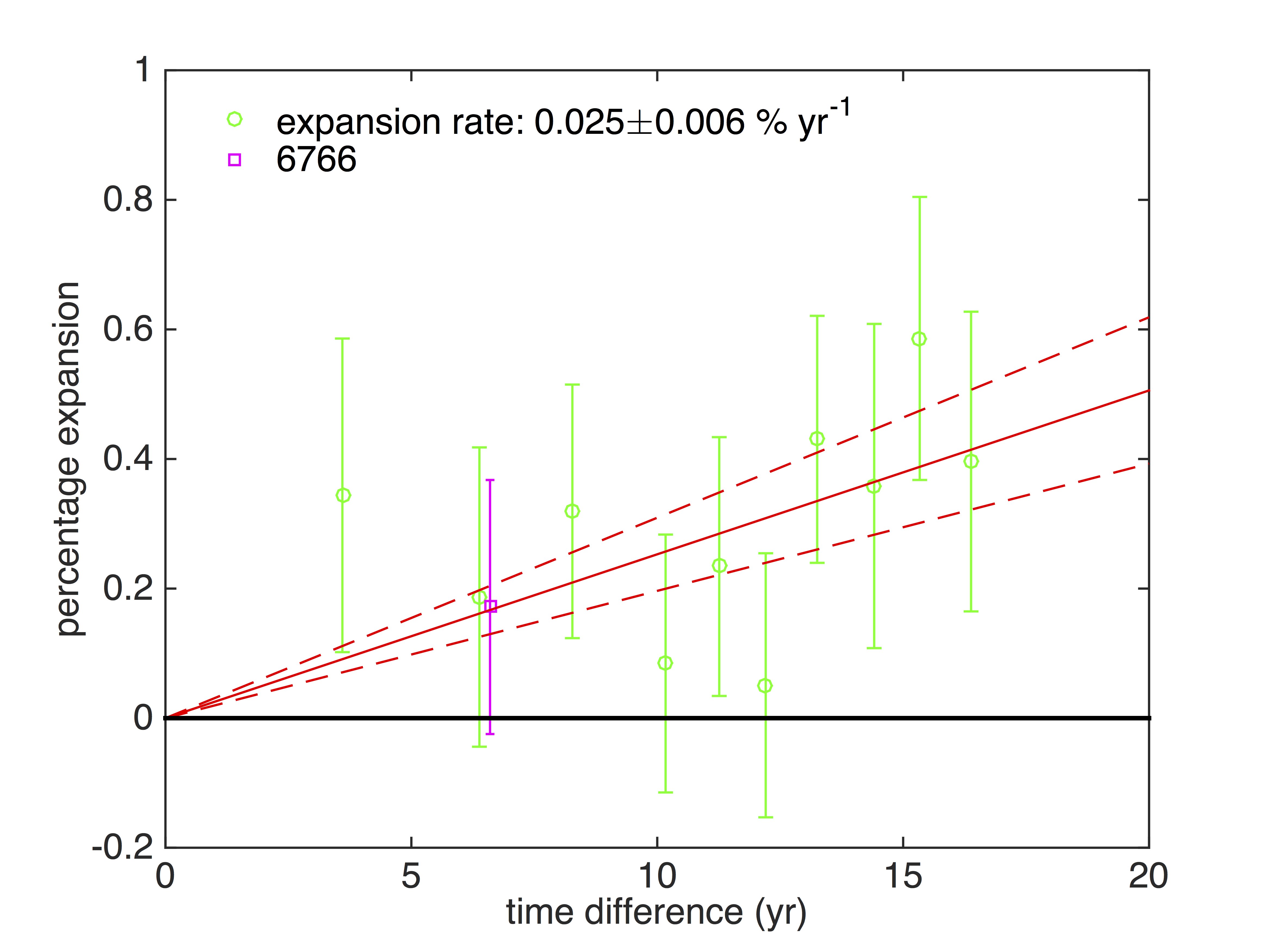
Figure 11: The expansion measured in $\%$ versus time. The green data points are the expansion rates measured by our method with the $1\sigma$ statistical uncertainties. The magenta point is for ObsID 6766, the one observation for which we could register the images using point sources. The red line is the best fit line that is constrained to go through zero at ${\rm t=0}$ and the dashed red lines are the $1\sigma$ uncertainties on the slope.

3.7 Determination of the Forward and Reverse Shock Radii

Table 8: Estimates of the Geometric Center

Geometric centers	RA	DEC
Finkelstein et al. (2006)	01h 04m 2.08s	$-72^{\circ}\,01\arcmin\,52.5\arcsec$
Milisavljevic†	01h 04m 2.354s	$-72^{\circ}\,01\arcmin\,53.23\arcsec$
Ellipse of reverse shock	01h 04m 2.048s	$-72^{\circ}\,01\arcmin\,52.75\arcsec$
Ellipse of forward shock	01h 04m 1.964s	$-72^{\circ}\,01\arcmin\,53.47\arcsec$

^†private communication

We estimate the position of the forward and reverse shocks using radial profiles extracted in the 16 directions described previously. For the forward shock position we adopted the value determined from our fits to the radial profile with the model that assumed a thin spherical shell geometry and blurring from the Chandra PSF. For the reverse shock we determined the point at which the emission increased to its peak value moving outward from our adopted center of the remnant. In this manner, we derived 16 points each for the forward and reverse shock around the remnant. If E0102 were perfectly spherically symmetric, we could fit the 16 points with a circle for both the forward and reverse shock to determine the radius and center. However, the morphology does deviate from spherical symmetry as indicated by the larger extent of the forward shock in the southwest. The morphology of the reverse shock is more complicated as indicated by the apparent elliptical shape and the bright feature in the northwest that is apparently concave compared to the generally convex shape of the rest of the ring. The apparent elliptical morphology of the bright ring is consistent with the idea presented in Flanagan et al. (2004) that the ejecta consist of two rings, one red-shifted and one blue-shifted, or a cylinder which is expanding. In this idea, our line-of-sight is looking nearly down the major axis of the rings/cylinder. Given this morphology, we fit the 16 points for the forward shock with an ellipse with the center, position angle, and semi-major and semi-minor axes free. We applied the same approach for the 16 points for the reverse shock. We compare the values of the ellipse centers from the fits to the forward and reverse shocks to the values of F06 and Milisavljevic 2017 (private communication) in Table 8 and in Figure 12. There is excellent agreement between the centers derived from our fits and the centers derived from the optical expansion results. The fitted values for the semi-major, semi-minor axes, and rotation angle are displayed in Table 9. We determine the radius of the forward shock to be $6.34\pm 0.10$ pc and the radius of the reverse shock to be $4.17\pm 0.12$ pc. For the forward shock we take the average of the semi-major and semi-minor axis radii (see Table 9) with the range of values providing an estimate of the systematic uncertainty. For the reverse shock, we adopt the semi-major axis for the radius, appealing again to the concept of overlapping rings and/or a cylindrical geometry seen somewhat off-axis, and adopt the statistical uncertainty on the fit as the uncertainty. If we assume the X-ray bright ring is circular in nature and appears elliptical due to our off-axis viewing angle, we can estimate that angle from our measured ellipticity. From the minor and major axis values in Table 9, we estimate an angle of ${31^{\circ}}^{+6^{\circ}}_{-7^{\circ}}$.

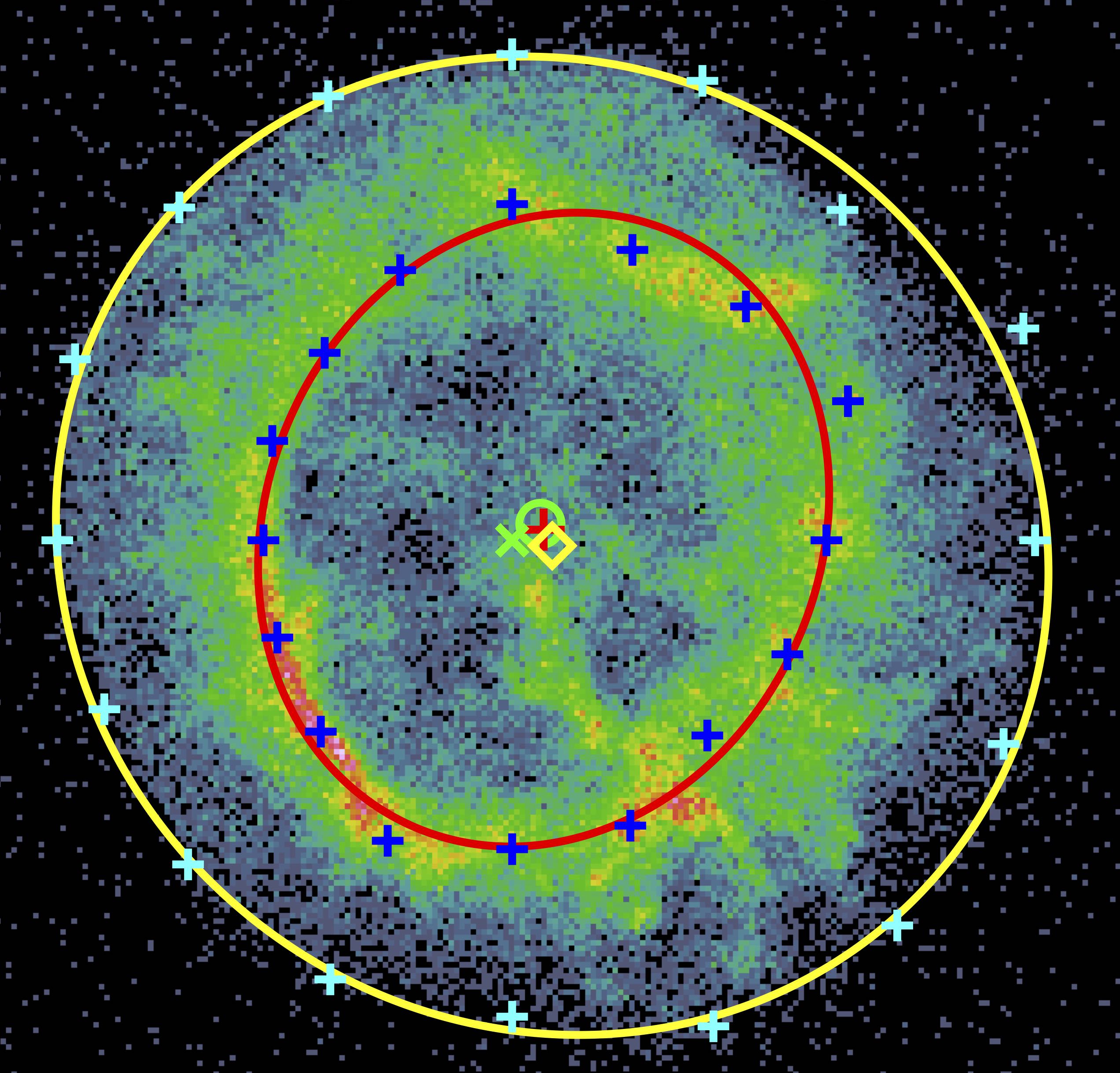
Figure 12: The ellipse fits for the forward and reverse shocks. The center positions are: Milisavljevic center (green $\times$), F06 center (green circle), fit based on X-ray radial profiles for the reverse shock (red crosses) and for the forward shock (yellow diamond).

Table 9: Fitted Values for the Ellipses for the Forward and Reverse Shocks

Parameters	Unit	Forward shock	Reverse shock
xc error	arcsec	0.074	0.023
yc error	arcsec	0.075	0.072
Major Axis	pc	$6.52^{+0.12}_{-0.12}$	$4.17^{+0.12}_{-0.12}$
Minor Axis	pc	$6.16^{+0.16}_{-0.12}$	$3.57^{+0.12}_{-0.13}$
Rotation Angle	degree	$-37.61^{+2.67}_{-2.69}$	$65.85^{+1.16}_{-1.16}$
Radius	pc	$6.34^{+0.10}_{-0.10}$	$4.17^{+0.12}_{-0.12}$

4 One Dimensional Shock Models

We generate analytic solutions following the work of Truelove & McKee (1999, 2000), as extended by Laming & Hwang (2003), Hwang & Laming (2012) and Micelotta et al. (2016). Truelove & McKee noted that the Euler equations do not contain any dimensioned parameters, and that dimensional aspects are introduced through the initial conditions. They introduced “unified solutions”, single dimensionless solutions merging similarity solutions for the initial ejecta dominated stage (Chevalier, 1982) through to the asymptotic Sedov-Taylor similarity solution (Sedov, 1959; Taylor, 1950). Three dimensioned parameters are introduced, $E$, the energy of the ejecta (explosion energy), $M_{\mathit{ej}}$, the mass of the ejecta, and $\rho_{0}$, the mass density of the preshock medium

The models assume an initial ejecta distribution expanding homologously with $v\propto r$ up to a maximum velocity $v_{\mathit{ej}}$ at the edge of the ejecta. The ejecta profile is given as

$$\rho_{\mathit{ej}}(r,t)=\rho_{\mathit{ej}}\left(v,t\right)\equiv\frac{M_{ej}}{\left(v_{\mathit{ej}}\,t\right)^{3}}f\left(\frac{v}{v_{\mathit{ej}}}\right)$$ (5)

where the dimensionless structure function, $f$ is

$$f(\omega)=\begin{cases}f_{0}&0\leq\omega\leq\omega_{\mathit{core}}\\ f_{n}\omega^{-n}&\omega_{\mathit{core}}\leq\omega\leq 1\end{cases}$$ (6)

with $\omega$ defined as

$$\omega\equiv\frac{v}{v_{\mathit{ej}}}$$ (7)

For steep power laws (large $n$) a constant density “core” is introduced. The core is taken to have constant density for simplicity; all that is required is that the core have a sufficiently shallow power law distribution. Truelove & McKee note that the distribution of mass and energy depends on $n$; for $n<3$, mass and energy are concentrated in the outer (high speed) ejecta, while for $n>5$, mass and energy are concentrated in the inner (low speed) ejecta. Based on Matzner & McKee (1999), it is expected that $n$ is relatively large, $n\gtrsim 7$. Our explorations showed that the results were relatively insensitive to $n$ for $n>7$; in our treatment below we set $n=9$.

The preshock ambient medium is also assumed to follow a power law distribution

$$\rho\propto\rho_{0}r^{-s}$$ (8)

where $s$ is 0 or 2, and $\rho_{0}$ is the ambient medium mass density just ahead of the shock. For the $s=0$ case (constant density ambient medium) the value of $\rho_{0}$ is constant. For the $s=2$ case (ambient density falls as $1/r^{2}$, appropriate for a constant stellar wind), the value of $\rho_{0}$ pertains to a particular choice for the blast wave radius, $R_{\mathrm{b,0}}$, so that $\rho(r)=\rho_{0}/(r/R_{\mathrm{b,0}})^{2}$. The introduction of a power law ambient medium density distribution does not introduce additional dimensioned constants and the ejecta structure function is a dimensionless function, so asymptotic similarity solutions can still be constructed. Note that the $r^{-2}$ ambient medium is assumed to be stationary ($v_{\mathit{wind}}\equiv 0$). This implies that the velocity of the constant wind should be much smaller than the forward shock velocity. Incorporating a significant wind velocity would introduce an additional dimensioned parameter, significantly complicating the solution.

Truelove & McKee (1999) produced a detailed treatment of the $s=0$ case, but only a limited treatment of the $s=2$ case. Hwang & Laming (2003), Laming & Hwang (2003), and Micelotta et al. (2016) extend the treatment to a more detailed consideration of the $s=2$ case. We refer the reader to these papers for the details. Here, we touch mainly on those aspects relevant to our analysis. In particular, we consider “swept-up” mass, and “unshocked ejecta”, subject to the caveat that the models are highly idealized, and that the actual situation is far more complex.

For swept up mass in the $s=2$ case, this is presumably the stellar wind of the progenitor, so swept-up mass plus ejecta mass plus $\sim 1.5\,M_{\sun}$ for a compact remnant would be a lower limit to the progenitor mass, since the blast wave radius may not have reached the edge of the stellar wind. We note that HST imaging (WFPC2 and ACS; Finkelstein et al., 2006) and Gaetz et al. (2000) show a partial “bowl” of [O III] emission, mostly complete southeast through west; if the [O III] emission is from the photoionized wind of the progenitor, the stellar wind likely extends no more than $\sim 1.5-2$ times the current blast wave radius. Note that for a $r^{-2}$ wind, the swept-up mass is proportional to the blast wave radius, so the above implies a factor of $\sim 2$ uncertainty in swept-up mass. In the case of $s=0$, such a simplistic interpretation is not available. The “constant density” preshock medium could be an average over some combination of progenitor mass loss and ambient medium.

Strong caveats are also necessary for the treatment of unshocked ejecta. We use this estimate as a sanity check, and for obtaining a rough idea of how much (unshocked) Fe might have been produced, since there is no definitive detection of substantial amounts of X-ray emitting Fe in E0102. The “unshocked” ejecta would also include ejecta emitting optically in [O III] and [O II] (Tuohy & Dopita, 1983) which have not yet been shocked to X-ray emitting temperatures.

4.1 Remnant Evolution

To describe the evolution of the blast wave and of the reverse shock $R_{\mathit{b,0}}$, so that $\rho(r)=\rho_{0}(r/R_{\mathit{b,0}})^{-s}$ for the $s=2$ case we follow Micelotta et al. (2016), while for the $s=0$ case, we follow Truelove & McKee (1999). The $s=2$ (constant wind) case is an oversimplification of the evolution of the star before the explosion; however, it is useful to contrast this with the uniform medium case.

Our models depend on three dimensioned parameters, $E_{51}$ (the explosion energy in units of $10^{51}\,\mathrm{erg}$), $M_{\mathit{ej}}$ (the ejecta mass in units of $\mathrm{M}_{\sun}$), and $\rho_{0}$ (the preshock ambient medium mass density), plus two dimensionless parameters ($n$, $s$), for a total of five adjustable parameters. The ambient medium mass density is related to the H number density $n_{0}$ by $n_{0}=(\rho_{0}/\mu_{\mathrm{H}})/(1\,\mathrm{cm}^{-3})$ where $\mu_{\mathrm{H}}$ is the mean mass per hydrogen nucleus, assuming cosmic abundances. As noted in §4, the solutions were relatively insensitive to $n$ for $n\geq 7$, and we adopt $n=9$. We consider the $s=0$ and $s=2$ cases separately. For each $s$ value, we consider ejecta masses of 2, 3, 4, 5, and 6 $\mathrm{M}_{\sun}$. Our observational constraints are the measured blast wave velocity, $v_{\mathit{b}}$, the observed blast wave radius, $R_{\mathit{b}}$, and the reverse shock radius, $R_{\mathit{r}}$ (based on the distance to E0102, taken to be 60.6 kpc, Hilditch et al., 2005). In each case, the other two free parameters, $E_{51}$ and $\rho_{0}$, are varied until until the blast wave velocity $v_{\mathit{b}}$, blast wave radius $R_{\mathit{b}}$, and reverse shock radius $R_{\mathit{r}}$ are matched.

Once the match is found, some derived quantities can be evaluated based on the parameters of the model: ejecta “core” mass, remnant age, reverse shock velocity $v_{\mathit{r}}$, swept-up mass, and unshocked ejecta mass. We estimate the swept-up mass by integrating the initial ambient medium profile out to the current blast wave radius, $R_{\mathit{b}}$. The unshocked ejecta mass is obtained from Eqs. 5 & 6 by integrating from $v_{\mathit{ej}}$ down to the reverse shock velocity $v_{\mathit{r}}$ making use of Eq. 7.

A deceleration parameter, $m$, for the blast wave, is also of interest. The blast wave radius $R_{\mathit{b}}$ varies with time as

$$R_{\mathit{b}}\propto t^{\mathit{m}}$$ (9)

where $m$ varies from $m=1$ (initial free expansion of the ejecta), to $m=2/5$ asymptotically as the Sedov-Taylor similarity solution is reached. The resulting values are given in Table 10.

Table 10: Models for ejecta profile $n=9$, $R_{b}=6.34$ pc, $R_{r}=4.17$ pc and $v_{b}=1614\mathrm{km~{}s}^{-1}$

Parameters	Symbol(units)			$s=2$					$s=0$
Ejecta mass	$M_{\mathit{ej}}(\mbox{$\mathrm{M}_{\sun}$})$	2	3	4	5	6	2	3	4	5	6
Explosion energy	$E(10^{51}\,\mathrm{erg})$	0.34	0.51	0.68	0.85	1.02	0.87	1.31	1.74	2.18	2.61
Circumstellar density	$\rho_{0}(\mathrm{amu~{}cm}^{-3})$	0.22	0.33	0.44	0.55	0.66	0.85	1.27	1.69	2.11	2.54
Swept-up mass	$\mathrm{M}_{\sun}$	17.4	26.1	34.8	43.5	52.2	22.1	33.2	44.2	55.3	66.3
core mass	$\mathrm{M}_{\sun}$	1.3	2.0	2.7	3.3	4.0	1.3	2.0	2.7	3.3	4.0
Unshocked mass	$\mathrm{M}_{\sun}$	0.06	0.09	0.12	0.15	0.18	0.05	0.08	0.10	0.13	0.16

Table 11: The age, reverse shock velocity, upstream ejecta velocity, downstream ejecta velocity, and expansion parameter for the s=2 and s=0 cases.

$\mathrm{Parameters}$	$\mathrm{Symbol(units)}$	$s=2$	$s=0$
Age	$\mathrm{yr}$	$2642^{+1002}_{-489}$	$1730^{+552}_{-400}$
Reverse shock velocity	$\mathrm{v_{r}(kms^{-1})}$	$923^{+413}_{-314}$	$37^{+306}_{-185}$
Upstream ejecta velocity	$\mathrm{v_{r,u}(kms^{-1})}$	$1544^{+369}_{-402}$	$2359^{+621}_{-597}$
Downstream ejecta velocity	$\mathrm{v_{r,d}(kms^{-1})}$	$1078^{+387}_{-333}$	$618^{+384}_{-288}$
Expansion parameter	$\mathrm{m}$	$0.69^{+0.06}_{-0.01}$	$0.45^{+0.01}_{-0.01}$

4.2 Model Results

The range of values in Table 10 may now be compared to theoretical predictions, measurements of other SNRs, and measurements at other wavelengths. The explosion energy of a single star is expected to range between $0.5-1.8\times 10^{51}$ ergs depending on the mass, metallicity and rotation of the progenitor (see Sukhbold et al., 2016, and references therein). The ejecta masses of the X-ray emitting O and Ne (the dominant constituents in E0102) have been estimated to be $\sim 5.7$ and $\sim 2.2\,\mbox{$\mathrm{M}_{\sun}$}$ respectively by Flanagan et al. (2004). However, they note that their assumption of a pure metal plasma results in the largest estimate of the ejecta mass and any hydrogen in the plasma would only reduce their ejecta estimates. This can be compared to estimates of $2-4\,\mbox{$\mathrm{M}_{\sun}$}$ for Cas A (Hwang & Laming, 2012). In addition to the ejecta observed in X-rays, there is also a contribution from the ejecta observed in the optical. A star with an initial mass of $25-40\,\mbox{$\mathrm{M}_{\sun}$}$ is considered to be capable of producing these large ejecta masses of O and Ne (see Nomoto et al., 1997; Sukhbold et al., 2016, and references therein). The masses of the most massive stars observed in the SMC have a maximum value of $\sim 90\,\mbox{$\mathrm{M}_{\sun}$}$ (Massey et al., 2000).

We are able to estimate the density of the preshock medium from our spectral fits described in §3.4. Adopting the normalizations in Table 5 to calculate the emission measure and assuming emission from a thin shell geometry, we derive an H number density of $n_{0}=0.86\pm\mathrm{0.03~{}cm}^{-3}$. There is at least a factor of two uncertainty on this calculation in addition to the statistical uncertainty due to our assumptions of the geometry and filling factor.

The estimated age and reverse shock velocity for the s=0 and s=2 cases are listed in Table 11. The results for the $s=2$ case indicate an age of $\sim 2600\;\mathrm{yr}$, a reverse shock velocity of $\sim 900~{}\mathrm{km}\,\mathrm{s}^{-1}$, and an expansion parameter of $\sim 0.7$. The age is larger than those estimated by F06 ($2122\pm 644$ yr and $2054\pm 584$ yr) but within the uncertainties. The reverse shock velocity and the expansion parameter indicate that the remnant has not yet reached the Sedov phase of evolution. The results for the $s=0$ case indicate an age of $\sim 1700$ yr, a reverse shock velocity close to zero, and expansion parameter that is quite close to the Sedov phase. The age estimate is consistent within the uncertainties to the F06 values and the relatively low values of the reverse shock velocity and expansion parameter are the result of the relatively high ambient densities required by the $s=0$ case to match the data.

Note that velocities estimated from the optical proper motions are expected to lie between the ejecta velocity upstream of the reverse shock, $v_{\mathrm{r,u}}$, (less the cloud shock velocity of $\sim 100\,\;\mathrm{km\,s^{-1}}$) and the fluid velocity, $v_{\mathrm{r,d}}$, downstream of the reverse shock. The $v_{\mathrm{r,d}}$ applies to a diffuse component undergoing a Rankine-Hugoniot jump at the reverse shock: we interpret this component as producing the X-ray emission. Optical emission requires much slower shocks ($\sim 100\;\mathrm{km\,s^{-1}}$ for [O III] emitting shocks). A natural explanation is that the [O III] emission results from “cloud” shocks driven into much denser material.

The properties of “shock/cloud” interactions were considered by McKee & Cowie (1975), and the issue has been extensively studied since. In essence, for a large overdensity $\chi=\rho_{\mathrm{cloud}}/\rho_{\mathrm{ambient}}$, the shock drives a slower shock into the cloud, and wraps around the cloud. The cloud expands laterally (increasing drag); the shock is subject to Rayleigh-Taylor and Richtmyer-Meshkov instabilities, and the sides are subject to Kelvin-Helmholtz instabilities. Eventually, the cloud is shredded and merges with the general postshock flow. The high density material initially moves ballistically, then slows, is shredded, and merges with the post reverse-shock flow. This implies that the velocities based on optical proper motions should lie between the initial free expansion (ballistic) velocity ($v_{\mathrm{r,u}}$) and the eventual post-reverse-shock flow ($v_{\mathrm{r,d}}$). Such a scenario was presented by Patnaude & Fesen (2014) to explain the correlation and lack of correlation between the optical and X-ray emission in Cas A. Our estimates of the $v_{\mathrm{r,u}}$ and $v_{\mathrm{r,d}}$ are included in Table 11. These values are consistent with the velocity estimates of F06 for both the $s=0$ and $s=2$ cases, although the $s=0$ case is closer to the F06 result.

The explosion energies for the $s=2$ case are low for an ejecta mass of $2\,\mbox{$\mathrm{M}_{\sun}$}$ but increase to $10^{51}\,\mathrm{erg}$ for an ejecta mass of $6\,\mbox{$\mathrm{M}_{\sun}$}$. Likewise, the ambient medium densities grow from 0.22 to 0.66 $\mathrm{amu\,cm}^{-3}$ as the ejecta mass increases. The latter value is more consistent with our estimate of the ambient medium density from the X-ray spectral fits of $1.21~{}\mathrm{amu\,cm}^{-3}$ with its at least factor of two uncertainties. The swept-up mass and the core mass also increase as the ejecta mass increases resulting in large implied masses for the progenitor. For example, an ejecta mass of $6\,\mbox{$\mathrm{M}_{\sun}$}$ suggests a progenitor of $\sim 60\,\mbox{$\mathrm{M}_{\sun}$}$. The unshocked mass estimates are all relatively low, less than $0.2\,\mbox{$\mathrm{M}_{\sun}$}$. One explanation for the fact that there is no or very little X-ray emitting Fe observed in the ejecta emission from E0102 is that the majority of the Fe has not been heated by the reverse shock yet. Nomoto et al. (1997) and Sukhbold et al. (2016) predict Fe ejecta masses of less than $0.12\,\mbox{$\mathrm{M}_{\sun}$}$ for progenitors of $20\,\mbox{$\mathrm{M}_{\sun}$}$ or more, so our estimate is consistent with this but implies that most of the unshocked ejecta is Fe. The unshocked ejecta also includes at least the O seen in the optically emitting [O II] and [O III] filaments. Overall the model results for the $s=2$ case favor ejecta masses on the high end of our adopted range with the important implication that the progenitor mass would have had been close to the most massive stars in the SMC.

The explosion energies for the $s=0$ case are close to $10^{51}\,\mathrm{erg}$ for the lower ejecta masses in Table 10 but grow to $2.6\times 10^{51}\,\mathrm{erg}$ for an ejecta mass of $6\,\mbox{$\mathrm{M}_{\sun}$}$. The ambient medium densities for the low ejecta masses are more consistent with our estimate from the X-ray spectral fits. The swept-up mass, the core mass, and the unshocked mass all show an increase with ejecta mass as in the $s=2$ case. Overall the model results for the $s=0$ case favor lower ejecta masses. However, the estimates of the unshocked mass are less than $0.1\,\mbox{$\mathrm{M}_{\sun}$}$, possibly inconsistent with the amount of Fe expected to be produced in such an explosion. This inconsistency would only increase if the O plasma emitting optically in [O III] and [O II] were to be accounted for.

Implicit in the modeling are assumptions about the evolution of the progenitor. Based on a detailed spectral analysis, Blair et al. (2000) argued that the progenitor went through a Wolf-Rayet phase prior to core collapse. Our models are designed to fit both the measured and derived quantities, namely the remnant size, blastwave velocity, and ambient medium density at the blastwave. If the mass loss is assumed to be isotropic, then the ambient medium density of $\lesssim$ 1.0 cm^-3 suggests a high mass loss rate for the progenitor. If the progenitor exploded as a red supergiant, then the ambient density implies a mass loss rate $\lesssim$ 10^-4 M_☉ yr^-1, for typical wind speeds of 10–20 km s^-1. If, on the otherhand, the progenitor exploded as a Wolf Rayet star as suggested by (Blair et al., 2000), then mass loss rates of $\sim$ 10^-2 M_☉ yr^-1 are required (for typical Wolf Rayet wind velocities of 1000 km s^-1), in order to match the blastwave velocity and radius. Unfortunately, with our current understanding of massive star evolution, neither of these possibilities seem plausible. Smith (2014) notes that for both red supergiants and Wolf-Rayet stars with solar metallicity, the mass loss rates do not extend much past 10^-5 M_☉ yr^-1, and the mass loss from line driven winds scales as (Z/Z_☉)^0.5, so maximum mass loss rates will be further reduced in the low metallicity environment of the SMC.

When considering either isotropic mass loss scenario, neither is compatible with our current understanding of massive star evolution. While detailed modeling of the progenitor’s evolution would be required, it’s plausible that the progenitor went through an extended Wolf Rayet phase prior to core collapse. For typical mass loss parameters of Wolf Rayet stars, a wind blown cavity and swept up shell of radius $\sim$ 6–7 pc will form on timescales of $\sim$ 20,000 years inside the red supergiant wind. In this scenario, the blastwave has only recently run into the cavity wall, and is now beginning to interact with the shell of swept-up red supergiant wind. The proposed model is supported by recent observations which show optically bright nebulosity exterior to the blastwave (Finkelstein et al., 2006; Vogt et al., 2017), which may be associated with the swept-up RSG wind, but would require detailed stellar evolutionary modeling, beyond the scope of this paper, to confirm.

The models we have used based on the descriptions in Truelove & McKee (1999) and Micelotta et al. (2016) with $s=0$ and $s=2$ profiles are simplifications of the mass loss history of the progenitor before explosion. The assumption of a steady stellar wind is at odds with recent work on episodic mass loss and binary mass transfer effects (see Smith, 2014, for a discussion). The true mass loss most likely varied in time, may have had episodes of eruptive mass loss for relatively short periods of time, and most likely was highest towards the end of the life of the star. If the progenitor was in a binary, the situation could be even more complicated. This variable mass loss is not captured in the model results we have presented. These model results should be interpreted as a range of possibilities for the progenitor and initial conditions for the surrounding medium. More detailed models and more restrictive constraints from the observations will be required to reduce the possible range suggested by these models.

4.3 Electron-Ion Temperature Equilibration

The counts weighted average electron temperature from our spectral fits is ${kT_{e}}\,\mathrm{(keV)}=0.68^{+0.05}_{-0.05}$. Our measured shock velocity can be used to estimate the temperature of the shocked gas: $kT=(3/16)\mu m_{\mathit{p}}v_{\mathit{b}}^{2}$ where $\mu\approx 0.61$ is the mean mass per free particle evaluated for cosmic abundances. With our measured shock velocity and its uncertainty, the estimated post-shock temperature of all particles is: $kT=3\mu m_{p}v_{b}^{2}/16=3.1_{-1.3}^{+1.6}\,\mathrm{keV}$. The difference between the electron temperature derived from the X-ray spectral fits and the post-shock mean temperature derived from the estimated shock velocity indicates that the electrons and ions are not in equilibrium. Our spectral extraction regions of $1\arcsec$ in the radial direction correspond to a distance of $~{}8.8\times 10^{17}\,\mathrm{cm}$. The time required for the shock to traverse a region of this length, assuming our estimate of the shock velocity, is $\Delta t=5.5\times 10^{9}\,\mathrm{s}$ (173 yr). Considering the gas after the shock is expanding with $3v_{b}/4$, the gas at the inner-most radii of our spectral extraction regions was shocked $4\Delta t=2.2\times 10^{10}\,\mathrm{s}$ ago. If we consider initial non-equilibration of the ion and electron temperatures, the initial proton temperature immediately behind the shock is $T_{\mathit{p,0}}=5.09_{-2.05}^{+2.58}\,\mathrm{keV}$, and the electron temperature is $(m_{\mathit{e}}/m_{\mathit{p}})\,T_{\mathit{p_{0}}}$, assuming our estimate of the shock velocity. Coulomb collisions will slowly equilibrate the temperature of the protons and electrons. From the pressure relation we have (Itoh, 1978) $n_{\mathit{e}}kT_{\mathit{e}}+n_{\mathit{i}}kT_{\mathit{i}}=(n_{\mathit{e}}+n_{\mathit{i}})kT$, which provides a relation $kT=(n_{\mathit{e}}T_{\mathit{e}}+n_{\mathit{i}}T_{\mathit{i}})/(n_{\mathit{e}}+n_{\mathit{i}})$ between the mean postshock temperature, the ion (predominantly proton) temperature $T_{\mathit{i}}$, and the electron temperature $T_{\mathit{e}}$. The mean temperature $T$ can be obtained from the shock velocity $v_{\mathit{b}}$ and an estimate for the electron temperature, $T_{\mathit{e}}$ can be estimated from the spectral fits providing $kT_{\mathit{e}}$. It is not possible to measure the ion temperature directly with observations at CCD energy resolution, but the ion (proton) temperature can be estimated indirectly from the mean temperature and the electron temperature.

To estimate the equilibration, we assume a plasma consisting of electrons and protons in the postshock plasma: $n_{e}=n_{p}$. The time evolution of the temperatures of electrons and protons can be calculated as (Laming & Hwang, 2003, Eqs. (B7), (B8)):

$$\frac{dT_{\mathit{e}}}{dn_{\mathit{e}}t}=-\frac{dT_{\mathit{p}}}{dn_{\mathit{e}}t}=0.13\frac{T_{\mathit{p}}-T_{\mathit{e}}}{2T_{e}^{3/2}}$$ (10)

where densities are in units of $\mathrm{cm}^{-3}$, time is in s and $T_{p}$ and $T_{e}$ are in units of K. This results in a pair of coupled differential equations, and we use Runge-Kutta integration to solve these equations from $n_{\mathit{e}}t=0$ to the weighted ionization time scale obtained by spectral fitting in Table 5. Coulomb collisions between protons and electrons could increase the mean electron temperature to $1.02_{-0.24}^{+0.23}\,\mathrm{keV}$, averaging from $n_{\mathit{e}}\,t=0$ to the emission-weighted ionization timescale $n_{\mathit{e}}t=1.73\times 10^{11}\,\mathrm{cm}^{-3}\,\mathrm{s}$. The post-shock gas cools by adiabatic expansion as it expands after being shocked ($TV^{\gamma-1}=const.$, $\gamma=5/3$ for monatomic gas) reducing the mean electron temperature. Taking the adiabatic expansion of the post shock gas of our spectral extraction regions into account, the mean electron temperature could be $0.84_{-0.20}^{+0.18}\mathrm{keV}$ after averaging from $n_{\mathit{e}}\,t=0$ to the emission-weighted ionization timescale $n_{\mathit{e}}t=1.73\times 10^{11}\,\mathrm{cm}^{-3}\,\mathrm{s}$. This estimate of the electron temperature agrees to within $1\sigma$ of our estimate of the electron temperature from the X-ray spectral fits. Therefore, we find that equilibration through Coulomb collisions and cooling through adiabatic expansion are sufficient to reconcile the electron temperature derived from the X-ray spectral fits and the electron temperature estimated from our measurement of the shock velocity.

5 conclusions

We present the first direct measurement of the expansion of the forward shock of E0102 of $0.025\%\pm 0.006~{}yr^{-1}$, based on multiple X-ray observations with Chandra over a 17 year period. Our expansion rate implies a forward shock velocity of $1.61\pm 0.37\times 10^{3}~{}\mathrm{km~{}s}^{-1}$.

We exploited the superb angular resolution of Chandra to extract X-ray spectra from 5 narrow, annular regions near the forward shock that are dominated by emission from swept-up material and are mostly free of ejecta emission. We fit these spectra with a vpshock model. The counts-weighted electron temperature from these fits is ${kT_{e}}\,\mathrm{(}keV)=0.68^{+0.05}_{-0.05}$ Based on the electron temperature derived from the shock velocity (and accounting for Coulomb equilibration) we estimate $1.02_{-0.24}^{+0.23}\,\mathrm{keV}$. Accounting in addition for adiabatic expansion reduces the estimate to ${kT_{e}}\,\mathrm{keV}=0.84_{-0.20}^{+0.18}$. The electron temperature based on the X-ray spectral fitting and the estimate based on shock velocity (as modified by Coulomb equilibration and adiabatic expansion) are consistent to within $1\sigma$ uncertainty. We take our measured values of the forward shock radius ($R_{b}=6.34$ pc), the reverse shock radius ($R_{r}=4.17$ pc), and the forward shock velocity and compare them to simple, one-dimensional shock models for $s=0$ (constant density ambient medium) and $s=2$ (constant wind) profiles to constrain the ejecta mass, explosion energy, ambient density, swept-up mass, and unshocked mass. We find that models for both assumed profiles can reproduce the observed forward shock radius, reverse shock radius, and shock velocity but with significantly different values for the derived parameters. Assuming that the explosion energy was between $0.5$ and $1.5\times 10^{51}\,\mathrm{erg}$, the $s=2$ models prefer ejecta masses of $3-6\,\mbox{$\mathrm{M}_{\sun}$}$, ambient densities of $\rho_{0}=0.33-0.66\,\mathrm{amu\,cm}^{-3}$, and swept-up masses of $26-52\,\mbox{$\mathrm{M}_{\sun}$}$. These values imply the progenitor mass was in the range of about $30-60\,\mbox{$\mathrm{M}_{\sun}$}$. The $s=0$ models prefer ejecta masses of about $2-3.5\,\mbox{$\mathrm{M}_{\sun}$}$, ambient densities of about $\rho_{0}=0.85-1.5\,\mathrm{amu\,cm}^{-3}$, and swept-up masses of about $22-40\,\mbox{$\mathrm{M}_{\sun}$}$. Both the $s=0$ and $s=2$ cases predict upstream velocities of the ejecta that are consistent with the measured velocities of the optical filaments. We note the limitations of these simple models (in particular the assumption of a steady stellar wind) and suggest that more detailed models with more restrictive constraints from existing and future observations will be needed to determine the progenitor and ambient properties more precisely.

References

- Bautz et al. (1998) Bautz, M., Pivovaroff, M., Baganoff, F., et al. 1998, in X-Ray Optics, Instruments, and Missions, ed. R. B. Hoover & A. B. W. II, Vol. 3444, 210
- Blair et al. (1989) Blair, W. P., Raymond, J. C., Danziger, J., & Matteucci, F. 1989, ApJ, 338, 812
- Blair et al. (2000) Blair, W. P., Morse, J. A., Raymond, J. C., et al. 2000, ApJ, 537, 667
- Cash (1979) Cash, W. 1979, ApJ, 228, 939
- Chevalier (1982) Chevalier, R. A. 1982, ApJ, 258, 790
- Dickey & Lockman (1990) Dickey, J. M., & Lockman, F. J. 1990, ARA&A, 28, 215
- Dopita et al. (1981) Dopita, M. A., Tuohy, I. R., & Mathewson, D. S. 1981, ApJ, 248, L105
- Eriksen et al. (2001) Eriksen, K. A., Morse, J. A., Kirshner, R. P., & Winkler, P. F. 2001, in American Institute of Physics Conference Series, Vol. 565, Young Supernova Remnants, ed. S. S. Holt & U. Hwang, 193
- Finkelstein et al. (2006) Finkelstein, S. L., Morse, J. A., Green, J. C., et al. 2006, ApJ, 641, 919
- Flanagan et al. (2004) Flanagan, K. A., Canizares, C. R., Dewey, D., et al. 2004, ApJ, 605, 230
- Gaetz et al. (2000) Gaetz, T. J., Butt, Y. M., Edgar, R. J., et al. 2000, ApJL,, 534, L47
- Garmire et al. (1992) Garmire, G., Ricker, G., Bautz, M., et al. 1992, in American Institute of Aeronautics and Astronautics Conference, 8
- Garmire et al. (2003) Garmire, G. P., Bautz, M. W., Ford, P. G., Nousek, J. A., & Ricker, G. R. 2003, in X-Ray and Gamma-Ray Telescopes and Instruments for Astronomy, ed. J. Truemper & H. Tananbaum, Vol. 4851, 28
- Gehrels (1986) Gehrels, N. 1986, ApJ, 303, 336
- Hilditch et al. (2005) Hilditch, R. W., Howarth, I. D., & Harries, T. J. 2005, MNRAS, 357, 304
- Hughes et al. (2000) Hughes, J. P., Rakowski, C. E., & Decourchelle, A. 2000, ApJL, 543, L61
- Hwang & Laming (2003) Hwang, U., & Laming, J. M. 2003, ApJ, 597, 362
- Hwang & Laming (2012) —. 2012, ApJ, 746, 130
- Itoh (1978) Itoh, H. 1978, PASJ, 30, 489
- Katsuda et al. (2008) Katsuda, S., Tsunemi, H., & Mori, K. 2008, ApJ, 678, L35
- Laming & Hwang (2003) Laming, J. M., & Hwang, U. 2003, ApJ, 597, 347
- Li et al. (2004) Li, J. Q., Kastner, J. H., Prigozhin, G. Y., et al. 2004, ApJ, 610, 1204
- Massey et al. (2000) Massey, P., Waterhouse, E., & DeGioia-Eastwood, K. 2000, AJ, 119, 2214
- Matzner & McKee (1999) Matzner, C. D., & McKee, C. F. 1999, ApJ, 510, 379
- McKee & Cowie (1975) McKee, C. F., & Cowie, L. L. 1975, ApJ, 195, 715
- Micelotta et al. (2016) Micelotta, E. R., Dwek, E., & Slavin, J. D. 2016, A&A, 590, A65
- Nomoto et al. (1997) Nomoto, K., Hashimoto, M., Tsujimoto, T., et al. 1997, Nuclear Physics A, 616, 79
- Patnaude & Fesen (2014) Patnaude, D. J., & Fesen, R. A. 2014, ApJ, 789, 138
- Plucinsky et al. (2017) Plucinsky, P. P., Beardmore, A. P., Foster, A., et al. 2017, A&A, 597, A35
- Plucinsky et al. (2016) Plucinsky, P. P., Bogdan, A., Germain, G., & Marshall, H. L. 2016, in Proc. SPIE, Vol. 9905, Space Telescopes and Instrumentation 2016: Ultraviolet to Gamma Ray, 990544
- Plucinsky et al. (2018) Plucinsky, P. P., Bogdan, A., Marshall, H. L., & Tice, N. 2018, in Proc. SPIE, Vol. 9999, Space Telescopes and Instrumentation 2018: Ultraviolet to Gamma Ray, 999999
- Plucinsky et al. (2003) Plucinsky, P. P., Schulz, N. S., Marshall, H. L., et al. 2003, in Proc. SPIE, Vol. 4851, X-Ray and Gamma-Ray Telescopes and Instruments for Astronomy., ed. J. E. Truemper & H. D. Tananbaum, 89
- Russell & Dopita (1992) Russell, S. C., & Dopita, M. A. 1992, ApJ, 384, 508
- Rutkowski et al. (2010) Rutkowski, M. J., Schlegel, E. M., Keohane, J. W., & Windhorst, R. A. 2010, ApJ, 715, 908
- Sasaki et al. (2001) Sasaki, M., Stadlbauer, T. F. X., Haberl, F., Filipović, M. D., & Bennie, P. J. 2001, A&A, 365, L237
- Sedov (1959) Sedov, L. I. 1959, Similarity and Dimensional Methods in Mechanics
- Seward & Mitchell (1981) Seward, F. D., & Mitchell, M. 1981, ApJ,, 243, 736
- Smith (2014) Smith, N. 2014, ARA&A, 52, 487
- Sukhbold et al. (2016) Sukhbold, T., Ertl, T., Woosley, S. E., Brown, J. M., & Janka, H.-T. 2016, ApJ, 821, 38
- Taylor (1950) Taylor, G. 1950, Proceedings of the Royal Society of London Series A, 201, 159
- Truelove & McKee (1999) Truelove, J. K., & McKee, C. F. 1999, ApJS, 120, 299
- Truelove & McKee (2000) —. 2000, ApJS, 128, 403
- Tuohy & Dopita (1983) Tuohy, I. R., & Dopita, M. A. 1983, ApJ, 268, L11
- Vink (2008) Vink, J. 2008, ApJ, 689, 231
- Vogt & Dopita (2010) Vogt, F., & Dopita, M. A. 2010, ApJ, 721, 597
- Vogt et al. (2018) Vogt, F. P. A., Bartlett, E. S., Seitenzahl, I. R., et al. 2018, Nature Astronomy, 2, 465
- Vogt et al. (2017) Vogt, F. P. A., Seitenzahl, I. R., Dopita, M. A., & Ghavamian, P. 2017, A&A, 602, L4
- Weisskopf et al. (2002) Weisskopf, M. C., Brinkman, B., Canizares, C., et al. 2002, Publications of the Astronomical Society of the Pacific, 114, 1
- Weisskopf et al. (2000) Weisskopf, M. C., Tananbaum, H. D., Van Speybroeck, L. P., & O’Dell, S. L. 2000, in X-Ray Optics, Instruments, and Missions III, ed. J. E. Truemper & B. Aschenbach, Vol. 4012, 2
- Williams et al. (2018) Williams, B. J., Blair, W. P., Borkowski, K. J., et al. 2018, ApJ, 865, L13
- Yamaguchi et al. (2016) Yamaguchi, H., Katsuda, S., Castro, D., et al. 2016, ApJ, 820, L3