Fine-grained Search Space Classification for
Hard Enumeration Variants of Subset Problems

Abstract

We propose a simple, powerful, and flexible machine learning framework for (i) reducing the search space of computationally difficult enumeration variants of subset problems and (ii) augmenting existing state-of-the-art solvers with informative cues arising from the input distribution. We instantiate our framework for the problem of listing all maximum cliques in a graph, a central problem in network analysis, data mining, and computational biology. We demonstrate the practicality of our approach on real-world networks with millions of vertices and edges by not only retaining all optimal solutions, but also aggressively pruning the input instance size resulting in several fold speedups of state-of-the-art algorithms. Finally, we explore the limits of scalability and robustness of our proposed framework, suggesting that supervised learning is viable for tackling NP-hard problems in practice.

1 Introduction

Computationally challenging (i.e., NP-hard) problems are ubiquitous and arise naturally in several domains like scheduling, planning, and design and analysis of networks. In particular, several such important problems are subset problems: given an input, what is the largest/smallest subset with a particular property? One of the most central of such problems is the maximum clique problem. In this problem, we are given an undirected graph $G$, and asked for the largest subset of vertices that are pairwise adjacent, i.e., form a clique. An even harder and more general variant of a subset problem is its enumeration variant, in which the goal is to list all optimal solutions. This variant of the maximum clique problem is known as the maximum clique enumeration (MCE) problem. Note that we consider the problem of listing of all maximum cliques and not maximal cliques.

The MCE problem has numerous applications such as social network analysis (?), study of structures in behavioral networks (?), statistical analysis of financial networks (?), and clustering in citation and dynamic networks (?). Moreover, MCE is also closely tied to various applications in computational biology (?; ?; ?), including the detection of protein-protein interaction complex, clustering protein sequences, searching for common cis-regulatory elements (?), and others (?).

Unfortunately, in the worst case, NP-hard subset problems like maximum clique are inherently complex even for small datasets and lack scalable algorithms. To make matters worse, high-throughput data typically creates extremely large graphs in e.g., data mining and computational biology (?). State-of-the-art solvers employ various heuristics that are effective when the input graph has certain structural properties, but the detection of such structure can be costly in practice. In addition, the solvers are general purpose, and are unable to exploit information concerning the input distribution.

We argue that practically relevant problem instances typically come from the same distribution due to e.g., human nature or laws of physics governing the process the input models. For instance, it is plausible that humans connect in similar ways on a social network, or that different human lungs respond similarly to cigarette smoke. Can we augment existing state-of-the-art solvers to cheaply and automatically leverage such information about the input distribution, which we cannot even describe? In particular, can machine learning be used to cheaply detect and exploit structure in practically relevant instances of NP-hard problems that come from the same distribution?

To the best of our knowledge, our work is the first attempt at using machine learning to reduce the search space of a computationally difficult enumeration problem.

1.1 Related work

Indirect approaches

“Indirect approaches” are unable to solve hard problem instances themselves, but instead they augment existing solvers, for problems such as Boolean satisfiability and mixed-integer programming. In particular, such methods have been applied in terms of restart strategies (?; ?), branching heuristics (?; ?; ?), parameter tuning (?), and algorithm portfolios (?; ?). In addition, applications of machine learning to discover algorithms have also been successful (?), but only for small graph sizes (up to 1200 vertices).

Direct approaches

By a “direct approach” we refer to an approach that can solve a hard problem by itself. Various researchers proposed approaches for solving TSP (?; ?; ?). However, these methods can not compete with direct algorithmic methods for TSP like the Concorde solver (?). Similarly, there has been interest in studying the power of neural networks for solving hard problems (?; ?).

Recently, there has been interest in bringing advancements from deep learning and game-playing to combinatorial optimization (?; ?; ?). These approaches apply for small graph sizes (up to only 200 vertices), whereas direct methods handle instances with several tens of thousands of vertices (?).

Another approach for solving hard problems is via supervised learning, by treating a classifier as a decision oracle (?; ?). The challenge in making use of such an oracle is that one is rarely satisfied by merely an affirmative answer, but demands a witness as well.

The MCE problem

The maximum clique problem is heavily studied and is well-known to be NP-complete with other strong hardness results known as well (?; ?). The MCE problem is at least as hard as the maximum clique problem, since its solution includes all maximum cliques.

Unlike maximal clique enumeration, MCE has received significantly less attention. Since any algorithm that enumerates all maximal cliques also enumerates all maximum cliques, it is natural to approach MCE by adapting the existing maximal clique enumeration algorithms (?). However, this approach quickly becomes infeasible for large dense graphs.

Existing approaches for maximal clique enumeration problem can be broadly classified into two strategies: iterative enumeration (?; ?) and backtracking (?; ?; ?; ?), with other approaches as well (?; ?; ?; ?; ?; ?; ?); for a comprehensive discussion on the related literature see (?; ?).

1.2 Our contribution

Our contribution overcomes the following challenges:

1. Whole-instance classification: a classifier can be used as a decision oracle for a decision problem. More precisely, one can apply the notion of self-reducibility to iteratively close-in on a solution. However, it is challenging to make practical use of such an oracle.

2. Cost of optimal labels: (?, Section 4) argue that learning from examples is undesirable for NP-hard problems since “getting high-quality labeled data is expensive and may be infeasible for new problem statements”. We show, however, that if the labeled data points are representative enough of the input distribution, we can mitigate the need for labeling costly data points due to the generalizability of our classifier.

In summary, our major contributions are as follows.

• A novel machine learning framework for reducing the search space of computationally hard enumeration variants of subset problems with instances drawn from the same distribution.

• Specifically, we instantiate our framework for listing all maximum cliques in a graph by applying computationally cheap graph-theoretic and statistical features for search space pruning via fine-grained classification of vertices.

• We show that our framework retains all optimal solutions on large, real-world networks with millions of vertices and edges, with significant (typically over 90 %) reductions in the instance size, resulting in several fold speedups of state-of-the-art algorithms for the problem.

• We explain the high accuracy of our framework by exploring its limits in terms cheap trainability, scalability, and robustness on Erdős-Rényi random graphs.

2 Proposed framework

We instantiate our framework for the MCE problem, but stress that the approach works in principle for any subset problem or its enumeration variant.

Fine-grained search space classification

In our case, we assume the instance is represented as an undirected graph $G=(V,E)$. Moreover, in contrast to previous approaches, we view individual vertices of $G$ as classification problems as opposed to $G$ itself. That is, the problem is to induce a mapping $\gamma:V\to\{0,1\}$ from a set of $L$ training examples $T=\{\langle f(v_{i}),y_{i}\rangle\}^{L}_{i=1}$, where $v_{i}\in V$ is a vertex, $y_{i}\in\{0,1\}$ a class label, and $f:V\to\mathbb{R}^{d}$ a mapping from a vertex to a $d$-dimensional feature space. We keep $d$ small and ensure that $f$ can be computed efficiently to ensure practicality.

Search strategies

To learn the mapping $\gamma$ from $T$, we use a probabilistic classifier $P$ which outputs a probability distribution over $\{0,1\}$ for a given $f(u)$ for $u\in V$. We give two parameterized search strategies for enhancing a search algorithm $\mathcal{A}$ by $P$. Define a confidence threshold $q\in[0,1]$.

• Probabilistic preprocessing: delete from $G$ each vertex predicted by $P$ to not be in a solution with probability at least $q$, i.e., let $G^{\prime}=G\setminus V^{\prime}$, where $V^{\prime}=\{u\mid u\in V\wedge P(u=0)\geq q\}$. Execute $\mathcal{A}$ with $G^{\prime}$ as input instead of $G$.

• Guiding by experience: Define a set of hints $H=\{u\mid u\in V\wedge P(u=1)\geq q\}$ and use them to guide the search effort of $\mathcal{A}$ executed on input $G$.

The purpose of $q$ is to control the error and pruning rate of preprocessing: (i) it is more acceptable to not remove a vertex that is not in a solution than to remove a vertex that is in a solution, and (ii) a lower value of $q$ translates to a possibly higher pruning rate.

We observe that the probabilistic preprocessing strategy is a heuristic, i.e., it is possible the cost of an optimal solution in $G^{\prime}$ differs from that in $G$. However, the second strategy of guiding by experience is exact, i.e., given enough time, $\mathcal{A}$ will finish with a globally optimal solution. It is also possible to combine the strategies by preprocessing first, and then executing $\mathcal{A}$ with $H$ defined on $G^{\prime}$. For the remainder of this work, we only focus on probabilistic preprocessing.

3 Computational features

In this section, we describe the vertex features which can be computed efficiently and also capture fine-grained, localized structural properties of the graph. Specifically, we employ the following features based on graph measures and statistical properties.

Graph measure based features

We use the following graph-theoretic features: (F1) number of vertices, (F2) number of edges, (F3) vertex degree, (F4) local clustering coefficient, and (F5) eigencentrality.

Features (F1), (F2), and (F3) capture the crude information regarding the graph, providing a reference for the classifier for generalizing to different distributions from which the graph might have been generated. Feature (F3), the degree of $v$, denoted by $\deg(v)$, is the number of edges incident to $v$.

Feature (F4), the order-3 local clustering coefficient (LCC) of a vertex is the fraction of its neighbors with which the vertex forms a triangle, encapsulating the small world (?) phenomenon. In general, the order-$k$ local clustering coefficient of $v$, denoted by $C_{k}(v)$, is computed as $C_{k}(v)=W_{k}(v)/{\deg(v)\choose k-1}$, where $W_{k}(v)$ is the number of $(k-1)$-cliques in $G[N(v)]$, i.e., the subgraph of $G$ induced by the neighborhood of $v$ (excluding $v$ itself). For computational efficiency, we limit our feature set to only order-three LCC.

Feature (F5), the eigencentrality, represents a high degree of connectivity of a vertex to other vertices, which in turn have high degrees as well. The eigenvector centrality $\vec{v}$ is the eigenvector of the adjacency matrix $A$ of $G$ with the largest eigenvalue $\lambda$, i.e., it is the solution of $\vec{A}\vec{v}=\lambda\vec{v}$. The $i$th entry of $\vec{v}$ is the eigencentrality of vertex $v$. In other words, this feature provides a measure of local “denseness”. A vertex in a dense region shows higher probability of being part of a large clique.

Statistical features.

Intuitively, for a vertex $v$ present in a large clique, its degree and the local clustering coefficient would deviate from the underlying expected distribution characterizing the graph. Similarly, the neighbors of $v$ also present in the clique would demonstrate such a property. Interestingly, statistical features are not only computationally cheap but are also inherently robust in approximately capturing the local graph structural patterns as shown in (?).

The above intuition is captured by the following features: (F6) the chi-squared value over vertex degree, (F7) average chi-squared value over neighbor degrees, (F8) chi-squared value over LCC, and (F9) average chi-squared value over neighbor LCCs.

Statistical significance can be captured by the notion of p-value (?). The Pearson’s chi-square statistic, $\chi^{2}$, is a good estimate (?) of the p-value, and for features (F6)-(F9) it is computed as

$$\chi^{2}=\sum_{\forall i}\left[\left(O_{i}-E_{i}\right)^{2}/E_{i}\right],$$ (1)

where $O_{i}$ and $E_{i}$ are the observed and expected number of occurrences, of the possible outcomes $i$.

Classification framework

To solve the problem described in Section 2, we experiment with various (even non-probabilistic) classifiers via auto-sklearn (?) which is an automated system for algorithm selection and hyperparameter tuning (for a list of its classifiers, including non-linear ones, see (?, Table 1)). We observe highest accuracy with linear models, with negligible differences between logistic regression and (linear) support vector machines.

Thus, we use a linear classifier (logistic regression) trained for 400 epochs with stochastic gradient descent. We use a standard L2 regularizer, and use 0.0001 as the regularization term multiplier determined by a grid search. We use a standard implementation (SGDClassifier) from scikit-learn (?).

4 Experimental results

In this section, we demonstrate that supervised learning is viable for solving large structured instance of NP-hard problems, whereas previous approaches relying have only scaled up to instances with 200 vertices. Furthermore, as mentioned in (?), it is well-known that the topology of real-world networks differ from that of random graphs. Hence, we show scalability to large real-world networks.

Table 1: Pruning ratios and speedups. The column “fmc ($\omega$)” is the maximum clique size found by the fmc heuristic, followed by the true maximum clique size $\omega$ in parenthesis. The column $P_{d}$ is the pruning ratio obtained by the degree method, while $P_{o}$ is the pruning ratio of our framework. The columns “cliquer(d)” and “cliquer(o)” give the runtimes of cliquer on only degree-pruned instances and on instances pruned by our framework, respectively. The confidence threshold $q=0.55$, all results are averaged over 3 runs and include feature computation time, and the clique accuracy remains one. In the last four columns, the parenthesis show the speedup while an out of memory for the original instance is marked with *.

Instance	$|V|$	$|E|$	fmc ($\omega$)	$P_{d}$	$P_{o}$	igraph	EmMCE	cliquer(d)	cliquer(o)
socfb-A-anon	3 M	24 M	23 (25)	0.85	0.94	101.97 (20.84)	113.90 (44.82)	1337.85 (*)	211.06 (*)
socfb-B-anon	3 M	21 M	23 (24)	0.86	0.94	86.64 (22.26)	96.34 (41.96)	1038.59 (*)	193.50 (*)
socfb-Texas84	36 K	2 M	44 (51)	0.37	0.76	56.88 (1.29)	48.62 (1.28)	4.10 (2.19)	1.87 (4.79)
bio-WormNet-v3	16 K	763 K	90 (121)	0.68	0.90	4400.12 (1.22)	4593.47 (1.26)	1.04 (6.69)	0.89 (7.87)
web-wikipedia2009	2 M	5 M	31 (31)	0.98	0.99	1.50 (412.79)	1.98 (1574.39)	8.86 (*)	3.96 (*)
web-google-dir	876 K	5 M	44 (44)	0.97	0.98	0.39 (150.20)	0.67 (991.52)	4.40 (*)	2.07 (*)
soc-flixster	3 M	8 M	29 (31)	0.97	0.99	23.71 (54.66)	18.64 (20.25)	44.27 (*)	9.52 (*)
soc-google-plus	211 K	2 M	56 (66)	0.94	0.97	6620.77 (1.09)	6711.56 (1.32)	1.50 (214.20)	1.04 (310.40)
soc-lastfm	1 M	5 M	14 (14)	0.92	0.97	9.47 (16.79)	9.12 (31.23)	65.04 (*)	11.61 (*)

4.1 Exact clique-finding algorithms

We use the following state-of-the-art algorithms:

• igraph (?) software implementation of a modified Bron-Kerbosch algorithm (?).

• EmMCE (?), an external memory algorithm focusing on low I/O complexity.

• cliquer (?), using the branch-and-bound algorithm of (?).

Note that all algorithms here are exact, i.e., they will indeed return all optimal solutions. Strictly speaking, also note that igraph and EmMCE solve the more general problem of maximal clique enumeration.

We also experimented with the MoMC solver of (?), but it reported out of memory for large networks. Runs on this solver are thus omitted. The experiments for real-world networks (Subsection 4.2) are executed on an Intel Core i7-4770K CPU (3.5 GHz), 8 GB of RAM, running Ubuntu 16.04. As an exception, we run experiments for cliquer on Intel Xeon E5-2680 and 102 GB of RAM.

4.2 Real-world networks

To demonstrate the practicality and usefulness of our framework, we use real-world networks from Network Repository (?) (http://networkrepository.com/). In particular, we consider biological networks, Facebook networks, social networks, and web networks, which contain 36, 114, 57, and 27 networks, respectively. For training, we choose from the biological networks 32 smallest networks, from the Facebook networks 109 smallest networks, from the social networks a small sample of 32 networks, and from the web networks a small sample of 11 networks. For reasons of space, we omit the exact details of the training networks. For testing, we use from each domain some of the largest networks by edge count, detailed in Table 1.

Setup and accuracy measures

We implement the probabilistic preprocessing strategy of Section 2 with the classifier $P$ as described in Section 3. We fix the confidence threshold $q=0.55$. We consider the following accuracy measures. The pruning ratio is the ratio of the number of vertices predicted by $P$ to not be in a solution with probability at least $q$ to the number of vertices $n$ in the original instance. The clique accuracy is one iff the number of all maximum cliques of the instance $G$ is equal to the number of all maximum cliques of the reduced instance $G^{\prime}$ and $\omega(G)=\omega(G^{\prime})$, where $\omega(G)$ is the size of a maximum clique in $G$.

Preprocessing and comparison

A safe preprocessing strategy is the degree method: find a clique of size $k$, and delete every vertex with degree less than $k-1$. We implement this by using Fast Max-Clique Finder (?) (fmc), a state-of-the-art heuristic for finding a maximum clique, designed for real-world networks, typically finding near-optimal solutions (see Table 1). The fmc heuristic runs in less than 2 seconds for each network.

We make use of the degree method in two ways. First, being a well-known preprocessing method, we compare our method against it. Second, the degree distributions of some real-world networks follow a power law. That is, such networks have many low degree vertices. In such cases it might not be surprising that an algorithm learns to remove many vertices. Thus, to avoid such a situation from impacting our results, we preprocess each training and test instance first using the degree method. This helps our framework to discard non-trivial vertices, going beyond the degree method.

Features, classifier, and vertex classification accuracy

We train four classifiers that we name bio31, socfb107, soc32, and web13 using the mentioned networks. More precisely, for each network $G_{i}$ in the training set of the three domains, we list all maximum cliques $\mathcal{C}_{i}=\{C_{1},C_{2},\ldots,C_{\ell}\}$ in $G_{i}$, use as label-0 examples the vertices in $H=\bigcup_{i=1}^{\ell}V(C_{i})$, and to create a balanced dataset, sample uniformly at random $|H|$ vertices from $V(G_{i})\setminus H$ and use them as label-1 examples. The final training set is obtained by computing the feature vectors of each vertex. We use the features described in Section 3. In particular, bio31 is trained with 2178 feature vectors, socfb107 with 10746 feature vectors, soc32 with 2008 feature vectors, and web11 with 2556 feature vectors. A 4-fold cross validation over the 2178 feature vectors gives an average vertex classification accuracy of 0.96, the same over the 10746 feature vectors results in an average of 0.93, the same over the 2008 feature vectors results in an average of 0.97, and the same over the 2556 feature vectors results in an average of 0.80.

We implement feature computation in C++, taking less than 12 seconds for each test network. Further optimization is also possible in terms of e.g., parallelization.

Pruning ratios and speedups

We show the pruning ratios and solve times along with solver speedups in Table 1. For each graph, we retain all optimal solutions (i.e., the clique accuracy is one), and obtain speedups as large as 300x, even for the branch-and-bound strategy of cliquer. It can also be seen that our strategy speeds up cliquer by around 6x more than the degree method alone (compare two last columns in Table 1). Also importantly, our framework safely prunes away around 90 % or more of the vertices, considerably shrinking the input sizes which is a fundamental issue in applications in e.g., computational biology (?). This alleviates memory issues with state-of-the-art algorithms as reported in (?).

We stress that our approach works without any knowledge or dependence on an estimate of $\omega$ at runtime, while the quality of the degree method crucially depends on it.

5 On supervised learning for hard problems

The goal of this section is two-fold: (i) to explain the high accuracy of our proposed framework, even when it was trained with small instances, and (ii) as a consequence, argue that supervised learning is a viable approach for solving structured instances of certain hard problems.

To ensure that the input instances are, at some point, “structure-free” we turn to the following heavily-studied variant of the maximum clique problem. This serves as a representative of the worst-case input for our preprocessing strategy. Also, observe that in case the input graph has a unique maximum clique, MCE is equivalent to finding the (single) maximum clique.

(a) Vertex acc.	(b) Pruning ratio	(c) Clique acc.

Figure 1: The vertex accuracy, pruning ratio, and clique accuracy of our framework when trained with $G(n,1/2)$ with three different parameter pairs $(64,10)$, $(128,12)$, and $(256,13)$. The predictions are for independent, distinct samples with the same $n$, but growing planted clique size $k$.

5.1 Planted clique

In the planted clique problem (?; ?), we are given an Erdős-Rényi random graph (?) $H:=G(n,p)$, i.e., an $n$-vertex graph where the presence of each edge is determined independently with probability $p$. In addition, the problem is parameterized by an integer $k$ such that a random subset of $k$ vertices has been chosen from $H$ and a clique added on it. On this input, the task is to identify (with the knowledge of the value of $k$) the $k$ vertices containing the planted clique.

The problem is easy for $k\leq\log_{2}(n)$. In particular, as shown in (?), the clique number of $G(n,p)$ as $n\to\infty$ is almost surely $w$ or $w+1$ where $w$ is the greatest natural number such that

$${n\choose w}p^{w\choose 2}\geq\log(n),$$ (2)

where $w$ is roughly $2\log_{2}(n)$. Even when a clique of such size is known to exist (whp), we only know how to find a clique of size $\log_{2}(n)$ efficiently, and also solve the problem in polynomial-time when $k$ is large enough. Specifically, it is known that several algorithmic techniques such as spectral methods (see e.g., (?) for more) produce efficient algorithms for the problem when $k=\Omega(\sqrt{n})$.

However, settling the complexity of the problem is a notorious open problem when $k$ is between $2\log_{2}(n)$ and $\sqrt{n}$. Next, we will focus precisely on this difficult region.

5.2 Pushing the limits of preprocessing

In this subsection, we explore the limits of scalability and robustness of our framework on the planted clique problem. All experiments are done on an Intel Core i5-6300U CPU (2.4 GHz), 8 GB of RAM, running Ubuntu 16.04, differing only slightly from the earlier hardware configuration. For all experiments here, we use only the igraph algorithm.

Generation of synthetic data

We use the genrang utility program (?) to sample a random graph $H:=G(n,p)$. To plant a clique of size $k$, we sample uniformly at random $k$ vertices, denoted by $K$, from $H$ and insert all corresponding at most ${k\choose 2}$ missing edges into $H$.

For each $H$, we compute the features described in Section 3 with the following differences: we add (F10) the order-four LCC and modify (F8) and (F9) to consider order-four LCC instead of the LCC. As explained in Section 3, this brings more predictive power while still remaining computationally feasible for small graphs. The values $E_{i}$ in Equation 1 for (F6) and (F7) are the expected degree $n\cdot p$, while for (F8) and (F9) they are the expected order-$k$ LCC given as ${n-1\choose k-1}p^{k\choose 2}\cdot{1}/{np\choose k-1}$. To ensure a balanced dataset, we sample (i) $k$ label-0 examples from $K$ and (ii) $k$ label-1 examples from $G\setminus K$, both uniformly at random.

For training, we consider $n\in\{64,128,256,512\}$ because the clique number grows roughly logarithmically with $n$ (see Equation 2). We fix $p=1/2$. For every $n$, we compute $w$ from Equation 2, and sample graphs $G(n,p)$ with a planted clique of size $k\in\{w+2,\ldots,w+6\}$ such that each pair $(n,k)$ gives a dataset of size at least 100K feature vectors. When planting a clique of size at least $w+2$, we try to guarantee the existence of a unique maximum clique in the graph. However, this procedure does not always succeed due to randomness, but we do not discard such rare outcomes.

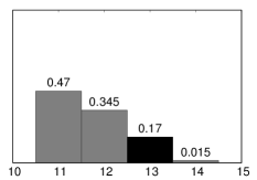
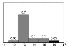
(a) $(128,13)$	(b) $(256,13)$	(c) $(512,16)$

Figure 2: Distribution of extracted maximum clique size, with black bars denoting the size of the planted clique. Both (a) and (b) are over 200 samples, while (c) is over 20 samples. In each, the predicting classifier has been trained with 64-vertex random graphs with a planted clique of size 10.

Table 2: Robustness and speedups with fixed $n$ and increasing $k$. The leftmost two columns show the data $(n,k)$ used to train a classifier $P$. For each planted clique size $k+1$, $k+2$, and $k+3$, we show the average pruning ratio (column “Pruned”), the average clique accuracy (column “Acc.’), the average runtime of igraph on the reduced instance obtained from our framework using $P$ (column “Time (s)”), and the average speedup over executing the same algorithm on the original instance.

			$k+1$				$k+2$				$k+3$
$n$	$k$	Pruned	Acc.	Time (s)	Speedup	Pruned	Acc.	Time (s)	Speedup	Pruned	Acc.	Time (s)	Speedup
64	10	0.530	0.905	0.068	0.132	0.548	0.965	0.068	0.135	0.564	0.995	0.068	0.135
128	12	0.506	0.710	0.301	0.759	0.517	0.875	0.296	0.774	0.525	0.935	0.297	0.784
256	13	0.489	0.170	3.261	3.264	0.493	0.190	3.233	3.304	0.493	0.310	3.260	3.315
512	15	0.492	0.05	70.587	12.994	0.492	0.05	70.086	12.816	0.491	0.100	70.562	12.722

Vertex classification accuracy

We study the accuracy of our classifiers for distinguishing vertices that are and are not in a maximum clique. Specifically, we train a classifier for each pair $(n,k)\in\{(64,10),(128,12),(256,12)\}$, and test for unseen graphs with the same $n$ but growing planted clique size $k^{\prime}=k+1,\ldots,k+4$. The results are shown in Figure 1 (a). As expected, the classification task becomes easier once $k^{\prime}$ increases. This is also supported the fact that multiple algorithms solve the planted clique problem in polynomial-time for large enough $k^{\prime}$ (see Subsection 5.1). In addition, as $n$ grows larger, we see accuracy deterioration caused by the converge of the local properties towards their expected values. Especially for small values of $k^{\prime}$, the injection of the planted clique is not substantial enough to cause significant deviations from the expected values.

Pruning ratio and clique accuracy

We study the effectiveness of our framework as a probabilistic preprocessor for the planted clique instances. We fix the confidence threshold $q=0.55$ and use the same set of classifiers and test data. The average pruning ratios over all instances are shown in Figure 1 (b). We see pruning ratios as high as at most 0.6, while always discarding more than 40 % of the vertices.

Now, it is possible that $P$ makes an erroneous prediction causing the deletion of a vertex, which in turn lowers the size of a maximum clique in the instance (although recall that this was not observed in Section 4 for real-world networks). The average clique accuracies over all instances are shown in Figure 1 (c). Here, we see that for $n=256$, the vertex accuracy (Figure 1 (a)) is still above 0.7, but the clique accuracy drops to above 0.4. As the vertex accuracy decreases, the probability of deleting a vertex present in a maximum clique increases, translating to a higher chance of error in extracting a maximum clique. However, while not completely error-free, we observe that even in the case of $(256,13)$ we always delete at most two members of a maximum clique, whereas in the case of $(512,16)$, 95 % of the time, we extract a maximum clique of size at least 13 (see Figure 2).

Robustness and speedups

The robustness and speedups obtained using the igraph algorithm are given in Table 2. Here, the clique accuracy and runtime are obtained as the average over 200 samples for each $(n,k)$ except for $(n,k)=(512,15)$ for which there are 20 independent samples. We see the drop in clique accuracy when a classifier $P$ is trained with $(n,k)\in\{(256,12),(512,15)\}$ and is predicting for the same $n$ but increasing $k$. The clique accuracy is a strict measure, so to quantify the severeness of the erroneous predictions made by $P$ we show the distributions of the extracted maximum clique sizes in Figure 2 for some pairs $(n,k)$. Again, we observe the effects of growing $n$ causing the convergence of local properties, consequently decreasing the predictive power of $P$. For $(n,k)=(128,13)$, 73 % of the runs still produce an optimal solution (here, one can also observe the rare event of having a maximum clique of size 14 when the planted clique was of size 13).

The case for supervised learning on intractable problems

Table 3: Deviation in vertex classification accuracy.

$n$	$k$	Trained acc.	Rob. acc.
128	12	0.858	0.844
256	13	0.747	0.728
512	15	0.678	0.665

As $n$ grows, the instances get increasingly time-consuming to solve even for state-of-the-art solvers for suitable $k$, as there is no exploitable structure. Consequently, obtaining optimally labeled data becomes practically impossible for large enough $n$. However, up to a point, random graphs with $n=64$ and $k=10$ are representative of the input for large graphs as well, and obtaining the optimal label for such a small graph is fast.

We show the deviation in vertex classification accuracy in Table 3. The column “Trained acc.” corresponds to the accuracy of the classifier trained with the values $n$ and $k$ mentioned in the two first columns, while the column “Rob. acc.” is the accuracy of a classifier trained with smaller $(n,k)=(64,10)$ instances, and predictions are made for the specified $(n,k)$ with planted clique size $k+1$. A key observation is that the difference between the two accuracies in a single row in Table 3 is small enough not to warrant training on larger instances. This offers an explanation for the perfect clique accuracy with limited training, as observed in Section 4 for real-world networks. This observation reduces the need of labeling costly data points for training.

6 Discussion and conclusions

We proposed a simple, powerful, and flexible machine learning framework for (i) reducing the search space of computationally difficult enumeration problems and (ii) augmenting existing state-of-the-art solvers with informative cues arising from the input distribution. In particular, we focused on a probabilistic preprocessing strategy, which retained all maximum cliques on a representative selection of large real-world networks from different domains. We showed the practicality of our framework by showing it speeds up the execution of state-of-the-art solvers on large graphs without compromising the solution quality. In addition, we demonstrated that supervised learning is a viable approach for tackling NP-hard problems in practice.

For future work, we will perform more extensive experiments on a wider set of instances, and provide a deeper analysis of our model.

References

- [Abu-Khzam et al. 2005] Abu-Khzam, F. N.; Baldwin, N. E.; Langston, M. A.; and Samatova, N. F. 2005. On the relative efficiency of maximal clique enumeration algorithms, with applications to high-throughput computational biology. In International Conference on Research Trends in Science and Technology.
- [Akkoyunlu 1973] Akkoyunlu, E. A. 1973. The enumeration of maximal cliques of large graphs. SIAM Journal of Computing 2(1):1–6.
- [Applegate et al. 2006] Applegate, D.; Bixby, R.; Chvátal, V.; and Cook, W. 2006. Concorde TSP solver.
- [Applegate et al. 2009] Applegate, D. L.; Bixby, R. E.; Chvátal, V.; Cook, W.; Espinoza, D. G.; Goycoolea, M.; and Helsgaun, K. 2009. Certification of an optimal TSP tour through 85,900 cities. Operations Research Letters 37(1):11–15.
- [Baldwin et al. 2004] Baldwin, N. E.; Collins, R. L.; Langston, M. A.; Leuze, M. R.; Symons, C. T.; and Voy, B. H. 2004. High performance computational tools for Motif discovery. In Parallel and Distributed Processing Symposium.
- [Bello et al. 2016] Bello, I.; Pham, H.; Le, Q. V.; Norouzi, M.; and Bengio, S. 2016. Neural combinatorial optimization with reinforcement learning. arXiv preprint arXiv:1611.09940.
- [Bernard, Killworth, and Sailer 1979] Bernard, H. R.; Killworth, P. D.; and Sailer, L. 1979. Informant accuracy in social network data iv: a comparison of clique-level structure in behavioral and cognitive network data. Social Networks 2(3):191–218.
- [Boginski, Butenko, and Pardalos 2005] Boginski, V.; Butenko, S.; and Pardalos, P. M. 2005. Statistical analysis of financial networks. Computational Statistics and Data Analysis 48(2):431–443.
- [Bollobás 2013] Bollobás, B. 2013. Modern graph theory, volume 184. Springer Science & Business Media.
- [Bomze et al. 1999] Bomze, I.; Budinich, M.; Pardalos, P.; and Pelillo, M. 1999. The Maximum Clique Problem. In Handbook of Combinatorial Optimization, volume 4. Kluwer Academic Publishers. 1–74.
- [Bron and Kerbosch 1973] Bron, C., and Kerbosch, J. 1973. Algorithm 457: finding all cliques of an undirected graph. Communications of the ACM 16(9):575–577.
- [Bruck and Goodman 1988] Bruck, J., and Goodman, J. W. 1988. On the power of neural networks for solving hard problems. In Neural Information Processing Systems, 137–143.
- [Buló, Torsello, and Pelillo 2009] Buló, S. R.; Torsello, A.; and Pelillo, M. 2009. A game-theoretic approach to partial clique enumeration. Image and Vision Computing 27(7).
- [Cazals and Karande 2008] Cazals, F., and Karande, C. 2008. A note on the problem of reporting maximal cliques. Theoretical Computer Science 407:564–568.
- [Chen et al. 2006] Chen, J.; Huang, X.; Kanj, I. A.; and Xia, G. 2006. Strong computational lower bounds via parameterized complexity. Journal of Computer and System Sciences 72(8):1346–1367.
- [Cheng et al. 2011] Cheng, J.; Ke, Y.; Fu, A. W.-C.; Yu, J. X.; and Zhu, L. 2011. Finding maximal cliques in massive networks. ACM Transactions on Database Systems (TODS) 36(4):21.
- [Cheng et al. 2012] Cheng, J.; Zhu, L.; Ke, Y.; and Chu, S. 2012. Fast Algorithms for Maximal Clique Enumeration with Limited Memory. In KDD, 1240–1248.
- [Csardi and Nepusz 2006] Csardi, G., and Nepusz, T. 2006. The igraph software package for complex network research. InterJournal Complex Systems:1695.
- [Devlin and O’Sullivan 2008] Devlin, D., and O’Sullivan, B. 2008. Satisfiability as a classification problem. In Proc. of the 19th Irish Conf. on Artificial Intelligence and Cognitive Science.
- [Durbin and Willshaw 1987] Durbin, R., and Willshaw, D. 1987. An analogue approach to the travelling salesman problem using an elastic net method. Nature 326(6114):689.
- [Dutta, Nayek, and Bhattacharya 2017] Dutta, S.; Nayek, P.; and Bhattacharya, A. 2017. Neighbor-Aware Search for Approximate Labeled Graph Matching using the Chi-Square Statistics. In International Conference on World Wide Web (WWW), 1281–1290.
- [Eblen et al. 2012] Eblen, J. D.; Phillips, C. A.; Rogers, G. L.; and Langston, M. A. 2012. The maximum clique enumeration problem: algorithms, applications, and implementations. In BMC bioinformatics, volume 13, S5. BioMed Central.
- [Eppstein, Löffler, and Strash 2010] Eppstein, D.; Löffler, M.; and Strash, D. 2010. Listing all maximal cliques in sparse graphs in near-optimal time. In International Symposium on Algorithms and Computation (ISAAC), 403–414.
- [Erdös and Rényi 1959] Erdös, P., and Rényi, A. 1959. On random graphs, I. Publicationes Mathematicae (Debrecen) 6:290–297.
- [Faust and Wasserman 1995] Faust, K., and Wasserman, S. 1995. Social network analysis: Methods and applications. Cambridge University Press.
- [Feldman et al. 2017] Feldman, V.; Grigorescu, E.; Reyzin, L.; Vempala, S. S.; and Xiao, Y. 2017. Statistical algorithms and a lower bound for detecting planted cliques. Journal of the ACM 64(2):8:1–8:37.
- [Feurer et al. 2015] Feurer, M.; Klein, A.; Eggensperger, K.; Springenberg, J.; Blum, M.; and Hutter, F. 2015. Efficient and robust automated machine learning. In Advances in Neural Information Processing Systems (NIPS). 2962–2970.
- [Fitzgerald, Malitsky, and O’Sullivan 2015] Fitzgerald, T.; Malitsky, Y.; and O’Sullivan, B. 2015. ReACTR: Realtime Algorithm Configuration through Tournament Rankings. In IJCAI, 304–310.
- [Fort 1988] Fort, J. C. 1988. Solving a combinatorial problem via self-organizing process: An application of the Kohonen algorithm to the traveling salesman problem. Biological Cybernetics 59(1):33–40.
- [Gomes et al. 2000] Gomes, C. P.; Selman, B.; Crato, N.; and Kautz, H. 2000. Heavy-tailed phenomena in satisfiability and constraint satisfaction problems. Journal of Automated Reasoning 24(1-2):67–100.
- [Gomes, Selman, and Kautz 1998] Gomes, C. P.; Selman, B.; and Kautz, H. 1998. Boosting combinatorial search through randomization. AAAI/IAAI 98:431–437.
- [He, Daume III, and Eisner 2014] He, H.; Daume III, H.; and Eisner, J. M. 2014. Learning to search in branch and bound algorithms. In Advances in Neural Information Processing Systems (NIPS), 3293–3301.
- [Hopfield and Tank 1985] Hopfield, J. J., and Tank, D. W. 1985. “Neural” computation of decisions in optimization problems. Biological cybernetics 52(3):141–152.
- [Hutter et al. 2009] Hutter, F.; Hoos, H. H.; Leyton-Brown, K.; and Stützle, T. 2009. ParamILS: an automatic algorithm configuration framework. Journal of Artificial Intelligence Research 36:267–306.
- [Jerrum 1992] Jerrum, M. 1992. Large cliques elude the Metropolis process. Random Structures & Algorithms 3(4):347–359.
- [Karp 1976] Karp, R. M. 1976. The probabilistic analysis of some combinatorial search algorithms. Algorithms and complexity: New directions and recent results 1:19.
- [Khalil et al. 2016] Khalil, E. B.; Le Bodic, P.; Song, L.; Nemhauser, G. L.; and Dilkina, B. N. 2016. Learning to branch in mixed integer programming. In AAAI, 724–731.
- [Khalil et al. 2017] Khalil, E.; Dai, H.; Zhang, Y.; Dilkina, B.; and Song, L. 2017. Learning combinatorial optimization algorithms over graphs. In Advances in Neural Information Processing Systems, 6351–6361.
- [Kose et al. 2001] Kose, F.; Weckwerth, W.; Linke, T.; and Fiehn, O. 2001. Visualizing plant metabolomic correlation networks using clique-metabolite matrices. Bioinformatics 17(12):1198–1208.
- [Kučera 1995] Kučera, L. 1995. Expected complexity of graph partitioning problems. Discrete Applied Mathematics 57(2):193–212.
- [Li, Jiang, and Manyà 2017] Li, C.-M.; Jiang, H.; and Manyà, F. 2017. On minimization of the number of branches in branch-and-bound algorithms for the maximum clique problem. Computers & Operations Research 84:1–15.
- [Liang et al. 2016] Liang, J. H.; Ganesh, V.; Poupart, P.; and Czarnecki, K. 2016. Learning rate based branching heuristic for SAT solvers. In International Conference on Theory and Applications of Satisfiability Testing, 123–140. Springer.
- [Loreggia et al. 2016] Loreggia, A.; Malitsky, Y.; Samulowitz, H.; and Saraswat, V. A. 2016. Deep learning for algorithm portfolios. In AAAI, 1280–1286.
- [McKay and Piperno 2014] McKay, B. D., and Piperno, A. 2014. Practical graph isomorphism, II. Journal of Symbolic Computation 60(0):94–112.
- [Modani and Dey 2008] Modani, N., and Dey, K. 2008. Large maximal cliques enumeration in sparse graphs. In CIKM, 1377–1378.
- [Niskanen and Östergård 2003] Niskanen, S., and Östergård, P. R. 2003. Cliquer User’s Guide: Version 1.0. Helsinki University of Technology Helsinki, Finland.
- [Nowak et al. 2017] Nowak, A.; Villar, S.; Bandeira, A. S.; and Bruna, J. 2017. A note on learning algorithms for quadratic assignment with graph neural networks. arXiv preprint arXiv:1706.07450.
- [Östergård 2002] Östergård, P. R. 2002. A fast algorithm for the maximum clique problem. Discrete Applied Mathematics 120(1):197–207.
- [Pattabiraman et al. 2013] Pattabiraman, B.; Patwary, M. M. A.; Gebremedhin, A. H.; Liao, W.-k.; and Choudhary, A. 2013. Fast algorithms for the maximum clique problem on massive sparse graphs. In Algorithms and Models for the Web Graph (WAW), 156–169.
- [Pedregosa et al. 2011] Pedregosa, F.; Varoquaux, G.; Gramfort, A.; Michel, V.; Thirion, B.; Grisel, O.; Blondel, M.; Prettenhofer, P.; Weiss, R.; Dubourg, V.; Vanderplas, J.; Passos, A.; Cournapeau, D.; Brucher, M.; Perrot, M.; and Duchesnay, E. 2011. Scikit-learn: Machine learning in Python. Journal of Machine Learning Research 12:2825–2830.
- [Read and Cressie 1988] Read, T. R. C., and Cressie, N. A. C. 1988. Goodness-of-fit statistics for discrete multivariate data. Springer.
- [Read and Cressie 1989] Read, T., and Cressie, N. 1989. Pearson’s and the likelihood ratio statistic : a comparative review. International Statistical Review 57(1):19–43.
- [Rossi and Ahmed 2015] Rossi, R. A., and Ahmed, N. K. 2015. The network data repository with interactive graph analytics and visualization. In AAAI.
- [Schmidt et al. 2009] Schmidt, M. C.; Samatova, N. F.; Thomas, K.; and Park, B. H. 2009. A scalable, parallel algorithm for maximal clique enumeration. Journal of Parallel Distributed Computing 69(4):417–428.
- [Stix 2004] Stix, V. 2004. Finding all maximal cliques in dynamic graphs. Computational Optimization and applications 27:173–186.
- [Tomita, Tanaka, and Takahashi 2006] Tomita, E.; Tanaka, A.; and Takahashi, H. 2006. The worst-case time complexity for generating all maximal cliques and computational experiments. Theoretical Computer Science 363(1):28–42.
- [Vinyals, Fortunato, and Jaitly 2015] Vinyals, O.; Fortunato, M.; and Jaitly, N. 2015. Pointer networks. In Advances in Neural Information Processing Systems (NIPS), 2692–2700.
- [Wan et al. 2006] Wan, L.; Wu, B.; Du, N.; Ye, Q.; and Chen., P. 2006. A new algorithm for enumerating all maximal cliques in complex network. In ADMA, 606–617.
- [Watts and Strogatz 1998] Watts, D. J., and Strogatz, S. H. 1998. Collective dynamics of ‘small-world’ networks. Nature 393(6684):440.
- [Wu et al. 2009] Wu, B.; Yang, S.; Zhao, H.; and Wang, B. 2009. A distributed algorithm to enumerate all maximal cliques in MapReduce. In International Conference on Frontier of Computer Science and Technology, 45–51.
- [Xu, Koenig, and Kumar 2018] Xu, H.; Koenig, S.; and Kumar, T. S. 2018. Towards effective deep learning for constraint satisfaction problems. In International Conference on Principles and Practice of Constraint Programming, 588–597. Springer.
- [Yao 1992] Yao, X. 1992. Finding approximate solutions to NP-hard problems by neural networks is hard. Information Processing Letters 41(2):93–98.
- [Yeger-Lotem et al. 2004] Yeger-Lotem, E.; Sattath, S.; Kashtan, N.; Itzkovitz, S.; Milo, R.; Pinter, R. Y.; Alon, U.; and Margalit, H. 2004. Network motifs in integrated cellular networks of transcription–regulation and protein–protein interaction. Proceedings of the National Academy of Sciences of the United States of America 101(16):5934–5939.
- [Zhang et al. 2005] Zhang, Y.; Abu-Khzam, F. N.; Baldwin, N. E.; Chesler, E. J.; Langston, M. A.; and Samatova, N. F. 2005. Genome-scale computational approaches to memory-intensive applications in systems biology. In Supercomputing.
- [Zuckerman 2006] Zuckerman, D. 2006. Linear degree extractors and the inapproximability of max clique and chromatic number. In Proceedings of the 38th Annual ACM Symposium on Theory of Computing (STOC), 681–690. ACM.