A Double-station Access Protocol for Optical Wireless Scattering Communication Networks

Abstract

We propose a double-station access protocol (DS-CSMA) with multiple backoff mechanism for optical wireless scattering communication networks (OWSCN). Furthermore, we extend existing Bianchi Markov model into state transmission model to analyze the collision probability, throughput and average delay. For the application of protocol, we propose to optimize the initial contention window and indicator matrix to maximize throughput. Both numerical and simulation results imply that the proposed protocol can achieve higher throughput and lower transmission delay compared with state-of-art baseline.

I Introduction

Optical wireless scattering communication (OWSC) can potentially offer high data rate transmission due to its large bandwidth [1, 2]. Without emitting or being negatively affected by electromagnetic radiation, it can be applied to many scenarios where conventional radio-frequency (RF) communication is prohibited, for instance in the battlefield where radio silence is required [3]. Various physical layer techniques has been proposed as the foundation of optical wireless scattering communication networks (OWSCN), including the multi-user signal detection [4, 5], information security [6], neighbor discovery [7] and error correction codes [8].

Different from RF-based communication networks, the received signal of OWSC exhibits the characteristics of discrete photoelectrons due to the extremely large path loss [9]. Hence, Poisson-type channel model has been adopted for photon-counting-based physical-layer signal processing [10, 11]. Network communication for OWSC has been studied in existing works [12]. Specifically, a cluster-based algorithm has been proposed in [7] for neighbour discovery; the achievable rates of multiple access users have been addressed in [4]; and a count-and-forward protocol has been proposed in [13]. Furthermore, according to [14, 15], the authors proposed a superimposed transmission for OWSC, where different users are assigned into different signal layers so that the overall symbol rate doubles without reducing the symbol duration, and investigated the physical-layer techniques of transmission such as channel parameter estimation, signal detection and decoding.

As a classical medium access control (MAC) protocol, Carrier Sense Multiple Access (CSMA) is a widely adopted in wireless networks and leads to many improved versions [16]. One typical method is to combine Carrier Sense Multiple Access with Collision Avoidance (CSMA/CA) with multi-packet reception (MPR) [17]. Specifically, MPR protocol employs CSMA/CA protocol and Request To Send/Clear To Send (RTS/CTS) mechanism for medium access control, and introduces Code Devision Multiple Access(CDMA) or Orthogonal Frequency Division Multiple Access (OFDMA) to transmit multiple data packages [18]. It allows higher throughput transmission than the conventional CSMA and gradually leads to many advanced versions which can be applied in different scenarios, such as MPR with random access [19], acknowledgment-aware asynchronous patterns [20] and adaptive Backoff Algorithm [21].

Even through MPR enables higher throughput by employing CDMA or OFDMA into the protocol, the overall throughput is still limited by the single backoff mechanism of conventional CSMA/CA. In this work, we discover that multiple backoff mechanism results in higher throughput than the conventional single backoff mechanism in CSMA, and propose double-station CSMA (DS-CSMA) protocol for OWSCN. Different from MPR, without depending on CDMA, OFDMA or other orthogonal multi-user communication, we adopts superimposed transmission [15] to deal with the packages from double stations in the physical-layer, where channel estimation, synchronization, joint detection and decoding have been investigated in [14].

Such MAC protocol with multiple backoff mechanism and superimposed transmission has not been addressed for radio-frequency wireless communication yet. Specifically, as shown in Figure 1, each station employs multiple time counter to execute backoff processes. Any two time counters (marked with the same color) are regarded as a pair, and one of the time counter backoff to 0 can trigger the pairs’ superimposed transmission. Such multiple backoff mechanism is more flexible than conventional single backoff mechanism in maximizing overall throughput and reducing transmission delay.

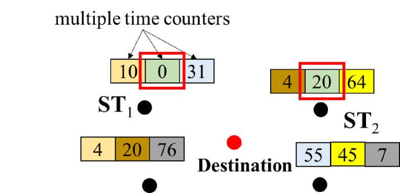
(a) Time counter $(2,1)$ backoff to zeros.

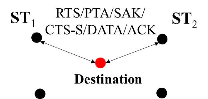
(b) Superimposed transmission from stations 1 and 2.

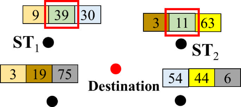
(c) Time counters $(2,1)$ and $(1,2)$ randomly take new values for next backoff.

Figure 1: Multiple backoff mechanism: Each station employs multiple backoff process to strive for the chance of data transmission. Each lattice represents a time counter to execute the backoff process; 2 lattices with the same color implies the 2 stations will have superimposed transmission when backoff to 0; Time counter $(i,j)$ means time counter $i$ of station $j$.

On the other hand, Bianchi Model (based on discrete Markov model) has been widely applied in throughput analysis for various types of MAC protocol, e.g. [18, 20, 22]. However, existing works on Bianchi Model cannot be directly applied to our proposed DS-CSMA protocol, since the state transition depends on more than one stations. Hence, we extend Bianchi Model to the state transition model considered in this work, and obtain the numerical solutions to the throughput and collision probability. Such numerical results are validated by simulation results. Furthermore, we propose to approximately maximize the throughput with respect to the initial contention window and indicator matrix. Numerical results demonstrate that the proposed protocol with optimized parameters can significantly outperform CSMA-based MAC including that with MPR.

The remainder of this paper is organized as follows. In Section II, we introduce the indicator matrix and specify the DS-CSMA protocol. In Sections III and IV, we provide a state transition model to analyze the collision probability and throughput. In Section V, we propose to optimize the initial contention window and indicator matrix to maximize throughput. Numerical and simulation results are shown in Section VI to evaluate the performance of DS-CSMA protocol, and the comparison with conventional CSMA including that with MPR. Finally, Section VII concludes this work.

II Double Station CSMA Protocol with Multiple Backoff Mechanism

II-A Superimposed Frame Detection with Symbol Boundary Misalignment for OWSCN

We consider an OWSCN consisting of $N_{s}$ active stations, where multiple stations can transmit packages to a common destination (only single destination is considered in this work). Since different stations’ transmissions can be performed in asynchronous patterns and interfere with each other, the frames can be superimposed with symbol boundary misalignment, where the relative delays are within one symbol duration. The achievable rate and frame detection for the superimposed transmission have been investigated in [14, 15], which can be adopted as the physical-layer technique to transmit data frames from two stations considered in this work. In this work, we propose a double-station access protocol based on CSMA/CA that can utilize the joint detection of superposed signal from two different stations.

In the protocol, each station $i$ deploys $J_{i}$ independent time counters $T_{i,1},T_{i,2},\cdots,T_{i,J_{i}}$ to control the packet transmission. For the convenience of specification, we define the following two important terms and other notations in Table I.

• Time counter pair (TCPair): The two time counters in two stations that can transmit simultaneously with signal superposition at the receiver.

• Partner time counter (PTCounter): Within a TCPair, the two time counters are PTCounter of each other.

II-B Indicator matrix

An indicator matrix $\boldsymbol{\Phi}$ is assumed known for the destination to reserve all indices of TCPairs, where $\boldsymbol{\Phi}=[\phi_{i,j}|1\leq i\leq N_{s},1\leq j\leq N_{s}]$ is a zero-one matrix depending on the link gains in the physical layer. We let $J_{i}=\sum^{N_{s}}_{k=1}\phi_{i,k}$ denote the number of PTCounters with station $i$, and $N$ denote the total number of TCPairs in the networks, where $N=\frac{1}{2}\sum_{i=1}^{N_{s}}J_{i}=\frac{1}{2}\sum_{i=1}^{N_{s}}\sum_{i^{\prime}=0}^{N_{s}}\phi_{i,i^{\prime}}$. We use $\phi_{i,i^{\prime}}=1$ to indicate that stations $i$ and $i^{\prime}$ can have a superimposed transmission of data frames controlled by TCPair $(T_{i,j},T_{i^{\prime},j^{\prime}})$, where $j=\sum^{i^{\prime}}_{k=1}\phi_{i,k}$ and $j^{\prime}=\sum^{i}_{k=1}\phi_{i^{\prime},k}$; $\boldsymbol{\Phi}$ is symmetrical and $\phi_{i,i}=0$ since TCPairs $(T_{i,j},T_{i^{\prime},j^{\prime}})$ and $(T_{i^{\prime},j^{\prime}},T_{i,j})$ must coexist for $i\neq i^{\prime}$. An example is that

$$\boldsymbol{\Phi}=\left[\begin{smallmatrix}0&1&0&1&1\\ 1&0&1&1&1\\ 0&1&0&1&1\\ 1&1&1&0&0\\ 1&1&1&0&0\end{smallmatrix}\right],$$ (1)

where $\phi_{1,2}=\phi_{2,1}=1$ indicates $T_{1,1}$ of station 1 and $T_{2,1}$ of station 2 can form TCPair $(T_{1,1},T_{2,1})$; and $T_{1,1}$ and $T_{2,1}$ are PTCounters of each other.

II-C Channel Contention with Multiple Backoff Mechanism

Before transmission, the initial values of all time counters $T_{i,j}$ for $1\leq i\leq N_{s},1\leq j\leq J_{i}$ are uniformly chosen from $[0,W_{i,j}-1]$, where $W_{i,j}$ denotes the contention window of $T_{i,j}$. A common minimum and maximum contention window $W_{0}$ and $W_{\max}$ are shared by all time counters.

TABLE I: Specification of notations.

	Notation	Denotation
OWSCN	$N_{s}$	Number of stations
	$\boldsymbol{\Phi}$	Indicator matrix
	$N$	Number of TCPairs
Station $i$	$J_{i}$	Number of time counters
	$T_{i,1},T_{i,2},\cdots,T_{i,J_{i}}$	Time counters
	$W_{i,1},W_{i,2},\cdots,W_{i,J_{i}}$	Current contention window
	$W_{0}$	Minimum contention window
	$W_{\max}$	Maximum contention window

For each time counter $T_{i,j}$, $W_{i,j}$ is selected as $2^{m_{i,j}}W_{0}$, where $m_{i,j}$ takes from $0,1,2,\cdots,M-1$ with $W_{\max}=2^{M-1}W_{0}$. Furthermore, the time counters are decremented as long as the channel is sensed idle, as the backoff process in the CSMA/CA protrocol, and keep unchanged when the channel is sensed busy. More specifically, the proposed protocol is characterized into the following $3$ parts.

• Once a time counter $T_{i,j}$ of station $i$ decreases to $0$, its backoff process is stopped, and station $i$ conducts the following active transmission:

  • It sends the RTS frame (request to send frame) to the destination, which contains its 2-dimensional index $(i,j)$, as shown in Figure 2.4., and waits for the PTA frame (partner activate) from the destination.

  • Once receiving the PTA frame, it waits for the CTS-S frame (clear to send-superimposed transmission) from the destination. In case of missing the PTA frame (waiting for the period of PTA frame but failing to receive the PTA frame), it doubles the contention window of $T_{i,j}$ by updating $W_{i,j}\leftarrow 2W_{i,j}$, as shown in Figure 2.8., and jump to step 1e).

  • After receiving the CTS-S, it transmits data frame to the destination, as shown in Figure 2.14., and waits for ACK (acknowledgement) from the destination.

  • On receiving the ACK, it resets the contention window of $T_{i,j}$ to $W_{0}$, i.e., $W_{i,j}\leftarrow W_{0}$.

  • Randomly choose an integer from $[0,W_{i,j}-1]$ for $T_{i,j}$ as its initial backoff value, and restarts the backoff process in a DIFS. Other time counters also reactive their previous backoff process in a DIFS.

• Once the destination receives the RTS frame from a certain station with the 2-dimensional index $(i,j)$ of $T_{i,j}$, it obtains the index $(i^{\prime},j^{\prime})$ of PTCounter $T_{i^{\prime},j^{\prime}}$ according to the indicator matrix $\boldsymbol{\Phi}$, and manages to receive data frames from stations $i$ and $i^{\prime}$ into the following steps:

  • It broadcasts the PTA frame containing $(i^{\prime},j^{\prime})$ to all stations, and waits for the SAK (superposition acknowledgement) from station $i^{\prime}$.

  • Once receiving the SAK, it broadcasts the CTS-S frame to stations $i$ and $i^{\prime}$, as shown in Figure 3, and waits for the superimposed data transmission.

  • After successfully decoding the superimposed data frames, it broadcasts the ACK to all stations.

• For station $\tilde{i}\neq i^{\prime}$, upon receiving the PTA frame from the destination, its time counters stop backoff process such that the channel is available for stations $i$ and $i^{\prime}$. Once receiving the ACK from the destination, its time counters reactive their previous backoff process in a DIFS. For station $i^{\prime}$, upon receiving the PTA frame from the destination, its time counters stop the backoff process, and conducts the transmission via the following steps:

  • As shown in Figure 2.12., it transmits the SAK frame to the destination, which contains whether it will have a superimposed transmission with station $i$. In case of refusing to have superimposed transmission with station $i$, it jump to 3d).

  • After transmitting the SAK frame, it waits for the CTS-S frame from the destination.

  • Upon receiving the CTS-S frame, without having to cooperate with station $i$, it transmits data frame as soon as possible, as shown in Figure 2.14., and waits for the ACK from the destination.

  • Once receiving the ACK, $T_{i^{\prime},j^{\prime}}$ resets the contention window to $W_{0}$, randomly chooses a value from $[0,W_{0}-1]$ as its initial backoff value, and restarts the backoff process in a DIFS. Other time counters also reactive their previous backoff process in a DIFS.

For clarification, we summarize all types of control frames in Table II. A successful superimposed transmission of data frames consists of the exchanges of RTS, PTA, SAK, CTS, Data and ACK frames, as shown in Figure 3. A collision happens when more than one stations transmits RTSs to the destination simultaneously.

TABLE II: Specification of different type of frames.

Frame type	Function
RTS	Ask for occupying the common channel
PTA	Activate the PTCounter and freeze other TCPairs
SAK	Acknowledgement of a superimposed transmission
CTS-S	Clear to send-superimposed transmission
ACK	Flag of a complete superimposed transmission

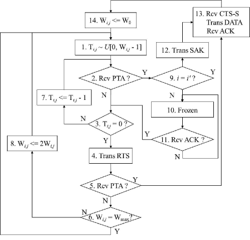
Figure 2: Flowchart of DS-CSMA protocol.

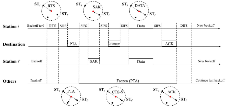
Figure 3: Frame sequence of a successful superimposed transmission.

II-D An Example of DS-CSMA

We give an example on the proposed DS-CSMA protocol in this subsection. We assume $5$ stations with the indicator matrix in Equation (1), where $8$ TCPairs are deployed to control data transmission. Provided that $W_{i,j}=W_{0}=32$ and $W_{\max}=128$, the states of $8$ TCPairs at certain time point are shown in the first column of Table III.

After $3$ time slots, the TCPairs are illustrated in the second column of Table III, where $T_{1,2}$ and $T_{4,3}$ are both reduced to $0$. Accordingly, stations $1$ and $4$ both transmit the RTS-S frame to the destination, where a collision happens. Then, they conduct steps 1a), 1b) and 1e). The new initial backoff values are chosen from $[0,64]$, e.g., $T_{1,2}=26,T_{4,3}=58$.

After another $2$ time slots, the TCPairs are self-decrement twice and turn to the states shown in the third column of Table III, where only $T_{3,2}$ is reduced to $0$. Therefore, stations $3$ and $4$ conduct a successful superimposed transmission as shown in Figure 3, where station $3$ conducts steps 1a)-1e); and station $4$ conducts steps 3a)-3d).

TABLE III: Example of DS-CSMA.

Initial	$3$ time slots later	$5$ time slots later
$(T_{1,1},T_{2,1})=(3,28)$ $(T_{1,2},T_{4,1})=(19,13)$ $(T_{1,3},T_{5,1})=(8,30)$ $(T_{2,2},T_{3,1})=(24,6)$ $(T_{2,3},T_{4,2})=(9,31)$ $(T_{2,4},T_{5,2})=(11,17)$ $(T_{3,2},T_{4,3})=(5,33)$ $(T_{3,3},T_{5,3})=(29,7)$	$(T_{1,1},T_{2,1})=(0,25)$ $(T_{1,2},T_{4,1})=(16,10)$ $(T_{1,3},T_{5,1})=(5,27)$ $(T_{2,2},T_{3,1})=(21,3)$ $(T_{2,3},T_{4,2})=(6,28)$ $(T_{2,4},T_{5,2})=(8,14)$ $(T_{3,2},T_{4,3})=(2,0)$ $(T_{3,3},T_{5,3})=(26,4)$	$(T_{1,1},T_{2,1})=(24,23)$ $(T_{1,2},T_{4,1})=(14,8)$ $(T_{1,3},T_{5,1})=(3,25)$ $(T_{2,2},T_{3,1})=(19,1)$ $(T_{2,3},T_{4,2})=(4,26)$ $(T_{2,4},T_{5,2})=(6,12)$ $(T_{3,2},T_{4,3})=(0,56)$ $(T_{3,3},T_{5,3})=(24,2)$

III State Transition Model for DS-CSMA

Conventional theories (Bianchi Model) [22] of throughput analysis for distributed CSMA/CA cannot be directly applied to our proposed DS-CSMA protocol since each station depends on more than one time counters. To address this issue, we choose to use state $(T_{i_{1},j_{1}},T_{i_{2},j_{2}})$ to characterize a TCPair. For simplicity but without loss of generality, we consider the state transition of certain TCPair as the representation of whole system. The subscript of time counters $(T_{i_{1},j_{1}},T_{i_{2},j_{2}})$ can be simplified into $(T_{1},T_{2})$ characterized by parameters $(m,n,i,j)$, where $m$ and $n$ denote that the contention windows of the $T_{1}$ and $T_{2}$ equal $W_{m}=2^{m}W_{0}$ and $W_{n}=2^{n}W_{0}$, respectively; and $i$ and $j$ notate that $(T_{1},T_{2})=(i,j)$. Furthermore, let $\mathbb{P}(m,n,i,j)$ denote the probability of state $(m,n,i,j)$, and $\mathbb{P}(m,n,i,j|m^{\prime},n^{\prime},i^{\prime},j^{\prime})$ denote the state transition probability from state $(m^{\prime},n^{\prime},i^{\prime},j^{\prime})$ to state $(m,n,i,j)$, where $0\leq m,m^{\prime},n,n^{\prime}\leq M-1,0\leq i,i^{\prime}\leq W_{m}-1,0\leq j,j^{\prime}\leq W_{n}-1$.

III-A State Transition Probabilities

First of all, for $0\leq i\leq W_{m}-1,0\leq j\leq W_{n}-1$, both $T_{1}$ and $T_{2}$ must be reduced by one in the next slot. Hence the transition probability is given by

$$\mathbb{P}(m,n,i,j|m,n,i+1,j+1)=1.$$ (2)

The remaining cases depend on parameter $p$, the probability that a collision happens in the channel due to other TCPairs’ contention. Probability $p$ is determined by parameters $N$ and $\eta$ as follows,

$$p=1-(1-\eta)^{N-1},$$ (3)

where $N=\frac{1}{2}\sum_{i=1}^{N_{s}}\sum_{j=1}^{N_{s}}\phi_{i,j}$ denotes the number of TCPairs as shown in Table I; and

$$\eta=\sum_{m=0}^{M-1}\sum_{n=0}^{M-1}\Big{[}\sum_{i=1}^{W_{m}-1}\mathbb{P}(m,n,i,0)+\sum_{j=1}^{W_{n}-1}\mathbb{P}(m,n,0,j)\Big{]}$$ (4)

denotes the overall probability that one of the time counters is reduced to $0$.

Secondly, for $i=0$ or $j=0$, it will lead to two cases of state-transmission. A new successful transmission, consisting of RTS, PTA, SAK, CTS, Data frame superimposed transmission and ACK, may happen with probability $(1-p)$. After a successful transmission, $T_{1}$ and $T_{2}$ are independently initialized uniformly in the range $[0,W_{0}-1]$. Accordingly, the transition probabilities are given by

$$\mathbb{P}(0,0,i,j|m,n,i^{\prime},0)=\frac{1-p}{W_{0}^{2}},\quad\mathbb{P}(0,0,i,j|m,n,0,j^{\prime})=\frac{1-p}{W_{0}^{2}}.$$ (5)

Besides, the RTS-S may collide with that from other stations with probability $p$. In this case, if $m,n\neq M-1$, either $T_{1}$ or $T_{2}$ may be uniformly chosen in range $[0,W_{m+1}-1]$ or $[0,W_{n+1}-1]$ with probability $p$, and thus the transition probabilities are given by

$$\mathbb{P}(m+1,n,i,j|m,n,0,j+1)=\frac{p}{W_{m+1}},\quad\mathbb{P}(m,n+1,i,j|m,n,i+1,0)=\frac{p}{W_{n+1}}.$$ (6)

Furthermore, if $m=M-1$ or $n=M-1$, the contention windows of either $T_{1}$ or $T_{2}$ will never become doubled in subsequent transmission, and the transition probabilities are given by

$$\mathbb{P}(M-1,n,i,j|M-1,n,0,j+1)=\mathbb{P}(m,M-1,i,j|m,M-1,i+1,0)=\frac{p}{W_{M-1}}.$$ (7)

In addition, if $m=n=M-1$, neither $T_{1}$ or $T_{2}$ will be doubled the contention window in subsequent transmissions. Hence, the transition probabilities are given by

$$\mathbb{P}(M-1,M-1,i,j|M-1,M-1,0,j+1)=\mathbb{P}(M-1,M-1,i,j|M-1,M-1,i+1,0)=\frac{p}{W_{M-1}}.$$ (8)

Finally, considering $i=j=0$, where $T_{1}$ and $T_{2}$ decrease to $0$ simultaneously, where a collision must happen. For $m,n\neq M-1$, $T_{1}$ and $T_{2}$ will uniformly take values in $[0,W_{m+1}-1]$ and $[0,W_{n+1}-1]$, respectively. The transition probability is given by

$$\mathbb{P}(m+1,n+1,i,j|m,n,0,0)=\frac{1}{W_{m+1}W_{n+1}}.$$ (9)

For $m=M-1$ or $n=M-1$, either $W_{m}$ or $W_{n}$ is never doubled since it is up to the maximum contention window $W_{\max}$. Then, the transition probabilities are given by,

$$\mathbb{P}(M-1,n+1,i,j|M-1,n,0,0) =\frac{1}{W_{M-1}W_{n+1}},$$ (10)

$$\mathbb{P}(m+1,M-1,i,j|m,M-1,0,0) =\frac{1}{W_{m+1}W_{M-1}}.$$

For $m=n=M-1$, neither $W_{m}$ or $W_{n}$ will be doubled, and the transition probabilities are given by

$$\mathbb{P}(M-1,M-1,i,j|M-1,M-1,0,0)=\frac{1}{W_{M-1}^{2}}.$$ (11)

III-B The State Probabilities

We obtain the state probabilities in this subsection based on the state transition probabilities. Since $i$ and $j$ take values in $[0,W_{m}-1]$ and $[0,W_{n}-1]$, respectively, it is convinced that $\mathbb{P}(m,n,W_{m},\bullet)=\mathbb{P}(m,n,\bullet,W_{n})=\mathbb{P}(m,n,W_{m},W_{n})=0$ for $0\leq m,n\leq M-1$. We summarize all possible state probabilities into the following $7$ cases.

Case 1: For $m=n=0,0\leq i\leq W_{0}-1,0\leq j\leq W_{0}-1$, as shown in Figure 4(a), the previous states of $(0,0,i,j)$ are $(0,0,i+1,j+1)$, $(0,0,0,1),(0,0,0,2),\cdots,(M-1,M-1,0,W_{M-1}-1)$ as well as $(0,0,1,0),(0,0,2,0),\cdots,(M-1,M-1,W_{M-1}-1,0)$, and thus

$$\mathbb{P}(0,0,i,j)=\mathbb{P}(0,0,i+1,j+1)+\eta\frac{1-p}{W^{2}_{0}},$$ (12)

where $\eta$ is given by Equation (4).

Case 2: For $0<m<M-1,n=0,0\leq i\leq W_{m}-1,0\leq j\leq W_{0}-1$, as shown in Figure 4(b), the previous states of $(m,0,i,j)$ are $(m,0,i+1,j+1)$ as well as $(m-1,0,0,j+1)$, and thus

$$\mathbb{P}(m,0,i,j)=\mathbb{P}(m,0,i+1,j+1)+\frac{\mathbb{P}(m-1,0,0,j+1)}{W_{m}}p.$$ (13)

Case 3: For $m=M-1,n=0$, $0\leq i\leq W_{M-1}-1$ and $1\leq j\leq W_{0}-1$, as shown in Figure 4(c), the previous states of $(M-1,0,i,j)$ are $(M-1,0,i+1,j+1)$, $(M-2,0,0,j+1)$ as well as $(M-1,0,0,j+1)$, and thus

$$\mathbb{P}(M-1,0,i,j)=\mathbb{P}(M-1,0,i+1,j+1)+\frac{\mathbb{P}(M-2,0,0,j+1)}{W_{M-1}}p+\frac{\mathbb{P}(M-1,0,0,j+1)}{W_{M-1}}p.$$ (14)

Case 4: For $0<n\leq m<M-1$, $0\leq i\leq W_{m}-1,0\leq j\leq W_{n}-1$, as shown in Figure 4 (d), the previous states of $(m,n,i,j)$ are $(m,n,i+1,j+1),(m-1,n-1,0,0),(m-1,n,i,j+1)$ as well as $(m,n-1,i+1,j)$, and thus

$$\!\!\!\!\mathbb{P}(m,n,i,j)\!=\!\mathbb{P}(m,n,i+1,j+1)+\frac{\mathbb{P}(m-1,n-1,0,0)}{W_{m}W_{n}}+\frac{\mathbb{P}(m-1,n,i,j+1)}{W_{m}}p+\frac{\mathbb{P}(m,n-1,i+1,j)}{W_{n}}p.$$ (15)

Case 5: For $m=M-1,0<n<M-1$, $0\leq i\leq W_{M-1}-1,0\leq j\leq W_{n}-1$, as shown in Figure 4 (e), the previous states of $(M-1,n,i,j)$ are $(M-2,n-1,0,0),(M-1,n-1,0,0),(M-2,n,0,j+1),(M-1,n-1,i+1,0)$ as well as $(M-1,n,0,j+1)$, and thus

$$\mathbb{P}(M-1,n,i,j) =\mathbb{P}(M-1,n,i+1,j+1)+\frac{\mathbb{P}(M-2,n-1,0,0)}{W_{M-1}W_{n}}+\frac{\mathbb{P}(M-1,n-1,0,0)}{W_{M-1}W_{n}}$$ (16)

$$+\frac{\mathbb{P}(M-2,n,0,j+1)}{W_{M-1}}p+\frac{\mathbb{P}(M-1,n-1,i+1,0)}{W_{n}}p+\frac{\mathbb{P}(M-1,n,0,j+1)}{W_{M-1}}p$$

Case 6: For $m=n=M-1$, $0\leq i,j\leq W_{M-1}-1$, as shown in Figure 4 (f), the previous states of $(M-1,M-1,i,j)$ are $(M-1,M-1,i+1,j+1),(M-2,M-1,0,j+1),(M-1,M-2,i+1,0),(M-1,M-1,0,j+1),(M-1,M-1,i+1,0),(M-1,M-1,0,0),(M-2,M-2,0,0),(M-2,M-1,0,0),(M-1,M-2,0,0)$ as well as $(M-1,M-1,0,0)$. Therefore, we have

$$\mathbb{P}(M\!-\!1,\!M\!-\!1,\!i,\!j) =\mathbb{P}(M\!-\!1,\!M\!-\!1,\!i+1,\!j\!+\!1)+\frac{\mathbb{P}(M\!-\!2,\!M\!-\!1,\!0,\!j\!+\!1)}{W_{M-1}}p+\frac{\mathbb{P}(M\!-\!1,\!M\!-\!2,\!i\!+\!1,\!0)}{W_{M-1}}p$$ (17)

$$+\frac{\mathbb{P}(M\!-\!1,M\!-\!1,0,j\!+\!1)}{W_{M-1}}p+\frac{\mathbb{P}(M\!-\!1,M\!-\!1,i\!+\!1,0)}{W_{M-1}}p+\frac{\mathbb{P}(M-1,M-1,0,0)}{W^{2}_{M-1}}$$

$$+\frac{\mathbb{P}(M-2,M-2,0,0)}{W^{2}_{M-1}}+\frac{\mathbb{P}(M-2,M-1,0,0)}{W^{2}_{M-1}}+\frac{\mathbb{P}(M-2,M-1,0,0)}{W^{2}_{M-1}}$$

Case 7: For $0\leq m<n\leq M-1$, $0\leq i\leq W_{m}-1$ and $0\leq j\leq W_{n}-1$, we have

$$\mathbb{P}(m,n,i,j)=\mathbb{P}(n,m,j,i).$$ (18)

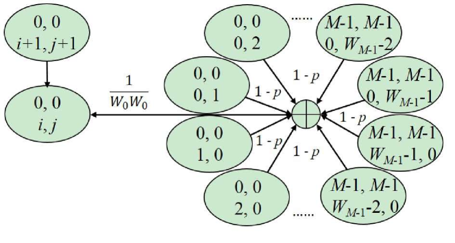
(a) State transition of cases 1, $m=n=0$.

                  

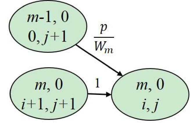
(b) State transition of case 2, $0<m<M-1,n=0$.

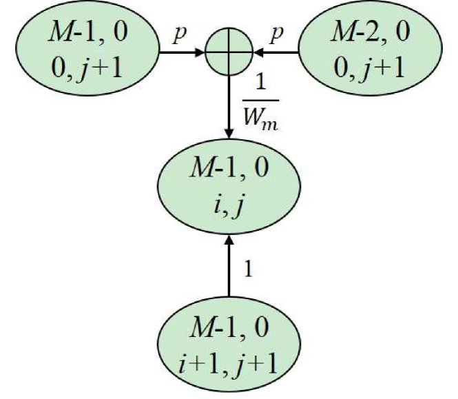
(c) State transition of case 3, $m=M-1,n=0$.

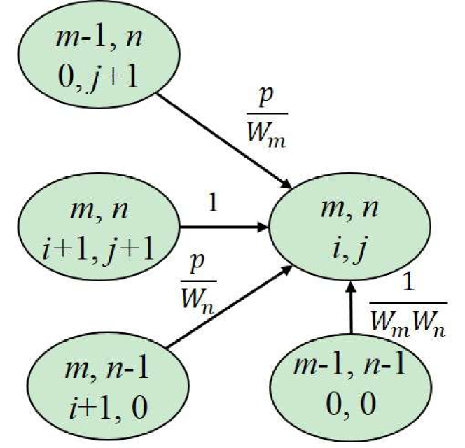
(d) State transition of case 4, $0\leq m,n\leq M-1$.

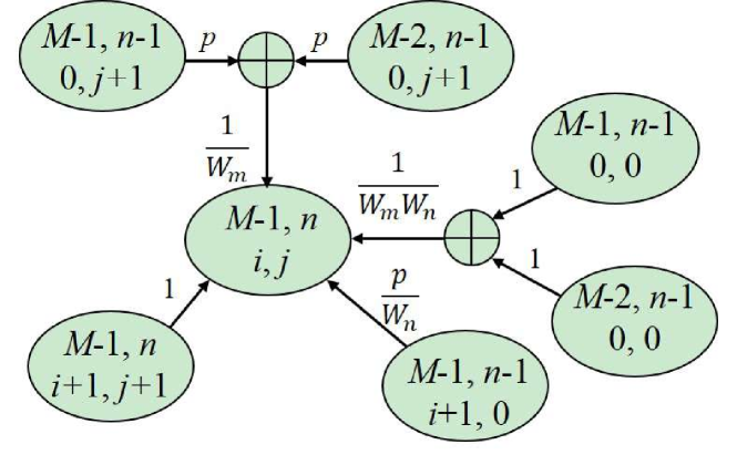
(e) State transition of case 5, $0<m<M-1,n=M-1$.

                              

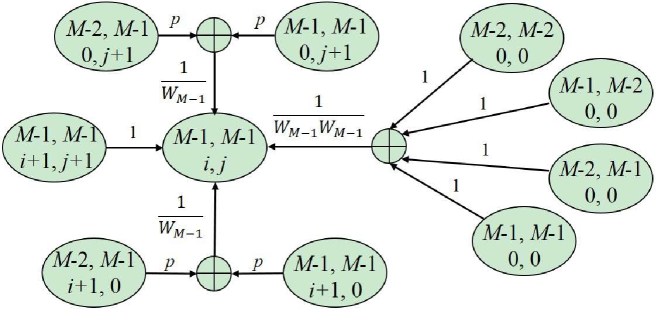
(f) State transition of case 6, $m=n=M-1$.

Figure 4: State transition of the cases 1-6.

Finally, we summarize the state probabilities and related state transition of the $7$ cases in the second and third columns of Table IV, and the proof is detailed in Appendix A.

IV Collision Probability and Throughput Analysis

IV-A Numerical Solution of Collision Probability

For the collision probability in Equation (3), we adopt Newton method to obtain its numerical solution of $\hat{p}$ since the relationship between $p$ and $\eta$ is highly nonlinear. After direct calculation, we have the iteration process given by

$$\hat{p}^{(v+1)}=\hat{p}^{(v)}-\bigg{[}\Big{(}1-\eta|_{p=\hat{p}^{(v)}}\Big{)}^{N-1}+\hat{p}^{(v)}-1\bigg{]}\bigg{[}\Big{(}N-1\Big{)}\Big{(}1-\eta|_{p=\hat{p}^{(v)}}\Big{)}^{N-2}\frac{\partial\eta}{\partial p}\bigg{|}_{p=\hat{p}^{(v)}}\bigg{]}^{-1},$$ (19)

where $\hat{p}^{(v)}$, $\eta|_{p=\hat{p}^{(v)}}$ and $\frac{\partial\eta}{\partial p}\bigg{|}_{p=\hat{p}^{(v)}}$ are the numerical values of $p$, $\eta$ and $\frac{\partial\eta}{\partial p}$ in the $v$-th iteration, respectively; and the initial $\hat{p}^{(0)}$ should take value in range $(0,1)$. For Equation (19), we give a method to calculate $\eta$ and $\frac{\partial\eta}{\partial p}$ based on the state transition model.

According to Equation (4), $\eta$ depends on the state probabilities with either $i=0$ or $j=0$. Let $\epsilon_{m,n}=\mathbb{P}(m,n,0,0),\boldsymbol{\mathrm{r}}_{m,n}=[\mathbb{P}(m,n,0,1),\mathbb{P}(m,n,0,2),\cdots,\mathbb{P}(m,n,0,W_{n}-1)]^{T}$ and $\boldsymbol{\mathrm{d}}_{m,n}=[\mathbb{P}(m,n,1,0),\mathbb{P}(m,n,2,0),\cdots,\mathbb{P}(m,n,W_{m}-1,0)]^{T}$ for $0\leq m,n\leq M-1$. The state probabilities in Equations (12)-(18) can be expressed in vector form in Theorem 1 based on the transition matrices $\boldsymbol{\mathrm{A}}_{r,r,m,n},\boldsymbol{\mathrm{A}}_{d,r,m,n},\boldsymbol{\mathrm{A}}_{r,d,m,n}$ and $\boldsymbol{\mathrm{A}}_{d,d,m,n}$ given in Figures 5(a)$-$5(d), respectively.

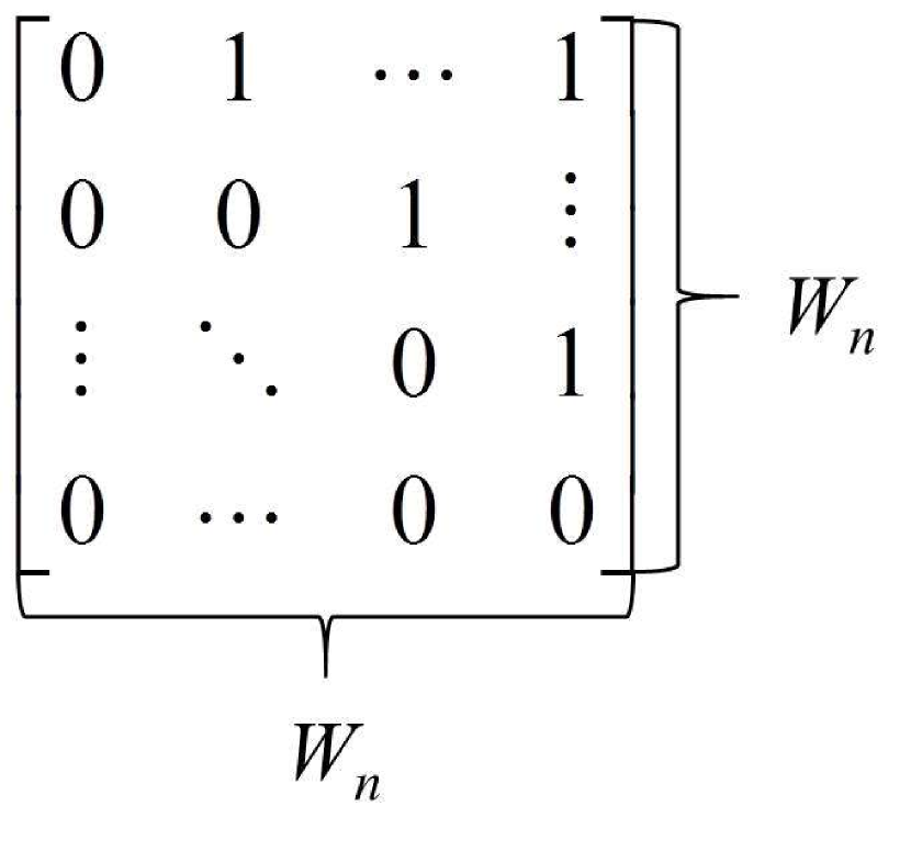
(a) $\boldsymbol{\mathrm{A}}_{r,r,m,n}$.

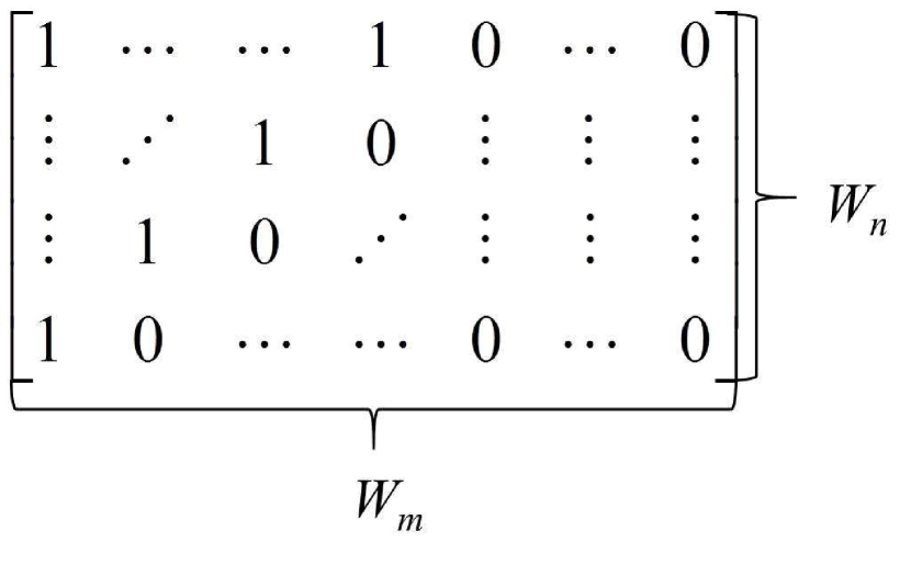
(b) $\boldsymbol{\mathrm{A}}_{d,r,m,n}$.

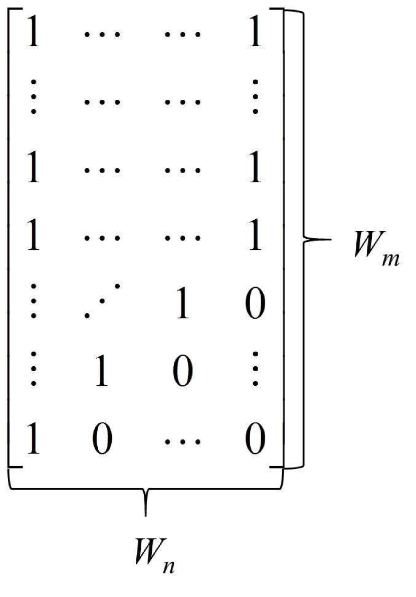
(c) $\boldsymbol{\mathrm{A}}_{r,d,m,n}$.

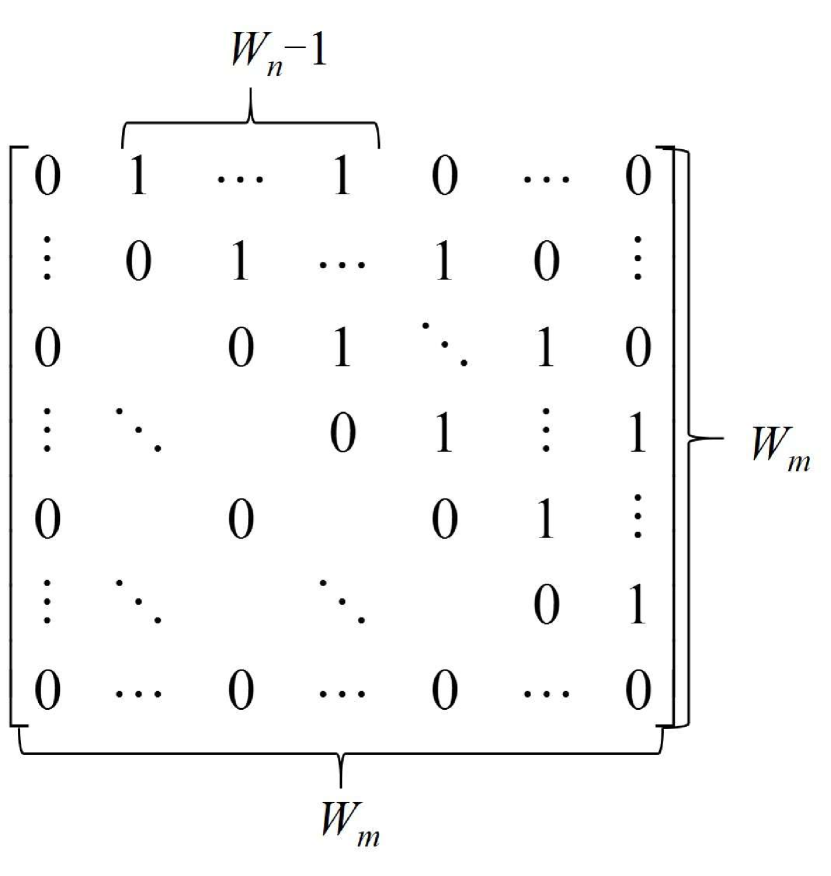
(d) $\boldsymbol{\mathrm{A}}_{d,d,m,n}$.

Figure 5: The transition matrices.

Theorem 1.

The vector form of state probabilities corresponding to the $7$ cases in Equations (12)-(18) can be summarized as follows,

Case 1: For $m=0,n=0$ and $0\leq i,j\leq W_{0}-1$, we have

$$r_{0,0,i}=d_{0,0,i}=(W_{0}-i)W_{0}^{-1}\epsilon_{0,0}.$$ (20)

Case 2: For $0<m<M-1$ and $n=0$, we have

$$\boldsymbol{\mathrm{r}}_{m,0} =W_{m}^{-1}p\boldsymbol{\mathrm{A}}_{r,r,m,n}\boldsymbol{\mathrm{r}}_{m-1,0},$$ (21)

$$\boldsymbol{\mathrm{d}}_{m,0} =W_{m}^{-1}p\boldsymbol{\mathrm{A}}_{r,d,m,n}\boldsymbol{\mathrm{r}}_{m-1,0},$$

$$\epsilon_{m,0} =W_{m}^{-1}p\boldsymbol{1}^{T}_{W_{n}-1}\boldsymbol{\mathrm{r}}_{m-1,0}.$$

Case 3: For $n=0$ and $m=M-1$, we have

$$\boldsymbol{\mathrm{r}}_{M-1,0} =(\boldsymbol{I}-W_{M-1}^{-1}p\boldsymbol{\mathrm{A}}_{r,r,m,n})^{-1}(W_{M-1}^{-1}p\boldsymbol{\mathrm{A}}_{r,r,m,n}\boldsymbol{\mathrm{r}}_{M-2,0}),$$ (22)

$$\boldsymbol{\mathrm{d}}_{M-1,0} =W_{M-1}^{-1}p\boldsymbol{\mathrm{A}}_{r,d,m,n}(\boldsymbol{\mathrm{r}}_{M-2,0}+\boldsymbol{\mathrm{r}}_{M-1,0}),$$

$$\epsilon_{M-1,0} =W_{M-1}^{-1}p\boldsymbol{1}^{T}_{W_{n}-1}(\boldsymbol{\mathrm{r}}_{M-2,0}+\boldsymbol{\mathrm{r}}_{M-1,0}).$$

Case 4: For $0<n\leq m<M-1$, we have

$$\boldsymbol{\mathrm{r}}_{m,n} =W_{m}^{-1}p\boldsymbol{\mathrm{A}}_{r,r,m,n}\boldsymbol{\mathrm{r}}_{m-1,n}+W_{n}^{-1}p\boldsymbol{\mathrm{A}}_{d,r,m,n}\boldsymbol{\mathrm{d}}_{m,n-1}+W_{m}^{-1}W_{n}^{-1}\epsilon_{m-1,n-1}\boldsymbol{\mathrm{u}}_{n,n},$$ (23)

$$\boldsymbol{\mathrm{d}}_{m,n} =W_{m}^{-1}p\boldsymbol{\mathrm{A}}_{r,d,m,n}\boldsymbol{\mathrm{r}}_{m-1,0}+W_{n}^{-1}p\boldsymbol{\mathrm{A}}_{d,d,m,n}\boldsymbol{\mathrm{d}}_{m,n-1}+W_{m}^{-1}W_{n}^{-1}\epsilon_{m-1,n-1}\boldsymbol{\mathrm{u}}_{m,n},$$

$$\epsilon_{m,n} =W_{m}^{-1}p\boldsymbol{1}^{T}_{W_{n}-1}\boldsymbol{\mathrm{r}}_{m-1,n}+W_{n}^{-1}p\boldsymbol{1}^{T}_{W_{n}}\boldsymbol{\mathrm{d}}_{m,n-1,[1,W_{n}]}+W_{m}^{-1}\epsilon_{m-1,n-1},$$

where $\boldsymbol{u}_{m,n}=\underbrace{[W_{n},W_{n},\cdots,W_{n},W_{n}-1,\cdots,1]}_{W_{m}}$.

Case 5: For $m=M-1$ and $0<n<M-1$, we have

$$\boldsymbol{\mathrm{r}}_{M-1,n} =\!(\boldsymbol{I}\!\!-\!\!W_{M-1}^{-1}\!p\boldsymbol{\mathrm{A}}_{r,r,m,n})^{-1}\!\big{[}W_{M-1}^{-1}\!p\boldsymbol{\mathrm{A}}_{r,r,m,n}\boldsymbol{\mathrm{r}}_{M-2,n}\!\!+\!\!W_{n}^{-1}\!p\boldsymbol{\mathrm{A}}_{d,r,m,n}\boldsymbol{\mathrm{d}}_{M-1,n-1}\!\!+\!\!W_{M-1}^{-1}\!\!W_{n}^{-1}\!(\!\epsilon_{M-2,n-1}\!\!+\!\epsilon_{M-1,n-1}\!)\boldsymbol{\mathrm{u}}_{n,n}\big{]},$$ (24)

$$\boldsymbol{\mathrm{d}}_{M-1,n} =W_{M-1}^{-1}p\boldsymbol{\mathrm{A}}_{r,d,m,n}(\boldsymbol{\mathrm{r}}_{M-2,n}\!+\!\boldsymbol{\mathrm{r}}_{M-1,n})\!+\!W_{n}^{-1}p\boldsymbol{\mathrm{A}}_{d,d,m,n}\boldsymbol{\mathrm{d}}_{M-1,n-1}\!+\!W_{M-1}^{-1}W_{n}^{-1}(\epsilon_{M-2,n-1}\!+\!\epsilon_{M-1,n-1})\boldsymbol{\mathrm{u}}_{M-1,n},$$

$$\epsilon_{M-1,n} =W_{M-1}^{-1}p\boldsymbol{1}^{T}_{W_{n}-1}(\boldsymbol{\mathrm{r}}_{M-2,n}+\boldsymbol{\mathrm{r}}_{M-1,n})+W_{n}^{-1}p\boldsymbol{1}^{T}_{W_{n}}\boldsymbol{\mathrm{d}}_{M-1,n-1,[1,W_{n}]}+W_{M-1}^{-1}(\epsilon_{M-2,n-1}+\epsilon_{M-1,n-1}).$$

Case 6: For $m=n=M-1$, we have

$$\epsilon_{M-1,M-1} =\Big{[}1-2W_{M-1}^{-3}p\boldsymbol{1}^{T}_{W_{M-1}-1}\big{(}\boldsymbol{I}-W_{M-1}^{-1}p\boldsymbol{A}^{\sigma}\big{)}^{-1}\boldsymbol{u}_{M-1,M-1}-W_{M-1}^{-1}\Big{]}^{-1}\Big{[}2W_{M-1}^{-1}p\boldsymbol{1}^{T}_{W_{M-1}-1}\boldsymbol{\mathrm{d}}_{M-1,M-2}$$ (25)

$$+W_{M-1}^{-1}\epsilon^{\sigma}+2W_{M-1}^{-1}p\boldsymbol{1}^{T}_{W_{M-1}-1}\big{(}\boldsymbol{I}-W_{M-1}^{-1}p\boldsymbol{A}^{\sigma}\big{)}^{-1}\big{(}W_{M-1}^{-1}p\boldsymbol{A}^{\sigma}\boldsymbol{\mathrm{d}}_{M-1,M-2}+W_{M-1}^{-2}\epsilon^{\sigma}\boldsymbol{u}_{M-1,M-1}\big{)}\Big{]},$$

$$\boldsymbol{\mathrm{r}}_{M-1,M-1} =\boldsymbol{\mathrm{d}}_{M-1,M-1}$$

$$=\big{(}\boldsymbol{I}-W_{M-1}^{-1}p\boldsymbol{A}^{\sigma}\big{)}^{-1}\big{[}W_{M-1}^{-1}p\boldsymbol{A}^{\sigma}\boldsymbol{\mathrm{d}}_{M-1,M-2}+W_{M-1}^{-2}(\epsilon^{\sigma}+\epsilon_{M-1,M-1})\boldsymbol{u}_{M-1,M-1}\big{]},$$

where $\boldsymbol{A}^{\sigma}=\boldsymbol{A}_{r,r,M-1,M-1}+\boldsymbol{A}_{r,d,M-1,M-1}=\boldsymbol{A}_{d,d,M-1,M-1}+\boldsymbol{A}_{d,r,M-1,M-1}$ and $\epsilon^{\sigma}=\epsilon_{M-2,M-2}+\epsilon_{M-2,M-1}+\epsilon_{M-1,M-2}$.

Case 7: For $0\leq m<n\leq M-1$, we have $\boldsymbol{\mathrm{r}}_{m,n}=\boldsymbol{\mathrm{d}}_{n,m},\boldsymbol{\mathrm{d}}_{m,n}=\boldsymbol{\mathrm{r}}_{n,m},\epsilon_{m,n}=\epsilon_{n,m}$.

Proof: Please refer to Appendix B.

Based on Theorem 1, we can use $\epsilon_{0,0}$ to obtain $r_{m,n,i},d_{m,n,j}$ and $\epsilon_{m,n}$ for $0\leq m,n\leq M-1$, where $r_{m,n,i}$ and $d_{m,n,j}$ are the $i$-th and $j$-th element of $\boldsymbol{\mathrm{r}}_{m,n}$ and $\boldsymbol{\mathrm{d}}_{m,n}$, respectively, for $0\leq i\leq W_{m}-1,0\leq j\leq W_{n}-1$. Since $\sum_{m=0}^{M-1}\sum_{n=0}^{M-1}\sum_{i=0}^{W_{m}-1}\sum_{j=0}^{W_{n}-1}\mathbb{P}(m,n,i,j)=1$, letting $\mathbb{P}(m,n)=\sum_{i=0}^{W_{m}-1}\sum_{j=0}^{W_{n}-1}\mathbb{P}(m,n,i,j)$ denote the probability that the contention windows of $T_{1}$ and $T_{2}$ equal $W_{m}$ and $W_{n}$, respectively, we have the following Theorem 2 to calculate $\mathbb{P}(m,n)$ for $0\leq m,n\leq M-1$.

Theorem 2.

Corresponding to the $7$ cases in Theorem 1, probability $\mathbb{P}(m,n)$ can be calculated as follows,

Case 1: For $m=n=0$, we have

$$\mathbb{P}(0,0)=\frac{1}{6}(2W_{0}+1)(W_{0}+1)\epsilon_{0,0}.$$ (26)

Case 2: For $0<m<M-1$ and $n=0$, we have

$$\mathbb{P}(m,0)=W_{m}^{-1}p\sum^{W_{0}-1}_{i=1}r_{m-1,0,i}\bigg{[}-\frac{1}{2}i^{2}+\Big{(}W_{m}+\frac{1}{2}\Big{)}i\bigg{]}.$$ (27)

Case 3: For $m=M-1$ and $n=0$, we have

$$\mathbb{P}(M-1,0)=W_{M-1}^{-1}p\sum^{W_{0}-1}_{i=1}(r_{M-2,0,i}+r_{M-1,0,i})\bigg{[}-\frac{1}{2}i^{2}+\Big{(}W_{M-1}+\frac{1}{2}\Big{)}i\bigg{]}.$$ (28)

Case 4: For $0<n\leq m<M-1$, we have

$$\mathbb{P}(m,n) =W_{m}^{-1}p\sum^{W_{n}-1}_{i=1}r_{m-1,n,i}\bigg{[}-\frac{1}{2}i^{2}+\Big{(}W_{m}+\frac{1}{2}\Big{)}i\bigg{]}+W_{n}^{-1}p\sum^{W_{n}-1}_{i=1}d_{m,n-1,i}\bigg{[}-\frac{1}{2}i^{2}+\Big{(}W_{n}+\frac{1}{2}\Big{)}i\bigg{]}$$ (29)

$$+\!W_{n}^{-1}\!p\!\!\sum^{W_{m}-1}_{i=W_{n}}\!\!d_{m,n-1,i}\Big{(}\!-\!\frac{1}{2}W_{n}^{2}\!+\!\frac{1}{2}W_{n}\Big{)}\!+\!W_{m}^{-1}W_{n}^{-1}\epsilon_{m-1,n-1}\Big{(}\!-\!\frac{1}{6}W_{n}^{3}\!+\!\frac{1}{2}W_{m}W_{n}^{2}\!+\!\frac{1}{2}W_{m}W_{n}\!+\!\frac{1}{6}W_{n}\Big{)}.$$

Case 5: For $m=M-1$ and $0<n<M-1$, we have

$$\mathbb{P}(M-1,n) =W_{M-1}^{-1}p\!\!\!\!\sum^{W_{n}-1}_{i=1}\!\!(r_{M-2,n,i}\!+\!r_{M-1,n,i})\bigg{[}-\frac{1}{2}i^{2}\!+\!\Big{(}W_{M-1}\!+\!\frac{1}{2}\Big{)}i\bigg{]}\!+\!W_{n}^{-1}p\!\!\!\!\sum^{W_{n}-1}_{i=1}\!\!\!\!d_{M-1,n-1,i}\bigg{[}-\frac{1}{2}i^{2}\!+\!\Big{(}W_{n}\!+\!\frac{1}{2}\Big{)}i\bigg{]}$$ (30)

$$+\!\!W_{n}^{-1}p\!\!\!\!\!\sum^{W_{M-1}-1}_{i=W_{n}}\!\!\!\!\!d_{M-1,n-1,i}\Big{(}-\!\!\frac{1}{2}W_{n}^{2}\!+\!\frac{1}{2}W_{n}\Big{)}\!+\!W_{M-1}^{-1}W_{n}^{-1}\epsilon^{\sigma}\Big{(}-\!\!\frac{1}{6}W_{n}^{3}\!\!+\!\!\frac{1}{2}W_{M-1}W_{n}^{2}\!\!+\!\!\frac{1}{2}W_{M-1}W_{n}\!\!+\!\!\frac{1}{6}W_{n}\Big{)},$$

where $\epsilon^{\sigma}=\epsilon_{M-2,n-1}+\epsilon_{M-1,n-1}$.

Case 6: For $m=M-1$ and $n=M-1$, we have

$$\mathbb{P}(M-1,M-1) =W_{M-1}^{-1}p\sum^{W-1}_{i=1}d^{\sigma}_{i}\bigg{[}-\frac{1}{2}i^{2}+\Big{(}W_{M-1}+\frac{1}{2}\Big{)}i\bigg{]}+W_{M-1}^{-2}\epsilon^{\sigma}\Big{(}\frac{1}{3}W_{M-1}^{3}+\frac{1}{2}W_{M-1}^{2}+\frac{1}{6}W_{M-1}\Big{)},$$ (31)

where $d^{\sigma}_{i}=r_{m-1,n,i}+r_{m,n,i}+d_{m,n-1,i}+d_{m,n,i}$ and $\epsilon^{\sigma}=\epsilon_{M-2,M-2}+\epsilon_{M-2,M-1}+\epsilon_{M-1,M-2}+\epsilon_{M-1,M-1}$.

Case 7: For $0\leq m<n\leq M-1$, we have that $\mathbb{P}(m,n)=\mathbb{P}(n,m)$.

Proof: Please refer to Appendix C.

Based on Theorems 1 and 2, we can utilize $\epsilon_{0,0}$ to obtain $\mathbb{P}(m,n)$ for $0\leq m,n\leq M-1$, and adopt the condition that $\sum_{m=0}^{M-1}\sum_{n=0}^{M-1}\mathbb{P}(m,n)=1$ to calculate $\epsilon_{0,0}$. Furtherly, we adopt Theorem 1 to obtain $r_{m,n,i},d_{m,n,j}$ and $\epsilon_{m,n}$ for $0\leq i\leq W_{m}-1,0\leq j\leq W_{n}-1,0\leq m,n\leq M-1$ based on $\epsilon_{0,0}$, and calculate $\eta|_{p=\hat{p}^{(v)}}$ according to Equation (4) or its equivalent vector as follows,

$$\eta=\sum^{M-1}_{m=0}\sum^{M-1}_{n=0}\boldsymbol{1}^{T}_{W_{n}-1}\boldsymbol{\mathrm{r}}_{m,n}+\boldsymbol{1}^{T}_{W_{m}-1}\boldsymbol{\mathrm{d}}_{m,n}.$$ (32)

Moreover, in order to calculate $\frac{\partial\eta}{\partial p}|_{p=\hat{p}^{(v)}}$ in Equation (19), we have that

$$\frac{\partial\eta}{\partial p}=\sum_{m=0}^{M-1}\sum_{n=0}^{M-1}\boldsymbol{1}^{T}_{W_{n}-1}\nabla_{p}\boldsymbol{\mathrm{r}}_{m,n}+\boldsymbol{1}^{T}_{W_{m}-1}\nabla_{p}\boldsymbol{\mathrm{d}}_{m,n},$$ (33)

where $\nabla_{p}\boldsymbol{\mathrm{r}}_{m,n}=\Big{[}\frac{\partial\mathbb{P}(m,n,0,1)}{\partial p},\frac{\partial\mathbb{P}(m,n,0,2)}{\partial p},\cdots,\frac{\partial\mathbb{P}(m,n,0,\mathbb{P}(m,n,0,W_{n}-1))}{\partial p}\Big{]}^{T}$ and $\nabla_{p}\boldsymbol{\mathrm{d}}_{m,n}=\Big{[}\frac{\partial\mathbb{P}(m,n,1,0)}{\partial p},\frac{\partial\mathbb{P}(m,n,2,0)}{\partial p},\\ \cdots,\frac{\partial\mathbb{P}(m,n,W_{m}-1,0)}{\partial p}\Big{]}^{T}$. According to Theorem 1, we have Lemma 1 to calculate $\nabla_{p}\boldsymbol{\mathrm{r}}_{m,n},\nabla_{p}\boldsymbol{\mathrm{d}}_{m,n}$ and $\frac{\partial\epsilon_{m,n}}{\partial p}$ as follows, where the proof is omitted since it is based on standard calculus.

Lemma 1.

Corresponding to the $7$ cases in Theorem 1, $\nabla_{p}\boldsymbol{\mathrm{r}}_{m,n},\nabla_{p}\boldsymbol{\mathrm{d}}_{m,n}$ and $\frac{\partial\epsilon_{m,n}}{\partial p}$ can be characterized as follows,

Case 1: For $m=n=0$, and $0\leq i,j\leq W_{0}-1$, we have

$$\frac{\partial r_{0,0,i}}{\partial p}=\frac{\partial d_{0,0,i}}{\partial p}=(W_{0}-i)W_{0}^{-1}\frac{\partial\epsilon_{0,0}}{\partial p}.$$ (34)

Case 2: For $0<m<M-1$ and $n=0$, we have

$$\nabla_{p}\boldsymbol{\mathrm{r}}_{m,0} =W_{m}^{-1}\boldsymbol{\mathrm{A}}_{r,r,m,n}(\nabla_{p}\boldsymbol{\mathrm{r}}_{m-1,0}+p\nabla_{p}\boldsymbol{\mathrm{r}}_{m-1,0}),$$ (35)

$$\nabla_{p}\boldsymbol{\mathrm{d}}_{m,0} =W_{m}^{-1}\boldsymbol{\mathrm{A}}_{r,d,m,n}(\nabla_{p}\boldsymbol{\mathrm{r}}_{m-1,0}+p\nabla_{p}\boldsymbol{\mathrm{r}}_{m-1,0}),$$

$$\frac{\partial\epsilon_{m,0}}{\partial p} =W_{m}^{-1}\boldsymbol{1}^{T}_{W_{n}-1}(\nabla_{p}\boldsymbol{\mathrm{r}}_{m-1,0}+p\nabla_{p}\boldsymbol{\mathrm{r}}_{m-1,0}).$$

Case 3: For $m=M-1$ and $n=0$, we have

$$\nabla_{p}\boldsymbol{\mathrm{r}}_{M-1,0} =(\boldsymbol{I}-W_{M-1}^{-1}p\boldsymbol{\mathrm{A}}_{r,r,m,n})^{-1}W_{M-1}^{-1}p\boldsymbol{\mathrm{A}}_{r,r,m,n}(\nabla_{p}\boldsymbol{\mathrm{r}}_{M-2,0}+\nabla_{p}\boldsymbol{\mathrm{r}}_{M-1,0}+p\nabla_{p}\boldsymbol{\mathrm{r}}_{M-2,0}),$$ (36)

$$\nabla_{p}\boldsymbol{\mathrm{d}}_{M-1,0} =W_{M-1}^{-1}\boldsymbol{\mathrm{A}}_{r,d,m,n}(\nabla_{p}\boldsymbol{\mathrm{r}}_{M-2,0}+\nabla_{p}\boldsymbol{\mathrm{r}}_{M-1,0}+p\nabla_{p}\boldsymbol{\mathrm{r}}_{M-2,0}+p\nabla_{p}\boldsymbol{\mathrm{r}}_{M-1,0}),$$

$$\frac{\partial\epsilon_{M-1,0}}{\partial p} =W_{M-1}^{-1}\boldsymbol{1}^{T}_{W_{n}-1}(\nabla_{p}\boldsymbol{\mathrm{r}}_{M-2,0}+\nabla_{p}\boldsymbol{\mathrm{r}}_{M-1,0}+p\nabla_{p}\boldsymbol{\mathrm{r}}_{M-2,0}+p\nabla_{p}\boldsymbol{\mathrm{r}}_{M-1,0}).$$

Case 4: For $0<n\leq m<M-1$, we have

$$\nabla_{p}\boldsymbol{\mathrm{r}}_{m,n} =W_{m}^{-1}\boldsymbol{\mathrm{A}}_{r,r,m,n}(\nabla_{p}\boldsymbol{\mathrm{r}}_{m-1,n}\!\!+\!\!p\nabla_{p}\boldsymbol{\mathrm{r}}_{m-1,n})\!\!+\!\!W_{n}^{-1}\boldsymbol{\mathrm{A}}_{d,r,m,n}(\nabla_{p}\boldsymbol{\mathrm{d}}_{m,n-1}\!\!+\!\!p\nabla_{p}\boldsymbol{\mathrm{d}}_{m,n-1})\!\!+\!\!W_{m}^{-1}W_{n}^{-1}\frac{\partial\epsilon_{m-1,n-1}}{\partial p}\boldsymbol{\mathrm{u}}_{n,n},$$ (37)

$$\nabla_{p}\boldsymbol{\mathrm{d}}_{m,n} =W_{m}^{-1}\boldsymbol{\mathrm{A}}_{r,d,m,n}(\nabla_{p}\boldsymbol{\mathrm{r}}_{m-1,n}\!\!+\!\!p\nabla_{p}\boldsymbol{\mathrm{r}}_{m-1,n})\!\!+\!\!W_{n}^{-1}\boldsymbol{\mathrm{A}}_{d,d,m,n}(\nabla_{p}\boldsymbol{\mathrm{d}}_{m,n-1}\!\!+\!\!p\nabla_{p}\boldsymbol{\mathrm{d}}_{m,n-1})\!\!+\!\!W_{m}^{-1}W_{n}^{-1}\frac{\partial\epsilon_{m-1,n-1}}{\partial p}\boldsymbol{\mathrm{u}}_{m,n},$$

$$\frac{\partial\epsilon_{m,n}}{\partial p} =W_{m}^{-1}\boldsymbol{1}^{T}_{W_{n}-1}(\nabla_{p}\boldsymbol{\mathrm{r}}_{m-1,n}\!+\!p\nabla_{p}\boldsymbol{\mathrm{r}}_{m-1,n})\!+\!W_{n}^{-1}\boldsymbol{1}^{T}_{W_{n}}(\nabla_{p}\boldsymbol{\mathrm{d}}_{m,n-1,[1,W_{n}]}\!+\!p\nabla_{p}\boldsymbol{\mathrm{d}}_{m,n-1,[1,W_{n}]})\!+\!W_{m}^{-1}\frac{\partial\epsilon_{m-1,n-1}}{\partial p}.$$

Case 5: For $m=M-1$ and $0<n<M-1$, we have

$$\nabla_{p}\boldsymbol{\mathrm{r}}_{M-1,n} =(\boldsymbol{I}-W_{M-1}^{-1}p\boldsymbol{\mathrm{A}}_{r,r,m,n})^{-1}\bigg{[}W_{M-1}^{-1}\boldsymbol{\mathrm{A}}_{r,r,m,n}(\nabla_{p}\boldsymbol{\mathrm{r}}_{M-2,n}+\nabla_{p}\boldsymbol{\mathrm{r}}_{M-1,n}+p\nabla_{p}\boldsymbol{\mathrm{r}}_{M-2,n})+W_{n}^{-1}\boldsymbol{\mathrm{A}}_{d,r,m,n}$$ (38)

$$(\nabla_{p}\boldsymbol{\mathrm{d}}_{M-1,n-1}+p\nabla_{p}\boldsymbol{\mathrm{d}}_{M-1,n-1})+W_{M-1}^{-1}W_{n}^{-1}\Big{(}\frac{\partial\epsilon_{M-2,n-1}}{\partial p}+\frac{\partial\epsilon_{M-1,n-1}}{\partial p}\Big{)}\boldsymbol{\mathrm{u}}_{n,n}\bigg{]},$$

$$\nabla_{p}\boldsymbol{\mathrm{d}}_{M-1,n} =W_{M-1}^{-1}\boldsymbol{\mathrm{A}}_{r,d,m,n}(\nabla_{p}\boldsymbol{\mathrm{r}}_{M-2,n}+\nabla_{p}\boldsymbol{\mathrm{r}}_{M-1,n}+p\nabla_{p}\boldsymbol{\mathrm{r}}_{M-2,n}+p\nabla_{p}\boldsymbol{\mathrm{r}}_{M-1,n})+W_{n}^{-1}p\boldsymbol{\mathrm{A}}_{d,d,m,n}(\nabla_{p}\boldsymbol{\mathrm{d}}_{M-1,n-1}+$$

$$p\nabla_{p}\boldsymbol{\mathrm{d}}_{M-1,n-1})+W_{M-1}^{-1}W_{n}^{-1}\Big{(}\frac{\partial\epsilon_{M-2,n-1}}{\partial p}+\frac{\partial\epsilon_{M-1,n-1}}{\partial p}\Big{)}\boldsymbol{\mathrm{u}}_{M-1,n},$$

$$\frac{\partial\epsilon_{M-1,n}}{\partial p} =W_{M-1}^{-1}\boldsymbol{1}^{T}_{W_{n}-1}(\nabla_{p}\boldsymbol{\mathrm{r}}_{M-2,n}+\nabla_{p}\boldsymbol{\mathrm{r}}_{M-1,n}+p\nabla_{p}\boldsymbol{\mathrm{r}}_{M-2,n}+p\nabla_{p}\boldsymbol{\mathrm{r}}_{M-1,n})+W_{n}^{-1}\boldsymbol{1}^{T}_{W_{n}}(\nabla_{p}\boldsymbol{\mathrm{d}}_{M-1,n-1,[1,W_{n}]}+$$

$$p\nabla_{p}\boldsymbol{\mathrm{d}}_{M-1,n-1,[1,W_{n}]})+W_{M-1}^{-1}\Big{(}\frac{\partial\epsilon_{M-2,n-1}}{\partial p}+\frac{\partial\epsilon_{M-1,n-1}}{\partial p}\Big{)}.$$

Case 6: For $m=n=M-1$, we have

$$\frac{\partial\epsilon_{M-1,M-1}}{\partial p} =\Big{[}1-2W_{M-1}^{-3}p\boldsymbol{1}^{T}_{W_{M-1}-1}\big{(}\boldsymbol{I}-W_{M-1}^{-1}p\boldsymbol{A}^{\sigma}\big{)}^{-1}\boldsymbol{u}_{M-1,M-1}-W_{M-1}^{-1}\Big{]}^{-1}\bigg{\{}2W_{M-1}^{-1}\boldsymbol{1}^{T}_{W_{M-1}-1}(\nabla_{p}\boldsymbol{\mathrm{d}}_{M-1,M-2}+$$ (39)

$$\nabla_{p}\boldsymbol{\mathrm{d}}_{M-1,M-1}+p\nabla_{p}\boldsymbol{\mathrm{d}}_{M-1,M-2})+W_{M-1}^{-1}\frac{\partial\epsilon^{\sigma}}{\partial p}+2W_{M-1}^{-1}p\boldsymbol{1}^{T}_{W_{M-1}-1}\big{(}\boldsymbol{I}-W_{M-1}^{-1}p\boldsymbol{A}^{\sigma}\big{)}^{-1}\Big{[}W_{M-1}^{-1}\boldsymbol{A}^{\sigma}$$

$$(\nabla_{p}\boldsymbol{\mathrm{d}}_{M-1,M-2}+\nabla_{p}\boldsymbol{\mathrm{d}}_{M-1,M-1}+p\nabla_{p}\boldsymbol{\mathrm{d}}_{M-1,M-2})+W_{M-1}^{-2}\frac{\partial\epsilon^{\sigma}}{\partial p}\boldsymbol{u}_{M-1,M-1}\Big{]}\bigg{\}},$$

$$\nabla_{p}\boldsymbol{\mathrm{r}}_{M-1,M-1} =\nabla_{p}\boldsymbol{\mathrm{d}}_{M-1,M-1}$$

$$=\big{(}\boldsymbol{I}-W_{M-1}^{-1}p\boldsymbol{A}^{\sigma}\big{)}^{-1}\bigg{[}W_{M-1}^{-1}p\boldsymbol{A}^{\sigma}(\nabla_{p}\boldsymbol{\mathrm{d}}_{M-1,M-2}+\nabla_{p}\boldsymbol{\mathrm{d}}_{M-1,M-1}+p\nabla_{p}\boldsymbol{\mathrm{d}}_{M-1,M-2})$$

$$+W_{M-1}^{-2}\Big{(}\frac{\partial\epsilon^{\sigma}}{\partial p}+\frac{\partial\epsilon_{M-1,M-1}}{\partial p}\Big{)}\boldsymbol{u}_{M-1,M-1}\bigg{]},$$

where $\boldsymbol{A}^{\sigma}=\boldsymbol{A}_{r,r,M-1,M-1}+\boldsymbol{A}_{r,d,M-1,M-1}=\boldsymbol{A}_{d,d,M-1,M-1}+\boldsymbol{A}_{d,r,M-1,M-1}$; and

$$\frac{\partial\epsilon^{\sigma}}{\partial p}=\frac{\partial\epsilon_{M-2,M-2}}{\partial p}+\frac{\partial\epsilon_{M-2,M-1}}{\partial p}+\frac{\partial\epsilon_{M-1,M-2}}{\partial p}.$$ (40)

Case 7: For $0\leq m<n\leq M-1$, we have that $\nabla_{p}\boldsymbol{\mathrm{r}}_{m,n}=\nabla_{p}\boldsymbol{\mathrm{d}}_{n,m},\nabla_{p}\boldsymbol{\mathrm{d}}_{m,n}=\nabla_{p}\boldsymbol{\mathrm{r}}_{n,m},\frac{\partial\epsilon_{m,n}}{\partial p}=\frac{\partial\epsilon_{n,m}}{\partial p}$.

According to Lemma 1, we can utilize $\epsilon_{0,0}$ and $\frac{\partial\epsilon_{0,0}}{\partial p}$ to obtain $\nabla_{p}\boldsymbol{\mathrm{r}}_{m,n},\nabla_{p}\boldsymbol{\mathrm{d}}_{m,n}$ and $\frac{\partial\epsilon_{m,n}}{\partial p}$ for $0\leq m,n\leq M-1$. Furthermore, the normalization condition of $\nabla_{p}\boldsymbol{\mathrm{r}}_{m,n},\nabla_{p}\boldsymbol{\mathrm{d}}_{m,n}$ and $\frac{\partial\epsilon_{m,n}}{\partial p}$ is given by the following equation,

$$\sum_{m=0}^{M-1}\sum_{n=0}^{M-1}\frac{\partial\mathbb{P}(m,n)}{\partial p}=\frac{\partial}{\partial p}\sum_{m=0}^{M-1}\sum_{n=0}^{M-1}\mathbb{P}(m,n)=0.$$ (41)

Therefore, we propose the following Lemma 2 to calculate $\frac{\partial\mathbb{P}(m,n)}{\partial p}$ using $\nabla_{p}\boldsymbol{\mathrm{r}}_{m,n},\nabla_{p}\boldsymbol{\mathrm{d}}_{m,n}$ and $\frac{\partial\epsilon_{m,n}}{\partial p}$ for $0\leq m,n\leq M-1$.

Lemma 2.

Based on the $7$ cases in Theorem 2, the partial derivative $\frac{\partial\mathbb{P}(m,n)}{\partial p}$ for $0\leq m,n\leq M-1$ can be computed as follows,

Case 1: For $m=n=0$, we have

$$\frac{\partial\mathbb{P}(0,0)}{\partial p}=\frac{1}{6}(2W_{0}+1)(W_{0}+1)\frac{\partial\epsilon_{0,0}}{\partial p}.$$ (42)

Case 2: For $0<m<M-1$, and $n=0$, we have

$$\frac{\partial\mathbb{P}(m,0)}{\partial p}=W_{m}^{-1}\sum^{W_{0}-1}_{i=1}\Big{(}k\frac{\partial}{\partial p}r_{m-1,0,i}+p\frac{\partial r_{m-1,0,i}}{\partial p}\Big{)}\bigg{[}-\frac{1}{2}i^{2}+\Big{(}W_{m}+\frac{1}{2}\Big{)}i\bigg{]}.$$ (43)

Case 3: For $m=M-1$ and $n=0$, we have

$$\frac{\partial\mathbb{P}(M-1,0)}{\partial p}=W_{M-1}^{-1}\sum^{W_{0}-1}_{i=1}\Big{(}k\frac{\partial}{\partial p}r_{M-2,0,i}\!+\!k\frac{\partial}{\partial p}r_{M-1,0,i}\!+\!p\frac{\partial r_{M-2,0,i}}{\partial p}\!+\!p\frac{\partial r_{M-1,0,i}}{\partial p}\Big{)}\bigg{[}-\frac{1}{2}i^{2}\!+\!\Big{(}W_{M-1}\!+\!\frac{1}{2}\Big{)}i\bigg{]}.$$ (44)

Case 4: For $0<n\leq m<M-1$, we have

$$\frac{\partial\mathbb{P}(m,n)}{\partial p} =W_{m}^{-1}\sum^{W_{n}-1}_{i=1}\Big{(}k\frac{\partial}{\partial p}r_{m-1,n,i}\!+\!p\frac{\partial r_{m-1,n,i}}{\partial p}\Big{)}\bigg{[}-\frac{1}{2}i^{2}\!+\!\Big{(}W_{m}+\frac{1}{2}\Big{)}i\bigg{]}\!+\!W_{n}^{-1}\sum^{W_{n}-1}_{i=1}\Big{(}k\frac{\partial}{\partial p}d_{m,n-1,i}\!+\!p\frac{\partial d_{m,n-1,i}}{\partial p}\Big{)}$$ (45)

$$\bigg{[}-\frac{1}{2}i^{2}+\Big{(}W_{n}+\frac{1}{2}\Big{)}i\bigg{]}+\Big{(}-\frac{1}{2}W_{n}+\frac{1}{2}\Big{)}\sum^{W_{m}-1}_{i=W_{n}}\Big{(}k\frac{\partial}{\partial p}d_{m,n-1,i}+p\frac{\partial d_{m,n-1,i}}{\partial p}\Big{)}+W_{m}^{-1}W_{n}^{-1}\frac{\partial\epsilon_{m-1,n-1}}{\partial p}$$

$$\Big{(}-\frac{1}{6}W_{n}^{3}+\frac{1}{2}W_{m}W_{n}^{2}+\frac{1}{2}W_{m}W_{n}+\frac{1}{6}W_{n}\Big{)}.$$

Case 5: For $m=M-1$ we have $0<n<M-1$, we have

$$\frac{\partial\mathbb{P}(M-1,n)}{\partial p}=W_{M-1}^{-1}\sum^{W_{n}-1}_{i=1}\Big{(}k\frac{\partial}{\partial p}r_{M-2,n,i}\!+\!k\frac{\partial}{\partial p}r_{M-1,n,i}\!+\!p\frac{\partial r_{M-2,n,i}}{\partial p}\!+\!p\frac{\partial r_{M-1,n,i}}{\partial p}\Big{)}\bigg{[}-\!\frac{1}{2}i^{2}\!+\!\Big{(}W_{M-1}\!+\!\frac{1}{2}\Big{)}i\bigg{]}$$ (46)

$$+W_{n}^{-1}\sum^{W_{n}-1}_{i=1}\Big{(}k\frac{\partial}{\partial p}d_{M-1,n-1,i}+p\frac{\partial d_{M-1,n-1,i}}{\partial p}\Big{)}\bigg{[}-\frac{1}{2}i^{2}+\Big{(}W_{n}+\frac{1}{2}\Big{)}i\bigg{]}+\Big{(}-\frac{1}{2}W_{n}+\frac{1}{2}\Big{)}\sum^{W_{M-1}-1}_{i=W_{n}}\Big{(}k\frac{\partial}{\partial p}d_{M-1,n-1,i}$$

$$+p\frac{\partial d_{M-1,n-1,i}}{\partial p}\Big{)}+W_{M-1}^{-1}W_{n}^{-1}\Big{(}\frac{\partial\epsilon_{M-2,n-1}}{\partial p}+\frac{\partial\epsilon_{M-1,n-1}}{\partial p}\Big{)}\Big{(}-\frac{1}{6}W_{n}^{3}+\frac{1}{2}W_{M-1}W_{n}^{2}+\frac{1}{2}W_{M-1}W_{n}+\frac{1}{6}W_{n}\Big{)}.$$

Case 6: For $m=n=M-1$, we have

$$\frac{\partial\mathbb{P}(M-1,M-1)}{\partial p} =W_{M-1}^{-1}\sum^{W-1}_{i=1}\Big{(}k\frac{\partial}{\partial p}d^{\sigma}_{i}\!+\!p\frac{\partial d^{\sigma}_{i}}{\partial p}\Big{)}\bigg{[}-\frac{1}{2}i^{2}\!+\!\Big{(}W_{M-1}\!+\!\frac{1}{2}\Big{)}i\bigg{]}\!+\!\frac{\partial\epsilon^{\sigma}}{\partial p}\Big{(}\frac{1}{3}W_{M-1}\!+\!\frac{1}{2}\!+\!\frac{1}{6}W_{M-1}^{-1}\Big{)},$$

where

$$\frac{\partial d^{\sigma}_{i}}{\partial p} =\frac{\partial r_{m-1,n,i}}{\partial p}+\frac{\partial r_{m,n,i}}{\partial p}+\frac{\partial d_{m,n-1,i}}{\partial p}+\frac{\partial d_{m,n,i}}{\partial p}$$ (47)

$$\frac{\partial\epsilon^{\sigma}}{\partial p} =\frac{\partial\epsilon_{M-2,M-2}}{\partial p}+\frac{\partial\epsilon_{M-2,M-1}}{\partial p}+\frac{\partial\epsilon_{M-1,M-2}}{\partial p}+\frac{\partial\epsilon_{M-1,M-1}}{\partial p}.$$

Case 7: For $0\leq n<m\leq M-1$, we have that $\frac{\partial\mathbb{P}(m,n)}{\partial p}=\frac{\partial\mathbb{P}(n,m)}{\partial p}$.

Based on Lemmas 1 and 2, we can use $\epsilon_{0,0}$ and $\frac{\partial\epsilon_{0,0}}{\partial p}$ to characterize $\frac{\partial\mathbb{P}(m,n)}{\partial p}$, and utilize the normalization condition give by Equation (41) to obtain $\frac{\partial\epsilon_{0,0}}{\partial p}$. Furthermore, we can calculate $\nabla_{p}\boldsymbol{\mathrm{r}}_{m,n},\nabla_{p}\boldsymbol{\mathrm{d}}_{m,n}$ and $\frac{\partial\epsilon_{m,n}}{\partial p}$ for $0\leq m,n\leq M-1$ by $\frac{\partial\epsilon_{0,0}}{\partial p}$ based on Lemma 1, and achieve $\frac{\partial\eta}{\partial p}$ according to Equation (33). Therefore, we can further calculate $p$ according to Equation (19), where the key variables are shown in Table IV.

TABLE IV: The expression of vector form of state probabilities.

	State transition	State probability	$\boldsymbol{\mathrm{r}}_{m,n},\boldsymbol{\mathrm{d}}_{m,n},\epsilon_{m,n}$	$\mathbb{P}(m,n)$	$\nabla_{p}\boldsymbol{\mathrm{r}}_{m,n},\nabla_{p}\boldsymbol{\mathrm{d}}_{m,n},\frac{\partial\epsilon_{m,n}}{\partial p}$	$\frac{\partial\mathbb{P}(m,n)}{\partial p}$
$m=n=0$	Fig. 4(a)	(12)	(20)	(26)	(34)	(42)
$m=M-1,n=0$	Fig. 4(b)	(13)	(21)	(27)	(35)	(43)
$0<m<M-1,n=0$	Fig. 4(c)	(14)	(22)	(28)	(36)	(44)
$0<n\leq m<M-1$	Fig. 4(d)	(15)	(23)	(29)	(37)	(45)
$m=M-1,0<n<M-1$	Fig. 4(e)	(16)	(24)	(30)	(38)	(LABEL:eq:dsigma_r_d5)
$m=n=M-1$	Fig. 4(f)	(17)	(25)	(31)	(39)	(2)
$0<m<n<M-1$	$--$	(18)	$\boldsymbol{\mathrm{r}}_{n,m},\boldsymbol{\mathrm{d}}_{n,m},\epsilon_{n,m}$	$\mathbb{P}(n,m)$	$\nabla_{p}\boldsymbol{\mathrm{r}}_{n,m},\nabla_{p}\boldsymbol{\mathrm{d}}_{n,m},\frac{\partial\epsilon_{n,m}}{\partial p}$	$\frac{\partial\mathbb{P}(n,m)}{\partial p}$

IV-B Numerical Solution of Throughput and Transmission Delay

According to Section IV in [22], the expectation of successful transmissions is given by $2L_{p}N\eta(1-\eta)^{N-1}$; and that of total transmission equals $T_{s}N\eta(1-\eta)^{N-1}+T_{c}\big{[}1-N\eta(1-\eta)^{N-1}-(1-\eta)^{N}\big{]}+\tau(1-\eta)^{N}$, where $L_{p}$ denotes the number of transmitted symbols within one data frame transmission; $T_{s}$ and $T_{c}$ denote the average channel busy due to a successful transmission and a collision, respectively, given by

$$T_{s} =\text{RTS-S + SIFS + PTA + SIFS + SAK + SIFS + CTS-S + SIFS }$$ (48)

$$+\text{PHY-H + MAC-H + $L_{p}$ + SIFS + ACK + DIFS};$$

$$T_{c} =\text{PTA + DIFS};$$

and PHY-H as well as MAC-H denote the header of physical and MAC layers, respectively.

Generally, let $C$ denote the throughput given by the following equation,

$$C=\frac{2L_{p}N\eta(1-\eta)^{N-1}}{T_{s}N\eta(1-\eta)^{N-1}+T_{c}\big{[}1-N\eta(1-\eta)^{N-1}-(1-\eta)^{N}\big{]}+\tau(1-\eta)^{N}}=\frac{2L_{p}}{T_{s}+\tau L_{o}^{-1}-T_{c}},$$ (49)

where $\tau$ denotes the duration of once backoff; $L_{p},T_{s},T_{c}$ as well as $\tau$ have to be characterized by same unit; and $L_{o}$ is given by

$$L_{o}=\frac{N\eta(1-\eta)^{N-1}}{T_{c}\tau^{-1}-(1-\eta)^{N}(T_{c}\tau^{-1}-1)}.$$ (50)

Finally, the average transmission delay can be estimated by $D=\frac{L_{p}}{C}$.

V Optimization for Initial Contention Window and indicator matrix

V-A Optimization for Initial Contention Window

We propose to optimize initial contention window $W_{0}^{*}$ to maximize the system throughput $C$ given the number of TCPairs $N$ in this subsection. According to Equations (49) and (50), $C$ depends on $\eta$ and thus depends on $W_{0}$, where $W_{0}\in 2^{\mathbb{N}^{+}}$, and $2^{\mathbb{N}^{+}}\triangleq\{2^{1},2^{2},\cdots\}$. In order to optimize $W_{0}$ in a tractable manner, we slack $W_{0}$ from $2^{\mathbb{N}^{+}}$ to $\mathbb{R}$, and obtain the optimal $\widetilde{W}_{0}^{*}=\arg\max\limits_{\widetilde{W}_{0}\in\mathbb{R}}C$. Afterwards, based on $W_{0,l},W_{0,r}\in 2^{\mathbb{N}^{+}}$, the most two adjacent values to the optimal $\widetilde{W}_{0}^{*}$, we have that $W_{0}^{*}=\arg\!\!\!\!\!\!\!\max\limits_{W_{0}\in\{W_{0,l},W_{0,r}\}}\!\!\!\!\!\!\!C$. Generally, $\widetilde{W}_{0}^{*}$ can be approximatively estimated from Theorem 3.

Theorem 3.

The optimal slacked initial contention window $\widetilde{W}_{0}^{*}$ can be approximated by

$$\widetilde{W}^{*}_{0}\approx\frac{3}{2\sqrt{2}}N\gamma-\frac{3}{4}+\sqrt{\frac{9}{8}N^{2}\gamma^{2}-\frac{21\sqrt{2}}{8}N\gamma+\frac{1}{16}}$$ (51)

where $\gamma=\sqrt{T_{c}\tau^{-1}}$, and $T_{c}$ as well as $\tau$ are denoted in Section IV.B.

Proof: Please refer to Appendix E.

V-B Optimization for TCPair Number

For the optimization of indicator matrix, we propose to optimize the TCPair number to maximize system throughput $C$ given initial contention window $W_{0}$. Via slacking $N$ from $\mathbb{N}^{+}$ to $\mathbb{R}$, we can obtain the optimal $\widetilde{N}^{*}$ that satisfies $\widetilde{N}^{*}=\arg\max\limits_{\widetilde{N}\in\mathbb{R}}C$, and its two adjacent integral neighbours $N_{l}$ and $N_{r}$. Then, we select the optimal $N^{*}$ by $N^{*}=\arg\max\limits_{N\in\{N_{l},N_{r}\}}C$. Generally, the optimal $\widetilde{N}^{*}$ can be approximatively calculated according to Theorem 4.

Theorem 4.

The approximated slacked optimal number of TCPairs $\widetilde{N}^{*}$ is given by

$$\widetilde{N}^{*}\approx\bigg{(}\frac{T_{c}}{\tau}-1\bigg{)}^{-1}\Bigg{[}\sqrt{\frac{\eta^{2}}{4}+\eta+\frac{2T_{c}}{\eta}-1}-\bigg{(}1+\frac{\eta}{2}\bigg{)}\Bigg{]}\eta^{-1},$$ (52)

where $\eta=(W_{0}-1)\big{[}\frac{1}{3}W_{0}^{2}+\frac{1}{2}W_{0}+\frac{1}{6}\big{]}^{-1}$.

Proof: Please refer to Appendix F.

V-C Optimization for the Indicator Matrix

Assuming that the system’s physical-layer-connectivity is characterized in an adjacent matrix $\boldsymbol{S}\in\{0,1\}^{N_{s}\times N_{s}}$ ($\boldsymbol{S}=\boldsymbol{S}^{T}$), we optimize the indicator matrix $\boldsymbol{\Phi}$ subjected to the optimal number of TCPs $N^{*}$ in order to balance different stations’s chances to transmit packages. Hence, we minimize the variance of different stations’ PTCouter numbers, i. e.,

$$\boldsymbol{\Phi}^{*}=\arg\!\!\!\!\!\min\limits_{\boldsymbol{\Phi}\in\{0,1\}^{N_{s}\times N_{s}}}\sum_{i=1}^{N_{s}}\Big{(}\sum_{j=1}^{N_{s}}\phi_{i,j}\Big{)}^{2}$$ (53)

$$\text{s. t.}\sum^{N_{s}}_{i=1}\sum^{N_{s}}_{j=1}\phi_{i,j}=N^{*};\boldsymbol{\Phi}=\boldsymbol{\Phi}^{T},\boldsymbol{\Phi}\circ{\mbox{\boldmath$S$}}=\boldsymbol{\Phi},$$

where $\boldsymbol{\Phi}\circ{\mbox{\boldmath$S$}}$ denotes the element-wise product of matrices $\boldsymbol{\Phi}$ and $S$. For the simplicity, we let $\mathcal{R}_{i}({\mbox{\boldmath$S$}})=\sum^{N_{s}}_{j=1}s_{i,j}$ and $Q({\mbox{\boldmath$S$}})=\sum^{N_{s}}_{i=1}\big{[}\mathcal{R}_{i}({\mbox{\boldmath$S$}})\big{]}^{2}$, the objective function is thus to be $\boldsymbol{\Phi}^{*}=\arg\!\!\!\!\!\!\!\min\limits_{\boldsymbol{\Phi}\in\{0,1\}^{N_{s}\times N_{s}}}\!\!\!\!\!\!\!Q(\boldsymbol{\Phi}).$

Let $\mathcal{S}_{0}=\{{\mbox{\boldmath$S$}}\}$ and $\mathcal{B}^{v}(\mathcal{S}_{0})$ denote the set given by

$$\mathcal{S}_{v}=\Big{\{}\boldsymbol{\Phi}\mid\boldsymbol{\Phi}\in\{0,1\}^{N_{s}\times N_{s}},\boldsymbol{\Phi}=\boldsymbol{\Phi}^{T},\boldsymbol{\Phi}\circ{\mbox{\boldmath$S$}}=\boldsymbol{\Phi},\mathbb{D}(\boldsymbol{\Phi},{\mbox{\boldmath$S$}})=2v,{\mbox{\boldmath$S$}}\in\mathcal{S}_{0}\Big{\}},$$ (54)

where $\mathbb{D}(\boldsymbol{\Phi},{\mbox{\boldmath$S$}})=\sum^{N_{s}}_{i=1}\sum^{N_{s}}_{j=1}(\phi_{i,j}-s_{i,j})^{2}$ denotes the Hamming distance between matrices $\boldsymbol{\Phi}$ and $S$. Therefore, we can convert the constrained optimization into $\boldsymbol{\Phi}^{*}=\arg\min\limits_{\boldsymbol{\Phi}\in\mathcal{S}_{v}}Q(\boldsymbol{\Phi})$, and resort a greedy method given by the following equation to approximately minimize $Q(\boldsymbol{\Phi})$,

$$\min\limits_{\boldsymbol{\Phi}\in\mathcal{S}_{v}}Q(\boldsymbol{\Phi})\approx\min\limits_{\boldsymbol{\Phi}\in\mathcal{S}_{v-1}}\Big{\{}Q(\boldsymbol{\Phi})-\max\limits_{1\leq i,j\leq N_{s}}s_{i,j}\big{\{}\mathcal{R}_{i}(\boldsymbol{\Phi})+\mathcal{R}_{j}(\boldsymbol{\Phi})\big{\}}\Big{\}}+2.$$ (55)

Furthermore, to reduce the solution space, we let $\mathcal{S}_{v}$ only include step-optimal $\boldsymbol{\Phi}$, i.e. $\mathcal{S}_{v}=\{\boldsymbol{\Phi}\mid\boldsymbol{\Phi}=\arg\min Q(\boldsymbol{\Phi})\}$, and transform Equation (55) into the following recursion equation,

$$\min\limits_{\boldsymbol{\Phi}\in\mathcal{S}_{v}}Q(\boldsymbol{\Phi})\approx\min\limits_{\boldsymbol{\Phi}\in\mathcal{S}_{v-1}}Q(\boldsymbol{\Phi})-\max\limits_{\boldsymbol{\Phi}\in\mathcal{S}_{v-1}}\max\limits_{1\leq i,j\leq N_{s}}s_{i,j}\big{\{}\mathcal{R}_{i}(\boldsymbol{\Phi})+\mathcal{R}_{j}(\boldsymbol{\Phi})\big{\}}+2.$$ (56)

Consequently, we have a recursive expression on $\mathcal{S}_{v+1}$ given as follow,

$$\mathcal{S}_{v}=\Big{\{}\boldsymbol{\Phi}-\boldsymbol{0}_{i,j}-\boldsymbol{0}_{j,i}\mid\boldsymbol{\Phi},i,j=\arg\max\limits_{\boldsymbol{\Phi}\in\mathcal{S}_{v-1}}\max\limits_{1\leq i,j\leq N_{s}}\mathcal{R}_{i}(\boldsymbol{\Phi})+\mathcal{R}_{j}(\boldsymbol{\Phi})\Big{\}},$$ (57)

where $\boldsymbol{0}_{i,j}$ denotes a full-zero matrix with only element $(i,j)$ equals $1$.

The iterative procedure starts from $v=0$ and terminates as $v=N-N^{*}$, and $\mathcal{S}_{N-N^{*}}$ exactly includes all possible optimal indicator matrices $\boldsymbol{\Phi}^{*}$ satisfying Equation (LABEL:eq:confined_optimization), which can balance all the stations’ chances of data transmission.

VI Numerical and Simulation Results

We implement simulation and numerical results to evaluate the proposed DS-CSMA protocol. The MAC-layer parameters are $M=4$, $L_{p}=8184$, MAC-H = 272, PHY-H = 128, RTS-S = 288, PTA = 240, SAK = 160, CTS-S = 160, ACK = 240, SIFS = 28, DIFS = 128 and $\tau=50$, all in the unit of symbol duration which is assumed as $10$Mbps; all data package transmissions are based on superimposed transmission and can be referred to the channel model in [14, 15].

Figures 7 and 7 plot the collision probability and overall throughput versus initial contention window length $W_{0}$, respectively, where the indicator matrix satisfies $\frac{1}{2}\sum_{i=1}^{N_{s}}\sum_{j=1}^{N_{s}}\phi_{i,j}=N$. It is demonstrated that the proposed analytical model for DS-CSMA protocol is accurate enough since the numerical results approach the simulation one. Furthermore, compared with CSMA/CA in IEEE 802.11/15 protocol, it is observed that our proposed DS-CSMA can almost double the throughput, where the employment of superimposed transmission plays a key role.

Figure 6: The numerical and simulation result of collision probability.

Figure 7: The numerical and simulation result of throughput.

Figures 9 and 9 illustrate the overall throughput versus the number of TCPairs $N$ and initial contention window length $W_{0}$, respectively. It is observed that for fixed contention window, the optimal number of TCPairs are varied, and vice versa. For small $N$, the throughput is lower since there are not enough TCPairs transmitting data frames; for too large $N$, too many TCPairs contend the channel to transmit data frames. Hence, the throughput does not monotonically increases with $N$, but reaches the peak value for certain optimal $N^{*}$. For small $W_{0}$, the throughput is lower due to large collision probability, as shown in Figure 6; for too large $W_{0}$, even though the transmission success rate is increased, all stations are wasting too much time on the backoff process. Hence, the throughput does not monotonously increases with $W_{0}$, but reaches the peak value for certain optimal $W_{0}^{*}$ given by Table V. The validity of Equations 51 and 52 can be proved by Figures 9 and 9, where the maximum throughput can always be obtained.

We give the comparison of throughput and average transmission delay with that of CSMA/CA with MPR [18, 19] in Figures 11 and 11. It is observed that our proposed DS-CSMA protocol has higher throughput and lower transmission delay, which can be justified as follows. In our proposed DS-CSMA protocol, the optimal number of TCPairs $N$ can be achieved by Equation (52) for different $W_{0}$; while in MPR or other existing protocol $N$ equals the number of stations which only depends on the network structure and cannot be optimized.

Figure 8: The throughput with different $W_{0}$.

Figure 9: The throughput with different $N$.

TABLE V: Specification of optimal $W_{0}^{*}$ and $N^{*}$.

Given $N$	20	50	100	200	500
Optimal $W^{*}_{0}$	128	256	512	1024	4096
Maximum throughput $C$	16.33Mbps	16.31Mbps	16.30Mbps	16.30Mbps	16.30Mbps
Given $W_{0}$	32	64	128	256	1024
Optimal $N^{*}$	4	9	17	35	138
Maximum throughput $C$	16.38Mbps	16.35Mbps	16.33Mbps	16.32Mbps	16.31Mbps

Figure 10: The throughput of DS-CSMA compared with MPR.

Figure 11: The average transmission delay of DS-CSMA compared with MPR.

VII Conclusion

In this work, based on the physical-layer multi-user communication with symbol boundary misalignment, we have proposed a DS-CSMA protocol for OWSCN, which can avoid collision and enhance the overall throughput. Furthermore, we have proposed a state transition model for the collision probability and throughput analysis, and for optimizing the initial contention window and indicator matrix. Both numerical and simulation results show that the proposed DS-CSMA protocol with optimal initial contention window and indicator matrix can significantly achieve higher throughput and lower transmission delay than CSMA/CA including that with MPR.

VIII Appendix

VIII-A Derivation of State Probabilities in Section III

For case $1$, $m=n=0$, $1\leq i\leq j\leq W_{0}-1$,

$$\mathbb{P}(0,0,i,j) =\mathbb{P}(0,0,i+1,j+1)+\sum^{M-1}_{m=0}\sum^{M-1}_{n=0}\sum^{W_{m}-1}_{i^{\prime}=0}\mathbb{P}(0,0,i,j|m,n,i^{\prime},0)\mathbb{P}(m,n,i^{\prime},0)$$ (58)

$$+\sum^{M-1}_{m=0}\sum^{M-1}_{n=0}\sum^{W_{n}-1}_{j^{\prime}=0}\mathbb{P}(0,0,i,j|m,n,0,j^{\prime})\mathbb{P}(m,n,0,j^{\prime})$$

$$=\mathbb{P}(0,0,i+1,j+1)+\frac{1-p}{W_{0}^{2}}\sum^{M-1}_{m=0}\sum^{M-1}_{n=0}\sum^{W_{m}-1}_{i^{\prime}=0}\mathbb{P}(m,n,i^{\prime},0)+\sum^{W_{n}-1}_{j^{\prime}=0}\mathbb{P}(m,n,0,j^{\prime})$$

$$=\mathbb{P}(0,0,i+1,j+1)+\eta\frac{1-p}{W_{0}^{2}}.$$

For case $2$, $0<m<M-1,n=0$, $1\leq i<W_{m}-1,0\leq j\leq W_{0}-1$,

$$\mathbb{P}(m,0,i,j) =\mathbb{P}(m,0,i+1,j+1)+\mathbb{P}(m,0,i,j|m-1,0,0,j+1)\mathbb{P}(m-1,0,0,j+1)$$ (59)

$$=\mathbb{P}(m,0,i+1,j+1)+\frac{\mathbb{P}(m-1,0,0,j+1)}{W_{m}}p.$$

For cases $3-7$, the proof of Equations (14)$-$(18) is similar to that of case 2, and it is omitted.

VIII-B Proof of Theorem 1

For case $1$, $m=n=0$, we have the following equation for $1\leq i\leq j\leq W_{0}-1$,

$$\mathbb{P}(0,0,i,j) =\mathbb{P}(0,0,i+1,j+1)+\eta\frac{1-p}{W_{0}^{2}}=\mathbb{P}(0,0,i+2,j+2)+2\eta\frac{1-p}{W_{0}^{2}}$$ (60)

$$=(W_{0}-j)\eta\frac{1-p}{W_{0}^{2}}.$$

Similarly, we have $\mathbb{P}(0,0,i,j)=\mathbb{P}(0,0,j,i)$ for $1\leq i,j\leq W_{0}-1$. With $i=j=0$, we have $\epsilon_{0,0}=\eta(1-p)W_{0}^{-1}$. Furthermore, letting $i=0,1<j\leq W_{0}-1$, we have $r_{0,0,j}=d_{0,0,j}=(W_{0}-j)\eta\frac{1-p}{W_{0}^{2}}=(W_{0}-j)W_{0}^{-1}\epsilon_{0,0}$.

For case $2$, $0<m<M-1,n=0$, we have that

$$\mathbb{P}(m,0,i,j) =\mathbb{P}(m,0,i+1,j+1)+W_{m}^{-1}p\mathbb{P}(m-1,0,0,j+1)$$ (61)

$$=\mathbb{P}(m,0,i+2,j+2)+W_{m}^{-1}p[\mathbb{P}(m-1,0,0,j+2)+\mathbb{P}(m-1,0,0,j+1)]$$

$$=W_{m}^{-1}p\sum^{W_{0}-1-j}_{k=1}\mathbb{P}(m-1,0,0,j+k),$$

when $0\leq i\leq j+W_{m}-W_{0}+1\leq W_{m}-1$; and

$$\mathbb{P}(m,0,i,j)=W_{m}^{-1}p\sum^{W_{0}-1-i}_{k=1}\mathbb{P}(m-1,0,0,j+k),$$ (62)

when $0\leq j+W_{m}-W_{0}+1<i\leq W_{m}-1$.

Letting $i=j=0$, we have $\epsilon_{m,0}$ given by

$$\epsilon_{m,0}=\mathbb{P}(m,0,0,0)=W_{m}^{-1}p\sum^{W_{0}-1}_{k=1}\mathbb{P}(m-1,0,0,k);$$ (63)

when $i=0$ and $1\leq j\leq W_{m}-W_{0}-1$, $r_{m,0,j}$ is given by

$$r_{m,0,j}=\mathbb{P}(m,0,0,j)=W_{m}^{-1}p\sum^{W_{0}-1-j}_{k=1}\mathbb{P}(m-1,0,0,j+k);$$ (64)

when $1\leq i\leq W_{m}-W_{0}+1$ and $j=0$, $d_{m,0,i}$ is given by

$$d_{m,0,i}=\mathbb{P}(m,0,i,0)=W_{m}^{-1}p\sum^{W_{0}-1}_{k=1}\mathbb{P}(m-1,0,0,k);$$ (65)

when $W_{m}-W_{0}+1<i\leq W_{m}-1$ and $j=0$, $d_{m,0,i}$ is given by

$$d_{m,0,i}=\mathbb{P}(m,0,i,0)=W_{m}^{-1}p\sum^{W_{0}-1-i}_{k=1}\mathbb{P}(m-1,0,0,k).$$ (66)

Note that $\boldsymbol{A}_{r,r,m,n}$ and $\boldsymbol{A}_{r,d,m,n}$ are given in Figures 5(a) and 5(c), respectively, we can obtain the transition equations as shown in Equation (21).

For case 3, as similar to case 2, we have that

$$\boldsymbol{\mathrm{r}}_{M-1,0} =W_{M-1}^{-1}p\boldsymbol{\mathrm{A}}_{r,r,m,n}(\boldsymbol{\mathrm{r}}_{M-2,0}+\boldsymbol{\mathrm{r}}_{M-1,0}),$$ (67)

$$\boldsymbol{\mathrm{d}}_{M-1,0} =W_{M-1}^{-1}p\boldsymbol{\mathrm{A}}_{r,d,m,n}(\boldsymbol{\mathrm{r}}_{M-2,0}+\boldsymbol{\mathrm{r}}_{M-1,0}),$$

$$\epsilon_{M-1,0} =W_{M-1}^{-1}p\boldsymbol{1}^{T}_{W_{n}-1}(\boldsymbol{\mathrm{r}}_{M-2,0}+\boldsymbol{\mathrm{r}}_{M-1,0}).$$

Consequently, we have the expression of $\boldsymbol{\mathrm{r}}_{M-1,0}$ as follows,

$$\boldsymbol{\mathrm{r}}_{M-1,0}=(\boldsymbol{I}-W_{M-1}^{-1}p\boldsymbol{\mathrm{A}}_{r,r,m,n})^{-1}(W_{M-1}^{-1}p\boldsymbol{\mathrm{A}}_{r,r,m,n}\boldsymbol{\mathrm{r}}_{M-2,0}).$$ (68)

For cases $4-6$, the proof of Equations (23)$-$(25) is similar to that of cases 2 and 3, and we omit it here. For case $7$, we can directly reach the conclusion from Equation (18).

VIII-C Proof of Theorem 2

For case $1$, $m=n=0$, according to Equation (60), we have that $\mathbb{P}(0,0,i,0)=\mathbb{P}(0,0,i,1)=\cdots=\mathbb{P}(0,0,i,i)=\mathbb{P}(0,0,i-1,i)=\cdots=\mathbb{P}(0,0,0,i)=(W_{0}-i)W_{0}^{-1}$ for $0\leq i\leq W_{0}-1$, and we can hereby separate the items of $i=W_{0}-1$ and $j=W_{0}-1$ from $\mathbb{P}(0,0)=\sum_{j=0}^{W_{0}-1}\sum_{i=0}^{W_{0}-1}\mathbb{P}(0,0,i,j)$ to obtain the following result,

$$\mathbb{P}(0,0) =\mathbb{P}(0,0,W_{0}-1,W_{0}-1)+\!\!\sum_{i=0}^{W_{0}-2}\mathbb{P}(0,0,i,W_{0}-1)+\!\!\sum_{j=0}^{W_{0}-2}\mathbb{P}(0,0,W_{0}-1,j)+\!\!\sum_{j=0}^{W_{0}-2}\sum_{i=0}^{W_{0}-2}\mathbb{P}(0,0,i,j)$$ (69)

$$=(2W_{0}-1)W_{0}^{-1}\epsilon_{0,0}+\sum_{j=0}^{W_{0}-2}\sum_{i=0}^{W_{0}-2}\mathbb{P}(0,0,i,j).$$

Similarly, we can also separate the items of $i=W_{0}-2$ as well as $j=W_{0}-2$, and $\mathbb{P}(0,0)$ is simplified as follows,

$$\mathbb{P}(0,0) =(2W_{0}\!-\!1)W_{0}^{-1}\!\epsilon_{0,0}\!+\!\mathbb{P}(0,\!0,\!W_{0}\!-\!2,\!W_{0}\!-\!2)\!+\!\!\!\sum_{i=0}^{W_{0}-3}\!\!\mathbb{P}(0,\!i,\!W_{0}\!-\!2)\!+\!\!\!\sum_{j=0}^{W_{0}-3}\!\!\mathbb{P}(0,\!0,\!W_{0}\!-\!2,\!j)\!+\!\!\!\sum_{j=0}^{W_{0}-3}\!\sum_{i=0}^{W_{0}-3}\!\!\mathbb{P}(0,\!0,\!i,\!j)$$ (70)

$$=(2W_{0}-1)W_{0}^{-1}\epsilon_{0,0}+(2W_{0}-3)2W_{0}^{-1}\epsilon_{0,0}+\sum_{j=0}^{W_{0}-3}\sum_{i=0}^{W_{0}-3}\mathbb{P}(0,0,i,j)$$

$$=W_{0}^{-1}\epsilon_{0,0}\sum_{i=1}^{2}(2W_{0}-2i+1)i+\sum_{j=0}^{W_{0}-3}\sum_{i=0}^{W_{0}-3}\mathbb{P}(0,0,i,j).$$

After separating the items of $i,j=0,1,\cdots,W_{0}-1$, we have that

$$\mathbb{P}(0,0) =W_{0}^{-1}\epsilon_{0,0}\sum_{i=1}^{W_{0}}(2W_{0}-2i+1)i=\frac{1}{6}(2W_{0}+1)(W_{0}+1)\epsilon_{0,0}.$$ (71)

For case $2$, $0<m<M-1,n=0$, we have that $\mathbb{P}(m,0)=\sum_{j=0}^{W_{0}-1}\sum_{i=0}^{W_{m}-1}\mathbb{P}(m,0,i,j)$. According to Equation (13), we have $\mathbb{P}(m,0,i,0)=\mathbb{P}(m,0,i+1,1)+W_{m}^{-1}pr_{m-1,0,1}$ for $0\leq i\leq W_{m}-2$, and $\mathbb{P}(m,0,W_{m}-1,0)=W_{m}^{-1}pr_{m-1,0,1}$. We separate the items of $j=0$ and combine them with those of $j=1$, which is given as follows,

$$\mathbb{P}(m,0) =\sum_{i=0}^{W_{m}-1}\mathbb{P}(m,0,i,0)+\sum_{i=0}^{W_{m}-1}\mathbb{P}(m,0,i,1)+\sum_{j=2}^{W_{0}-1}\sum_{i=0}^{W_{m}-1}\mathbb{P}(m,0,i,j)$$ (72)

$$=\sum_{k=1}^{2}\sum_{i=0}^{W_{m}-k}\mathbb{P}(m,0,i,1)+W_{m}^{-1}pW_{m}r_{m-1,0,1}+\sum_{j=2}^{W_{0}-1}\sum_{i=0}^{W_{m}-1}\mathbb{P}(m,0,i,j).$$

Similarly, $\mathbb{P}(m,0,i,1)=\mathbb{P}(m,0,i+1,2)+W_{m}^{-1}pr_{m-1,0,2}$ for $0\leq i\leq W_{m}-2$ and $\mathbb{P}(m,0,W_{m}-1,0)=W_{m}^{-1}pr_{m-1,0,2}$. Separating the items of $j=1$ and combining them with those of $j=2$, we have

$$\mathbb{P}(m,0) =\sum_{i=0}^{W_{m}-1}\mathbb{P}(m,0,i,2)+\sum_{k=1}^{2}\sum_{i=0}^{W_{m}-k}\mathbb{P}(m,0,i,1)+W_{m}^{-1}pW_{m}r_{m-1,0,1}+\sum_{j=3}^{W_{0}-1}\sum_{i=0}^{W_{m}-1}\mathbb{P}(m,0,i,j)$$ (73)

$$=\sum_{k=1}^{3}\sum_{i=0}^{W_{m}-k}\mathbb{P}(m,0,i,2)+W_{m}^{-1}p\sum_{j=1}^{2}r_{m-1,0,j}\sum_{k=1}^{j}\sum_{i=k}^{W_{m}}1+\sum_{j=3}^{W_{0}-1}\sum_{i=0}^{W_{m}-1}\mathbb{P}(m,0,i,j).$$

Then, we separate the items of $j=2,3,\cdots,W_{0}-1$, and have the following equation,

$$\mathbb{P}(m,0) =W_{m}^{-1}p\sum_{j=1}^{W_{0}}r_{m-1,0,j}\sum_{k=1}^{j}\sum_{i=k}^{W_{m}}1=W_{m}^{-1}p\sum_{j=1}^{W_{0}}r_{m-1,0,j}\bigg{[}-\frac{1}{2}j^{2}+\bigg{(}W_{m}+\frac{1}{2}\bigg{)}j\bigg{]}.$$ (74)

For cases $3-6$, the demonstration for Equations (28)$-$(31) can be achieved similar to case 2, and is omitted here; for case $7$, we can directly reach the conclusion from Equation (18).

VIII-D Proof of Theorem 3

We obtain $\widetilde{W}_{0}^{*}$ by solve the equation $\widetilde{W}_{0}^{*}=\arg\{\eta=\eta^{*}\}$, where $\eta^{*}=\arg\{\frac{\partial C}{\partial\eta}=0\}$. From Equations (49) and (50), we have that

$$\frac{\partial C}{\partial\eta}=\frac{2L_{p}\tau}{L_{o}^{2}[T_{s}+\tau L_{o}^{-1}-T_{c}]^{2}}\frac{\partial L_{o}}{\partial\eta}\triangleq C_{0}C^{\prime}_{\eta},$$ (75)

where $C_{0}=2L_{p}\tau N^{-1}\eta^{-2}(1-\eta)^{-N}[T_{s}+\tau L_{o}^{-1}-T_{c}]^{-2}>0$, and

$$C^{\prime}_{\eta}=(1-\eta)^{N}-T_{c}\tau^{-1}\Big{\{}N\eta-\big{[}1-(1-\eta)^{N}\big{]}\Big{\}}.$$ (76)

Hence, $\eta^{*}=\arg\{\frac{\partial C}{\partial\eta}=0\}=\arg\{C^{\prime}_{\eta}=0\}$. Based on the assumption that $\eta<<1$, we adopt the conclusion of [22] to calculate $\eta^{*}$ by

$$\eta^{*}=\arg\{C^{\prime}_{\eta}=0\}\approx\sqrt{2}(N\gamma)^{-1},$$ (77)

where $\tau=\sqrt{T_{c}\tau^{-1}}$.

We furtherly consider to approximate the proposed optimization to uniform contention window with $W_{\max}=W_{0}$. Accordingly, based on Equation (27), we have that $\epsilon_{0,0}\approx\Bigg{[}\frac{1}{3}W_{0}^{2}+\frac{1}{2}W_{0}+\frac{1}{6}\Bigg{]}^{-1}$, and $\eta$ can be calculated by

$$\eta \approx\sum_{i=1}^{W_{0}}\mathbb{P}(0,0,i,0)+\sum_{j=1}^{W_{0}}\mathbb{P}(0,0,j,0)=(W_{0}-1)\Bigg{[}\frac{1}{3}W_{0}^{2}+\frac{1}{2}W_{0}+\frac{1}{6}\Bigg{]}^{-1}.$$ (78)

Then, solving $(W_{0}-1)\big{[}\frac{1}{3}W_{0}^{2}+\frac{1}{2}W_{0}+\frac{1}{6}\big{]}^{-1}=\sqrt{2}(N\gamma)^{-1}$, we have $\widetilde{W}_{0}^{*}$ as follows,

$$\widetilde{W}_{0}^{*}\approx\frac{3}{2\eta^{*}}-\frac{3}{4}+\sqrt{\frac{9}{4\eta^{*2}}-\frac{21}{8\eta^{*}}+\frac{1}{16}}.$$ (79)

Substituting $\eta^{*}$ in Equation (77) into Equation (79), we can readily obtain $\widetilde{W}_{0}^{*}$ as Equation (51).

VIII-E Proof of Theorem 4

Based on Equation (50) and the chain rule of derivation, we have that

$$\frac{\partial L_{o}}{\partial N}=\frac{\partial L_{o}(\eta,N)}{\partial\eta}\frac{\partial\eta}{\partial N}+\frac{\partial L_{o}(\eta,N)}{\partial N}.$$ (80)

We also consider to approximate the solution of proposed optimization by where $W_{\max}=W_{0}$. In this case, from Equation (78), we have $\frac{\partial\eta}{\partial N}=0$. Hence, $\widetilde{N}^{*}$ satisfies

$$\widetilde{N}^{*} =\arg\bigg{\{}\frac{\partial L_{o}(\eta,N)}{\partial N}=0\bigg{\}}=\arg\bigg{(}(1-\eta)^{N}+T_{c}\tau^{-1}\Big{\{}N\log(1-\eta)+\big{[}1-(1-\eta)^{N}\big{]}\Big{\}}=0\bigg{)}.$$ (81)

For $\eta<<1$, we deploy the following approximation for $(1-\eta)^{N}$ and $\log(1-\eta)$,

$$(1-\eta)^{N}\approx 1-N\eta+\frac{N(N-1)}{2}\eta^{2},\quad\log(1-\eta)\approx-\eta-\frac{\eta^{2}}{2}.$$ (82)

Substituting Equation (82) into Equation (81), we have that $\widetilde{N}^{*}$ approximately satisfies

$$1-\bigg{(}\eta+\frac{\eta^{2}}{2}\bigg{)}N-\bigg{(}\frac{T_{c}}{\tau}-1\bigg{)}\frac{\eta^{2}}{2}N^{2}=0.$$ (83)

where $\eta$ is given by Equation (78), and the solution is given by Equation (52).

References

- [1] R. M. Gagliardi and S. Karp, “Optical communications,” New York, Wiley-Interscience, 1976. 445 p., 1976.
- [2] A. Sevincer, A. Bhattarai, M. Bilgi, M. Yuksel, and N. Pala, “Lightnets: Smart lighting and mobile optical wireless networks a survey,” IEEE Communications Surveys & Tutorials, vol. 15, no. 4, pp. 1620–1641, 2013.
- [3] Z. Xu and B. M. Sadler, “Ultraviolet communications: potential and state-of-the-art,” IEEE Commun. Mag., vol. 46, no. 5, pp. 67–73, 2008.
- [4] G. Wang, C. Gong, and Z. Xu, “Signal characterization for multiple access non-line of sight scattering communication,” IEEE Trans. Commun., vol. 66, no. 9, pp. 4138–4154, 2018.
- [5] T. Xiao, C. Gong, Q. Gao, and Z. Xu, “Channel characterization for multi-color vlc for feedback and beamforming design,” in IEEE ICC Workshop on Optical Wireless Communications, May 2018.
- [6] D. Zou, C. Gong, and Z. Xu, “Secrecy rate of miso optical wireless scattering communications,” IEEE Trans. Commun., vol. 66, no. 1, pp. 225–238, 2018.
- [7] Y. Li, L. Wang, Z. Xu, and S. V. Krishnamurthy, “Neighbor discovery for ultraviolet ad hoc networks,” IEEE J. Sel. Area Comm., vol. 29, no. 10, pp. 2002–2011, 2011.
- [8] Y. Wang, N. Wu, and Z. Xu, “Study of raptor codes for indoor mobile vlc channels,” in IEEE GlobeCom Workshop on Optical Wireless Communications, pp. 9–13, Dec. 2018.
- [9] H. Ding, G. Chen, A. K. Majumdar, B. M. Sadler, and Z. Xu, “Modeling of non-line-of-sight ultraviolet scattering channels for communication,” IEEE J. Sel. Area Comm., vol. 27, pp. 1535–1544, Dec. 2009.
- [10] M. R. Frey, “Information capacity of the poisson channel,” IEEE Trans. Inform Theory, vol. 37, no. 2, pp. 244–256, 1991.
- [11] A. Lapidoth and S. M. Moser, “On the capacity of the discrete-time poisson channel,” IEEE Trans. Inform Theory, vol. 55, no. 1, pp. 303–322, 2008.
- [12] W.-T. Shaw, S.-W. Wong, N. Cheng, K. Balasubramanian, X. Zhu, M. Maier, and L. G. Kazovsky, “Hybrid architecture and integrated routing in a scalable optical–wireless access network,” IEEE/OSA J Lightwave Technol., vol. 25, no. 11, pp. 3443–3451, 2007.
- [13] C. Gong and Z. Xu, “Non-line of sight optical wireless relaying with the photon counting receiver: A count-and-forward protocol,” IEEE Transactions on Wireless Communications, vol. 14, no. 1, pp. 376–388, 2014.
- [14] G. Wang, C. Gong, Z. Jiang, and Z. Xu, “Characterization on asynchronous multiple access in non-line of sight scattering communication,” in 2018 IEEE ICC Workshops on Optical Wireless Communication, pp. 1–6, Mar. 2018.
- [15] G. Wang, C. Gong, Z. Jiang, and Z. Xu, “Multi-Layer superimposed transmission for optical wireless scattering communication,” IEEE Photonics J., vol. 11, pp. 1–14, Oct. 2019.
- [16] J.-L. Lu, W. Shu, and M.-Y. Wu, “A survey on multipacket reception for wireless random access networks,” Journal of Computer Networks and Communications, vol. 2012, 2012.
- [17] R.-H. Gau, “Modeling the slotted nonpersistent csma protocol for wireless access networks with multiple packet reception,” IEEE Commun. Lett., vol. 13, no. 10, pp. 797–799, 2009.
- [18] F. Babich and M. Comisso, “Theoretical analysis of asynchronous multi-packet reception in 802.11 networks,” IEEE Trans. Commun., vol. 58, pp. 1782–1794, June 2010.
- [19] A. Dua, “Random access with multi-packet reception,” IEEE Trans. Wirel. Commun., vol. 7, pp. 2280–2288, June 2008.
- [20] A. Mukhopadhyay, N. B. Mehta, and V. Srinivasan, “Design and analysis of an acknowledgment-aware asynchronous mpr mac protocol for distributed wlans,” IEEE Trans. Wirel. Commun., vol. 12, no. 5, pp. 2068–2079, 2013.
- [21] T. Venkatesh, B. Dappuri, et al., “Qos provisioning with adaptive backoff algorithm for ieee 802.11 ac under multipacket reception,” arXiv preprint arXiv:1609.00300, 2016.
- [22] G. Bianchi, “Performance analysis of the ieee 802.11 distributed coordination function,” IEEE J. Sel. Area Comm., vol. 18, no. 3, pp. 535–547, 2000.