A new look into putative duplicity and pulsations of the Be star $\beta$ CMi

Abstract

Bright Be star $\beta$ CMi has been identified as a non-radial pulsator on the basis of space photometry with the MOST satellite and also as a single-line spectroscopic binary with a period of 170$\fd$4. The purpose of this study is to re-examine both these findings, using numerous electronic spectra from the Dominion Astrophysical Observatory, Ondřejov Observatory, Universitätssterwarte Bochum, archival electronic spectra from several observatories, and also the original MOST satellite photometry. We measured the radial velocity of the outer wings of the double H$\alpha$ emission in all spectra at our disposal and were not able to confirm significant radial-velocity changes. We also discuss the problems related to the detection of very small radial-velocity changes and conclude that while it is still possible that the star is a spectroscopic binary, there is currently no convincing proof of it from the radial-velocity measurements. Wavelet analysis of the MOST photometry shows that there is only one persistent (and perhaps slightly variable) periodicity of 0$\fd$617 of the light variations, with a double-wave light curve, all other short periods having only transient character. Our suggestion that this dominant period is the star’s rotational period agrees with the estimated stellar radius, projected rotational velocity and with the orbital inclination derived by two teams of investigators. New spectral observations obtained in the whole-night series would be needed to find out whether some possibly real, very small radial-velocity changes cannot in fact be due to rapid line-profile changes.

1 Introduction

The very nature of the Be phenomenon, i.e. the temporal presence and absence of Balmer and other emission lines in the spectra of otherwise seemingly normal B stars, remains a puzzle in spite of a huge effort of several generations of astronomers. The most widely considered hypotheses are the modern variants of the original ideas of Struve (1931), who suggested an outflow of material due to rotational instability at the stellar equator, and of Gerasimovič (1934), who advocated an outflow due to stellar wind.

There were also suggestions that the duplicity of Be stars can play some role in the whole phenomenon (cf., e.g. Kříž & Harmanec 1975; Harmanec 1982; Gies 2001; Miroshnichenko 2016). Harmanec (2001) argued that the duplicity of Be stars can play two possible roles: (1) to be somehow responsible for the formation and dispersal of the Be envelopes, and (2) to be responsible for various observed types of the Be-star time variations. He also published a catalog of known hot emission-line binaries. Panoglou et al. (2016) suggested yet another possible role of the duplicity: truncation of their disks by the Roche lobes around of the Be components.

A good summary of the current views can be found in Rivinius et al. (2013).

2 Current knowledge about $\beta$ CMi

The bright B8Ve star $\beta$ CMi (3 CMi, HD 58715, HR 2845, MWC 178, HIP 36188; $V=2$${}^{\rm m}\!\!.$9) is known for the long-term stability of its envelope. Probably due to this circumstance, its observational history is not as rich as one would expect for such a bright star, accessible to observers from both hemispheres. The double H$\alpha$ emission-line profiles, with violet ($V$) and red ($R$) peak intensities of some 80 % of the continuum level, look similar on the high-resolution spectra from $1989-1992$ published by Hanuschik et al. (1996) (their Fig. 35), on the $2001-2007$ spectra in Fig. 1 of Klement et al. (2015), and on the $2013-2014$ spectra in Fig. 1 of Folsom et al. (2016). However, a photographic H$\alpha$ spectrum with a good dispersion of 6.8 A mm^-1 from March 26, 1953 published by Underhill (1953) seems to indicate a larger asymmetry of the emission peaks. From her Fig. 1 we estimate $V=1.90$, $R=1.62$, therefore $V/R=1.17$ .

Saio et al. (2007) analysed series of $\beta$ CMi photometry secured with the MOST satellite and reported that the star is a multiperiodic non-radial pulsator.

Struve (1925) published a preliminary report on twelve new spectroscopic binaries discovered at Yerkes and reported a radial-velocity (RV) range from $-1$ to $+53$ km s^-1 for $\beta$ CMi. Frost et al. (1926) published those 7 Yerkes RVs from 1904 to 1911 individually and classified the star as a binary with unknown orbit. They remarked that the H$\beta$ line appeared as a distinct double emission on two of their spectra. Jarad et al. (1989) obtained RVs from digitized 30 A mm^-1  photographic spectra for 18 emission-line stars including $\beta$ CMi. From 30 RVs for $\beta$ CMi they concluded that the star is a single-line spectroscopic binary with an orbital period of 218$\fd$498, eccentric orbit and a semiamplitude of 22.4 km s^-1. Krugov (1992) obtained 63 photographic spectra of $\beta$ CMi with a moderate dispersion of 44 A mm^-1. They were secured in night series from April 1987 to March 1988 in an effort to detect rapid variability of the H$\alpha$ line. He measured and tabulated the equivalent widths (EW), peak intensities and the $V/R$ ratio and claimed that rapid irregular variations were detected. In another study, Krugov & Vojta (1998) re-analysed 45 of the same spectra using a digitizing microdensitometer and provided some plots of the EW, peak intensities and RVs. It is not clear to what parts of the H$\alpha$ profile these RVs refer. They also published a selection of the eight H$\alpha$ profiles. The peak intensity is between 1.6 and 2.0 of the continuum level.

Klement et al. (2015) (see also Klement et al. 2017a) and Klement et al. (2017b) carried out a multitechnique testing of the viscous decretion disk model and studied the structure of the outer parts of the disks around $\beta$ CMi and a few other Be stars. They derived various physical parameters of the disks and central stars and tentatively suggested that the disks could be truncated due to presence of binary companions. Inspired by this suggestion, Folsom et al. (2016) measured the $V/R$ ratio of the double H$\alpha$ emission in several hundred spectra and found two possible periods, 368$\fd$23, and 182$\fd$83. They preferred the shorther period, which they identified with the star binary orbital period. Subsequently, Dulaney et al. (2017) analysed RVs from 124 Ritter Observatory echelle spectra, measured on the steep wings of the H$\alpha$ emission by an automatic procedure and concluded that the star is a single-line binary with a low semi-amplitude of ($2.25\pm 0.4$) km s^-1 and an orbital period of 170$\fd$4$\pm$4$\fd$3. Wang et al. (2018) carried out a search for hot compact companions to Be stars in the archival IUE spectra. They were unable to detect such a companion for $\beta$ CMi.

Since the orbital RV curve obtained by Dulaney et al. (2017) shows a large scatter, and since we have access to several independent sets of electronic spectra of $\beta$ CMi, we decided to re-investigate the duplicity of this star, its time variability on several time scales and its physical properties. The results are reported in this study.

3 Spectroscopic observations

Our new spectroscopic material consists of 32 CCD spectra from the Dominion Astrophysical Observatory, 5 Reticon and 25 CCD spectra from Ondřejov, and 10 echelle spectra from the Universitätssternwarte Bochum near Cerro Armazones. We also used spectra from public archives of several other observatories. A journal of all electronic spectra available to us is in Tab. 1. Everywhere in this paper, we shall use the abbreviation

$${\rm RJD=HJD-2400000.0}$$ (1)

for the reduced heliocentric Julian dates.

Table 1: Journal of available electronic spectra.

Instrument	RJD range	No.	Wavelength range (A)	Spectral resolution
DAO	49745.9–54519.6	32	6160–6750	21700
OND R	51567.5–51661.3	5	6260–6730	11700
OND C	52229.5–58198.3	25	6260–6730	11700
ELODIE	52362.3	1	3906–6811	42000
FEROS	53011.7–53012.6	2	3740–9200	48000
UVES	53334.8–53334.9	2	4790–6800	40000
SOPHIE	54423.7	2	3870–6940	75000
BESO	55320.5–56962.9	10	3700–8500	50000
CFHT	55871.1–55877.1	2	3700–10480	68000
PUCHEROS	56350.7–57080.6	3	4250–7300	20000

We also derived RJDs for the early Yerkes photographic spectra and publish them together with the RVs published by Frost et al. (1926) in Tab. 3 in the Appendix.

Initial reductions of the DAO spectra and creation 1-D spectra was carried out by SY in IRAF. The same plus the wavelength calibration was done by M. Šlechta for the Ondřejov CCD spectra. The initial reductions of the BESO spectra was carried by AN with the help of an automatic pipeline.

The final reductions of all spectra, including the archival ones (i.e. the wavelength calibration for the Ondřejov Reticon and DAO spectra, rectification, removal of cosmics when necessary, and the RV and line intensity measurements of the H$\alpha$ line) was carried out by PH in SPEFO (Horn et al. 1996; Krpata 2008). All these measurements are also provided as Tab. 4 in the Appendix.

4 Analysis of electronic spectra

4.1 Radial velocities of $\beta$ CMi

Determination of precise RVs of Be stars, especially those related to orbital motion in a binary system, has been a very challenging task. The problem lies in the following obstacles.

1. The supposedly photospheric lines of He I or H I are usually broadened by a high rotation and distorted by travelling subfeatures moving across the line profiles and/or by often unrecognized emission from their circumstellar envelopes.

2. Virtually all known binaries among Be stars have low-mass companions so the orbital RV curves of the Be stars have low semi-amplitudes, typically less than 10 km s^-1.

3. In epochs of activity, the envelopes of Be stars become elongated, not axially symmetric, and their elongation slowly revolves on a time scale of several years. In such situation, the self-absorptions in the envelopes exhibit RV variations, which can have semi-amplitudes as high as some $60-70$ km s^-1, thus masking much smaller and usually more rapid orbital RV changes (e.g. McLaughlin 1961; Copeland & Heard 1963; Delplace 1970).

4. In case of some asymmetries present in the line profiles, the result can also depend on the spectral resolution used.

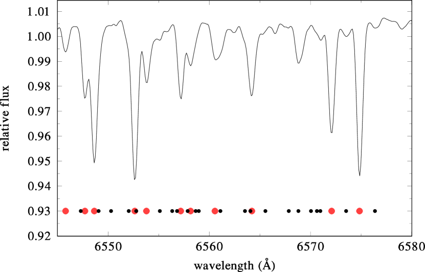
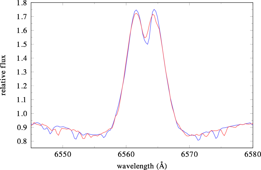
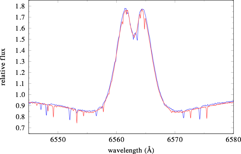
Figure 1: Comparison of medium- and high-dispersion H$\alpha$ spectra of $\beta$ CMi from the two extrema of the heliocentric RV corrections. All spectra are on the heliocentric wavelength scale. Top: Telluric lines from the Ondřejov CCD spectra disentangled with the KOREL program. Circles at the bottom of the panel show the position of all telluric lines from the solar spectrum of Moore et al. (1966), the red ones denoting the lines with equivalent widths greater than 5 mA. Middle: Ondřejov CCD spectra: blue is from RJD 56395.3447 with the heliocentric RV correction $V=-29.1$ km s^-1, red is from RJD 55470.6614 with $V=+28.3$ km s^-1. Bottom: blue is a Canada France Hawaii Telescope spectrum from RJD 52871.1482 with $V=-28.1$ km s^-1, red is the Elodie spectrum from RJD 55871.1482 with $V=+27.1$ km s^-1.

The situation is well illustrated by the fact that in spite of great effort after the first discoveries of X-ray+Be binaries, for virtually none of the main-sequence Be stars the orbital period was found from the RVs of the Be star, see, e.g. the negative search in the large collection of photographic RVs of $\gamma$ Cas by Cowley et al. (1976).

Božić et al. (1995) were the first to demonstrate that for Be stars with a strong H$\alpha$ emission the best estimate of the true orbital motion of the Be star is the RV measured on the steep outer wings of the H$\alpha$ emission, which originates from the central, more or less axially symmetric parts of the disk around the central star. This way and using the technique of the comparison of the direct and flipped line profiles on the computer screen as it is possible in the program SPEFO (Horn et al. 1996; Škoda 1996; Krpata 2008), they obtained a sinusoidal RV curve for the Be component of $\varphi$ Per.

Using the same technique, Harmanec et al. (2000) succeeded to discover the 203$\fd$6 orbital period of $\gamma$ Cas and to demostrate its presence even in the photographic RVs by Cowley et al. (1976). Their finding was then confirmed from an independent series of H$\alpha$ spectra by Miroshnichenko et al. (2002). These authors, however, measured the RV of the H$\alpha$ outer wings by an automatic procedure. Both approaches were compared in the so far richest collection of H$\alpha$ spectra of $\gamma$ Cas by Nemravová et al. (2012), with the conclusion that the manual measurement in SPEFO provides more accurate RVs than the automatic procedure. This is probably due the fact that the measurer can avoid line-profile distortions due to numerous telluric lines and/or small flaws in the region of the H$\alpha$ line.

Harmanec et al. (2002) derived the RV curve of the Be component of V832 Cyg = 59 Cyg also from the H$\alpha$ emission wings. They noted that due to a partial filling of the broad He I lines by emission, exhibiting orbital $V/R$ changes in phase with the orbital RV changes, RVs from these, seemingly photospheric lines, give an RV curve with a larger semi-amplitude than those of the H$\alpha$ emission. Their conclusion was nicely confirmed by Peters et al. (2013), who derived the RV curves of both binary components of V832 Cyg from the UV spectra. Other H$\alpha$ RV curves were also derived for $\zeta$ Tau by Ruždjak et al. (2009) (these authors summarized all reasons, why the H$\alpha$ RV measured on the steep wings of the H$\alpha$ emission best reflects the true orbital motion of the Be component) and by Koubský et al. (2010) for o Cas.

The same approach has also been used by Dulaney et al. (2017) to derive the RV curve of $\beta$ CMi. They once more used the automatic determination of the RV from the H$\alpha$ emission wings. There is a trap, however. Desmet et al. (2010) and Harmanec et al. (2015) measured the RVs of the H$\alpha$ emission wings for two Be stars in semi-detached systems with cool, Roche-lobe filling secondaries, AU Mon, and BR CMi, respectively. They found that in both cases the RVs of the H$\alpha$ emission wings led to RV curves, which were not exactly in anti-phase with respect to the well-defined RV curves of the cool secondaries but showed some phase shift. This could be due to presence of gas flow deflected by the Coriolis force in these mass-exchaning systems and also due to the fact that the H$\alpha$ emission in both objects is only moderate, with peak intensities of less than 2.0 of the continuum level. In such situations, the RV measurements are prone to the blending effects of numerous telluric lines much more than strong emission profiles.

This is, unfortunately, also the case of $\beta$ CMi, since its H$\alpha$ emission reaches only some 60 to 80 % above the continuum level. For this particular star, there are two additonal problems. It is located near the ecliptic, which causes a RV shift of the telluric lines for full 60 km s^-1 as the Earth revolves around the Sun and it can only be observed for about half a year. In Fig. 1 we show pairs of the H$\alpha$ line profiles of $\beta$ CMi from two extremes of the telluric-line shifts for high-dispersion and high-resolution, and medium-dispersion and medium-resolution spectra at our disposal. Also shown there is the mean telluric spectrum from the numerous Ondřejov spectra disentangled with the program KOREL (Hadrava 1995, 1997, 2004). One can see how the telluric lines can fool both, the precise RV measurements, and measurements of the $V/R$ ratio.

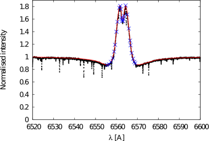
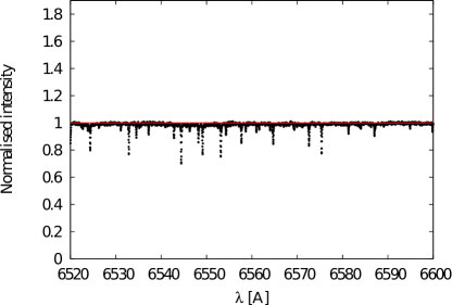
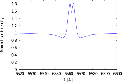
Figure 2: Cleaning one SOPHIE spectrum from telluric lines. Top: original spectrum with an artificial rectification (red) to remove the H$\alpha$ profile. Crosses denote the points where we set pseudocontinuum within the H$\alpha$ line. Middle: Clean telluric spectrum after the above artificial rectification. Bottom: Clean H$\alpha$ profile resulting from the division of the original spectrum by the clean telluric spectrum.

Being aware of this problem, Dulaney et al. (2017) applied the IRAF task telluric to get rid of them. Regrettably, they do not provide any details other than that they used spectra of rapidly rotating hot stars obtained with the same spectrograph as their spectra of $\beta$ CMi. It is not mentioned whether the spectra of rapidly rotating stars were obtained each night, when $\beta$ CMi was observed and how exactly they re-normalized them. This technique of the telluric-line removal is a delicate task. Given the fact that the reported full amplitude of RV changes of $\sim 4$ km s^-1 represent a sub-pixel resolution, it is conceivable that the removal was not complete. This suspicion seems to be supported by the fact that the residual absorption features seen at about 400, 530, and 1070 km s^-1 in Fig. 1 of Dulaney et al. (2017) clearly correspond to the strong water vapour lines at 6572.1, and 6574.8 A, and to the blend of two such lines at 6586.6 A. We do admit, however, that Dulaney et al. (2017) do not state explicitely whether the H$\alpha$ profile in their Fig. 1 corresponds to the spectrum with the telluric lines already removed or to the original one.

Figure 3: Individual quantities measured in the H$\alpha$ profiles of all spectra of Table 1 plotted vs. time (in RJD): (a) Our emission-wing RVs measured in the original spectra in SPEFO. Individual data sets are distinguished as follows: blue… DAO, black… OND R and OND C, red… best high-S/N ELODIE, FEROS, UVES, SOPHIE, and CFHT spectra, green… BESO, and brown… PUCHEROS. (b) Our emission-wing RVs measured in SPEFO in the spectra with telluric lines removed. The same notation as above. (c) Emission-wing RVs of Dulaney et al. (2017) measured by an automatic procedure by them. Since their RVs were derived via cross-correlation and cluster thus around zero, we added +9 km s^-1 to them to make the direct comparison with our RVs easier. (d) Total strength of the H$\alpha$ emission measured in our spectra as a mean of the V and R peak intensities expressed in the units of local continuum. The medium-resolution Ondřejov spectra are shown by smaller black circles than all other data.

4.1.1 RVs of the H$\alpha$ emission wings

We measured the RVs of the H$\alpha$ emission wings using two different approaches:

• Using our standard technique of the comparison of the direct and flipped line-profile images on the computer screen in the SPEFO program, we measured RVs of the steep emission-line wings of H$\alpha$ profiles on all spectra listed in Table 1, trying to avoid the parts of the profiles affected by telluric lines. All measurements were carried repeatably, at different times, not to remember the previous settings to obtain some idea about their accuracy. Moreover, we also measured a selection of telluric lines to carry out an additional correction of the zero point of the RV scale (Horn et al. 1996). The RJDs, and RVs of H$\alpha$ emission with their rms errors are provided in the first two columns of Table 4 in Appendix, while the additional RV zero point corrections and the rms errors of the mean measured RV of telluric lines are provided in the fourth and fifth column.

• Realizing that the Hermite polynomials used in SPEFO for spectra normalization can also be used for the removal of the observed H$\alpha$ profiles like it is done for the spectra of hot, rapidly rotating stars in the IRAF task telluric, we renormalized all our spectra to obtain clean spectra of telluric lines and divided the original spectra by them. In our opinion, this is a suitable approach in the given case since it uses the real strength of telluric lines and no adjustment in either the strength or velocity of the lines is needed. It also takes out the noise, so that it has a very similar effect to a low-pass filtering. We caution, however, that it can only be carried out for stars with spectral lines significantly broader than the telluric lines. The procedure worked remarkably well as it is illustrated for one spectrum in Fig. 2. We then measured the steep H$\alpha$ emission wings in the clean spectra in the same way as before. These measurements and their rms errors, based again on several repeated measurements, are given in the third column of Table 4. Finally, we also derived the strength of the H$\alpha$ emission as the mean of the strength of $V$ and $R$ peaks of the double emission profile. It is given in the sixth column of Table 4.

We started our analyses plotting the RVs of the emission wings of H$\alpha$ profiles measured by both methods versus time in Fig. 3a,b. In Fig. 3c we also plot the H$\alpha$ emission RVs obtained by Dulaney et al. (2017), and Fig. 3d we display the strength of the H$\alpha$ emission. This shows a few things.

1. There is an indication of a temporal increase of the RV to some 12 km s^-1 after RJD 51500 but it is solely based on several early Reticon spectra. It might be real since Be stars are known to show intervals of increased activity with secular RV changes. Also, as already mentioned, early photographic RVs are indicative of larger RV changes. However, without independent evidence we do not assign too much weight to it, noting that the Reticon digital convertor used only 4096 discrete levels in recording the flux.

2. It is obvious that our RV measurements are much more precise than the automatically measured RVs of Dulaney et al. (2017) and show a much lower scatter, perhaps a constant RV within the accuracy of the measurements. The real uncertainty of RV values is hard to estimate well. The rms errors of repeated setting on the emission-line wings are quite low for both methods we used. However, there can be larger external errors related, e.g., to small local inaccuracies in the dispersion relation. From the comparison of RV derived for the same spectra by two alternative approaches we conclude that the realistic error of individual RV can be something like $\pm 1$ km s^-1. Robust mean value of RVs measured in the original spectra is $8.93\pm 0.11$ km s^-1, while that for the spectra with the telluric lines removed is $9.05\pm 0.13$ km s^-1.

3. There is a very uncertain indication of a mild secular increase of the H$\alpha$ emission strength over the interval of our observations. One UVES spectrum from RJD 53334.8232, and a BESO spectrum from RJD 56929.9217 exhibit rather anomalous emission strengths. We checked the whole reduction procedure and found no problem, so we reproduce these values as they are.

Figure 4: Amplitude periodograms of several RV data sets based on the Deeming (1975) discrete Fourier transform method are shown in the left panels and the corresponding spectral windows in the right panels.

4.2 Period analyses of RVs

Using the period search based on Deeming (1975) discrete Fourier transform, we analyzed the photographic RVs published by Frost et al. (1926) and Jarad et al. (1989) (omitting two Yerkes RVs denoted as poor), RVs derived by Dulaney et al. (2017), and our SPEFO H$\alpha$ emission-line RVs for periodicity over possible binary periods from 100 to 10000 d. All correponding periodograms and window functions are in Fig. 4. We discuss these three different RV sets separately.

4.2.1 Photographic RVs

The message from older photographic spectra is somewhat unclear and confusing. RVs from the seven Yerkes spectra published by Frost et al. (1926) range from $-1$ to $+53$ km s^-1, which is too much to be explained by measuring uncertainties only. Moreover, their robust mean is $+28\pm 8$ km s^-1, substantially higher than $\sim 9$ km s^-1 invariably found from the more recent spectra. Similarly, since Jarad et al. (1989) correctly derived the 133 d orbital period for another Be star, $\zeta$ Tau, with a lower semiamplitude than what they found for $\beta$ CMi, it would not be easy to dismiss their result for $\beta$ CMi as an artefact of medium-dispersion photographic spectra. We note, however, that the full range of their RVs, 62 km s^-1, is comparable to that of the Yerkes RVs. One is, therefore, led to the suspicion that there were real RV variations of $\beta$ CMi in the past. As a check, we measured RVs of several stronger lines in the blue parts of the spectra at our disposal. We found that they do not indicate any similar large RV changes above some $2-3$ km s^-1, all RVs clustered near $9-10$ km s^-1. (We have not analyzed our blue RVs in more detail since there is no possibility to check the small possible RV zero-point shifts in regions without telluric lines.)

Not surprisingly, the period analysis of the combination of Frost et al. (1926) and Jarad et al. (1989) RVs, which are substantially separated in time, resulted in a number of one-year aliases. Formally the best periodicity is found for a period near 190 d.

To investigate these variations in a more quantitative way, we formally used the program FOTEL for binary orbital solutions and allowed different systemic velocities for the two data sets. RVs denoted as good in Frost et al. (1926) were given weight 0.5, and those denoted fair weight 0.3, while the weights of all Jarad et al. (1989) RVs were set to 1.0. The following elements led to a fit with lowest rms of 4.65 km s^-1 for Frost et al. (1926) RVs, and 6.91 km s^-1 for the Jarad et al. (1989) RVs:

$P=189\fd 917\pm 0\fd 017$,

$T_{\rm periast.}={\rm RJD}~{}31989.9\pm 2.8$,

$e=0.54\pm 0.11$, $\omega=302^{\circ}\pm 14^{\circ}$,

$K=24.4\pm 3.6$ km s^-1,

$\gamma_{\rm Frost\,et\,al.}=27.9\pm 2.4$ km s^-1,

$\gamma_{\rm Jarad\,et\,al.}=11.2\pm 1.5$ km s^-1.

The RV curve corresponding to this fit is plotted in Fig. 5.

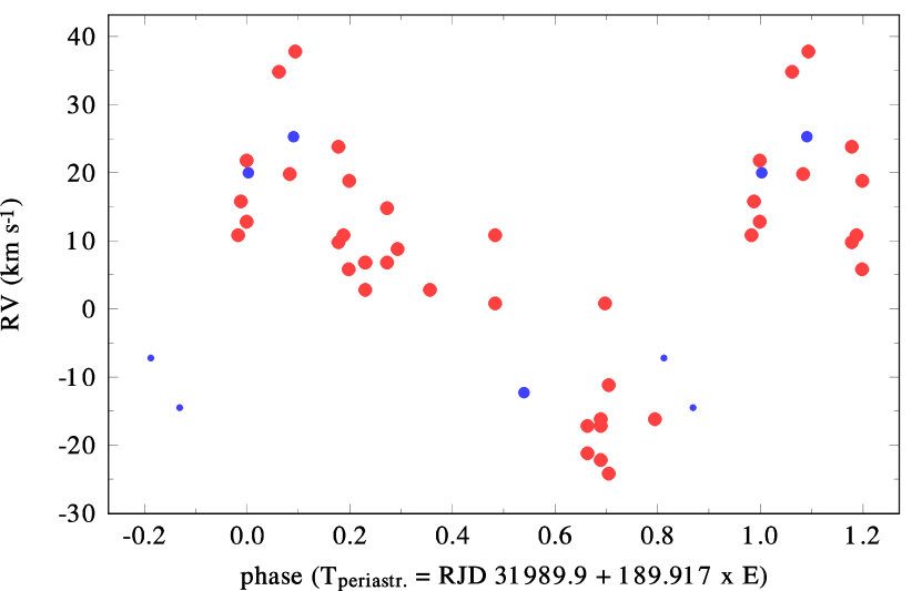
Figure 5: Plot of RVs published by Frost et al. (1926) (blue circles) and Jarad et al. (1989) (red circles) vs. phase of the 189$\fd$917 period. Frost et al. (1926) RV denoted as “fair” are shown by smaller symbols.

Figure 6: A plot of Dulaney et al. (2017) H$\alpha$ emission RVs vs. phase of the 336$\fd$95 period (top) and for their original period of 170$\fd$4 (bottom). The same epoch of maximum RV, RJD 52001.2, was adopted as phase zero in both plots.

4.2.2 Dulaney et al. (2017) emission-wing RVs

The periodogram of Dulaney et al. (2017) RVs indicate the highest peaks at frequencies of 0.00016869 c d^-1, and 0.0029678 c d^-1. The latter corresponds to a period of 336$\fd$95, i.e. roughly twice the period reported by them. Moreover, we note that the difference of both frequencies corresponds to the frequency of one year. The phase plot for the 336$\fd$95 period is in Figure 6. This phase curve looks certainly less scattered than the plot of the same RVs vs. phase of the 170$\fd$4 period advocated by Dulaney et al. (2017), but it can simply represent a one-year alias of the period of one year over the interval covered by their data.

Figure 7: Phase plots of our H$\alpha$ emission-line RVs, both from the original spectra and from the spectra after removal of telluric lines, for the “period” of 160$\fd$86 found as the best one from the original spectra, and for 137$\fd$56 found from the spectra after the telluric-line removal.

4.2.3 Our H$\alpha$ emission RVs

We derived the periodograms for both, the RVs from the original spectra and from the spectra after the removal of telluric lines (see Fig. 4). It is seen that different best-fit frequencies of 0.0062166 c d^-1, and 0.0072695 c d^-1were detected for the original, and telluric-corrected spectra, respectively. These correspond to “periods” of 160$\fd$86, and 137$\fd$56. The phase plots for both these “periods” and both sets of RVs are in Fig. 7. One can see that neither phase curve is very convincing. Moreover, it is obvious that no strong peak was detected near frequency of 0.00587 c d^-1, which corresponds to the period of 170$\fd$4 reported by Dulaney et al. (2017) – cf. Fig. 4. We thus re-iterate our conclusion that our RVs do not indicate RV variability.

5 Could the presence of telluric lines confuse the automated RV measurements?

RVs are often measured using various automatic routines or pipelines. As already mentioned, there is a large number of telluric lines in the H$\alpha$ region – see Fig. 1. If these lines are not removed properly, they could possibly affect or even confuse the automatic procedures that measure the RVs. In the course of the year the positions of the telluric lines with respect of the line profile change periodically. If the telluric lines are not removed correctly, they could easily cause apparent periodic RV changes.

To investigate how significant the line blending of numerous telluric lines with the observed H$\alpha$ profile can be, we carried out tests on artificially created data for the observing times of the Ritter spectra.

We realized that the spectral resolution of the DAO spectra is similar to that of the Ritter spectra studied by Dulaney et al. (2017). We therefore used this richest and longest homogeneous series, covering the red spectral region, and applied the KOREL disentangling (Hadrava 2004, and references therein) to them. We assumed a constant spectrum of $\beta$ CMi (simulating it as a very long-period orbit with virtually zero semi-amplitude of RV changes) and we also disentangled the spectrum of telluric lines, allowing for their time variability. The resulted spectra are shown in Fig. 8.

Figure 8: Top: The mean disentangled DAO red spectrum of $\beta$ CMi, with several clearly visible spectral lines: absorption lines of the Si II  6347&6371 A doublet, double emission lines of Fe II  6456 and Fe II  6519&6525 A blend, H$\alpha$ emission, and He I  6678 A absorption. Bottom: The mean disentangled spectrum of telluric lines.

Then we multiplied the mean DAO stellar spectrum in the neighbourhood of H$\alpha$ by the mean spectrum of telluric lines, each time shifted in RV to the respective values of the heliocentric RV corrections. The multiplication is a better justified operation because the telluric spectral lines do not have a continuum, thus the strength of the telluric line which absorbs at stellar continuum will be different from the strength of the same line absorbing in the strong stellar line (see the discussion on this topic in Hrudková & Harmanec 2005 and Hadrava 2006). We omitted the spectrum with RJD 52975.8496 with tabulated H$\alpha$ emission RV of $-1.88$ km s^-1 in the electronic table of Dulaney et al. (2017), since this RJD is out of the increasing order of RJDs and the same value repeats a few lines later with a RV of $-3.41$ km s^-1. Then we imported all artificial spectra to SPEFO and measured their $V/R$ ratio. We also measured RVs on the steep wings of the H$\alpha$ line using an automatic procedure, namely a simplified double-slit method, commonly used in solar physics. This method utilises two artificial slits placed in a fixed distance in wavelength on the steep wings of the spectral line. The double slit is then moved across the line profile to balance the transmission through both slits. The position of the double slit then corresponds to the RV of the spectral line. The method is known to be performing well on symmetric lines, which roughly corresponds to our case.

In other words, we used an H$\alpha$ profile with constant RV and $V/R$ ratio. We found that the $V/R$ ratio of the disentangled DAO H$\alpha$ profile differs a bit from one, having $V/R=0.99792$. To test the hypothesis that the real $\beta$ CMi profile has $V/R=1.0$ sharply, we multiplied all $V/R$ ratios measured on the simulated spectra by an inverse factor of 1.00208.

We underline that we are aware that such simulation cannot reproduce the observed spectra well enough. Not only that our simulated spectra are essentially noiseless in contrast to the observed ones but the strength of the telluric lines in the real spectra certainly varies from one to another, while our simulation used a mean telluric spectrum of constant intensity. Yet, our results are very illuminating and clearly show that the blending of the H$\alpha$ profile with telluric lines, which are changing their positions with time during the year lead to apparent RV and $V/R$ changes, especially when the peak intensities of the emission line are modest, not exceeding the continuum level by two to three times.

We first discuss the results for the $V/R$ ratio. We note that the times of observations of the Ritter spectra are such that the vast majority of them have heliocentric RV corrections from $-29$ to $+3$ km s^-1 and there are only 17 spectra (out of 123), which have heliocentric RV corrections larger than +15. We suspect that one consequence of this fact is that almost all $V/R$ ratios measured by Dulaney et al. (2017) are larger than one. In Fig. 9 we compare the phase plot of the $V/R$ ratios measured by Dulaney et al. (2017) on real Ritter spectra with that for the artificially created spectra. We note that our result for artificially created spectra shows a remarkable agreement with the real Ritter spectra as far as the range of the $V/R$ ratios is concerned. Since our modelling used a constant H$\alpha$ profile with $V/R$ tuned to one, this seems to constitute an indirect but quite compelling argument that the $V/R$ changes derived by Dulaney et al. (2017) are still partly affected by spurious effects due to blends with the telluric lines.

Figure 9: Phase plots of the $V/R$ ratio of the double H$\alpha$ emission for the ephemeris of Dulaney et al. (2017) $T_{\rm max.RV}=RJD~{}52001.2+170\fd 4\times E$. Top: Measurements of Dulaney et al. (2017) on the Ritter spectra; Bottom: Simulation of Ritter spectra based on combined disentangled DAO line profile of H$\alpha$ multiplied by the spectrum of telluric lines (see the text for details).

Figure 10: Phase plots of the $V/R$ ratio (left columns) and RV (right columns) of the H$\alpha$ emission wings measured on the simulated Ritter spectra. The phase diagrams are plotted for the periods of half of the tropical year (upper row) and the period of one tropical year (bottom row). In panel (d), the gray points were calculated for simulation covering every day over one tropical year, whereas the black points represent the dates of Ritter spectra.

We carried out a period analysis of the $V/R$ ratio to find out that the best period is one half of the tropical year. The corresponding phase plot is in Fig. 10a.

We also carried out period analyses of RVs of the H$\alpha$ emission wings measured by the automatic procedure. The best fit was also obtained for one half of the tropical year – see Fig. 9b. We note that the phase curves of RVs measured by the automatic method we used are very smooth. We explain this by the fact that the simulated spectra are noiseless and the slit method inevitably feels the variable blending on both line wings. We note that the RV curve shows a strange behavior in phases from 0.1 to 0.3 . This corresponds to a large discontinuity at the same phase seen in phase curve of RVs in Fig. 10b, which is caused by the gap in observations in autumn, when the star was below the horizon at night (this gap is demonstrated in Fig. 10d).

A related question is why does the periodic analysis prefer the period of one half of the tropical year to the full tropical year, which should naturally be present in the simulated spectra since it was introduced by our simulation. As we demonstrate in Fig. 10d, the simulated spectra indeed have one-tropical-year periodicity with two half-year waves of different amplitudes (the gray points that were computed for automatic measurements covering one tropical year). In all probability, it is a consequence of asymmetric distribution of stronger telluric lines with respect to the laboratory wavelength of the H$\alpha$ line. As seen in Fig. 10d, the Ritter spectra were almost exclusively exposed in such dates that their positions cover preferrably the wave with a larger amplitude. A period search seeking for a single-wave RV curve then naturally gets confused due to this selection effect and finds a half-tropical-year period as the best one describing the periodicity in the data. Finally, we note that the RVs from our simulated spectra have a phase of maximum RV identical to that found by Dulaney et al. (2017) in their real measurements. This indicates that the period suggested by them might indeed be spurious due to residual telluric contamination.

We conclude that the spurious effects due to blending of the H$\alpha$ profile of $\beta$ CMi with telluric lines, varying in position and strength, are inevitable. This represents a serious warning that any periods close to a year or half of it must be considered with caution.

6 Period analysis of light changes with wavelets

The star was almost continuously monitored by the Canadian MOST satellite for more than 39 days with a very high cadence (an average separation between the consecutive measurements is about 8 minutes – see Fig. 11a). Such a data set allows to study photometric periods and their evolution.

The standard methods (for instance a Fourier analysis) were used to analyse the same data set in the past (e.g. Saio et al. 2007). A number of short periods was identified and interpreted as evidence for non-radial pulsations. The classical methods do not allow to learn about the evolution of the periods over the interval of observations.

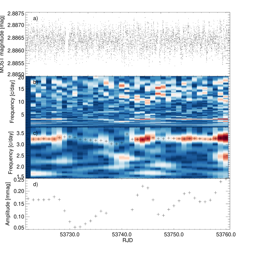
Figure 11: Period analysis of MOST photometry of $\beta$ CMi (a) The observations, (b) the WWZ spectrum, (c) the zoom in the range of the dominant frequency with the peak identified, and (d) its amplitude over the interval of observations.

In order to study such a case we use the method that is based on the wavelet transform (e.g. Morlet et al. 1982). For details of the method and its trial application, see Švanda & Harmanec (2017). The wavelet transform can provide a good time resolution for high-frequency signals and a good frequency resolution for low-frequency ones. That is a property well suited for real signals. The wavelet transform is thus a convenient method for the analysis of periodic signals with cycle lengths, amplitude and/or phase, which evolve with time. If applied to irregular data sets, the wavelet transform responds to irregularities rather than to actual changes in the parameters of the signal. Foster (1996) introduced a wavelet Z-transform (WWZ) that corrects the amplitude of the detected period to the number of points available to properly describe the given periodicity, thereby dealing with gaps and irregularities in the dataset. The WWZ approach represents the principal method to investigate the periodicities seen in the MOST photometry.

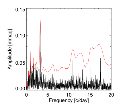
Figure 12: An average periodogram obtained from WWZ analysis (as a time average of Fig. 11b – the red line) compared to the PERIOD04 periodogram (black curve).

Figure 13: Double-wave light curves constructed from the MOST photometry for five non-overlapping intervals. The corresponding intervals of RJDs and local values of the period are given for each plot. The left panels correspond to locally derived values of the period while the right ones are for the constant mean period. On abscissa, the phase calculated for each local value of the period, with phase zero set always at RJD 53740, is given for each plot.

The overall wavelet spectrum is plotted in Fig. 11b. It can be seen that except for the enhanced power at around 3.25c d^-1, none of the detected periods is stable over the whole interval of observations. From time to time, a strong power near 12 c d^-1, and 17 c d^-1 appears and disappears again. The averaged periodogram over the whole interval of observations is plotted in Fig. 12 in comparison with a periodogram obtained with the program PERIOD04 based on the Deeming (1975) method (Lenz & Breger 2004). The resolution in frequency is poorer for WWZ spectrum, which is a natural property of this method because for time instant only a limited interval of observations is considered. Nevertheless, all important frequencies below 5 c d^-1 are detected by both approaches. The two differ for higher frequencies, where the peak-width is much broader for the WWZ spectrum than for the PERIOD04 spectrum. Yet, the PERIOD04 peaks around 11 c d^-1, 13 c d^-1, 15 c d^-1 and 17 c d^-1 can be identified in the average WWZ periodogram as well as transients. When looking at the full WWZ spectrum in Fig. 11b one sees that these high-frequency periods were detected only episodically in the second half of the observational interval and were virtually absent in the first half.

The strongest periodicity around 3.25 c d^-1 was quite stable over the whole interval (see Fig. 11c) with the cycle length of $0.307\pm 0.004$ days and underwent smooth changes around its mean value. Its significance (amplitude) also evolved slightly in time (Fig. 11d), this periodicity was on average responsible for the observed photometric changes with the amplitude of 0${}^{\rm m}\!\!.$00014$\pm$0${}^{\rm m}\!\!.$00005. The exception is seen in an interval between RJD 53738 and 53742, where a different cycle of length about 2.4 c d^-1 with a secular evolution dominates the spectrum. Cycles of a similar length are episodically present also on other dates. From seeing the WWZ spectrum in Fig. 11c one could even track a non-monotonic secular evolution of such cycle.

Saio et al. (2007) claimed to detect two separate peaks in the spectrum with frequencies $3.257\pm 0.001$ c d^-1 and $3.282\pm 0.004$ c d^-1 that they interpreted as a coupling between the rotation of the star and the non-radial $g$-mode pulsations. They further reported weak frequency peaks with values of $3.135\pm 0.006$ c d^-1 and $3.380\pm 0.002$ c d^-1. The detection of separate peaks is not confirmed by the WWZ method. The multiperiodicity of the close periods, when typically the $g$-modes create frequency groups that are also observed on Be stars (Rivinius et al. 2016), manifest themselves as beat-like structures in the wavelet spectrum at a fixed frequency (cf. also Pápics et al. 2017). The wavelet spectrum of $\beta$ CMi does not contain such features and it is qualitatively different from the typical wavelet spectrum of pulsating Be stars (see Rivinius et al. 2016, and their Figs. 2, 4, and 6).

Instead of distinct multiperiodic representation we observe a slowly changing value of the dominant frequency oscillating about the value of $\sim$3.257 c d^-1. If such an evolving signal is analysed using the standard periodogram methods, the method will find a solution in a sum of periodic signals with arbitrary periods. Even though a representation of a times series with a set of periodic signals may be sufficient for some applications, such a representation does not reveal possible real physical changes. We do not claim that $\beta$ CMi is not a pulsating star, we only demonstrate that there is no clear evidence of pulsations in the MOST observations.

There has been a long debate about the nature of the low-amplitude (multi?)-periodic light variations observed for many Be stars. Since Harmanec (1984) called attention to the fact that these variations often occur with a double-wave curve and this was confirmed on a larger sample of stars by Balona & Engelbrecht (1986), small-amplitude periodic light changes were found for a number of Be stars. While P. Harmanec and L.A. Balona, among others, advocated the rotational modulation of the stars in question or their circumstellar envelopes, investigators like C.T. Bolton, J.R. Percy, D. Baade or G.A.H. Walker with their collaborators advocated interpretation in terms of non-radial pulsations. Readers are referred to, e.g. Baade & Balona (1994) and many other papers by the above authors or to a more recent repetition of the debate (e.g. Balona 2013; Rivinius 2013; Rivinius et al. 2013).

Harmanec (1998) analyzed extended series of observations of $\omega$ CMa, interpreted as non-radial pulsator by Baade, and showed that the $O-C$ analysis of its RV changes with the 1$\fd$37 period indicate mild secular cyclic variations of this period, possibly related to the strength of the H$\alpha$ emission. He also showed that a Fourier analysis of all RVs can misinterpret a single periodicity with mildly variable period as multiperiodicity of several close periods. It was also found that the shape of the periodic light variations can change gradually, even within one season, from double-wave to single-wave shape (cf., e.g. Cuypers et al. 1989; Balona et al. 1992; Harmanec et al. 1987). This also complicates the period analysis based on Fourier analyses.

In the case of $\beta$ CMi , the dominant period changing in time also represents the real changes of the light curve. To demonstrate this effect, we split the whole 39-day interval into 5 intervals of equal length. For each interval we determined the local value of the dominant period around 3.257 c d^-1 and construct the light curve as a function of phase. We soon found that phase plots of the data with a half of this frequency define a double-wave light variation, with unequal minima and maxima. For a better clarity, the light curves were binned with a binsize of $0.025$ in phase, the sampling in phase has a step of $0.01$.

The light curves from individual data subsets plotted in the left panels of Fig. 13 show that the shape of the light curve varies indeed from one subset to another. The spread of the points around the mean curve is larger for the second and third subsets since, as it is evident from Fig. 11c, in those time intervals the value of the dominant period is changing rapidly. On the other hand, in the first, fourth and fifth time subset the period was quite stable, which led to a “cleaner” appearance of the light curve.

The plots also demonstrate that the choice of twice longer period then the dominant local period detected with the wavelet analysis was a correct one. The depths of the two maxima and minima are clearly different. Furthermore the phase shift of the curves also varies from one subset to another. As mentioned above, such a behaviour is characteristic for rapid light changes of other Be stars, too – see, for instance, the rapidly changing light curve of the archetype rapidly variable B6e star $o$ And (Harmanec et al. 1987; Sareyan et al. 1998, 2002) and for a number of other Be stars (Cuypers et al. 1989; Balona et al. 1992). That all is consistent with the rotational modulation and physical changes taking place and inconsistent with the multiperiodic oscillations.

On the other hand the variations of the peak frequency in the five intervals is small, thus it is almost impossible to convincingly show the effects of the period determination on the phase light curves. To show this weak effect, we plotted the same data for a constant period of 0$\fd$617 the right panels of Fig. 13. The differences between the corresponding panels of Fig. 13 are small and probably beyond statistical significance.

In passing, we admit that in view of the very low amplitude of the light changes, our interpretation is only tentative. The majority of investigators currently favours the hypothesis of non-radial pulsations to explain the rapid light- and also line-profile changes of Be stars.

7 Probable physical properties

There is actually a rather large range of uncertainty of the basic physical properties of $\beta$ CMi.

We used the PYTERPOL program of J.A. Nemravová (see Nemravová et al. 2016, for the most detailed description) that interpolates in a precalculated grid of synthetic stellar spectra sampled in the effective temperature, gravitational acceleration, and metallicity. The synthetic spectra are compared either to individual observed spectra or to the disentangled ones for one, two or more components of a multiple system (normalised to the joint continuum of all bodies) and the initial parameters are optimised by minimisation of $\chi^{2}$ until the best match is achieved. In our case, we used the blue parts of the high-S/N spectra in three regions: $4000-4190$ A, $4250-4420$ A, and $4440-4600$ A. We fitted the individual spectra and as another trial, we also disentangled the spectra with KOREL and fitted the disentangled spectrum. The result is summarised in Table 2. The difference between the two fits probably characterises the real uncertainty of the values obtained.

For comparison, Frémat et al. (2005) derived $T_{\rm eff}$ = $11772\pm 344$ K, log $g$ = $3.811\pm 0.062$, and $v$ sin $i$ $230\pm 14$ km s^-1, while Slettebak (1954) obtained $v$ sin $i$ $=260$ km s^-1 . Reproducing the optical and UV spectral energy distribution, Wheelwright et al. (2012) concluded that the disk is in Keplerian rotation and seen under an inclination of about $45^{\circ}-50^{\circ}$. They adopted $T_{\rm eff}$ = 12000 K and log $g$ = 4.0 as typical for a B8e star and estimated the equatorial radius of the star of 4.68 R_⊙, $A_{\rm V}=0$${}^{\rm m}\!\!.$05, and polar temperature of 15000 K.

Table 2: Estimates of the radiative paramaters of $\beta$ CMi from the blue spectra at our disposal with the program PYTERPOL. Results of the fit for individual spectra, and for the KOREL disentangled spectrum are tabulated. The solar composition was assumed.

Quantity	Individual spectra	KOREL
$T_{\rm eff}$ (K)	12560	13010
log $g$ [cgs]	4.20	4.35
$v$ sin $i$ (km s-1)	260	266

There is no Gaia DR2 release parallax of $\beta$ CMi since the star is too bright. The most accurate parallax is from the Hipparcos revised reduction (van Leeuwen 2007): $p=0\farcs 02017\pm 0\farcs 00020$. Combined with the calibrated standard $U\!B{}V$ photometry from Hvar ($V=2$${}^{\rm m}\!\!.$890, B V$=-0$${}^{\rm m}\!\!.$101, U B$=-0$${}^{\rm m}\!\!.$268) and $A_{\rm V}=0$${}^{\rm m}\!\!.$05 (Wheelwright et al. 2012), one obtains $V_{0}=2$${}^{\rm m}\!\!.$84, and M${}_{\rm V}=-0$${}^{\rm m}\!\!.$64. Using the two extreme values of $\log$$T_{\rm eff}$ , 4.071 (Frémat et al. 2005) and 4.114 (from the PYTERPOL fit of KOREL disentangled blue spectrum) and bolometric corrections from Flower (1996), one obtains the mean stellar radius of 3.83 R_⊙, or 3.52 R_⊙, respectively. This is in a broad agreement with modelling results. Klement et al. (2015) obtained the equatorial and polar radii of 4.17 R_⊙, and 2.8 R_⊙, respectively, while Wheelwright et al. (2012) got 4.68 R_⊙, and 3.55 R_⊙. Their results imply the mean radii of 3.42 R_⊙, and 4.07 R_⊙. For completeness, mean radii of normal stars for the two extreme values of $T_{\rm eff}$ would be 2.45, and 2.65 R_⊙ (Harmanec 1988).

Our $v$ sin $i$ of $\sim 260$ km s^-1 combined with the published values of equatorial radius of 4.68 R_⊙ and 4.20 R_⊙ and assuming that the 0$\fd$617 period is the stellar rotational period would lead to the inclination of the rotational axis of $42^{\circ}\!\!.7$, and $49^{\circ}\!\!.0$, respectively.

Assuming that the circumstellar disk lies in the stellar equatorial plane Klement et al. (2015) obtained an inclination of 43^∘ and Wheelwright et al. (2012) estimated the range of inclinations $45^{\circ}-50^{\circ}$. Our identification of the 0$\fd$617 period with the stellar rotational period is therefore quite consistent with these pieces of information.

8 Conclusions

Our detailed analyses presented in previous sections demonstrated that the spectroscopic binary nature of $\beta$ CMi with an orbital period of 170$\fd$4 could not be confirmed. The star can still be a binary (as conjectured from the truncation of its circumstellar disk by Klement et al. 2015) but there is currently no direct proof of it, based on periodic RV changes.

The discussion of RVs from photographic spectra in sect. 4.2.1 indicates that there could be time intervals in the past when the RV was varying within a rather large range of values, perhaps due to transient asymmetries in the circumstellar disk. We remind that $V/R=1.17$ was found on an H$\alpha$ profile from March 1953 published by Underhill (1953).

From the wavelet analysis of the precise MOST satellite photometry we conclude that there is only one stable (maybe slightly variable) period of low-amplitude light changes, 0$\fd$617. We tentatively identify it with the star’s rotational period.

Appendix A Appendix Tables with individual RVs and spectrophotometric quantities

We provide here individual RVs with RJDs derived by us for the Yerkes photographic spectra in Tab. 3 and also individual RVs and spectrophotometric quatities for our H$\alpha$ spectra - see Tab. 4. We tabulate the peak intensities $I_{V}$ and $I_{R}$ measured in the units of the local continuum level, their average and ratio, and the central intensity of the H$\alpha$ absorption core $I_{\rm c}$. Individual spectrographs are identified in the last column “Spg. No.” by numbers they have in Tab. 1.

Table 3: RVs (in km s^-1) from Yerkes photographic spectra published by Frost et al. (1926)

RJD	RV
16796.9717	47.90
18670.7214	13.40
19022.7829	-1.30
19029.7902	44.20
19039.8355	20.70
19092.6680	53.20
19367.8188	15.60

Table 4: Individual RV (in km s^-1) and line-strength measurements in the H$\alpha$ spectra at our disposal.

RJD	RVem.	RV${}_{\rm em.}^{\rm clean}$	dRVzero	rms${}_{\,\rm telur.l.}$	$(I_{V}+I_{R})/2$	Spg. No.
49745.8724	8.44$\pm$0.22	8.90$\pm$0.09	-0.36	0.16	$1.7095\pm 0.0095$	1
49745.8813	8.42$\pm$0.17	8.24$\pm$0.08	0.15	0.12	$1.7065\pm 0.0035$	1
51567.4879	7.15$\pm$0.40	5.64$\pm$0.16	-0.56	0.75	$1.6030\pm 0.0010$	2
51589.4298	12.43$\pm$0.03	13.01$\pm$0.09	2.02	0.28	$1.6795\pm 0.0015$	2
51641.2949	12.76$\pm$0.03	14.10$\pm$0.51	3.79	0.95	$1.6810\pm 0.0130$	2
51655.3022	12.21$\pm$0.15	12.09$\pm$0.24	1.87	0.20	$1.6785\pm 0.0085$	2
51661.3168	11.79$\pm$0.22	11.77$\pm$0.09	2.67	0.19	$1.6885\pm 0.0085$	2
52229.5462	10.58$\pm$0.70	8.29$\pm$0.18	-0.07	0.27	$1.6735\pm 0.0065$	3
52234.5702	8.83$\pm$0.03	9.14$\pm$0.06	-0.95	0.46	$1.6825\pm 0.0185$	3
52234.5821	9.11$\pm$0.29	8.76$\pm$0.12	-0.93	0.36	$1.6895\pm 0.0165$	3
52362.3431	8.46$\pm$0.14	8.91$\pm$0.08	-0.01	0.07	$1.7775\pm 0.0035$	4
52706.7670	9.31$\pm$0.11	9.56$\pm$0.10	1.28	0.19	$1.7910\pm 0.0090$	1
52706.7811	8.55$\pm$0.22	8.43$\pm$0.10	1.42	0.17	$1.7860\pm 0.0020$	1
52706.7964	9.22$\pm$0.22	9.39$\pm$0.06	1.12	0.25	$1.7935\pm 0.0025$	1
52749.3933	8.09$\pm$0.38	9.21$\pm$1.32	-1.00	0.30	$1.7645\pm 0.0075$	3
52750.3686	10.60$\pm$0.03	9.23$\pm$0.67	-0.70	0.30	$1.7700\pm 0.0010$	3
52770.6970	8.40$\pm$0.17	8.94$\pm$0.15	4.21	0.11	$1.7420\pm 0.0220$	1
52770.7018	8.29$\pm$0.17	8.34$\pm$0.10	4.53	0.12	$1.7870\pm 0.0040$	1
52771.6852	9.28$\pm$0.11	8.71$\pm$0.09	2.76	0.11	$1.7775\pm 0.0035$	1
52983.4974	9.04$\pm$0.29	9.59$\pm$0.09	-0.43	0.31	$1.7585\pm 0.0205$	3
53011.7141	8.69$\pm$0.15	7.99$\pm$0.11	-0.95	0.09	$1.7880\pm 0.0130$	5
53012.6330	8.37$\pm$0.21	8.96$\pm$0.17	-0.24	0.05	$1.8000\pm 0.0070$	5
53028.6014	9.09$\pm$0.03	9.39$\pm$0.10	-0.47	0.47	$1.7715\pm 0.0085$	3
53079.7813	9.26$\pm$0.33	9.20$\pm$0.09	0.87	0.12	$1.7885\pm 0.0115$	1
53097.3956	9.16$\pm$0.52	9.85$\pm$0.12	0.55	0.35	$1.7720\pm 0.0060$	3
53097.3993	8.69$\pm$0.61	10.18$\pm$0.08	0.38	0.41	$1.7780\pm 0.0020$	3
53105.7900	8.02$\pm$0.22	8.06$\pm$0.09	1.58	0.14	$1.7830\pm 0.0120$	1
53134.7252	8.66$\pm$0.34	9.17$\pm$0.06	0.25	0.19	$1.7975\pm 0.0025$	1
53261.0526	8.50$\pm$0.17	8.62$\pm$0.10	1.24	0.14	$1.7395\pm 0.0025$	1
53274.0536	8.36$\pm$0.17	8.25$\pm$0.08	1.48	0.13	$1.7590\pm 0.0030$	1
53334.8232	8.10$\pm$0.17	7.90$\pm$0.09	0.75	0.06	$1.8925\pm 0.0055$	6
53334.8527	7.64$\pm$0.07	7.44$\pm$0.18	1.17	0.04	$1.8250\pm 0.0030$	6
53385.9364	9.26$\pm$0.11	8.81$\pm$0.06	0.45	0.14	$1.7720\pm 0.0100$	1
53406.8866	9.67$\pm$0.19	9.62$\pm$0.09	0.50	0.19	$1.7765\pm 0.0015$	1
53469.7531	9.45$\pm$0.11	9.64$\pm$0.09	0.57	0.14	$1.7720\pm 0.0060$	1
53470.7984	9.21$\pm$0.11	9.33$\pm$0.10	0.40	0.13	$1.7890\pm 0.0030$	1
53638.0548	8.43$\pm$0.11	9.35$\pm$0.13	0.03	0.16	$1.7440\pm 0.0010$	1
53638.0566	8.54$\pm$0.11	8.56$\pm$0.12	-0.06	0.15	$1.7460\pm 0.0040$	1
53655.0693	9.53$\pm$0.17	9.54$\pm$0.10	0.12	0.14	$1.7535\pm 0.0085$	1
53681.0415	8.94$\pm$0.30	9.23$\pm$0.10	0.19	0.18	$1.7735\pm 0.0005$	1
53791.8117	9.15$\pm$0.34	9.11$\pm$0.10	-0.41	0.17	$1.7805\pm 0.0065$	1
53814.7848	9.18$\pm$0.11	10.06$\pm$0.10	-0.78	0.14	$1.7675\pm 0.0035$	1
53814.7867	9.30$\pm$0.17	9.69$\pm$0.09	-0.96	0.19	$1.7590\pm 0.0030$	1
54004.0644	8.58$\pm$0.23	8.72$\pm$0.09	-0.29	0.11	$1.7545\pm 0.0055$	1
54044.9503	8.93$\pm$0.17	9.05$\pm$0.09	0.69	0.12	$1.7555\pm 0.0035$	1
54107.0056	8.87$\pm$0.17	8.93$\pm$0.10	-0.61	0.16	$1.7680\pm 0.0120$	1
54108.5620	8.48$\pm$0.02	8.28$\pm$0.08	-1.04	0.43	$1.7495\pm 0.0225$	3
54108.5657	8.54$\pm$0.04	8.04$\pm$0.09	-0.38	0.41	$1.7470\pm 0.0230$	3
54169.8236	8.36$\pm$0.23	8.92$\pm$0.13	-0.42	0.18	$1.7865\pm 0.0015$	1
54401.0389	9.93$\pm$0.17	8.45$\pm$0.08	0.32	0.42	$1.7420\pm 0.0040$	1
54423.7029	7.72$\pm$0.24	7.81$\pm$0.05	-0.09	0.06	$1.8055\pm 0.0035$	7
54423.7047	7.54$\pm$0.25	8.21$\pm$0.05	-0.06	0.07	$1.8090\pm 0.0030$	7
54443.0654	7.95$\pm$0.11	8.64$\pm$0.09	-0.12	0.22	$1.7645\pm 0.0105$	1
54518.8122	9.17$\pm$0.17	9.56$\pm$0.09	-0.05	0.19	$1.7770\pm 0.0050$	1
54519.6421	9.42$\pm$0.20	9.29$\pm$0.10	0.16	0.19	$1.7825\pm 0.0025$	1
55320.4961	9.65$\pm$0.27	11.02$\pm$0.11	3.99	0.12	$1.8030\pm 0.0020$	8
55470.6614	8.84$\pm$0.05	8.67$\pm$0.09	0.18	0.46	$1.7210\pm 0.0030$	3
55829.6123	9.45$\pm$0.29	9.54$\pm$0.15	0.08	0.45	$1.6800\pm 0.0130$	3
55867.8024	8.97$\pm$0.14	10.06$\pm$0.15	-3.00	0.09	$1.8090\pm 0.0090$	8
55871.1482	8.82$\pm$0.06	8.50$\pm$0.10	0.03	0.06	$1.7655\pm 0.0025$	9
55877.1439	8.77$\pm$0.14	8.60$\pm$0.09	0.07	0.05	$1.7625\pm 0.0025$	9
55976.5869	10.02$\pm$0.27	9.67$\pm$0.13	-3.46	0.05	$1.7365\pm 0.0035$	8
55977.6398	9.81$\pm$0.06	10.13$\pm$0.12	-5.20	0.06	$1.7235\pm 0.0035$	8
56323.7302	7.09$\pm$0.21	8.46$\pm$0.09	-4.12	0.07	$1.7795\pm 0.0125$	8
56332.3951	7.51$\pm$1.17	8.10$\pm$0.51	0.01	0.58	$1.7395\pm 0.0065$	3
56350.6653	8.96$\pm$0.14	8.79$\pm$0.12	0.35	0.15	$1.8260\pm 0.0160$	10
56354.4928	8.32$\pm$0.04	8.92$\pm$0.12	-0.52	0.38	$1.7515\pm 0.0025$	3
56366.3279	8.16$\pm$0.03	7.70$\pm$0.09	1.24	0.40	$1.7480\pm 0.0020$	3
56395.3447	10.34$\pm$0.03	9.60$\pm$0.19	-0.71	0.27	$1.7500\pm 0.0020$	3
56606.5390	10.30$\pm$0.04	10.05$\pm$0.09	0.70	0.53	$1.7365\pm 0.0055$	3
56613.8631	7.77$\pm$0.07	8.38$\pm$0.05	-1.53	0.05	$1.8375\pm 0.0035$	8
56647.8767	8.09$\pm$0.27	8.02$\pm$0.10	-0.32	0.09	$1.8175\pm 0.0125$	8
56648.3346	10.01$\pm$0.18	9.81$\pm$0.44	1.04	0.32	$1.7085\pm 0.0365$	3
56681.6714	8.34$\pm$0.04	8.60$\pm$0.09	-0.07	0.06	$1.8420\pm 0.0120$	8
56712.2316	9.36$\pm$0.22	9.79$\pm$0.50	-0.30	0.37	$1.7550\pm 0.0100$	3
56929.9217	9.70$\pm$0.07	8.67$\pm$0.11	0.54	0.12	$1.7020\pm 0.0050$	8
56962.8833	8.98$\pm$0.03	9.73$\pm$0.06	1.02	0.08	$1.8095\pm 0.0105$	8
57078.5964	10.11$\pm$0.45	8.42$\pm$0.24	0.99	0.36	$1.8755\pm 0.0335$	10
57080.5584	9.73$\pm$0.24	9.77$\pm$0.15	1.08	0.30	$1.8290\pm 0.0030$	10
57396.5672	9.77$\pm$0.26	10.02$\pm$0.08	0.28	0.42	$1.7460\pm 0.0150$	3
57443.2592	9.73$\pm$0.02	10.07$\pm$0.63	1.18	0.53	$1.7500\pm 0.0080$	3
58163.2564	9.15$\pm$0.07	8.72$\pm$0.30	-0.97	0.53	$1.7770\pm 0.0040$	3
58173.4674	9.40$\pm$0.03	9.95$\pm$0.11	-2.01	0.61	$1.7620\pm 0.0040$	3
58198.3383	9.92$\pm$0.26	10.56$\pm$0.10	-0.19	0.44	$1.7635\pm 0.0055$	3

References

- Arcos et al. (2018) Arcos, C., Kanaan, S., Chávez, J., et al. 2018, MNRAS, 474, 5287, doi: 10.1093/mnras/stx3075
- Baade & Balona (1994) Baade, D., & Balona, L. A. 1994, in IAU Symposium, Vol. 162, Pulsation; Rotation; and Mass Loss in Early-Type Stars, ed. L. A. Balona, H. F. Henrichs, & J. M. Le Contel, 311
- Balona (2013) Balona, L. A. 2013, in Astrophysics and Space Science Proceedings, Vol. 31, Stellar Pulsations: Impact of New Instrumentation and New Insights, ed. J. C. Suárez, R. Garrido, L. A. Balona, & J. Christensen-Dalsgaard, 247
- Balona et al. (1992) Balona, L. A., Cuypers, J., & Marang, F. 1992, A&AS, 92, 533
- Balona & Engelbrecht (1986) Balona, L. A., & Engelbrecht, C. A. 1986, MNRAS, 219, 131, doi: 10.1093/mnras/219.1.131
- Baranne et al. (1996) Baranne, A., Queloz, D., Mayor, M., et al. 1996, A&AS, 119, 373
- Božić et al. (1995) Božić, H., Harmanec, P., Horn, J., et al. 1995, A&A, 304, 235
- Copeland & Heard (1963) Copeland, J. A., & Heard, J. F. 1963, Publications of the David Dunlap Observatory, 2, 317
- Cowley et al. (1976) Cowley, A. P., Rogers, L., & Hutchings, J. B. 1976, PASP, 88, 911, doi: 10.1086/130045
- Cuypers et al. (1989) Cuypers, J., Balona, L. A., & Marang, F. 1989, A&AS, 81, 151
- Deeming (1975) Deeming, T. J. 1975, Ap&SS, 36, 137, doi: 10.1007/BF00681947
- Dekker et al. (2000) Dekker, H., D’Odorico, S., Kaufer, A., Delabre, B., & Kotzlowski, H. 2000, in Proc. SPIE, Vol. 4008, Optical and IR Telescope Instrumentation and Detectors, ed. M. Iye & A. F. Moorwood, 534–545
- Delplace (1970) Delplace, A. M. 1970, A&A, 7, 68
- Desmet et al. (2010) Desmet, M., Frémat, Y., Baudin, F., et al. 2010, MNRAS, 401, 418, doi: 10.1111/j.1365-2966.2009.15659.x
- Dulaney et al. (2017) Dulaney, N. A., Richardson, N. D., Gerhartz, C. J., et al. 2017, ApJ, 836, 112, doi: 10.3847/1538-4357/836/1/112
- Flower (1996) Flower, P. J. 1996, ApJ, 469, 355, doi: 10.1086/177785
- Folsom et al. (2016) Folsom, L., Miroshnichenko, A. S., Danford, S., Zharikov, S. V., & Sawicki, C. J. 2016, in Astronomical Society of the Pacific Conference Series, Vol. 506, Bright Emissaries: Be Stars as Messengers of Star-Disk Physics, ed. T. A. A. Sigut & C. E. Jones, 319
- Foster (1996) Foster, G. 1996, AJ, 112, 1709, doi: 10.1086/118137
- Frémat et al. (2005) Frémat, Y., Zorec, J., Hubert, A.-M., & Floquet, M. 2005, A&A, 440, 305, doi: 10.1051/0004-6361:20042229
- Frost et al. (1926) Frost, E. B., Barrett, S. B., & Struve, O. 1926, ApJ, 64, 1
- Fuhrmann et al. (2011) Fuhrmann, K., Chini, R., Hoffmeister, V. H., et al. 2011, MNRAS, 411, 2311, doi: 10.1111/j.1365-2966.2010.17850.x
- Gerasimovič (1934) Gerasimovič, B. P. 1934, MNRAS, 94, 737
- Gies (2001) Gies, D. R. 2001, in Astrophysics and Space Science Library, Vol. 264, The Influence of Binaries on Stellar Population Studies, ed. D. Vanbeveren, 95
- Grundmann et al. (1990) Grundmann, W. A., Moore, F. A., & Richardson, E. H. 1990, in Proc. SPIE, Vol. 1235, Instrumentation in Astronomy VII, ed. D. L. Crawford, 577–586
- Hadrava (1995) Hadrava, P. 1995, A&AS, 114, 393
- Hadrava (1997) —. 1997, A&AS, 122, 581
- Hadrava (2004) —. 2004, Publ. Astron. Inst. Acad. Sci. Czech Rep., 92, 15
- Hadrava (2006) —. 2006, A&A, 448, 1149, doi: 10.1051/0004-6361:20054209
- Hanuschik et al. (1996) Hanuschik, R. W., Hummel, W., Sutorius, E., Dietle, O., & Thimm, G. 1996, A&AS, 116, 309
- Harmanec (1982) Harmanec, P. 1982, in IAU Symp. 98: Be Stars, 279–293
- Harmanec (1984) Harmanec, P. 1984, Bulletin of the Astronomical Institutes of Czechoslovakia, 35, 193
- Harmanec (1988) —. 1988, Bulletin of the Astronomical Institutes of Czechoslovakia, 39, 329
- Harmanec (1998) —. 1998, A&A, 334, 558
- Harmanec (2001) —. 2001, Publ. Astron. Inst. Acad. Sci. Czech Rep., 89, 9
- Harmanec et al. (1987) Harmanec, P., Oláh, K., Božić, H., et al. 1987, in IAU Colloq. 92: Physics of Be Stars, ed. A. Slettebak & T. P. Snow, 456
- Harmanec et al. (2000) Harmanec, P., Habuda, P., Štefl, S., et al. 2000, A&A, 364, L85
- Harmanec et al. (2002) Harmanec, P., Bozić, H., Percy, J. R., et al. 2002, A&A, 387, 580, doi: 10.1051/0004-6361:20020453
- Harmanec et al. (2015) Harmanec, P., Koubský, P., Nemravová, J. A., et al. 2015, A&A, 573, A107, doi: 10.1051/0004-6361/201424640
- Horn et al. (1996) Horn, J., Kubat, J., Harmanec, P., et al. 1996, A&A, 309, 521
- Hrudková & Harmanec (2005) Hrudková, M., & Harmanec, P. 2005, A&A, 437, 765, doi: 10.1051/0004-6361:20052751
- Jarad et al. (1989) Jarad, M. M., Hilditch, R. W., & Skillen, I. 1989, MNRAS, 238, 1085, doi: 10.1093/mnras/238.4.1085
- Kaufer et al. (1997) Kaufer, A., Wolf, B., Andersen, J., & Pasquini, L. 1997, The Messenger, 89, 1
- Klement et al. (2015) Klement, R., Carciofi, A. C., Rivinius, T., et al. 2015, A&A, 584, A85, doi: 10.1051/0004-6361/201526535
- Klement et al. (2017a) —. 2017a, A&A, 607, C1, doi: 10.1051/0004-6361/201526535e
- Klement et al. (2017b) —. 2017b, A&A, 601, A74, doi: 10.1051/0004-6361/201629932
- Koubský et al. (2010) Koubský, P., Hummel, C. A., Harmanec, P., et al. 2010, A&A, 517, A24, doi: 10.1051/0004-6361/201014477
- Krpata (2008) Krpata, J. 2008, http://astro.troja.mff.cuni.cz/ftp/hec/SPEFO/
- Krugov (1992) Krugov, V. D. 1992, Kinematika i Fizika Nebesnykh Tel, 8, 47
- Krugov & Vojta (1998) Krugov, V. D., & Vojta, S. V. 1998, Kinematika i Fizika Nebesnykh Tel, 14, 48
- Kříž & Harmanec (1975) Kříž, S., & Harmanec, P. 1975, BAICz, 26, 65
- Lenz & Breger (2004) Lenz, P., & Breger, M. 2004, in IAU Symposium, Vol. 224, The A-Star Puzzle, ed. J. Zverko, J. Ziznovsky, S. J. Adelman, & W. W. Weiss, 786–790
- McLaughlin (1961) McLaughlin, D. B. 1961, JRASC, 55, 13+73
- Miroshnichenko (2016) Miroshnichenko, A. S. 2016, in Astronomical Society of the Pacific Conference Series, Vol. 506, Bright Emissaries: Be Stars as Messengers of Star-Disk Physics, ed. T. A. A. Sigut & C. E. Jones, 71
- Miroshnichenko et al. (2002) Miroshnichenko, A. S., Bjorkman, K. S., & Krugov, V. D. 2002, PASP, 114, 1226, doi: 10.1086/342766
- Moore et al. (1966) Moore, C. E., Minnaert, M. G. J., & Houtgast, J. 1966, The solar spectrum 2935 A to 8770 A
- Morlet et al. (1982) Morlet, J., Arens, G., Forgeau, I., & Giard, D. 1982, Geophysics, 47, 203, doi: 10.1190/1.1441328
- Nemravová et al. (2012) Nemravová, J., Harmanec, P., Koubský, P., et al. 2012, A&A, 537, A59, doi: 10.1051/0004-6361/201117922
- Nemravová et al. (2016) Nemravová, J. A., Harmanec, P., Brož, M., et al. 2016, A&A, 594, A55, doi: 10.1051/0004-6361/201628860
- Panoglou et al. (2016) Panoglou, D., Carciofi, A. C., Vieira, R. G., et al. 2016, MNRAS, 461, 2616, doi: 10.1093/mnras/stw1508
- Pápics et al. (2017) Pápics, P. I., Tkachenko, A., Van Reeth, T., et al. 2017, A&A, 598, A74, doi: 10.1051/0004-6361/201629814
- Perruchot et al. (2008) Perruchot, S., Kohler, D., Bouchy, F., et al. 2008, in Proc. SPIE, Vol. 7014, Ground-based and Airborne Instrumentation for Astronomy II, 70140J
- Peters et al. (2013) Peters, G. J., Pewett, T. D., Gies, D. R., Touhami, Y. N., & Grundstrom, E. D. 2013, ApJ, 765, 2, doi: 10.1088/0004-637X/765/1/2
- Rivinius (2013) Rivinius, T. 2013, in Astrophysics and Space Science Proceedings, Vol. 31, Stellar Pulsations: Impact of New Instrumentation and New Insights, ed. J. C. Suárez, R. Garrido, L. A. Balona, & J. Christensen-Dalsgaard, 253
- Rivinius et al. (2016) Rivinius, T., Baade, D., & Carciofi, A. C. 2016, A&A, 593, A106, doi: 10.1051/0004-6361/201628411
- Rivinius et al. (2013) Rivinius, T., Carciofi, A. C., & Martayan, C. 2013, A&A Rev., 21, 69, doi: 10.1007/s00159-013-0069-0
- Ruždjak et al. (2009) Ruždjak, D., Božić, H., Harmanec, P., et al. 2009, A&A, 506, 1319, doi: 10.1051/0004-6361/200810526
- Saio et al. (2007) Saio, H., Cameron, C., Kuschnig, R., et al. 2007, ApJ, 654, 544, doi: 10.1086/509315
- Sareyan et al. (2002) Sareyan, J. P., Chauville, J., Alvarez, M., et al. 2002, in Astronomical Society of the Pacific Conference Series, Vol. 259, IAU Colloq. 185: Radial and Nonradial Pulsationsn as Probes of Stellar Physics, ed. C. Aerts, T. R. Bedding, & J. Christensen-Dalsgaard, 238
- Sareyan et al. (1998) Sareyan, J. P., Gonzalez-Bedolla, S., Guerrero, G., et al. 1998, A&A, 332, 155
- Škoda (1996) Škoda, P. 1996, in ASP Conf. Ser. 101: Astronomical Data Analysis Software and Systems V, 187–189
- Slettebak (1954) Slettebak, A. 1954, ApJ, 119, 146, doi: 10.1086/145804
- Struve (1925) Struve, O. 1925, ApJ, 62, 434, doi: 10.1086/142944
- Struve (1931) —. 1931, ApJ, 73, 94
- Underhill (1953) Underhill, A. B. 1953, MNRAS, 113, 477, doi: 10.1093/mnras/113.4.477
- Švanda & Harmanec (2017) Švanda, M., & Harmanec, P. 2017, Research Notes of the American Astronomical Society, 1, 39, doi: 10.3847/2515-5172/aa9fe8
- van Leeuwen (2007) van Leeuwen, F. 2007, A&A, 474, 653, doi: 10.1051/0004-6361:20078357
- Vanzi et al. (2012) Vanzi, L., Chacon, J., Helminiak, K. G., et al. 2012, MNRAS, 424, 2770, doi: 10.1111/j.1365-2966.2012.21382.x
- Wang et al. (2018) Wang, L., Gies, D. R., & Peters, G. J. 2018, ApJ, 853, 156, doi: 10.3847/1538-4357/aaa4b8
- Wheelwright et al. (2012) Wheelwright, H. E., Bjorkman, J. E., Oudmaijer, R. D., et al. 2012, MNRAS, 423, L11, doi: 10.1111/j.1745-3933.2012.01241.x